HWM–01–35

EMPG–01–14

hep–th/0109162

September 2001

Revised January 2003

Quantum Field Theory on Noncommutative Spaces

Richard J. Szabo

Department of Mathematics
Heriot-Watt University
Riccarton, Edinburgh EH14 4AS, U.K.
R.J.Szabo@ma.hw.ac.uk

A pedagogical and self-contained introduction to noncommutative quantum field theory is presented, with emphasis on those properties that are intimately tied to string theory and gravity. Topics covered include the Weyl-Wigner correspondence, noncommutative Feynman diagrams, UV/IR mixing, noncommutative Yang-Mills theory on infinite space and on the torus, Morita equivalences of noncommutative gauge theories, twisted reduced models, and an in-depth study of the gauge group of noncommutative Yang-Mills theory. Some of the more mathematical ideas and techniques of noncommutative geometry are also briefly explained.

To appear in Physics Reports

1 Historical Introduction

1.1 Evidence for Spacetime Noncommutativity

It was suggested very early on by the founding fathers of quantum mechanics, most notably Heisenberg, in the pioneering days of quantum field theory that one could use a noncommutative structure for spacetime coordinates at very small length scales to introduce an effective ultraviolet cutoff. It was Snyder [2] who first formalized this idea in an article entirely devoted to the subject. This was motivated by the need to control the divergences which had plagued theories such as quantum electrodynamics from the very beginning. It was purported to be superior to earlier suggestions of lattice regularization in that it maintained Lorentz invariance. However, this suggestion was largely ignored, but mostly because of its timing. At around the same time, the renormalization program of quantum field theory finally proved to be successful at accurately predicting numerical values for physical observables in quantum electrodynamics.

The idea behind spacetime noncommutativity is very much inspired by quantum mechanics. A quantum phase space is defined by replacing canonical position and momentum variables $x^{i},p_{j}$ with Hermitian operators $\hat{x}^{i},\hat{p}_{j}$ which obey the Heisenberg commutation relations $[\hat{x}_{j},\hat{p}^{i}]=i\,\hbar\,\delta^{i}_{~{}j}$. The phase space becomes smeared out and the notion of a point is replaced with that of a Planck cell. In the classical limit $\hbar\to 0$, one recovers an ordinary space. It was von Neumann who first attempted to rigorously describe such a quantum “space” and he dubbed this study “pointless geometry”, refering to the fact that the notion of a point in a quantum phase space is meaningless because of the Heisenberg uncertainty principle of quantum mechanics. This led to the theory of von Neumann algebras and was essentially the birth of “noncommutative geometry”, refering to the study of topological spaces whose commutative $C^{*}$-algebras of functions are replaced by noncommutative algebras [3]. In this setting, the study of the properties of “spaces” is done in purely algebraic terms (abandoning the notion of a “point”) and thereby allows for rich generalizations.

Just as in the quantization of a classical phase space, a noncommutative spacetime is defined by replacing spacetime coordinates $x^{i}$ by the Hermitian generators $\hat{x}^{i}$ of a noncommutative $C^{*}$-algebra of “functions on spacetime” [3] which obey the commutation relations

$$\left[\hat{x}^{i}\,,\,\hat{x}^{j}\right]=i\,\theta^{ij}\ .$$ (1.1)

The simplest special case of (1.1) is where $\theta^{ij}$ is a constant, real-valued antisymmetric $D\times D$ matrix ($D$ is the dimension of spacetime) with dimensions of length squared. Since the coordinates no longer commute, they cannot be simultaneously diagonalized and the underlying space disappears, i.e. the spacetime manifold gets replaced by a Hilbert space of states. Because of the induced spacetime uncertainty relation,

$$\Delta x^{i}\,\Delta x^{j}\geq\frac{1}{2}\,\left|\theta^{ij}\right|\ ,$$ (1.2)

a spacetime point is replaced by a Planck cell of dimension given by the Planck area. In this way one may think of ordinary spacetime coordinates $x^{i}$ as macroscopic order parameters obtained by coarse-graining over scales smaller than the fundamental scale $\Lambda\sim\sqrt{\theta}$. To describe physical phenomena on scales of the order of $\theta$, the $x^{i}$’s break down and must be replaced by elements of some noncommutative algebra. Snyder’s idea was that if one could find a coherent description for the structure of spacetime which is pointless on small length scales, then the ultraviolet divergences of quantum field theory could be eliminated. It would be equivalent to using an ultraviolet cutoff $\Lambda$ on momentum space integrations to compute Feynman diagrams, which implicitly leads to a fundamental length scale $\Lambda^{-1}$ below which all phenomena are ignored. The old belief was therefore that the simplest, and most elegant, Lorentz-invariant way of introducing $\Lambda$ is through noncommuting spacetime “coordinates” $\hat{x}^{i}$.

The ideas of noncommutative geometry were revived in the 1980’s by the mathematicians Connes, and Woronowicz and Drinfel’d, who generalized the notion of a differential structure to the noncommutative setting [4], i.e. to arbitrary $C^{*}$-algebras, and also to quantum groups and matrix pseudo-groups. Along with the definition of a generalized integration [5], this led to an operator algebraic description of (noncommutative) spacetimes (based entirely on algebras of “functions”) and it enables one to define Yang-Mills gauge theories on a large class of noncommutative spaces. A concrete example of physics in noncommutative spacetime is Yang-Mills theory on a noncommutative torus [5]. For quite some time, the physical applications were based on geometric interpretations of the standard model and its various fields and coupling constants (the so-called Connes-Lott model) [6]. Other quantum field theories were also studied along these lines (see for example [7]). Gravity was also eventually introduced in a unifying way [8]. The central idea behind these approaches was to use a modified form of the Kaluza-Klein mechanism in which the hidden dimensions are replaced by noncommutative structures [9]. For instance, in this interpretation of the standard model [6] the Higgs field is a discrete ${\hbox{\mybb Z}}_{2}$ gauge field on a noncommutative space, regarded as an internal Kaluza-Klein type excitation. This led to an automatic proof of the Higgs mechanism, independently of the details of the Higgs potential. The input parameters are the masses of all quarks and leptons, while the Higgs mass is a prediction of the model. However, this approach suffered many weaknesses and eventually died out. Most glaring was the problem that quantum radiative corrections could not be incorporated in order to give satisfactory predictions. Nevertheless, the model led to a revival of Snyder’s idea that classical general relativity would break down at the Planck scale because spacetime would no longer be described by a differentiable manifold [10]. At these length scales quantum gravitational fluctuations become large and cannot be ignored [11].

More concrete evidence for spacetime noncommutativity came from string theory, at present the best candidate for a quantum theory of gravity, which in the 1980’s raised precisely the same sort of expectations about the structure of spacetime at short distances. Because strings have a finite intrinsic length scale $\ell_{s}$, if one uses only string states as probes of short distance structure, then it is not possible to observe distances smaller than $\ell_{s}$. In fact, based on the analysis of very high-energy string scattering amplitudes [12], string-modified Heisenberg uncertainty relations have been postulated in the form

$$\Delta x=\frac{\hbar}{2}\left(\frac{1}{\Delta p}+\ell_{s}^{2}\,\Delta p\right)\ .$$ (1.3)

When $\ell_{s}=0$, the relation (1.3) gives the usual quantum mechanical prediction that the spatial extent of an object decreases as its momentum grows. However, from (1.3) it follows that the size of a string grows with its energy. Furthermore, minimizing (1.3) with respect to $\Delta p$ yields an absolute lower bound on the measurability of lengths in the spacetime, $(\Delta x)_{\rm min}=\ell_{s}$. Thus string theory gives an explicit realization of the notion of the smearing out of spacetime coordinates as described above. More generally, spacetime uncertainty relations have been postulated in the form [13]

$$\Delta x^{i}\,\Delta x^{j}=\ell_{p}^{2}$$ (1.4)

where $\ell_{p}$ is the Planck length of the spacetime. Thus the spacetime configurations are smeared out and the notion of a “point” becomes meaningless. In the low-energy limit $\ell_{p}\to 0$, one recovers the usual classical spacetime with commuting coordinates at large distance scales.

The apparent need in string theory for a description of spacetime in terms of noncommutative geometry is actually even stronger than at first sight. This is because of the notion of quantum geometry, which may be defined as the appropriate modification of classical general relativity implied by string theory. One instance of this is the quantum $T$-duality symmetry of strings on a toroidal compactification [14]. Consider, for example, closed strings compactified on a circle ${\bf S}^{1}$ of radius $R$. Then $T$-duality maps this string theory onto one with target space the circle of dual radius $\tilde{R}=\ell_{s}^{2}/R$, and at the same time interchanges the Kaluza-Klein momenta of the strings with their winding numbers around the ${\bf S}^{1}$ in the spectrum of the quantum string theory. Because of this stringy symmetry, the moduli space of string theories with target space ${\bf S}^{1}$ is parametrized by radii $R\geq\ell_{s}$ (rather than the classical $R\geq 0$), and very small circles are unobservable because the corresponding string theory can be mapped onto a completely equivalent one living in an ${\bf S}^{1}$ of very large radius. This has led to a mathematically rigorous study of duality symmetries [15]–[17] using the techniques of noncommutative geometry. The phenomenon of mirror symmetry is also possible to capture in this formalism, which is based primarily on the geometry of the underlying worldsheet superconformal field theories [18]. The main goal of these analyses is the construction of an infinite-dimensional noncommutative “effective target space” on which duality is realized as a true symmetry, i.e. as an isometry of an appropriate Riemannian geometry. In this framework, a duality transformation has a simple and natural interpretation as a change of “coordinates” inducing the appropriate change of metric. It is inspired in large part by Witten’s old observation [19] that the de Rham complex of a manifold can be reconstructed from the geometry of two-dimensional supersymmetric $\sigma$-models with target space the given manifold. A crucial ingredient of this construction is the properties possessed by the closed string vertex operator algebra, which in a particular low energy limit has the structure of a deformation algebra of functions on the target space [17]. This sort of deformation is very similar to what appears in Witten’s open string field theory [20], which constitutes the original appearence of noncommutative geometry in string theory. The relationships between closed string theory and noncommutative geometry are reviewed in [21]. Other early aspects of the noncommutative geometry of strings may be found in [22].

Despite these successes, up until recently there have remained two main gaps in the understanding of the role of noncommutative geometry in string theory:

• While most of the formalism deals with closed strings, the role of open strings was previously not clear.

• There is no natural dynamical origin for the occurence of noncommutative generalizations of field theories, and in particular of Yang-Mills theory on a noncommutative space.

1.2 Matrix Models

The answers to the latter two points are explained by open string degrees of freedom known as D-branes [23], which are fixed hypersurfaces in spacetime onto which the endpoints of strings can attach. It was realized very early on in studies of the physics of D-branes that their low-energy effective field theory has configuration space which is described in terms of noncommuting, matrix-valued spacetime coordinate fields [24]. This has led to the Matrix theory conjecture [25] and also the so-called IIB matrix model [26], both of which propose nonperturbative approaches to superstring theories. The latter matrix model is obtained by dimensionally reducing ordinary Yang-Mills theory to a point and its bosonic part is given by the D-instanton action

$$S_{\rm IIB}=-\frac{1}{4g^{2}}\,\sum_{i\neq j}\>{\rm tr}\,\left[X^{i}\,,\,X^{j}\right]^{2}$$ (1.5)

where $X^{i}$, $i=1,\dots,D$, are $N\times N$ Hermitian matrices whose entries are c-numbers. The global minimum of the action (1.5) is given by the equation $[X^{i},X^{j}]=0$, so that the matrices $X^{i}$ are simultaneously diagonalizable in the ground state. Their eigenvalues represent the collective coordinates of the individual D-branes, and so at tree-level we obtain an ordinary spacetime. However, the quantum fluctuations about the classical minima give a spacetime whose coordinates are described by noncommuting matrices. The noncommutative geometry that arises in this way is due to the short open strings which connect the individual D-branes to one another [24]. Because of these excitations, D-branes can probe Planckian distances in spacetime at which their worldvolume field theories are drastically altered by quantum gravitational effects [27]. Furthermore, the matrix noncommutativity of the target space of multiple D-brane systems agrees with the forms of the string-modified uncertainty relations [28].

A more concrete connection to noncommutative geometry came from studying the toroidal compactifications of the matrix model (1.5) [29]. It was shown that the most general solutions $X^{i}$ to the so-called quotient conditions for toroidal compactification are given by gauge connections on a noncommutative torus. Substituting these $X^{i}$’s back into the D-instanton action gives rise to Yang-Mills theory on a dual noncommutative torus. Thus, these matrix models naturally lead to noncommutative Yang-Mills theory as their effective field theories, and noncommutative geometry is now believed to be an important aspect of the nonperturbative dynamics of superstring theory (and M-theory). The noncommutativity was interpreted as the effect of turning on the light-like component $C_{-ij}$ of the background three-form field of 11-dimensional supergravity wrapped on cycles of a torus through the identification [29]

$$\left(\Theta^{-1}\right)_{ij}=R\,\oint dx^{i}\wedge dx^{j}~{}C_{-ij}\ ,$$ (1.6)

where $R=\oint dx^{-}\,1$ (Here $\Theta^{ij}$ denote the dimensionless noncommutativity parameters). This identification holds in the scaling limit that defines Matrix theory via discrete light-cone quantization [30]. In the usual reduction of M-theory to Type II superstring theory [31], the three-form field $C$ becomes the Neveu-Schwarz two-form field $B$, with $\theta\sim B^{-1}$. This noncommutativity has been subsequently understood directly in the context of open string quantization [32]–[35], so that noncommutative geometry plays a role in the quantum dynamics of open strings in background fields and in the presence of D-branes. The relationship between the matrix noncommutativity of D-brane field theory and the noncommutativity due to background supergravity fields is clarified in [36]. At present, noncommutative Yang-Mills theory is believed to be a useful tool in the classification of string backgrounds, the best examples being the discoveries of noncommutative instantons for $D=4$ [37], and of solitons in 2+1-dimensional noncommutative gauge theory [38, 39]. Other stringy type topological defects in this latter context may also be constructed [40].

1.3 Strong Magnetic Fields

To quantify some of the previous remarks, we will now illustrate how noncommutativity emerges in a simple quantum mechanical example, the Landau problem [41]. Consider a charged particle of mass $m$ moving in the plane $\vec{x}=(x^{1},x^{2})$ and in the presence of a constant, perpendicular magnetic field of magnitude $B$. The Lagrangian is

$${\cal L}_{m}=\frac{m}{2}\,\dot{\vec{x}}^{\,2}-\dot{\vec{x}}\cdot\vec{A}$$ (1.7)

where $A_{i}=-\frac{B}{2}\,\epsilon_{ij}\,x^{j}$ is the corresponding vector potential. The Hamiltonian is ${\cal H}_{m}=\frac{1}{2m}\,\vec{\pi}^{\,2}$, where $\vec{\pi}=m\dot{\vec{x}}=\vec{p}+\vec{A}$ is the gauge invariant mechanical momentum (which is a physical observable), while $\vec{p}$ is the (gauge variant) canonical momentum. From the canonical commutation relations it follows that the physical momentum operators have the non-vanishing quantum commutators

$$\left[\hat{\pi}^{i}\,,\,\hat{\pi}^{j}\right]=i\,B\,\epsilon^{ij}\ ,$$ (1.8)

and so the momentum space in the presence of a background magnetic field $\vec{B}$ becomes noncommutative. The points in momentum space are replaced by Landau cells of area $B$ which serves as an infrared cutoff, i.e. $\vec{\pi}^{\,2}\geq B$. In this way the noncommutativity regularizes potentially divergent integrals such as $\int d^{2}\pi/\vec{\pi}^{\,2}\sim\ln B$.

Spatial noncommutativity arises in the limit $m\to 0$ whereby the Landau Lagrangian becomes

$${\cal L}_{0}=-\frac{B}{2}\,\dot{x}^{i}\,\epsilon_{ij}\,x^{j}\ .$$ (1.9)

This is a first order Lagrangian which is already expressed in phase space with the spatial coordinates $x^{1},x^{2}$ being the canonically conjugate variables, so that

$$\left[\hat{x}^{i}\,,\,\hat{x}^{j}\right]=\frac{i}{B}\,\epsilon^{ij}\ .$$ (1.10)

This limiting theory is topological, in that the corresponding Hamiltonian vanishes and there are no propagating degrees of freedom. Note that the space noncommutativity (1.10) alternatively follows from the momentum noncommutativity (1.8) by imposing the first class constraints $\vec{\pi}\approx\vec{0}$. The limit $m\to 0$ thereby reduces the four dimensional phase space to a two dimensional one which coincides with the configuration space of the model. Such a degeneracy is typical in topological quantum field theories [42]. The limit $m\to 0$ with fixed $B$ is actually the projection of the quantum mechanical spectrum of this system onto the lowest Landau level (The mass gap between Landau levels is $B/m$). The same projection can be done in the limit $B\to\infty$ of strong magnetic field with fixed mass $m$.

This simple example has a more or less direct analog in string theory [43]. Consider bosonic strings moving in flat Euclidean space with metric $g_{ij}$, in the presence of a constant Neveu-Schwarz two-form $B$-field and with D$p$-branes. The $B$-field is equivalent to a constant magnetic field on the branes, and it can be gauged away in the directions transverse to the D$p$-brane worldvolume. The (Euclidean) worldsheet action is

$$S_{\Sigma}=\frac{1}{4\pi\alpha^{\prime}}\,\int\limits_{\Sigma}\left(g_{ij}\,\partial_{a}x^{i}\,\partial_{a}x^{j}-2\pi i\alpha^{\prime}B_{ij}\,\epsilon^{ab}\,\partial_{a}x^{i}\,\partial_{b}x^{j}\right)$$ (1.11)

where $\alpha^{\prime}=\ell_{s}^{2}$, $\Sigma$ is the string worldsheet, and $x^{i}$ is the embedding function of the strings into flat space. The term involving the $B$-field in (1.11) is a total derivative and for open strings it can be written as an integral over the boundary of the string worldsheet,

$$S_{\partial\Sigma}=-\frac{i}{2}\,\oint\limits_{\partial\Sigma}B_{ij}\,x^{i}\,\partial_{t}x^{j}\ ,$$ (1.12)

where $t$ is the coordinate of $\partial\Sigma$. Consider now the correlated low-energy limit $g_{ij}\sim(\alpha^{\prime})^{2}\sim\varepsilon\to 0$, with $B_{ij}$ fixed [35]. Then the bulk kinetic terms for the $x^{i}$ in (1.11) vanish, and the worldsheet theory is topological. All that remains are the boundary degrees of freedom of the open strings which are governed by the action (1.12). Then, ignoring the fact that $x^{i}(t)$ is the boundary value of a string, the one-dimensional action (1.12) coincides with that of the Landau action describing the motion of electrons in a strong magnetic field. From this we may infer the noncommutativity $[\hat{x}^{i},\hat{x}^{j}]=(i/B)^{ij}$ of the coordinates of the endpoints of the open strings which live in the D$p$-brane worldvolume. The correlated low energy limit $\alpha^{\prime}\to 0$ taken above effectively decouples the closed string dynamics from the open string dynamics. It also decouples the massive open string states, so that the string theory reduces to a field theory. Only the endpoint degrees of freedom remain and describe a noncommutative geometry.

1.4 Outline and Omissions

When the open string $\sigma$-model (1.11) is coupled to gauge field degrees of freedom which live on the worldsheet boundary $\partial\Sigma$, the low-energy effective field theory may be described by noncommutative Yang-Mills theory (modulo a certain factorization equivalence that we shall describe later on) [35]. Furthermore, it has been shown independently that the IIB matrix model with D-brane backgrounds gives a natural regularization of noncommutative Yang-Mills theory to all orders of perturbation theory, with momentum space noncommutativity as in (1.8) [44]. The fact that quantum field theory on a noncommutative space arises naturally in string theory and Matrix theory strongly suggests that spacetime noncommutativity is a general feature of a unified theory of quantum gravity. The goal of these lecture notes is to provide a self-contained, pedagogical introduction to the basic aspects of noncommutative field theories and in particular noncommutative Yang-Mills theory. We shall pay particular attention to those aspects of these quantum field theories which may be regarded as “stringy”. Noncommutative field theories have many novel properties which are not exhibited by conventional quantum field theories. They should be properly understood as lying somewhere between ordinary field theory and string theory, and the hope is that from these models we may learn something about string theory and the classification of its backgrounds, using the somewhat simpler techniques of quantum field theory. Our presentation will be in most part at the field theoretical level, but we shall frequently indicate how the exotic properties of noncommutative field theories are intimately tied to string theory.

The organization of the remainder of this paper is as follows. In section 2 we shall introduce the procedure of Weyl quantization which is a useful technique for translating an ordinary field theory into a noncommutative one. In section 3 we shall take a very basic look at the perturbative expansion of noncommutative field theories, using a simple scalar model to illustrate the exotic properties that one uncovers. In section 4 we introduce noncommutative Yang-Mills theory, and discuss its observables and some of its perturbative properties. In section 5 we will describe the classic and very important example of the noncommutative torus and gauge theories defined thereon. In section 6 we shall derive a very important geometrical equivalence between noncommutative Yang-Mills theories known as Morita equivalence, which we will see is the analog of the $T$-duality symmetry of toroidally compactified open strings. In section 7 we shall take a look at the matrix model formulations of noncommutative gauge theories and a nonperturbative lattice regularization of these models. Finally, in section 8 we will describe in some detail the local and global properties of the gauge group of noncommutative Yang-Mills theory.

We conclude this introductory section with a brief list of the major omissions in the present review article, and places where the interested reader may find these topics. Other general reviews on the subject, with very different emphasis than the present article, may be found in [45]. Solitons and instantons in noncommutative field theory are reviewed in [46]. More general star-products than the ones described here can be found in [47] and references therein. The Seiberg-Witten map was introduced in [35] and has been the focal point of many works. See [48] for the recent exact solution, and references therein for previous analyses. The stringy extension of noncommutative gauge theory, defined by the noncommutative Born-Infeld action, is analysed in [35, 49, 50], for example. The relationship between noncommutative field theory and string field theory is reviewed in [51]. A recent review of the more phenomenological aspects of noncommutative field theory may be found in [52]. Finally, aspects of the $\theta$-expanded approach to noncommutative gauge field theory, which among other things enables a construction of noncommutative Yang-Mills theory for arbitrary gauge groups, may be found in [53].

2 Weyl Quantization and the Groenewold-Moyal Product

As we mentioned in section 1.1, many of the general ideas behind noncommutative geometry are inspired in large part by the foundations of quantum mechanics. Within the framework of canonical quantization, Weyl introduced an elegant prescription for associating a quantum operator to a classical function of the phase space variables [54]. This technique provides a systematic way to describe noncommutative spaces in general and to study field theories defined thereon. In this section we shall introduce this formalism which will play a central role in most of our subsequent analysis. Although we will focus solely on the commutators (1.1) with constant $\theta^{ij}$, Weyl quantization also works for more general commutation relations.

2.1 Weyl Operators

Let us consider the commutative algebra of (possibly complex-valued) functions on $D$ dimensional Euclidean space ${\hbox{\mybb R}}^{D}$, with product defined by the usual pointwise multiplication of functions. We will assume that all fields defined on ${\hbox{\mybb R}}^{D}$ live in an appropriate Schwartz space of functions of sufficiently rapid decrease at infinity [55], i.e. those functions whose derivatives to arbitrary order vanish at infinity in both position and momentum space. This condition can be characterized, for example, by the requirements

$$\sup_{x}\,\Bigl{(}1+|x|^{2}\Bigr{)}^{k+n_{1}+\dots+n_{D}}\,\Bigl{|}\partial_{1}^{n_{1}}\cdots\partial_{D}^{n_{D}}f(x)\Bigr{|}^{2}~{}<~{}\infty$$ (2.1)

for every set of integers $k,n_{i}\in{\hbox{\mybb Z}}_{+}$, where $\partial_{i}=\partial/\partial x^{i}$. In that case, the algebra of functions may be given the structure of a Banach space by defining the $L^{\infty}$-norm

$$\|f\|^{~{}}_{\infty}=\sup_{x}\,\Bigl{|}f(x)\Bigr{|}\ .$$ (2.2)

The Schwartz condition also implies that any function $f(x)$ may be described by its Fourier transform

$$\tilde{f}(k)=\int d^{D}x~{}{\,\rm e}\,^{-ik_{i}x^{i}}\,f(x)\ ,$$ (2.3)

with $\tilde{f}(-k)=\tilde{f}(k)^{*}$ whenever $f(x)$ is real-valued. We define a noncommutative space as described in section 1.1 by replacing the local coordinates $x^{i}$ of ${\hbox{\mybb R}}^{D}$ by Hermitian operators $\hat{x}^{i}$ obeying the commutation relations (1.1). The $\hat{x}^{i}$ then generate a noncommutative algebra of operators. Weyl quantization provides a one-to-one correspondence between the algebra of fields on ${\hbox{\mybb R}}^{D}$ and this ring of operators, and it may be thought of as an analog of the operator-state correspondence of local quantum field theory. Given the function $f(x)$ and its corresponding Fourier coefficients (2.3), we introduce its Weyl symbol by

$${\hat{\cal W}}[f]=\int\frac{d^{D}k}{(2\pi)^{D}}~{}\tilde{f}(k)~{}{\,\rm e}\,^{ik_{i}\hat{x}^{i}}\ ,$$ (2.4)

where we have chosen the symmetric Weyl operator ordering prescription. For example, ${\hat{\cal W}}[{\,\rm e}\,^{ik_{i}x^{i}}]={\,\rm e}\,^{ik_{i}\hat{x}^{i}}$. The Weyl operator ${\hat{\cal W}}[f]$ is Hermitian if $f(x)$ is real-valued.

We can write (2.4) in terms of an explicit map $\hat{\Delta}(x)$ between operators and fields by using (2.3) to get

$${\hat{\cal W}}[f]=\int d^{D}x~{}f(x)\,\hat{\Delta}(x)$$ (2.5)

where

$$\hat{\Delta}(x)=\int\frac{d^{D}k}{(2\pi)^{D}}~{}{\,\rm e}\,^{ik_{i}\hat{x}^{i}}~{}{\,\rm e}\,^{-ik_{i}x^{i}}\ .$$ (2.6)

The operator (2.6) is Hermitian, $\hat{\Delta}(x)^{\dagger}=\hat{\Delta}(x)$, and it describes a mixed basis for operators and fields on spacetime. In this way we may interpret the field $f(x)$ as the coordinate space representation of the Weyl operator ${\hat{\cal W}}[f]$. Note that in the commutative case $\theta^{ij}=0$, the map (2.6) reduces trivially to a delta-function $\delta^{D}(\hat{x}-x)$ and ${\hat{\cal W}}[f]|_{\theta=0}=f(\hat{x})$. But generally, by the Baker-Campbell-Hausdorff formula, for $\theta^{ij}\neq 0$ it is a highly non-trivial field operator.

We may introduce “derivatives” of operators through an anti-Hermitian linear derivation $\hat{\partial}_{i}$ which is defined by the commutation relations

$$\left[\hat{\partial}_{i}\,,\,\hat{x}^{j}\right]=\delta_{i}^{~{}j}~{}~{}~{}~{}~{}~{},~{}~{}~{}~{}~{}~{}\left[\hat{\partial}_{i}\,,\,\hat{\partial}_{j}\right]=0\ .$$ (2.7)

Then it is straightforward to show that

$$\left[\hat{\partial}_{i}\,,\,\hat{\Delta}(x)\right]=-\partial_{i}\,\hat{\Delta}(x)\ ,$$ (2.8)

which upon integration by parts in (2.5) leads to

$$\left[\hat{\partial}_{i}\,,\,{\hat{\cal W}}[f]\right]=\int d^{D}x~{}\partial_{i}f(x)\,\hat{\Delta}(x)={\hat{\cal W}}[\partial_{i}f]\ .$$ (2.9)

From (2.8) it also follows that translation generators can be represented by unitary operators ${\,\rm e}\,^{v^{i}\hat{\partial}_{i}}$, $v\in{\hbox{\mybb R}}^{D}$, with

$${\,\rm e}\,^{v^{i}\hat{\partial}_{i}}\,\hat{\Delta}(x)\,{\,\rm e}\,^{-v^{i}\hat{\partial}_{i}}=\hat{\Delta}(x+v)\ .$$ (2.10)

The property (2.10) implies that any cyclic trace Tr defined on the algebra of Weyl operators has the feature that $\>{\rm Tr}\,\,\hat{\Delta}(x)$ is independent of $x\in{\hbox{\mybb R}}^{D}$. From (2.5) it follows that the trace Tr is uniquely given by an integration over spacetime,

$$\>{\rm Tr}\,\,{\hat{\cal W}}[f]=\int d^{D}x~{}f(x)\ ,$$ (2.11)

where we have chosen the normalization $\>{\rm Tr}\,\,\hat{\Delta}(x)=1$. In this sense, the operator trace Tr is equivalent to integration over the noncommuting coordinates $\hat{x}^{i}$. Note that $\hat{\Delta}(x)$ is not an element of the algebra of fields and so its trace is not defined by (2.11). It should be simply thought of as an object which interpolates between fields on spacetime and Weyl operators, whose trace is fixed by the given normalization.

The products of operators $\hat{\Delta}(x)$ at distinct points may be computed as follows. Using the Baker-Campbell-Hausdorff formula,

$${\,\rm e}\,^{ik_{i}\hat{x}^{i}}~{}{\,\rm e}\,^{ik_{i}^{\prime}\hat{x}^{i}}={\,\rm e}\,^{-\frac{i}{2}\,\theta^{ij}k_{i}k_{j}^{\prime}}{}~{}{\,\rm e}\,^{i(k+k^{\prime})_{i}\hat{x}^{i}}\ ,$$ (2.12)

along with (2.5), one may easily derive

$$\hat{\Delta}(x)\,\hat{\Delta}(y) = \int\!\!\!\int\frac{d^{D}k}{(2\pi)^{D}}~{}\frac{d^{D}k^{\prime}}{(2\pi)^{D}}~{}{\,\rm e}\,^{i(k+k^{\prime})_{i}\hat{x}^{i}}~{}{\,\rm e}\,^{-\frac{i}{2}\,\theta^{ij}k_{i}k_{j}^{\prime}}~{}{\,\rm e}\,^{-ik_{i}x^{i}-ik_{i}^{\prime}y^{i}}$$

$$= \int\!\!\!\int\frac{d^{D}k}{(2\pi)^{D}}~{}\frac{d^{D}k^{\prime}}{(2\pi)^{D}}~{}\int d^{D}z~{}{\,\rm e}\,^{i(k+k^{\prime})_{i}z^{i}}~{}\hat{\Delta}(z)~{}{\,\rm e}\,^{-\frac{i}{2}\,\theta^{ij}k_{i}k_{j}^{\prime}}~{}{\,\rm e}\,^{-ik_{i}x^{i}-ik_{i}^{\prime}y^{i}}\ .$$

If $\theta$ is an invertible matrix (this necessarily requires that the spacetime dimension $D$ be even), then one may explicitly carry out the Gaussian integrations over the momenta $k$ and $k^{\prime}$ in (LABEL:Deltasderiv) to get

$$\hat{\Delta}(x)\,\hat{\Delta}(y)=\frac{1}{\pi^{D}|\det\theta|}\,\int d^{D}z~{}\hat{\Delta}(z)~{}{\,\rm e}\,^{-2i(\theta^{-1})_{ij}(x-z)^{i}(y-z)^{j}}\ .$$ (2.14)

In particular, using the trace normalization and the antisymmetry of $\theta^{-1}$, from (2.14) it follows that the operators $\hat{\Delta}(x)$ for $x\in{\hbox{\mybb R}}^{D}$ form an orthonormal set,

$$\>{\rm Tr}\,\Bigl{(}\hat{\Delta}(x)\,\hat{\Delta}(y)\Bigr{)}=\delta^{D}(x-y)\ .$$ (2.15)

This, along with (2.5), implies that the transformation $f(x)\stackrel{{\scriptstyle\hat{\Delta}(x)}}{{\longmapsto}}{\hat{\cal W}}[f]$ is invertible with inverse given by

$$f(x)=\>{\rm Tr}\,\Bigl{(}{\hat{\cal W}}[f]\,\hat{\Delta}(x)\Bigr{)}\ .$$ (2.16)

The function $f(x)$ obtained in this way from a quantum operator is usually called a Wigner distribution function [57]. Therefore, the map $\hat{\Delta}(x)$ provides a one-to-one correspondence between Wigner fields and Weyl operators. We shall refer to this as the Weyl-Wigner correspondence. For an explicit formula for (2.6) in terms of parity operators, see [58].

2.2 The Star-Product

Let us now consider the product of two Weyl operators ${\hat{\cal W}}[f]$ and ${\hat{\cal W}}[g]$ corresponding to functions $f(x)$ and $g(x)$. From (2.5), (2.14) and (2.15) it follows that the coordinate space representation of their product can be written as (for $\theta$ invertible)

$$\>{\rm Tr}\,\Bigl{(}{\hat{\cal W}}[f]\,{\hat{\cal W}}[g]\,\hat{\Delta}(x)\Bigr{)}=\frac{1}{\pi^{D}|\det\theta|}\,\int\!\!\!\int d^{D}y~{}d^{D}z~{}f(y)\,g(z)~{}{\,\rm e}\,^{-2i(\theta^{-1})_{ij}(x-y)^{i}(x-z)^{j}}\ .$$ (2.17)

Using (2.4), (2.3), and (2.12) we deduce that

$${\hat{\cal W}}[f]\,{\hat{\cal W}}[g]={\hat{\cal W}}[f\star g]\ ,$$ (2.18)

where we have introduced the Groenewold-Moyal star-product [59]

$$f(x)\star g(x) = \int\!\!\!\int\frac{d^{D}k}{(2\pi)^{D}}~{}\frac{d^{D}k^{\prime}}{(2\pi)^{D}}~{}\tilde{f}(k)\,\tilde{g}(k^{\prime}-k)~{}{\,\rm e}\,^{-\frac{i}{2}\,\theta^{ij}k_{i}k_{j}^{\prime}}~{}{\,\rm e}\,^{ik_{i}^{\prime}x^{i}}$$

$$= f(x)~{}\exp\left(\frac{i}{2}\,\overleftarrow{\partial_{i}}\,\theta^{ij}\,\overrightarrow{\partial_{j}}\right)~{}g(x)$$

$$= f(x)\,g(x)+\sum_{n=1}^{\infty}\left(\frac{i}{2}\right)^{n}\frac{1}{n!}\,\theta^{i_{1}j_{1}}\cdots\theta^{i_{n}j_{n}}\,\partial_{i_{1}}\cdots\partial_{i_{n}}f(x)\,\partial_{j_{1}}\cdots\partial_{j_{n}}g(x)\ .$$

The star-product (LABEL:starproddef) is associative but noncommutative, and is defined for constant, possibly degenerate $\theta$. For $\theta=0$ it reduces to the ordinary product of functions. It is a particular example of a star product which is normally defined in deformation quantization as follows [60]. If $\cal A$ is an associative algebra over a field 𝕂, then a deformation of $\cal A$ is a set of formal power series $\sum_{n}f_{n}\,\lambda^{n}$ which form an algebra ${\cal A}[[\lambda]]$ over the ring of formal power series ${\hbox{\mybb K}}[[\lambda]]$ in a variable $\lambda$. The deformed algebra has the property that ${\cal A}[[\lambda]]/{\cal A}\,\lambda\cong{\cal A}$, i.e. the order $\lambda^{0}$ parts form the original undeformed algebra. One can then define a new multiplication law for the deformed algebra ${\cal A}[[\lambda]]$. For $f,g\in{\cal A}$, this is given by the associative ${\hbox{\mybb K}}[[\lambda]]$-bilinear product

$$f\star_{\lambda}g=f\,g+\sum_{n=1}^{\infty}\lambda^{n}\,C_{n}(f,g)$$ (2.20)

which may be extended to the whole of ${\cal A}[[\lambda]]$ by linearity. The $C_{n}$’s are known as Hochschild two-cochains of the algebra $\cal A$. The particular star product (LABEL:starproddef) defines the essentially unique (modulo redefinitions of $f$ and $g$ that are local order by order in $\theta$) deformation of the algebra of functions on ${\hbox{\mybb R}}^{D}$ to a noncommutative associative algebra whose product coincides with the Poisson bracket of functions (with respect to the symplectic form $\theta$) to leading order, i.e. $f\star g=fg+\frac{i}{2}\,\theta^{ij}\partial_{i}f\partial_{j}g+O(\theta^{2})$, and whose coefficients in a power series expansion in $\theta$ are local differential expressions which are bilinear in $f$ and $g$ [60].

Note that the Moyal commutator bracket with the local coordinates $x^{i}$ can be used to generate derivatives as

$$x^{i}\star f(x)-f(x)\star x^{i}=i\,\theta^{ij}\,\partial_{j}f(x)\ .$$ (2.21)

In general, the star-commutator of two functions can be represented in a compact form by using a bi-differential operator as in (LABEL:starproddef),

$$f(x)\star g(x)-g(x)\star f(x)=2i\,f(x)~{}\sin\left(\frac{1}{2}\,\overleftarrow{\partial_{i}}\,\theta^{ij}\,\overrightarrow{\partial_{j}}\right)~{}g(x)\ ,$$ (2.22)

while the star-anticommutator may be written as

$$f(x)\star g(x)+g(x)\star f(x)=2\,f(x)~{}\cos\left(\frac{1}{2}\,\overleftarrow{\partial_{i}}\,\theta^{ij}\,\overrightarrow{\partial_{j}}\right)~{}g(x)\ .$$ (2.23)

A useful extension of the formula (LABEL:starproddef) is

$$f_{1}(x_{1})\star\cdots\star f_{n}(x_{n})=\prod_{a<b}\exp\left(\frac{i}{2}\,\theta^{ij}\,\frac{\partial}{\partial x_{a}^{i}}\,\frac{\partial}{\partial x_{b}^{j}}\right)~{}f_{1}(x_{1})\cdots f_{n}(x_{n})\ .$$ (2.24)

Therefore, the spacetime noncommutativity may be encoded through ordinary products in the noncommutative $C^{*}$-algebra of Weyl operators, or equivalently through the deformation of the product of the commutative $C^{*}$-algebra of functions on spacetime to the noncommutative star-product. Note that by cyclicity of the operator trace, the integral

$$\>{\rm Tr}\,\Bigl{(}{\hat{\cal W}}[f_{1}]\cdots{\hat{\cal W}}[f_{n}]\Bigr{)}=\int d^{D}x~{}f_{1}(x)\star\cdots\star f_{n}(x)$$ (2.25)

is invariant under cyclic (but not arbitrary) permutations of the functions $f_{a}$. In particular,

$$\int d^{D}x~{}f(x)\star g(x)=\int d^{D}x~{}f(x)\,g(x)\ ,$$ (2.26)

which follows for Schwartz functions upon integrating by parts over ${\hbox{\mybb R}}^{D}$.

The above quantization method can be generalized to more complicated situations whereby the commutators $[\hat{x}^{i},\hat{x}^{j}]$ are not simply c-numbers [61]. The generic situation is whereby both the coordinate and conjugate momentum spaces are noncommutative in a correlated way. Then the commutators $[\hat{x}^{i},\hat{x}^{j}]$, $[\hat{x}^{i},\hat{p}_{j}]$ and $[\hat{p}_{i},\hat{p}_{j}]$ are functions of $\hat{x}^{i}$ and $\hat{p}_{i}$, rather than just of $\hat{x}^{i}$, and thereby define an algebra of pseudo-differential operators on the noncommutative space. Such a situation arises in string theory when quantizing open strings in the presence of a non-constant $B$-field [62], and it was the kind of noncommutative space that was considered originally in the Snyder construction [2]. If $B$ is a closed two-form, $dB=0$, then the associative star-product in these instances is given by the Kontsevich formula [63] for the deformation quantization associated with general Poisson structures, i.e. Poisson tensors $\theta$ which are in general non-constant, obey the Jacobi identity, and may be degenerate. This formula admits an elegant representation in terms of the perturbative expansion of the Feynman path integral for a simple topological open string theory [64]. If $B$ is not closed, then the straight usage of the Kontsevich formula leads to a non-associative bidifferential operator, the non-associativity being controlled by $dB$. However, one can still use associative star-products within the framework of (noncommutative) gerbes. We shall not deal with these generalizations in this paper, but only the simplest deformation described above which utilizes a noncommutative coordinate space and an independent, commutative momentum space.

In the case of a constant and non-degenerate $\theta$, the functional integral representation of the Kontsevich formula takes the simple form of that of a one-dimensional topological quantum field theory and the star-product (LABEL:starproddef) may be written as

$$f(x)\star g(x) = \left\langle f\Bigl{(}\eta(1)\Bigr{)}\,g\Bigl{(}\eta(0)\Bigr{)}\,\delta^{D}\Bigl{(}\eta(\pm\infty)-x\Bigr{)}\right\rangle_{\eta}$$ (2.27)

$$= \int D\eta~{}\delta^{D}\Bigl{(}\eta(\pm\infty)-x\Bigr{)}\,f\Bigl{(}\eta(1)\Bigr{)}\,g\Bigl{(}\eta(0)\Bigr{)}$$

$$\times\,\exp\frac{i}{2}\,\int\limits_{-\infty}^{\infty}dt~{}\eta^{i}(t)\,\left(\theta^{-1}\right)_{ij}\,\frac{d\eta^{j}(t)}{dt}\ .$$

Here the integral runs over paths $\eta:{\hbox{\mybb R}}\to{\hbox{\mybb R}}^{D}$ and it is understood as an expansion about the classical trajectories $\eta(t)=x$, which are time-independent because the Hamiltonian of the theory (2.27) vanishes. Notice that the underlying Lagrangian of (2.27) coincides with that of the model of section 1.3 projected onto the lowest Landau level. The beauty of this formula is that it involves ordinary products of the fields and is thereby more amenable to practical computations. It also lends a physical interpretation to the star-product. It does, however, require an appropriate regularization in order to make sense of its perturbation expansion [49].

In the present case the technique described in this section has proven to be an invaluable method for the study of noncommutative field theory. For instance, stable noncommutative solitons, which have no counterparts in ordinary field theory, have been constructed by representing the Weyl operator algebra on a multi-particle quantum mechanical Hilbert space [65, 66]. The noncommutative soliton field equations may then be solved by any projection operator on this Hilbert space. We note, however, that the general construction presented above makes no reference to any particular representation of the Weyl operator algebra. Later on we shall work with explicit representations of this ring.

3 Noncommutative Perturbation Theory

In this section we will take a very basic look at the perturbative expansion of noncommutative quantum field theory. To illustrate the general ideas, we shall consider a simple, massive Euclidean $\phi^{4}$ scalar field theory in $D$ dimensions. To transform an ordinary scalar field theory into a noncommutative one, we may use the Weyl quantization procedure of the previous section. Written in terms of the Hermitian Weyl operator ${\hat{\cal W}}[\phi]$ corresponding to a real scalar field $\phi(x)$ on ${\hbox{\mybb R}}^{D}$, the action is

$$S_{(4)}[\phi]=\>{\rm Tr}\,\left(\frac{1}{2}\,\left[\hat{\partial}_{i}\,,\,{\hat{\cal W}}[\phi]\right]^{2}+\frac{m^{2}}{2}\,{\hat{\cal W}}[\phi]^{2}+\frac{g^{2}}{4!}\,{\hat{\cal W}}[\phi]^{4}\right)\ ,$$ (3.1)

and the path integral measure is taken to be the ordinary Feynman measure for the field $\phi(x)$ (This choice is dictated by the string theory applications). We may rewrite this action in coordinate space by using the map (2.5) and the property (2.18) to get

$$S_{(4)}[\phi]=\int d^{D}x~{}\left[\frac{1}{2}\,\Bigl{(}\partial_{i}\phi(x)\Bigr{)}^{2}+\frac{m^{2}}{2}\,\phi(x)^{2}+\frac{g^{2}}{4!}\,\phi(x)\star\phi(x)\star\phi(x)\star\phi(x)\right]\ .$$ (3.2)

We have used the property (2.26) which implies that noncommutative field theory and ordinary field theory are identical at the level of free fields. In particular, the bare propagators are unchanged in the noncommutative case. The changes come in the interaction terms, which in the present case can be written as

$$\>{\rm Tr}\,\Bigl{(}{\hat{\cal W}}[\phi]^{4}\Bigr{)}=\prod_{a=1}^{4}\,\int\frac{d^{D}k_{a}}{(2\pi)^{D}}~{}\tilde{\phi}(k_{a})~{}(2\pi)^{D}\,\delta^{D}\left(\sum_{a=1}^{4}k_{a}\right)~{}V(k_{1},k_{2},k_{3},k_{4})\ ,$$ (3.3)

where the interaction vertex in momentum space is

$$V(k_{1},k_{2},k_{3},k_{4})=\prod_{a<b}{\,\rm e}\,^{-\frac{i}{2}\,k_{a}\wedge k_{b}}$$ (3.4)

and we have introduced the antisymmetric bilinear form

$$k_{a}\wedge k_{b}=k_{ai}\,\theta^{ij}\,k_{bj}=-k_{b}\wedge k_{a}$$ (3.5)

corresponding to the tensor $\theta$. We will assume, for simplicity, throughout this section that $\theta$ is an invertible matrix (so that $D$ is even). By using global Euclidean invariance of the underlying quantum field theory, the antisymmetric matrix $\theta$ may then be rotated into a canonical skew-diagonal form with skew-eigenvalues $\vartheta_{\alpha}$, $\alpha=1,\dots,\frac{D}{2}$,

$$\theta=\pmatrix{0&\vartheta_{1}&&&\cr-\vartheta_{1}&0&&&\cr&&\ddots&&\cr&&&0&\vartheta_{D/2}&\cr&&&-\vartheta_{D/2}&0\cr}\ ,$$ (3.6)

corresponding to the choice of Darboux coordinates on ${\hbox{\mybb R}}^{D}$. We denote by $\|\theta\|$ the corresponding operator norm of $\theta$,

$$\|\theta\|=\max_{1\leq\alpha\leq\frac{D}{2}}\,|\vartheta_{\alpha}|\ .$$ (3.7)

From (3.4) we see that the interaction vertex in noncommutative field theory contains a momentum dependent phase factor, and the interaction is therefore non-local. It is, however, local to each fixed order in $\theta$. Indeed, because of the star-product, noncommutative quantum field theories are defined by a non-polynomial derivative interaction which will be responsible for the novel effects that we shall uncover. Given the uniqueness property of the Groenewold-Moyal deformation, noncommutative field theory involves the non-polynomial derivative interaction which is multi-linear in the interacting fields and which classically reduces smoothly to an ordinary interacting field theory (but which is at most unique up to equivalence). Notice that since the noncommutative interaction vertex is a phase, it does not alter the convergence properties of the perturbation series. When $\theta=0$, we recover the standard $\phi^{4}$ field theory in $D$ dimensions. Naively, we would expect that this non-locality becomes negligible for energies much smaller than the noncommutativity scale $\|\theta\|^{-1/2}$ (Recall the discussion of section 1.1). However, as we shall see in this section, this is not true at the quantum level. This stems from the fact that a quantum field theory on a noncommutative spacetime is neither Lorentz covariant nor causal with respect to a fixed $\theta$-tensor. However, as we have discussed, noncommutative field theories can be embedded into string theory where the non-covariance arises from the expectation value of the background $B$-field. We will see in this section that the novel effects induced in these quantum field theories can be dealt with in a systematic way, suggesting that these models do exist as consistent quantum theories which may improve our understanding of quantum gravity at very high energies where the notion of spacetime is drastically altered.

In fact, even before plunging into detailed perturbative calculations, one can see the effects of non-locality directly from the Fourier integral kernel representation (2.17) of the star-product of two fields. The oscillations in the phase of the integration kernel there suppress parts of the integration region. Precisely, if the fields $f$ and $g$ are supported over a small region of size $\delta\ll\sqrt{\|\theta\|}$, then $f\star g$ is non-vanishing over a much larger region of size $\|\theta\|/\delta$ [67]. This is exemplified in the star product of two Dirac delta-functions,

$$\delta^{D}(x)\star\delta^{D}(x)=\frac{1}{\pi^{D}|\det\theta|}\ ,$$ (3.8)

so that star product of two point sources becomes infinitely non-local. At the field theoretical level, this means that very small pulses instantaneously spread out very far upon interacting through the Groenewold-Moyal product, so that very high energy processes can have important long-distance consequences. As we will see, in the quantum field theory even very low-energy processes can receive contributions from high-energy virtual particles. In particular, due to this non-locality, the imposition of an ultraviolet cutoff $\Lambda$ will effectively impose an infrared cutoff $1/\|\theta\|\Lambda$.

3.1 Planar Feynman Diagrams

By momentum conservation, the interaction vertex (3.4) is only invariant up to cyclic permutations of the momenta $k_{a}$. Because of this property, one needs to carefully keep track of the cyclic order in which lines emanate from vertices in a given Feynman diagram. This is completely analogous to the situation in the large $N$ expansion of a $U(N)$ gauge field theory or an $N\times N$ matrix model [68]. Noncommutative Feynman diagrams are therefore ribbon graphs that can be drawn on a Riemann surface of particular genus [69]. This immediately hints at a connection with string theory. In this subsection we will consider the structure of the planar graphs, i.e. those which can be drawn on the surface of the plane or the sphere, in a generic scalar field theory, using the $\phi^{4}$ model above as illustration.

Consider an $L$-loop planar graph, and let $k_{1},\dots,k_{n}$ be the cyclically ordered momenta which enter a given vertex $V$ of the graph through $n$ propagators. By introducing an oriented ribbon structure to the propagators of the diagram, we label the index lines of the ribbons by the “momenta” $l_{1},\dots,l_{L+1}$ such that $k_{a}=l_{m_{a}}-l_{m_{a+1}}$, where $m_{a}\in\{1,\dots,L+1\}$ with $l_{m_{n+1}}=l_{m_{1}}$ (see fig. 1). Because adjacent edges in a ribbon propagator are given oppositely flowing momenta, this construction automatically enforces momentum conservation at each of the vertices. Given these decompositions, a noncommutative vertex $V$ such as (3.4) will decompose as

$$V=\prod_{a=1}^{n}{\,\rm e}\,^{-\frac{i}{2}\,l_{m_{a}}\wedge l_{m_{a+1}}}$$ (3.9)

into a product of phases, one for each incoming propagator. However, the momenta associated to a given line will flow in the opposite direction at the other end of the propagator (fig. 1), so that the phase associated with any internal propagator is equal in magnitude and opposite in sign at its two ends. Therefore, the overall phase factor associated with any planar Feynman diagram is [70]

$$V_{\rm p}(p_{1},\dots,p_{n})=\prod_{a<b}{\,\rm e}\,^{-\frac{i}{2}\,p_{a}\wedge p_{b}}$$ (3.10)

where $p_{1},\dots,p_{n}$ are the cyclically ordered external momenta of the graph. The phase factor (3.10) is completely independent of the details of the internal structure of the planar graph.

Figure 1: (a) Example of a two-loop planar Feynman diagram of external momentum $p$ in noncommutative $\phi^{4}$ theory. The noncommutative phase factor at the first vertex is $V_{1}={\,\rm e}\,^{-\frac{i}{2}\,(l_{2}\wedge l_{3}+l_{1}\wedge l_{2}+l_{3}\wedge l_{1})}$ while that at the second vertex is $V_{2}={\,\rm e}\,^{-\frac{i}{2}\,(l_{2}\wedge l_{1}+l_{1}\wedge l_{3}-l_{2}\wedge l_{3})}=(V_{1})^{-1}$. (b) The massive scalar propagator in ribbon notation.

We see therefore that the contribution of a planar graph to the noncommutative perturbation series is just the corresponding $\theta=0$ contribution multiplied by the phase factor (3.10). This phase factor is present in all interaction terms in the bare Lagrangian, and in all tree-level graphs computed with it. At $\theta=0$, divergent terms in the perturbation expansion are determined by products of local fields, and the phase (3.10) modifies these terms to the star-product of local fields. We conclude that planar divergences at $\theta\neq 0$ may be absorbed into redefinitions of the bare parameters if and only if the corresponding commutative quantum field theory is renormalizable [67]. This dispells the naive expectation that the Feynman graphs of noncommutative quantum field theory would have better ultraviolet behaviour than the commutative ones (at least for the present class of noncommutative spaces) [71]. Note that here the renormalization procedure is not obtained by adding local counterterms, but rather the counterterms are of an identical non-local form as those of the bare Lagrangian. In any case, at the level of planar graphs for scalar fields, noncommutative quantum field theory has precisely the same renormalization properties as its commutative counterparts.

3.1.1 String Theoretical Interpretation

The factorization of the noncommutativity parameters in planar amplitudes brings us to our first analogy to string theory. Consider the string $\sigma$-model that was described in section 1.3. The open string propagator on the boundary of a disk $\Sigma$ in a constant background $B$ field is given by [33, 35, 43]

$$\left\langle x^{i}(t)\,x^{j}(t^{\prime})\right\rangle=-\alpha^{\prime}G^{ij}\ln(t-t^{\prime})^{2}+\frac{i}{2}\,\theta^{ij}~{}{\rm sgn}(t-t^{\prime})\ ,$$ (3.11)

where

$$\theta^{ij}=-(2\pi\alpha^{\prime})^{2}\left(\frac{1}{g+2\pi\alpha^{\prime}B}\,B\,\frac{1}{g-2\pi\alpha^{\prime}B}\right)^{ij}\ ,$$ (3.12)

and

$$G_{ij}=g_{ij}-(2\pi\alpha^{\prime})^{2}\left(Bg^{-1}B\right)_{ij}$$ (3.13)

is the metric seen by the open strings ($g_{ij}$ is the metric seen by the closed strings). Consider an operator on $\partial\Sigma$ of the general form $P[\partial x,\partial^{2}x,\dots]\,{\,\rm e}\,^{ip_{i}x^{i}}$, where $P$ is a polynomial in derivatives of the coordinates $x^{i}$ along the D$p$-brane worldvolume. The sign term in (3.11), which is responsible for the worldvolume noncommutativity, does not contribute to contractions of the operators $\partial^{n}x^{i}$ when we evaluate quantum correlation functions using the Wick expansion. It follows then that the correlation functions in the background fields $G,\theta$ may be computed as [35]

$$\left\langle\prod_{n}P_{n}\Bigl{[}\partial x(t_{n}),\partial^{2}x(t_{n}),\dots\Bigr{]}~{}{\,\rm e}\,^{ip_{ni}x^{i}(t_{n})}\right\rangle_{G,\theta}$$

$$~{}~{}~{}~{}~{}~{}=\prod_{n>m}{\,\rm e}\,^{-\frac{i}{2}\,p_{n}\wedge p_{m}\,{\rm sgn}(t_{n}-t_{m})}\,\left\langle\prod_{n}P_{n}\Bigl{[}\partial x(t_{n}),\partial^{2}x(t_{n}),\dots\Bigr{]}~{}{\,\rm e}\,^{ip_{ni}x^{i}(t_{n})}\right\rangle_{G,\theta=0}\ .$$

(3.14)

This result holds for generic values of the string slope $\alpha^{\prime}$. It implies that $\sigma$-model correlation functions in a background $B$-field may be computed by simply replacing ordinary products of fields by star-products and the closed string metric $g$ by the open string metric $G$. Therefore, the $\theta$-dependence of disk amplitudes when written in terms of the open string variables $G$ and $\theta$ (rather than the closed string ones $g$ and $B$) is very simple. These two tensors represent the metric and noncommutativity parameters of the underlying noncommutative space. This implies that the tree-level, low-energy effective action for open strings in a $B$-field is obtained from that at $B=0$ by simply replacing ordinary products of fields by star-products. By adding gauge fields to the D$p$-brane worldvolume, this is essentially how noncommutative Yang-Mills theory arises as the low-energy effective field theory for open strings in background Neveu-Schwarz two-form fields [35]. This phenomenon corresponds exactly to the factorization of planar diagrams that we derived above. The one-loop, annulus diagram corrections to these results are derived in [72].

3.2 Non-Planar Feynman Diagrams

The construction of the previous subsection breaks down in the case of non-planar Feynman diagrams, which have propagators that cross over each other or over external lines (fig. 2). It is straightforward to show that the total noncommutative phase factor for a general graph which generalizes the planar result (3.10) is given by [70]

$$V_{\rm np}(p_{1},\dots,p_{n})=V_{\rm p}(p_{1},\dots,p_{n})~{}\prod_{a,b}{\,\rm e}\,^{-\frac{i}{2}\,\cap_{ab}\,k_{a}\wedge k_{b}}\ ,$$ (3.15)

where $\cap_{ab}$ is the signed intersection matrix of the graph which counts the number of times that the $a$-th (internal or external) line crosses over the $b$-th line (fig. 2). By momentum conservation it follows that the matrix $\cap_{ab}$ is essentially unique. Therefore, the $\theta$ dependence of non-planar graphs is much more complicated and we expect them to have a much different behaviour than their commutative counterparts. In particular, because of the extra oscillatory phase factors which occur, we expect these diagrams to have an improved ultraviolet behaviour. When internal lines cross in an otherwise divergent graph, the phase oscillations provide an effective cutoff $\Lambda_{\rm eff}=\|\theta\|^{-1/2}$ and render the diagram finite. For instance, it turns out that all one-loop non-planar diagrams are finite, as we shall see in the next subsection. However, it is not the case that all non-planar graphs (without divergent planar subgraphs) are finite [67]. At $\theta\neq 0$, it is possible to demonstrate the convergence of the Feynman integral associated with a diagram $\cal G$, provided that $\cal G$ has no divergent planar subgraphs and all subgraphs of $\cal G$ have non-positive degree of divergence. The general concensus at present seems to be that these noncommutative scalar field theories are renormalizable to all orders of perturbation theory [73], although there are dangerous counterexamples at two-loop order and at present such renormalizability statements are merely conjectures. An explicit example of a field theory which is renormalizable is provided by the noncommutative Wess-Zumino model [74, 75]. In general some non-planar graphs are divergent, but, as we will see in the next subsection, these divergences should be viewed as infrared divergences.

Figure 2: Positive and negative crossings in a non-planar Feynman graph.

Non-planar diagrams can also be seen to exhibit an interesting stringy phenomenon. Consider the limit of maximal noncommutativity, $\theta\to\infty$, or equivalently the “short-distance” limit of large momenta and fixed $\theta$. The planar graphs have no internal noncommutative phase factors, while non-planar graphs contain at least one. In the limit $\theta\to\infty$, the latter diagrams therefore vanish because of the rapid oscillations of their Feynman integrands. It can be shown [67] that a noncommutative Feynman diagram of genus $h$ is suppressed relative to a planar graph by the factor $\prod_{\alpha}1/(E^{2}\,\vartheta_{\alpha})^{2h}$, where $E$ is the total energy of the amplitude. Therefore, if $G_{\rm conn}(p_{1},\dots,p_{n};\theta)$ is any connected $n$-point Green’s function in momentum space, then

$$\lim_{\|\theta\|\to\infty}\,\prod_{a<b}{\,\rm e}\,^{\frac{i}{2}\,p_{a}\wedge p_{b}}\,G_{\rm conn}(p_{1},\dots,p_{n};\theta)=G_{\rm conn}^{\rm planar}(p_{1},\dots,p_{n})$$ (3.16)

for each $n$, and the maximally noncommutative quantum field theory is given entirely by planar diagrams. But this is exactly the characteristic feature of high-energy string scattering amplitudes, and thus in the high momentum or maximal noncommutativity limit the field theory resembles a string theory. Note that in this regard it is the largest skew-eigenvalue $\|\theta\|$ of $\theta$ which plays the role of the topological expansion parameter, i.e. $\|\theta\|$ is the analog of the rank $N$ in the large $N$ ’t Hooft genus expansion of multi-colour field theories [68].

3.3 UV/IR Mixing

In this subsection we will illustrate some of the above points with an explicit computation, which will also reveal another exotic property of noncommutative field theories. The example we will consider is mass renormalization in the noncommutative $\phi^{4}$ theory (3.2) in four dimensions. For this, we will evaluate the one-particle irreducible two-point function

$$\Pi(p)=\left\langle\tilde{\phi}(p)\,\tilde{\phi}(-p)\right\rangle_{\rm 1PI}=\sum_{n=0}^{\infty}g^{2n}\,\Pi^{(n)}(p)$$ (3.17)

to one-loop order. The bare two-point function is $\Pi^{(0)}(p)=p^{2}+m^{2}$, and at one-loop order there is (topologically) one planar and one non-planar Feynman graph which are depicted in fig. 3. The symmetry factor for the planar graph is twice that of the non-planar graph, and they lead to the respective Feynman integrals

$$\Pi_{\rm p}^{(1)}(p) = \frac{1}{3}\,\int\frac{d^{D}k}{(2\pi)^{D}}\,\frac{1}{k^{2}+m^{2}}\ ,$$ (3.18)

$$\Pi_{\rm np}^{(1)}(p) = \frac{1}{6}\,\int\frac{d^{D}k}{(2\pi)^{D}}\,\frac{{\,\rm e}\,^{ik\wedge p}}{k^{2}+m^{2}}\ .$$ (3.19)

The planar contribution (3.18) is proportional to the standard one-loop mass correction of commutative $\phi^{4}$ theory, which for $D=4$ is quadratically ultraviolet divergent. The non-planar contribution is expected to be generically convergent, because of the rapid oscillations of the phase factor ${\,\rm e}\,^{ik\wedge p}$ at high energies. However, $k\wedge p=0$ when $p_{i}\,\theta^{ij}=0$, i.e. whenever $\theta=0$ or, if $\theta$ is invertible, whenever the external momentum $p$ vanishes. In that case the phase factor in (3.19) becomes ineffective at damping the large momentum singularities of the integral, and the usual ultraviolet divergences of the planar counterpart (3.18) creep back in through the relation

$$\Pi_{\rm p}^{(1)}=2\,\Pi_{\rm np}^{(1)}(p=0)\ .$$ (3.20)

The non-planar graph is therefore singular at small $p_{i}\,\theta^{ij}$, and the effective cutoff for a one-loop graph in momentum space is $1/\sqrt{|p\bullet p|}$, where we have introduced the positive-definite inner product

$$p\bullet q=-p_{i}\,\left(\theta^{2}\right)^{ij}\,q_{j}=q\bullet p$$ (3.21)

with $(\theta^{2})^{ij}=\delta_{kl}\,\theta^{ik}\,\theta^{lj}$. Thus, at small momenta the noncommutative phase factor is irrelevant and the non-planar graph inherits the usual ultraviolet singularities, but now in the form of a long-distance divergence. Turning on the noncommutativity parameters $\theta^{ij}$ thereby replaces the standard ultraviolet divergence with a singular infrared behaviour. This exotic mixing of the ultraviolet and infrared scales in noncommutative field theory is called UV/IR mixing [67].

Figure 3: The one-loop planar and non-planar irreducible Feynman diagrams contributing to the two-point function in noncommutative $\phi^{4}$ theory.

Let us quantify this phenomenon somewhat. To evaluate the Feynman integrals (3.18) and (3.19), we introduce the standard Schwinger parametrization

$$\frac{1}{k^{2}+m^{2}}=\int\limits_{0}^{\infty}d\alpha~{}{\,\rm e}\,^{-\alpha(k^{2}+m^{2})}\ .$$ (3.22)

By substituting (3.22) into (3.18,3.19) and doing the Gaussian momentum integration, we arrive at

$$\Pi_{\rm np}^{(1)}(p)=\frac{1}{6(4\pi)^{D/2}}\,\int\limits_{0}^{\infty}\frac{d\alpha}{\alpha^{D/2}}~{}{\,\rm e}\,^{-\alpha m^{2}-\frac{p\bullet p}{4\alpha}-\frac{1}{\Lambda^{2}\alpha}}\ ,$$ (3.23)

where the momentum space ultraviolet divergence has now become a small $\alpha$ divergence in the Schwinger parameter, which we have regulated by $\Lambda\to\infty$. The integral (3.23) is elementary to do and the result is

$$\Pi_{\rm np}^{(1)}(p)=\frac{m^{\frac{D-2}{2}}}{6(2\pi)^{D/2}}\,\left(p\bullet p+\frac{4}{\Lambda^{2}}\right)^{\frac{2-D}{4}}\,K_{\frac{D-2}{2}}\left(m\,\sqrt{p\bullet p+\frac{4}{\Lambda^{2}}}\,\right)\ ,$$ (3.24)

where $K_{\nu}(x)$ is the irregular modified Bessel function of order $\nu$. The complete renormalized propagator up to one-loop order is then given by

$$\Pi(p)=p^{2}+m^{2}+2g^{2}\,\Pi_{\rm np}^{(1)}(0)+g^{2}\,\Pi_{\rm np}^{(1)}(p)+O(g^{4})$$ (3.25)

where we have used (3.20).

Let us now consider the leading divergences of the function (3.25) in the case $D=4$. From the asymptotic behaviour $K_{\nu}(x)\simeq 2^{\nu-1}\,\Gamma(\nu)\,x^{-\nu}+\dots$ for $x\to 0$ and $\nu\neq 0$, the expansion of (3.24) in powers of $\frac{1}{\Lambda^{2}}$ produces the leading singular behaviour

$$\Pi_{\rm np}^{(1)}(p)=\frac{1}{96\pi^{2}}\,\left(\Lambda_{\rm eff}^{2}-m^{2}\ln\frac{\Lambda_{\rm eff}^{2}}{m^{2}}\right)+O(1)\ ,$$ (3.26)

where the effective ultraviolet cutoff is given by

$$\Lambda_{\rm eff}^{2}=\frac{1}{\frac{1}{\Lambda^{2}}+p\bullet p}\ .$$ (3.27)

Note that in the limit $\Lambda\to\infty$, the non-planar one-loop graph (3.26) remains finite, being effectively regulated by the noncommutativity of spacetime, i.e. $\Lambda_{\rm eff}^{2}\to\frac{1}{p\bullet p}$ for $\Lambda\to\infty$. However, the ultraviolet divergence is restored in either the commutative limit $\theta\to 0$ or the infrared limit $p\to 0$. In the zero momentum limit $p\to 0$, we have $\Lambda_{\rm eff}\simeq\Lambda$, and we recover the standard mass renormalization of $\phi^{4}$ theory in four dimensions,

$$m_{\rm ren}^{2}=m^{2}+\frac{1}{32}\,\frac{g^{2}\Lambda^{2}}{\pi^{2}}-\frac{1}{32}\,\frac{g^{2}m^{2}}{\pi^{2}}\,\ln\frac{\Lambda^{2}}{m^{2}}+O(g^{4})\ ,$$ (3.28)

which diverges as $\Lambda\to\infty$. On the other hand, in the ultraviolet limit $\Lambda\to\infty$, we have $\Lambda_{\rm eff}^{2}\simeq\frac{1}{p\bullet p}$, and the corrected propagator assumes a complicated, non-local form that cannot be attributed to any (mass) renormalization. Notice, in particular, that the renormalized propagator contains both a zero momentum pole and a logarithmic singularity $\ln p\bullet p$. From this analysis we conclude that the limit $\Lambda\to\infty$ and the low momentum limit $p\to 0$ do not commute, and noncommutative quantum field theory exhibits an intriguing mixing of the ultraviolet ($\Lambda\to\infty$) and infrared ($p\to 0$) regimes. The noncommutativity leads to unfamiliar effects of the ultraviolet modes on the infrared behaviour which have no analogs in conventional quantum field theory.

This UV/IR mixing is one of the most fascinating aspects of noncommutative quantum field theory. To recapitulate, we have seen that a divergent diagram in the $\theta=0$ theory is typically regulated by the noncommutativity at $\theta\neq 0$ which renders it finite, but as $p\to 0$ the phases become ineffective and the diagram diverges at vanishing momentum. The pole at $p=0$ that arises in the propagator for the $\phi$ field comes from the high momentum region of integration (i.e. $\Lambda\to\infty$), and it is thereby a consequence of very high energy dynamics. This contribution to the self-energy has a huge effect on the propagation of long-wavelength particles. In position space, it leads to long-ranged correlations, since the correlation functions of the noncommutative field theory will decay algebraically for small $g$ [67], in contrast to normal correlation functions which decay exponentially for $m\neq 0$. Indeed, it is rather surprising to have found infrared divergences in a massive field theory. Roughly speaking, when a particle of momentum $p_{j}$ circulates in a loop of a Feynman graph, it can induce an effect at distance $|\theta^{ij}p_{j}|$, and so the high momentum end of Feynman integrals give rise to power law long-range forces which are entirely absent in the classical field theory. We may conclude from the analysis of this subsection that noncommutative quantum field theory below the noncommutativity scale is nothing like conventional, commutative quantum field theory.

The strange mixing of ultraviolet and infrared effects in noncommutative field theory can be understood heuristically by going back to the quantum mechanical example of section 1.3. Indeed, the field quanta in the present field theory can be thought of as pairs of opposite charges, i.e. electron-hole bound states, moving in a strong magnetic field [34, 76]. Recall from section 1.3 that in this limit the position and momentum coordinates of such a charge are related by $x^{i}=\theta^{ij}p_{j}$, with $\theta^{ij}=B^{-1}\,\epsilon^{ij}$. Thus a particle with momentum $p$ along, say, the $x^{1}$-axis will have a spatial extension of size $|\theta p|$ in the $x^{2}$-direction, and the size of the particle grows with its momentum. In other words, the low-energy spectrum of a noncommutative field theory includes, in addition to the usual point-like, particle degrees of freedom, electric dipole-like excitations. More generally, this can be understood by combining the induced spacetime uncertainty relation (1.2) that arises in the noncommutative theory with the standard Heisenberg uncertainty relation. The resulting uncertainties then coincide with the string-modified uncertainty relations (1.3). Therefore, this UV/IR mixing phenomenon may be regarded as another stringy aspect of noncommutative quantum field theory. It can also be understood in terms of noncommutative Gaussian wavepackets [65, 67].

3.3.1 String Theoretical Interpretation

As we have alluded to above, the unusual properties of noncommutative quantum field theories are not due to inconsistencies in their definitions, but rather unexpected consequences of the non-locality of the star-product interaction which gives the field theory a stringy nature and is therefore well-suited to be an effective theory of strings. The UV/IR mixing has a more precise analog in string theory in the context of a particular open string amplitude known as the double twist diagram [67]. This non-planar, non-orientable diagram is depicted in the open string channel in fig. 4(a). Note that symbolically it coincides with the ribbon graph for the one-loop non-planar mass renormalization in noncommutative $\phi^{3}$ theory. By applying the modular transformation $\tau\mapsto-1/\tau$ to the Teichmüller parameter of the annular one-loop open string diagram, it gets transformed into the cylindrical closed string diagram of fig. 4(b). The latter amplitude behaves like $1/p_{i}\,g^{ij}\,p_{j}$ for small momenta [67]. In string perturbation theory, one integrates over the moduli of string diagrams, and the region of moduli space corresponding to high energies in the open string loop describes the tree-level exchange of a light closed string state. Therefore, an ultraviolet phenomenon in the open string channel corresponds to an infrared singularity in the closed string channel. This is precisely the same behaviour that was observed at the field theoretical level above, if we identify the closed string metric with the noncommutativity parameter through $g^{ij}\sim-(\theta^{2})^{ij}$. In the correlated decoupling limit $\alpha^{\prime}\to 0$ described in section 1.3, this is exactly what is found from (3.13) when the open string metric is taken to be $G^{ij}=\delta^{ij}$, as it is in the present case. Thus the exotic properties unveiled above may indeed be attributed to stringy behaviours of noncommutative quantum field theories.

Figure 4: The double twist diagram in (a) the open string channel and (b) the closed string channel.

The occurence of infrared singularities in massive field theories suggests the presence of new light degrees of freedom [67, 77]. From our analysis of the one-loop renormalization of the scalar propagator, we have seen that, in addition to the original pole at $p^{2}=-m^{2}$, there is a pole at $p^{2}=O(g^{2})$ which arises from the high loop momentum modes of the scalar field $\phi$. In order to write down a Wilsonian effective action which correctly describes the low momentum behaviour of the theory, it is necessary to add new light fields to the action. For instance, the quadratic infrared singularity obtained above can be reproduced by a Feynman diagram in which $\phi$ turns into a new field $\chi$ and then back into $\phi$, where the field $\chi$ couples to $\phi$ through an action of the form

$$S_{\chi}=\int d^{D}x\left[g\,\chi(x)\,\phi(x)+\frac{1}{2}\,\partial\chi(x)\bullet\partial\chi(x)+\frac{\Lambda^{2}}{2}\,\Bigl{(}\partial\bullet\partial\chi(x)\Bigr{)}^{2}\right]\ .$$ (3.29)

This process is completely analogous to the string channel duality discussed above, with the field $\phi$ identified with the open string modes and $\chi$ with the closed string mode. Other stringy aspects of UV/IR mixing can be observed by studying the noncommutative quantum field theory at finite temperature [78]. Then, at the level of non-planar graphs, one finds stringy winding modes corresponding to states which wrap around the compact thermal direction. This gives an alternative picture to the field theoretical analog of the open-closed string channel duality discussed in this section. Perturbative string calculations also confirm explicitly the UV/IR mixing [79]. A similar analysis can be done for the linear and logarithmic infrared singularities [67], and also for the corrections to vertex functions [67, 80]. At higher loop orders, however, the momentum dependences become increasingly complicated and are far more difficult to interpret [77]. Other aspects of this phenomenon may be found in [81]. Even field theories which do not exhibit the UV/IR mixing phenomenon, such as the noncommutative Wess-Zumino model [74], show exotic effects like the dipole picture [82]. The perturbative properties of the corresponding supersymmetric model are studied in [83].

In Minkowski spacetime with noncommuting time direction, i.e. $\theta^{0i}\neq 0$, one encounters severe acausal effects, such as events which precede their causes and objects which grow instead of Lorentz contract as they are boosted [84]. Such a quantum field theory is neither causal nor unitary in certain instances [85]. In a theory with space-like noncommutativity, one can perform a boost and induce a time-like component for $\theta$. The resulting theory is still unitary [86]. The Lorentz invariant condition for unitarity is $p\bullet p>0$, which has two solutions corresponding to space-like and light-like noncommutativity. For space-like $\theta$ one can always boost to a frame in which $\theta^{0i}=0$. However, for light-like noncommutativity, one cannot eliminate $\theta^{0i}$ by any finite boost.

In string theory with a background electric field, however, stringy effects conspire to cancel such acausal effects [87]. There is no low-energy limit in this case in which both $\theta^{ij}$ and $G^{ij}$ can be kept fixed when $\alpha^{\prime}\to 0$, because, unlike the case of magnetic fields, electric fields in string theory have a limiting critical value above which the vacuum becomes unstable [88], and one cannot take the external field to be arbitrarily large. There is no low-energy limit in which one is left only with a noncommutative field theory. Instead, such a theory of open strings should be considered in a somewhat different decoupling limit whose effective theory is not a noncommutative field theory but rather a theory of open strings in noncommutative spacetime [87]. The closed string dynamics are still decoupled from the open string sector, so that the theory represents a new sort of non-critical string theory which does not require closed strings for its consistency. The effective string scale of this theory is of the order of the noncommutativity scale, so that stringy effects do not decouple from noncommutative effects and an open string theory emerges, rather than a field theory. This new model is known as noncommutative open string theory [87]. Other such open string theories have been found in [89]. One can also get a light-like noncommutative quantum field theory from a consistent field theory limit of string theory in the presence of electromagnetic fields satisfying $E^{2}=B^{2}=0$ and $E\cdot B=0$ [90].

4 Noncommutative Yang-Mills Theory

Having now become acquainted with some of the generic properties of noncommutative quantum field theory, we shall focus most of our attention in the remainder of this paper to gauge theories on a noncommutative space, which are the relevant field theories for the low-energy dynamics of open strings in background supergravity fields and on D-branes [29, 35]. The Weyl quantization procedure of section 2 generalizes straightforwardly to the algebra of $N\times N$ matrix-valued functions on ${\hbox{\mybb R}}^{D}$. The star-product then becomes the tensor product of matrix multiplication with the Groenewold-Moyal product (LABEL:starproddef) of functions. This extended star-product is still associative. We can therefore use this method to systematically construct noncommutative gauge theories on ${\hbox{\mybb R}}^{D}$ [61].

4.1 Star-Gauge Symmetry

Let $A_{i}(x)$ be a Hermitian $U(N)$ gauge field on ${\hbox{\mybb R}}^{D}$ which may be expanded in terms of the Lie algebra generators $t_{a}$ of $U(N)$ as $A_{i}=A_{i}^{a}\,t_{a}$, with $\>{\rm tr}\,^{~{}}_{N}(t_{a}\,t_{b})=\delta_{ab}$, $a,b=1,\dots,N^{2}$, and $[t_{a},t_{b}]=if_{ab}^{~{}~{}c}\,t_{c}$. Here the $t_{a}$ live in the fundamental representation of the $U(N)$ gauge group and $\>{\rm tr}\,^{~{}}_{N}$ denotes the ordinary matrix trace. In fact, many of the expressions in the following do not close in the $U(N)$ Lie algebra, as they will involve products rather than commutators of the generators. We introduce a Hermitian Weyl operator corresponding to $A_{i}(x)$ by

$${\hat{\cal W}}[A]_{i}=\int d^{D}x~{}\hat{\Delta}(x)\otimes A_{i}(x)\ ,$$ (4.1)

where $\hat{\Delta}(x)$ is the map (2.6) and the tensor product between the coordinate and matrix representations is written explicitly for emphasis. We may then write down the appropriate noncommutative version of the Yang-Mills action as

$$S_{\rm YM}=-\frac{1}{4g^{2}}\,\>{\rm Tr}\,\otimes\>{\rm tr}\,^{~{}}_{N}\left(\left[\hat{\partial}_{i}\,,\,{\hat{\cal W}}[A]_{j}\right]-\left[\hat{\partial}_{j}\,,\,{\hat{\cal W}}[A]_{i}\right]-i\left[{\hat{\cal W}}[A]_{i}\,,\,{\hat{\cal W}}[A]_{j}\right]\right)^{2}$$ (4.2)

where Tr is the operator trace (2.11) over the spacetime coordinate indices. Using (4.1), (2.9), (2.15) and (2.18), the action (4.2) can be written as

$$S_{\rm YM}=-\frac{1}{4g^{2}}\,\int d^{D}x~{}\>{\rm tr}\,^{~{}}_{N}\Bigl{(}F_{ij}(x)\star F^{ij}(x)\Bigr{)}\ ,$$ (4.3)

where

$$F_{ij} = \partial_{i}A_{j}-\partial_{j}A_{i}-i\left(A_{i}\star A_{j}-A_{j}\star A_{i}\right)$$ (4.4)

$$= \partial_{i}A_{j}-\partial_{j}A_{i}-i\left[A_{i},A_{j}\right]+\frac{1}{2}\,\theta^{kl}\,\Bigl{(}\partial_{k}A_{i}\,\partial_{l}A_{j}-\partial_{k}A_{j}\,\partial_{l}A_{i}\Bigr{)}+O(\theta^{2})$$

is the noncommutative field strength of the gauge field $A_{i}(x)$. Thus the gauge field belongs to the tensor product of the Groenewold-Moyal deformed algebra of functions on ${\hbox{\mybb R}}^{D}$ with the algebra of $N\times N$ matrices. Note that the action (4.3) defines a non-trivial interacting theory even for the simplest case of rank $N=1$, which for $\theta=0$ is just pure electrodynamics.

Let us consider the symmetries of the action (4.2). It is straightforward to see that it is invariant under any inhomogeneous transformation of the form

$${\hat{\cal W}}[A]_{i}~{}\longmapsto~{}{\hat{\cal W}}[g]\,{\hat{\cal W}}[A]_{i}\,{\hat{\cal W}}[g]^{\dagger}-i\,{\hat{\cal W}}[g]\left[\hat{\partial}_{i}\,,\,{\hat{\cal W}}[g]^{\dagger}\right]\ ,$$ (4.5)

with ${\hat{\cal W}}[g]$ an arbitrary unitary element of the unital $C^{*}$-algebra of matrix-valued Weyl operators, i.e.

$${\hat{\cal W}}[g]\,{\hat{\cal W}}[g]^{\dagger}={\hat{\cal W}}[g]^{\dagger}\,{\hat{\cal W}}[g]=\hat{1\!\!1}\otimes{1\!\!1}_{N}\ ,$$ (4.6)

where $\hat{1\!\!1}$ is the identity on the ordinary Weyl operator algebra and ${1\!\!1}_{N}$ is the $N\times N$ unit matrix. Given the one-to-one correspondence between Weyl operators and fields, we may expand the unitary operator ${\hat{\cal W}}[g]$ in terms of an $N\times N$ matrix field $g(x)$ on ${\hbox{\mybb R}}^{D}$ as

$${\hat{\cal W}}[g]=\int d^{D}x~{}\hat{\Delta}(x)\otimes g(x)\ .$$ (4.7)

The unitarity condition (4.6) is then equivalent to

$$g(x)\star g(x)^{\dagger}=g(x)^{\dagger}\star g(x)={1\!\!1}_{N}\ .$$ (4.8)

In this case we say that the matrix field $g(x)$ is star-unitary. Note that (4.8) implies that the adjoint $g^{\dagger}$ of $g$ is equal to the inverse of $g$ with respect to the star-product on the deformed algebra of functions on spacetime, but for $\theta\neq 0$ we generally have that $g^{\dagger}\neq g^{-1}$. In other words, generally ${\hat{\cal W}}[g^{-1}]\neq{\hat{\cal W}}[g]^{-1}$. The explicit relationship between $g^{\dagger}$ and $g^{-1}$ can worked out order by order in $\theta$ by using the infinite series representation of the star-product in (LABEL:starproddef). To leading orders we have (for $\theta$ invertible)

$$g^{\dagger}=g^{-1}+\frac{i}{2}\,\theta^{ij}\,g^{-1}\,\Bigl{(}\partial_{i}\,g\Bigr{)}\,g^{-1}\,\Bigl{(}\partial_{j}\,g\Bigr{)}\,g^{-1}+O(\theta^{2})\ .$$ (4.9)

From the Weyl-Wigner correspondence it follows that the function $g(x)$ parametrizes the local star-gauge transformation

$$A_{i}(x)~{}\longmapsto~{}g(x)\star A_{i}(x)\star g(x)^{\dagger}-i\,g(x)\star\partial_{i}\,g(x)^{\dagger}\ .$$ (4.10)

The invariance of the noncommutative Yang-Mills gauge theory action (4.3) under (4.10) follows from the cyclicity of both the operator and matrix traces, and the corresponding covariant transformation rule for the noncommutative field strength,

$$F_{ij}(x)~{}\longmapsto~{}g(x)\star F_{ij}(x)\star g(x)^{\dagger}\ .$$ (4.11)

The noncommutative gauge theory obtained in this way reduces to conventional $U(N)$ Yang-Mills theory in the commutative limit $\theta=0$.

However, because of the way that the theory is constructed above from associative algebras, there is no direct way to get other gauge groups [61, 91]. The important point here is that expressions in noncommutative gauge theory in general involve the enveloping algebra of the underlying Lie group. Because of the property

$$(g\star h)^{\dagger}=h^{\dagger}\star g^{\dagger}\ ,$$ (4.12)

the Groenewold-Moyal product $g\star h$ of two unitary matrix fields is always unitary and the group $U(N)$ (in the fundamental representation) is closed under the star-product. However, the special unitary group $SU(N)$ does not give rise to any gauge group on noncommutative ${\hbox{\mybb R}}^{D}$, because in general $\det(g\star h)\neq\det(g)\star\det(h)$. In contrast to the commutative case, the $U(1)$ and $SU(N)$ sectors of the decomposition

$$U(N)=U(1)\times SU(N)/{\hbox{\mybb Z}}_{N}$$ (4.13)

do not decouple because the $U(1)$ “photon” interacts with the $SU(N)$ gluons [92]. Physically, this $U(1)$ corresponds to the center of mass coordinate of a system of $N$ D-branes and it represents the interactions of the short open string excitations on the D-branes with the bulk supergravity fields. In the case of a vanishing background $B$-field, the closed and open string dynamics decouple and one is effectively left with an $SU(N)$ gauge theory, but this is no longer true when $B\neq 0$. It has been argued, however, that one can still define orthogonal and symplectic star-gauge groups by using anti-linear anti-unitary automorphisms of the Weyl operator algebra [93]. We shall see in section 8 that these automorphisms are related to some standard operators in noncommutative geometry which can be thought of as generating charge conjugation symmetries of the field theory. Physically, these cases correspond to the stability of orientifold constructions with background $B$-fields and D$p$-branes [93]. Notice also that, in contrast to the case of noncommutative scalar field theory, the corresponding quantum measure for path integration is not simply the ordinary gauge-fixed Feynman measure for the $U(N)$ gauge field $A_{i}(x)$, because it must be defined by gauge-fixing the star-unitary gauge group, i.e. the group of unitary elements of the matrix-valued Weyl operator algebra. We shall return to this point in section 4.3. The noncommutative gauge symmetry group will be described in some detail in section 8.

4.2 Noncommutative Wilson Lines

We now turn to a description of star-gauge invariant observables in noncommutative Yang-Mills theory [69, 96, 97]. Let $C_{v}$ be an arbitrary oriented smooth contour in spacetime ${\hbox{\mybb R}}^{D}$. The line $C_{v}$ is parametrized by the smooth embedding functions $\xi(t):[0,1]\to{\hbox{\mybb R}}^{D}$ with endpoints $\xi(0)=0$ and $\xi(1)=v$ in ${\hbox{\mybb R}}^{D}$. The holonomy of a noncommutative gauge field over such a contour is described by the noncommutative parallel transport operator

$${\cal U}(x;C_{v}) = {\rm P}~{}\exp_{\star}\,i\int\limits_{C_{v}}d\xi^{i}~{}A_{i}(x+\xi)$$ (4.14)

$$= 1+\sum_{n=1}^{\infty}i^{n}\int\limits_{0}^{1}dt_{1}~{}\int\limits_{t_{1}}^{1}dt_{2}~{}\cdots\int\limits_{t_{n-1}}^{1}dt_{n}~{}\frac{d\xi^{i_{1}}(t_{1})}{dt_{1}}\,\cdots\,\frac{d\xi^{i_{n}}(t_{n})}{dt_{n}}$$

$$\times\,A_{i_{1}}\Bigl{(}x+\xi(t_{1})\Bigr{)}\star\cdots\star A_{i_{n}}\Bigl{(}x+\xi(t_{n})\Bigr{)}\ ,$$

where P denotes path ordering and we have used the extended star-product (2.24). The operator (4.14) is an $N\times N$ star-unitary matrix field depending on the line $C_{v}$. Under the star-gauge transformation (4.10), it transforms as

$${\cal U}(x;C_{v})~{}\longmapsto~{}g(x)\star{\cal U}(x;C_{v})\star g(x+v)^{\dagger}\ .$$ (4.15)

The noncommutative holonomy can be alternatively represented as [98]

$${\cal U}(x;C_{v})={\cal G}(x)\star{\cal G}(x+v)^{\dagger}\ ,$$ (4.16)

where ${\cal G}(x)$ is a solution of the noncommutative parallel transport equation

$$\partial_{i}\,{\cal G}(x)=i\,A_{i}(x)\star{\cal G}(x)$$ (4.17)

which in general depends on the choice of integration path.

Observables of noncommutative gauge theory must be star-gauge invariant. Using the holonomy operators (4.14) and assuming that $\theta$ is invertible, it is straightforward to associate a star-gauge invariant observable to every contour $C_{v}$ by [69, 96, 97]

$${\cal O}(C_{v})=\int d^{D}x~{}\>{\rm tr}\,^{~{}}_{N}\Bigl{(}{\cal U}(x;C_{v})\Bigr{)}\star{\,\rm e}\,^{ik_{i}(v)x^{i}}$$ (4.18)

where the line parameter

$$k_{i}(v)=\left(\theta^{-1}\right)_{ij}\,v^{j}$$ (4.19)

can be thought of as the total momentum of $C_{v}$. The star-gauge invariance of (4.18) follows from the fact that the plane wave ${\,\rm e}\,^{ik_{i}(v)x^{i}}$ for any $v\in{\hbox{\mybb R}}^{D}$ is the unique function with the property that

$${\,\rm e}\,^{ik_{i}(v)x^{i}}\star g(x)\star{\,\rm e}\,^{-ik_{i}(v)x^{i}}=g(x+v)$$ (4.20)

for arbitrary functions $g(x)$ on ${\hbox{\mybb R}}^{D}$. Using (4.15), (4.20), and the cyclicity of the traces Tr and $\>{\rm tr}\,^{~{}}_{N}$, the star-gauge invariance of the operator (4.18) follows.

To establish the property (4.20), via Fourier transformation it suffices to prove it for arbitrary plane waves ${\,\rm e}\,^{ip_{i}x^{i}}$. Then, using the coordinate space representation of the Baker-Campbell-Hausdorff formula (2.12) and the star-unitarity of any plane wave, we have the identity

$${\,\rm e}\,^{ik_{i}x^{i}}\star{\,\rm e}\,^{ip_{i}x^{i}}\star{\,\rm e}\,^{-ik_{i}x^{i}}={\,\rm e}\,^{ik_{i}x^{i}}\star{\,\rm e}\,^{-ik_{i}x^{i}}\star{\,\rm e}\,^{ip_{i}x^{i}}~{}{\,\rm e}\,^{ip_{i}\theta^{ij}k_{j}}={\,\rm e}\,^{ip_{i}(x^{i}+\theta^{ij}k_{j})}\ ,$$ (4.21)

from which (4.20,4.19) follows. This means that, in noncommutative gauge theory, the spacetime translation group is a subgroup of the star-gauge group. In fact, the same is true of the rotation group of ${\hbox{\mybb R}}^{D}$ (c.f. (2.21)) [99]. The fact that the Euclidean group is contained in the star-gauge symmetry implies that the local dynamics of gauge invariant observables is far more restricted in noncommutative Yang-Mills theory as compared to the commutative case. We shall describe such spacetime symmetries in more detail in section 8.

The most striking fact about the construction (4.18) is that in the noncommutative case there are gauge invariant observables associated with open contours $C_{v}$, in contrast to the commutative case where only closed loops $C_{0}$ would be allowed. The translational symmetry generated by the star-product leads to a larger class of observables in noncommutative gauge theory. Let us make a few further remarks concerning the above construction:

• For an open line $C_{v}$ with relative separation vector $v$ between its two endpoints, the parameter (4.19) has a natural interpretation as its total momentum (by the Fourier form of the integral (4.18)). It follows that the longer the curve is, the larger its momentum is. This is simply the characteristic UV/IR mixing phenomenon that we encountered in the previous section. If one increases the momentum $k_{j}$ in a given direction, then the contour will extend in the other spacetime directions proportionally to $\theta^{ij}k_{j}$. In the electric dipole interpretation of section 3.3, the relationship (4.19,4.20) follows if we demand that the dipole quanta of the field theory interact by joining at their ends. We will see some more manifestations of this exotic property later on.

• In the commutative limit $\theta=0$ we have $v=0$, which is the well-known property that there are no gauge-invariant quantities associated with open lines in ordinary Yang-Mills theory.

• When $\theta=0$, the quantity (4.18) can be defined for closed contours by replacing the plane wave ${\,\rm e}\,^{ik_{i}(v)x^{i}}$ by an arbitrary function $f(x)$, since in that case the total momentum of a closed loop is unrestricted. In particular, we can take $f(x)$ to be delta-function supported about some fixed spacetime point and recover the standard gauge-invariant Wilson loops of Yang-Mills theory. However, for $\theta\neq 0$, closed loops have vanishing momentum, and only the unit function ${\,\rm e}\,^{ik_{i}(v)x^{i}}=1$ is permitted in (4.18). Thus, although there is a larger class of observables in noncommutative Yang-Mills theory, the dynamics of closed Wilson loops is severely restricted as compared to the commutative case. Indeed, the requirement of star-gauge invariance is an extremely stringent restriction on the quantum field theory. It means that there is no local star-gauge invariant dynamics, because everything must be smeared out by the Weyl operator trace Tr. The fact that there are no local operators such as the gluon operator $\>{\rm tr}\,^{~{}}_{N}F_{ij}(x)^{2}$ suggests that the gauge dynamics below the noncommutativity scale can be quite different from the commutative case. This is evident in the dual supergravity computations of noncommutative Wilson loops [100], which show that while the standard area law behaviour may be observed at very large distance scales, below the noncommutativity scale it breaks down and is replaced by some unconventional behaviour. This makes it unclear how to interpret quantities such as a static quark potential in noncommutative gauge theory.

• The gauge-invariant Wilson line operators have been shown to constitute an overcomplete set of observables for noncommutative gauge theory [97], just like in the commutative case. This is due to the fact that fluctuations in the shape of $C_{v}$ leave the corresponding holonomy invariant. They may be used to construct gauge invariant operators which carry definite momentum and which reduce to the usual local gauge invariant operators of ordinary gauge field theory in the commutative limit as follows [101, 102]. For this, we let

  $$C_{k}^{(0)}~{}:~{}\xi^{j}(t)=k_{i}\,\theta^{ij}\,t~{}~{}~{}~{}~{}~{},~{}~{}~{}~{}~{}~{}0\leq t\leq 1$$ (4.22)

  be the straight line path from the origin to the point $v^{j}=k_{i}\,\theta^{ij}$, and let ${\cal O}(x)$ be any local operator of ordinary Yang-Mills theory which transforms in the adjoint representation of the gauge group. Then a natural star-gauge invariant operator is obtained by attaching the operator ${\cal O}(x)$ at one end of a Wilson line of non-vanishing momentum,

  $$\tilde{\cal O}(k)=\>{\rm tr}\,_{N}^{~{}}\int d^{D}x~{}{\cal O}(x)\star{\cal U}\left(x;C_{k}^{(0)}\right)\star{\,\rm e}\,^{ik_{i}x^{i}}\ .$$ (4.23)

  The collection of operators of the form (4.23) generate a convenient set of gauge-invariant operators which are the natural generalizations of the standard local gauge theory operators in the commutative limit. For small $k$ or $\|\theta\|$, the seperation $v$ of the open Wilson lines becomes small, and (4.23) reduces to the usual Yang-Mills operator in momentum space. In this sense, it is possible to generate operators which are local in momentum in noncommutative gauge theory.

• Correlation functions of the operators (4.23) exhibit many of the stringy features of noncommutative gauge theory [101, 103]. They can also be used to construct the appropriate gauge invariant operators that couple noncommutative gauge fields on a D-brane to massless closed string modes in flat space [104], and thereby yield explicit expressions for the gauge theory operators dual to bulk supergravity fields in this case. We will return to this point in section 8.

The observables (4.18) may also be expressed straightforwardly in terms of Weyl operators [96, 97], though we shall not do so here. Here we will simply point out an elegant path integral representation of the noncommutative holonomy operator (4.14) in the case of a $U(1)$ gauge group [94]. Let us introduce, as in the Kontsevich formula (2.27), auxilliary bosonic fields $\eta^{i}(t)$ which live on the contour $C_{v}$ and which have the free propagator

$$\left\langle\eta^{i}(t)\,\eta^{j}(t^{\prime})\right\rangle_{\eta}=\left[\left(-i\,\theta^{-1}\otimes\partial_{t}\right)^{-1}\right]^{ij}(t,t^{\prime})=\frac{i}{2}\,\theta^{ij}~{}{\rm sgn}(t-t^{\prime})\ .$$ (4.24)

It is then straightforward to see that the parallel transport operator (4.14) can be expressed in terms of the path integral expectation value

$${\cal U}(x;C_{v}) = \left\langle\exp i\int\limits_{C_{v}}d\xi^{i}~{}A_{i}(x+\xi+\eta)\right\rangle_{\eta}$$

$$= \int D\eta~{}\exp i\int\limits_{C_{v}}dt~{}\left[\frac{1}{2}\,\eta^{i}(t)\,\left(\theta^{-1}\right)_{ij}\,\frac{d\eta^{j}(t)}{dt}+A_{i}\Bigl{(}x+\xi(t)+\eta(t)\Bigr{)}\,\frac{d\xi^{i}(t)}{dt}\right]\ .$$

The equivalence between the two representations follows from expanding the gauge field $A_{i}(x+\xi+\eta)$ as a formal power series in $\eta^{i}(t)$ and applying Wick’s theorem. Because of the $\theta$ dependence of the propagator (4.24), the Wick contractions produce the appropriate series representation of the extended star-product in (2.24), while the ${\rm sgn}(t-t^{\prime})$ term produces the required path ordering operation P in the Wick expansion. Again, the beauty of the formula (LABEL:holonomypath) is that it uses ordinary products of fields and is therefore much more amenable to practical, perturbative computations involving noncommutative Wilson lines. Other descriptions of the noncommutative holonomy may be found in [49, 95].

4.3 One-Loop Renormalization

In order to analyse the perturbative properties of noncommutative Yang-Mills theory, one needs to first of all gauge-fix the star-gauge invariance of the model. This can be done in a straightforward way by adapting the standard Faddeev-Popov technique to the noncommutative case [92, 105, 108]. The gauge fixed noncommutative Yang-Mills action assumes the form

$$S_{\rm YM} = \int d^{D}x~{}\>{\rm tr}\,^{~{}}_{N}\Biggl{(}-\frac{1}{4g^{2}}\,F_{ij}(x)\star F^{ij}(x)+\frac{2}{\xi}\,\left(\partial^{i}A_{i}(x)\right)^{2}\Biggr{.}$$ (4.26)

$$-\Biggl{.}\,2\,\bar{c}(x)\star\partial^{i}\,\nabla_{i}\,c(x)+2\,\partial^{i}\,\nabla_{i}\,c(x)\star\bar{c}(x)\Biggr{)}$$

where $c=c^{a}\,t_{a}$ and $\bar{c}=\bar{c}^{a}\,t_{a}$ are noncommutative fermionic Faddeev-Popov ghost fields which transform in the adjoint representation of the local star-gauge group,

$$c(x)~{}\longmapsto~{}g(x)\star c(x)\star g(x)^{\dagger}~{}~{}~{}~{}~{}~{},~{}~{}~{}~{}~{}~{}\bar{c}(x)~{}\longmapsto~{}g(x)\star\bar{c}(x)\star g(x)^{\dagger}\ .$$ (4.27)

The constant $\xi$ is the covariant gauge-fixing parameter, and $\nabla_{i}$ denotes the star-gauge covariant derivative which is defined by

$$\nabla_{i}\,c=\partial_{i}\,c-i\left(A_{i}\star c-c\star A_{i}\right)\ .$$ (4.28)

Feynman rules for noncommutative Yang-Mills theory may now be written down [109]. Because of the noncommutative interaction vertices analogous to (3.4), the effective “structure constants” of the star-gauge group will involve oscillatory functions of the momenta of the lines. For instance, in the case of a $U(1)$ gauge group, the Feynman rules are easily read off from those of ordinary non-abelian gauge theory by simply replacing Lie algebra structure constants $f_{ab}^{~{}~{}c}$ with the momentum dependent functions

$$f_{kp}^{~{}~{}q}=2\sin(k\wedge p)\,(2\pi)^{D}\,\delta^{D}(k+p+q)\ ,$$ (4.29)

and sums over Lie algebraic indices by integrations over momenta. In the generic case of rank $N\geq 1$, the only subtleties which arise are that the Feynman rules will involve not only commutators but also anticommutators of the $U(N)$ generators $t_{a}$. They will therefore depend on both the antisymmetric structure constants $f_{ab}^{~{}~{}c}$ and the symmetric tensors $d_{ab}^{~{}~{}c}$, where

$$t_{a}\,t_{b}=\frac{i}{2}\,f_{ab}^{~{}~{}c}\,t_{c}+\frac{1}{2}\,d_{ab}^{~{}~{}c}\,t_{c}\ .$$ (4.30)

In the Feynman-’t Hooft gauge $\xi=1$, the gluon propagator is $-(i/p^{2})\,G_{ij}\,\delta^{ab}$ and the ghost propagator is $-(i/p^{2})\,\delta^{ab}$. The three-gluon vertex is given by

$$V_{(3)}(k,p,q)^{~{}~{}c}_{ab~{}ijl} = -2g\left[\left(d_{ab}^{~{}~{}c}\sin k\wedge p-if_{ab}^{~{}~{}c}\cos k\wedge p\right)\Bigl{(}k-q\Bigr{)}_{l}\,G_{ij}\right.$$ (4.31)

$$+\Bigl{.}\,{\rm permutations}\Bigr{]}\,(2\pi)^{D}\,\delta^{D}(k+p+q)\ ,$$

the four-gluon vertex by

$$V_{(4)}(k,p,q,r)_{abe~{}ijlm}^{~{}~{}~{}g}$$

$$~{}~{}~{}~{}~{}~{}=-4ig^{2}\left[\left(d_{ab}^{~{}~{}c}\sin k\wedge p-if_{ab}^{~{}~{}c}\cos k\wedge p\right)\Bigl{(}d_{ce}^{~{}~{}g}\sin q\wedge r-if_{ce}^{~{}~{}g}\cos q\wedge r\Bigr{)}\right.$$

$$~{}~{}~{}~{}~{}~{}~{}~{}~{}~{}\times\left.\Bigl{(}G_{il}\,G_{jm}-G_{im}\,G_{jl}\Bigr{)}+\,{\rm permutations}\right]\,(2\pi)^{D}\,\delta^{D}(k+p+q+r)\ ,$$

(4.32)

and the ghost-ghost-gluon vertex by

$$V_{\rm gh}(k,p,q)_{ab~{}i}^{~{}~{}c}=-2g\,k_{i}\left(d_{ab}^{~{}~{}c}\sin k\wedge p-if_{ab}^{~{}~{}c}\cos k\wedge p\right)\,(2\pi)^{D}\,\delta^{D}(k+p+q)\ .$$ (4.33)

The Feynman rules for the $U(1)$ case follow from substituting $f_{ab}^{~{}~{}c}=0$ and $d_{ab}^{~{}~{}c}=1$ in the above.

With these rules, it is relatively straightforward to do perturbative calculations in noncommutative Yang-Mills theory in parallel to the commutative case. Essentially the only tricks involved are the usages of various trigonometric identities to simplify the momentum integrations over the oscillatory functions involved. We shall not go into any details here, but simply quote a few of the many interesting results that have been obtained. First, let us consider the one-loop renormalization of the gluon propagator [67]. Since star-products and matrix products always appear together, the notion of planarity in the sense of the large $N$ expansion is the same as that for the noncommutative interactions which was discussed in section 3. Therefore, the large $\theta$ genus expansion of the theory will produce a similar sort of string expansion as in ordinary large $N$ gauge theory. Moreover, non-planar one-loop $U(N)$ diagrams will contribute only to the $U(1)$ part of the theory. Using the noncommutative version of the standard background field gauge, the divergent part of the one-loop effective action to quadratic order in momentum space for $D=4$ is found to be [67, 106, 107]

$$\Gamma^{(1)}_{\rm eff}[A] = -\frac{1}{4}\,\int\frac{d^{4}k}{(2\pi)^{4}}{}~{}\left[\left(\frac{1}{g^{2}}-\frac{11N^{2}}{24\pi^{2}}\,\ln\frac{\Lambda^{2}}{k^{2}}\right)\>{\rm tr}\,^{~{}}_{N}\Bigl{(}\widetilde{\partial A}\Bigr{)}^{2}(k)\right.$$ (4.34)

$$+\,\frac{4N}{\pi^{2}}\,\frac{\theta^{ij}\,\theta^{kl}}{(k\bullet k)^{2}}\,\left(\>{\rm tr}\,^{~{}}_{N}\left(\widetilde{\partial_{i}A_{j}}\right)\,\>{\rm tr}\,^{~{}}_{N}\left(\widetilde{\partial_{k}A_{l}}\right)\right)(k)$$

$$+\left.\,\frac{11N}{24\pi^{2}}\,\ln\left(\frac{1}{k^{2}\,(k\bullet k)}\right)\Bigl{(}\>{\rm tr}\,^{~{}}_{N}\widetilde{\partial A}\Bigr{)}^{2}(k)\right]\ .$$

After renormalization, the one-loop Gell Mann-Low beta-function may be computed from (4.34) as [108, 110]

$$\beta(g^{2})=\frac{\partial\,g^{2}}{\partial\ln\Lambda}=-\frac{22}{3}\,\frac{g^{4}N^{2}}{8\pi^{2}}\ .$$ (4.35)

Note that this formula holds even for $N=1$, and it follows that noncommutative $U(1)$ gauge theory is asymptotically free. The effective coupling constant grows at large distance scales and leads to interesting strong coupling effects. This is also true of course for all $N$. In fact, apart from the non-planar terms which are generically finite at $\theta\neq 0$, the effective action (4.34) is the same as that of ordinary commutative $SU(N)$ Yang-Mills theory in the large $N$ limit (in which only planar ’t Hooft diagrams survive). Therefore, the perturbative beta-function for noncommutative $U(N)$ Yang-Mills theory for any $N$ can be simply found from that of the ordinary $SU(N)$ theory. This remarkable coincidence will be explained in section 6 when we discuss Morita equivalence of noncommutative gauge theories. Note that, in contrast to the ordinary commutative case whereby the dynamics in the center $U(1)$ of the $U(N)$ gauge group is always decoupled and free, in the noncommutative case it runs with the same beta-function as the rest of the $SU(N)$ gauge theory [92].

The full, gauge-invariant noncommutative effective action for pure Yang-Mills theory involves open Wilson lines [111]. Notice also that the non-planar $U(1)$ part of the effective action (4.34) has a logarithmic infrared singularity, similarly to the case of noncommutative scalar field theory. Here, unlike the power-like UV/IR mixing which seems to imply the alarming feature that perturbation theory is no longer reliable, logarithmic UV/IR mixing may be put to good use. This has been pointed out in [112] where it was suggested that the $U(1)$ UV/IR mixed degrees of freedom of a $U(N)$ gauge field theory have a direct physical interpretation. There are examples of supersymmetric theories in which they decouple from the $SU(N)$ degrees of freedom, and eventually become weakly-coupled in the infrared, playing the role of the hidden sector which breaks supersymmetry. In this way the unfamiliar behaviour of the $U(1)$ running coupling constant in the extreme infrared is not interpreted as an artifact of perturbation theory, but is instead turned into a useful mechanism to break supersymmetry. Physical interpretations of UV/IR mixing from the D-brane perspective may also be found in [107, 111].

Unlike the standard high momentum divergences of ordinary quantum field theories, which can be typically removed by a choice of regularization scheme, here the noncommutative momenta play the role of the regulators and lead to new infrared singularities which cannot be straightforwardly removed. These effects can also be characterized as non-analytic behaviour in the noncommutativity parameter $\theta$, so that the noncommutative field theory does not recover ordinary field theory at the quantum level in the limit $\theta\to 0$. However, it is difficult to analyse the renormalizability properties of noncommutative Yang-Mills theory along the lines that we discussed in section 3. Part of the problem stems from the fact, discussed in the previous subsection, that noncommutative gauge theories appear to have no local gauge invariant operators, and so it is difficult to deduce what (infrared) effects will be induced by the noncommutativity. Naively, one would expect that the theory would have at worst logarithmic divergences (unlike the scalar field theory studied in section 3 which also contained quadratic divergences), but from (4.34) we see that both linear and logarithmic infrared singularities arise [106]. Because noncommutative Yang-Mills theory already contains massless fields, it is difficult to disentangle the usual infrared effects from the new ones induced by the noncommutativity. It is not clear in this case what the new light degrees of freedom look like. It has been shown, however, that noncommutative quantum electrodynamics, i.e. noncommutative $U(1)$ gauge theory minimally coupled (with respect to the star-gauge invariance) to noncommutative fermion fields, is free from the infrared poles in $\theta$ but still contains the anticipated logarithmic non-analyticity [106]. An exception is noncommutative supersymmetric Yang-Mills theory with 16 supercharges in which UV/IR mixing appears to be absent altogether [113]. A lot of effort has also been expelled into analysing the ultraviolet structure of the quantum field theory, and it is believed that in lower spacetime dimensions noncommutative Yang-Mills theory is renormalizable in precisely the same way that its commutative counterpart is [109, 114]. It also appears to be gauge-invariant [113] and unitary [115] in perturbation theory, consistent with the fact that these models may be naturally embedded into string theory. Other aspects of perturbative noncommutative gauge theories are discussed in [116].

5 Gauge Theory on the Noncommutative Torus

The study of massless field theories on a torus is of great interest in the noncommutative case because the compactness of the spacetime gives a natural infrared regularization of the theory. One may therefore analyse more carefully the ultraviolet behaviour and also the new light degrees of freedom which are responsible for the UV/IR mixing. From a more mathematical point of view, the noncommutative torus constitutes one of the original examples in noncommutative geometry [3] which captures the essential topological changes which occur when one deforms a compact space. It is perhaps the most basic example which still contains a rich geometrical structure. In this section we shall describe some basic aspects of the noncommutative torus with particular emphasis on the properties of vector bundles defined over them. From the study of the global properties of gauge theories defined on this space, we will pave the way for our discussion of Morita equivalence in the next section.

5.1 The Noncommutative Torus

Most of what we have said about noncommutative quantum field theory is true when ${\hbox{\mybb R}}^{D}$ is replaced by a $D$ dimensional torus ${\bf T}^{D}$, with only subtle changes that we shall now explain. Let $\Sigma^{i}_{~{}a}$ be the $D\times D$ period matrix of ${\bf T}^{D}$, which is a vielbein for its metric, i.e. $\Sigma^{i}_{~{}a}\,\delta^{ab}\,\Sigma^{j}_{~{}b}=G^{ij}$. Here and in the following the indices $i,j,\dots$ will label spacetime directions while $a,b,\dots$ will denote indices in the frame bundle of ${\bf T}^{D}$. The matrices $\Sigma^{i}_{~{}a}$ parametrize the moduli of $D$ dimensional tori and they may be regarded as maps from the frame bundle to the tangent bundle of ${\bf T}^{D}$. They define the periods of the directions of ${\bf T}^{D}$,

$$x^{i}\sim x^{i}+\Sigma^{i}_{~{}a}~{}~{}~{}~{}~{}~{},~{}~{}~{}~{}~{}~{}a=1,\dots,D\ ,$$ (5.1)

for each $i=1,\dots,D$. When $\Sigma^{i}_{~{}a}$ is not proportional to $\delta^{i}_{~{}a}$, the identifications (5.1) for $a\neq i$ describe how the torus is tilted in its parallelogram representation.

Smooth functions on the torus must be single-valued, which implies that the corresponding Fourier momenta $\vec{k}$ are quantized as

$$k_{i}=2\pi\left(\Sigma^{-1}\right)_{i}^{~{}a}\,m_{a}~{}~{}~{}~{}~{}~{},~{}~{}~{}~{}~{}~{}m_{a}\in{\hbox{\mybb Z}}\ .$$ (5.2)

Therefore, to describe the deformation of the function algebra, one cannot use the unbounded operators $\hat{x}^{i}$ obeying (1.1). Instead, one must restrict to the proper subalgebra of the algebra of noncommutative ${\hbox{\mybb R}}^{D}$ that is generated by the Weyl basis of unitary operators

$$\hat{Z}^{a}={\,\rm e}\,^{2\pi i\,(\Sigma^{-1})_{i}^{~{}a}\,\hat{x}^{i}}$$ (5.3)

which generate the algebra

$$\hat{Z}^{a}\,\hat{Z}^{b}={\,\rm e}\,^{-2\pi i\,\Theta^{ab}}\,\hat{Z}^{b}\,\hat{Z}^{a}\ ,$$ (5.4)

where

$$\Theta^{ab}=2\pi\left(\Sigma^{-1}\right)_{i}^{~{}a}\,\theta^{ij}\,\left(\Sigma^{-1}\right)_{j}^{~{}b}$$ (5.5)

are the corresponding dimensionless noncommutativity parameters. The commutation relations (5.4) define the “algebra of functions” on the noncommutative torus. Formally, if ${\cal L}\cong{\hbox{\mybb Z}}^{D}$ is the lattice of rank $D$ (with bilinear form $G_{ij}$) which generates the torus as the quotient space ${\bf T}^{D}={\hbox{\mybb R}}^{D}/{\cal L}$, then the projective regular representations ${\cal L}_{\Theta}$ in (5.4) of the lattice group ${\cal L}$ are labelled by an element $\Theta^{ab}$ of the second Hochschild cohomology group $H^{2}({\cal L},U(1))$. This latter characterization can be generalized to describe other sorts of noncommutative compactifications of ${\hbox{\mybb R}}^{D}$ [117].

Any function on ${\bf T}^{D}$ can be expanded as a Fourier series

$$f(x)=\sum_{\vec{m}\in{\hbox{\mybbs Z}}^{D}}f_{\vec{m}}~{}{\,\rm e}\,^{2\pi i\,(\Sigma^{-1})_{i}^{~{}a}\,m_{a}x^{i}}\ .$$ (5.6)

The corresponding Weyl algebra is generated by the operators (5.3) and Weyl quantization takes the form of the map

$${\hat{\cal W}}[f]=\int d^{D}x~{}f(x)\,\hat{\Delta}(x)\ ,$$ (5.7)

where the integration is taken over ${\bf T}^{D}$ and

$$\hat{\Delta}(x)=\frac{1}{|\det\Sigma|}\,\sum_{\vec{m}\in{\hbox{\mybbs Z}}^{D}}\,\prod_{a=1}^{D}\left(\hat{Z}^{a}\right)^{m_{a}}~{}\prod_{a<b}{\,\rm e}\,^{-\pi i\,m_{a}\,\Theta^{ab}\,m_{b}}~{}{\,\rm e}\,^{-2\pi i\,(\Sigma^{-1})_{i}^{~{}a}\,m_{a}x^{i}}$$ (5.8)

is a periodic field operator,

$$\hat{\Delta}(x+\Sigma^{i}_{~{}a}\,\hat{\imath})=\hat{\Delta}(x)~{}~{}~{}~{}~{}~{},~{}~{}~{}~{}~{}~{}a=1,\dots,D\ ,$$ (5.9)

with $\hat{\imath}$ a unit vector in the $i$-th direction of spacetime. Like on ${\hbox{\mybb R}}^{D}$, we may introduce anti-Hermitian, commuting linear derivations $\hat{\partial}_{i}$ which on the noncommutative torus are defined by their actions on the Weyl basis,

$$\left[\hat{\partial}_{i}\,,\,\hat{Z}^{a}\right]=2\pi i\left(\Sigma^{-1}\right)_{i}^{~{}a}\,\hat{Z}^{a}\ .$$ (5.10)

The basis (5.8) then has the requisite property

$$\left[\hat{\partial}_{i}\,,\,\hat{\Delta}(x)\right]=-\partial_{i}\,\hat{\Delta}(x)\ .$$ (5.11)

5.2 Topological Quantum Numbers

A $U(N)$ noncommutative Yang-Mills theory on the torus ${\bf T}^{D}$ can be constructed in much the same way as we did in the previous section. If we restrict to gauge field configurations which are single-valued functions on ${\bf T}^{D}$, then everything we have said goes through without a hitch, with single-valued star-unitary functions $g(x)$ parametrizing the star-gauge transformations (4.10). The only difference which arises is that, like in the commutative case, there are extra observables associated with the non-trivial homotopy of the torus. The most general star-gauge invariant observable is still given by (4.18), but now there is a larger set of line momenta. Because the momenta are now quantized as in (5.2), the identification of the translation vector $v$ in (4.20) is ambiguous up to an integer translation of the periods of ${\bf T}^{D}$, and the relationship (4.19) is now modified to

$$v^{i}=\theta^{ij}\,k_{j}(v,n)+\Sigma^{i}_{~{}a}\,n^{a}$$ (5.12)

for arbitrary integer-valued vectors $n^{a}$. When $\theta=0$, the relationship (5.12) reproduces the well-known result that the only open line observables in ordinary Yang-Mills theory are those which are associated with loops that wind $n^{a}$ times around the $a$-th non-contractible cycle of the torus. Therefore, we obtain the analog of Polyakov lines in noncommutative Yang-Mills theory associated with the different homotopy classes of the torus [96, 97].

More interesting things happen, however, when we consider gauge field configurations of non-vanishing topological charge on the noncommutative torus. An elegant way to keep track of the quantum numbers associated with topologically non-trivial gauge fields is through their Chern numbers. In the commutative case, these would be represented by the integers $\mu_{(n)}(E)=\oint\>{\rm tr}\,^{~{}}_{N}F^{n}/(2\pi)^{n}$ defined in terms of the curvature two-form $F$ of some gauge connection of a $U(N)$ gauge bundle $E$ over ${\bf T}^{D}$, and suitably integrated over cycles of the torus. For $n=0$ they produce the rank $N$ of the vector bundle $E$, for $n=1$ they yield the fluxes $Q_{ab}$ of the gauge fields through the surface formed by the $a$-th and $b$-th cycles of ${\bf T}^{D}$, and for $n=2$ they give the instanton number $k$ of the bundle $E$ when $D=4$. We can collect these integers into the inhomogeneous Grassmann form

$${\rm ch}_{0}(E)=N+\sum_{n=1}^{d}\frac{1}{n!}\,\mu_{(n)}(E)_{a_{1}\cdots a_{2n}}\,\rho^{a_{1}}\cdots\rho^{a_{2n}}\ ,$$ (5.13)

where here and in the following we will assume that the spacetime torus has even dimension $D=2d$. We have introduced a set $\rho^{a}$, $a=1,\dots,D$, of anticommuting Grassmann variables,

$$\rho^{a}\rho^{b}=-\rho^{b}\rho^{a}\ ,$$ (5.14)

which can be thought of as local generators of the cotangent bundle of ${\bf T}^{D}$. The quantity ${\rm ch}_{0}(E)$ then defines an integer cohomology class of the ordinary torus ${\bf T}^{D}$. Given these integers which characterize the given bundle $E$, there is an elegant formula for the noncommutative Chern character

$${\rm ch}_{\Theta}(E)=\>{\rm Tr}\,\otimes\>{\rm tr}\,^{~{}}_{N}\,\exp\frac{{\hat{\cal W}}[F]}{2\pi}=\sum_{n\geq 0}\frac{1}{(2\pi)^{n}\,n!}\,\>{\rm Tr}\,\otimes\>{\rm tr}\,^{~{}}_{N}\left({\hat{\cal W}}[F]\right)^{n}$$ (5.15)

which characterizes the corresponding gauge bundle over the noncommutative torus. Here $F$ is the noncommutative curvature two-form of the bundle with local components $F_{ab}=\Sigma^{i}_{~{}a}\,F_{ij}\,\Sigma^{j}_{~{}b}$, where $F_{ij}$ is defined by (4.4) for an arbitrary gauge connection $A$. It can be regarded as an element of the ordinary cohomology ring $H^{\rm even}({\bf T}^{D},{\hbox{\mybb R}})$ of even degree differential forms on the torus. The quantity (5.15) can be written in terms of (5.13) through the Elliott formula [118]

$${\rm ch}_{\Theta}(E)=\exp\left(-\frac{1}{2}\,\Theta^{ab}\,\frac{\partial}{\partial\rho^{a}}\,\frac{\partial}{\partial\rho^{b}}\right)~{}{\rm ch}_{0}(E)\ ,$$ (5.16)

with $\Theta$ regarded as a two-cycle of the homology group $H_{2}({\bf T}^{D},{\hbox{\mybb R}})$ [119]. The coefficients of $\rho^{a_{1}}\cdots\rho^{a_{2n}}$ in the expansion of (5.16) define the $n$-th noncommutative Chern numbers of the given noncommutative gauge theory. They represent the topological invariants of the corresponding deformation $E\mapsto E_{\Theta}$ from a commutative to a noncommutative gauge bundle. In the commutative limit $\Theta=0$, ${\rm ch}_{0}(E)$ generates the ordinary integer-valued Chern numbers. But for $\Theta\neq 0$ they are non-integral in general.

For example, in two dimensions we find

$${\rm ch}_{\Theta}(E)=(N-Q\,\Theta)+Q\,\rho^{1}\rho^{2}\ ,$$ (5.17)

where $Q$ is the magnetic flux through ${\bf T}^{2}$. We see here that in general the rank of a bundle over the noncommutative torus is no longer necessarily an integer or even a rational number. This is a common feature of vector bundles over noncommutative spaces [3]. The integral curvature $\>{\rm Tr}\,\otimes\>{\rm tr}\,^{~{}}_{N}{\hat{\cal W}}[F]/2\pi$, on the other hand, is always an integer, because in noncommutative geometry the top Chern number $\int d^{D}x~{}{\rm ch}_{\Theta}(E)$ always computes the index of a Fredholm operator [3], analogously to the commutative case. In fact, in any dimension the topological numbers of $E$ are all integers which can be obtained from the K-theory class of $E$. Similarly, in four dimensions the noncommutative Chern character is

$${\rm ch}_{\Theta}(E)=\left(N+\frac{1}{2}\,\Theta^{ab}\,Q_{ab}+k\,\tilde{\Theta}_{ab}\,\Theta^{ab}\right)+\frac{1}{2}\,\Bigl{(}Q+k\,\tilde{\Theta}\Bigr{)}_{ab}\,\rho^{a}\rho^{b}+k\,\rho^{1}\rho^{2}\rho^{3}\rho^{4}\ ,$$ (5.18)

where $\tilde{\Theta}_{ab}=\frac{1}{2}\,\epsilon_{abcd}\,\Theta^{cd}$.

Note that (5.16) in general agrees with the formula for D-brane charges in background supergravity fields as computed from a Wess-Zumino type action [120], in which the sum over all Ramond-Ramond form potentials couples to the generalized Mukai vector $\nu(E)={\rm ch}_{0}(E)\wedge{\,\rm e}\,^{B/2\pi}\in H^{\rm even}({\bf T}^{D},{\hbox{\mybb R}})$ of the given vector bundle $E\to{\bf T}^{D}$. The $2n$-th component of ${\rm ch}_{0}(E)$ in (5.13) gives the number of D$(2n)$-branes which wrap the various $2n$-cycles of ${\bf T}^{D}$. The Chern character (5.16) measures the fact that D2-branes in background $B$-fields have an effective D0-brane charge, and similarly for other branes. This is seen explicitly in (5.17), which shows that the number of D2-branes is unaffected in two dimensions by the presence of the $B$-field, but the number of D0-branes is shifted by the product of the number of D2-branes and the Neveu-Schwarz two-form field along the D2-branes.

5.3 Large Star-Gauge Transformations

Having described how to construct topological invariants of gauge theories on the noncommutative torus, let us now turn to their local aspects. We will consider the noncommutative gauge theory which is defined by the action

$$S_{\rm YM}=-\frac{1}{4g^{2}}\,\int d^{D}x~{}\>{\rm tr}\,^{~{}}_{N}\Bigl{(}F_{ij}(x)-f_{ij}\,{1\!\!1}_{N}\Bigr{)}_{\star}^{2}$$ (5.19)

where $F_{ij}(x)$ is the noncommutative field strength tensor (4.4). The constant, antisymmetric background flux $f_{ij}$ will be fixed later on. At the classical level, the action (5.19) is minimized by gauge field configurations of non-vanishing topological charge. On a compact space, gauge fields of non-vanishing flux are not single-valued functions and must be defined on the corresponding covering space. We therefore regard the noncommutative gauge fields $A_{i}(x)$ as functions on ${\hbox{\mybb R}}^{D}$ which obey the twisted boundary conditions

$$A_{i}(x+\Sigma^{j}_{~{}a}\,\hat{\jmath})=\Omega_{a}(x)\star A_{i}(x)\star\Omega_{a}(x)^{\dagger}-i\,\Omega_{a}(x)\star\partial_{i}\,\Omega_{a}(x)^{\dagger}\ ,$$ (5.20)

where $\Sigma^{j}_{~{}a}$ are the periods of ${\bf T}^{D}$ and $\Omega_{a}(x)$ are the transition functions of the bundle which are $N\times N$ star-unitary matrices. Once we have taken the global gauge transformations (5.20) of the theory into account, we may use star-gauge invariance to write the action (5.19) in terms of gauge fields on the torus.

By iterating (5.20) we find a set of consistency conditions

$$\Omega_{a}(x+\Sigma^{i}_{~{}b}\,\hat{\imath})\star\Omega_{b}(x)=\Omega_{b}(x+\Sigma^{i}_{~{}a}\,\hat{\imath})\star\Omega_{a}(x)$$ (5.21)

which require that the transition functions define cocycles of the local star-gauge group. We will make the gauge choice

$$\Omega_{a}(x)={\,\rm e}\,^{i\alpha_{ai}x^{i}}\otimes\Gamma_{a}\ ,$$ (5.22)

where $\alpha$ is a real-valued constant $D\times D$ matrix with the antisymmetry property $(\alpha\Sigma)^{\top}=-\alpha\Sigma$ which ensures that the transition function $\Omega_{a}(x)$ has the periodicity $\Omega_{a}(x+\Sigma^{i}_{~{}a}\,\hat{\imath})=\Omega_{a}(x)$. The matrix $\alpha$ appears as the $U(1)$ factor in the given gauge choice and it will essentially account for the abelian fluxes of the gauge fields. The $\Gamma_{a}$ are constant $SU(N)$ matrices. From (5.21) it follows that they must commute up to some phases,

$$\Gamma_{a}\Gamma_{b}={\,\rm e}\,^{2\pi iQ_{ab}/N}\,\Gamma_{b}\Gamma_{a}\ ,$$ (5.23)

where $Q$ is an antisymmetric $D\times D$ matrix. Taking the determinant of both sides of (5.23) shows that $Q_{ab}\in{\hbox{\mybb Z}}$. The commutation relations (5.23) define the Weyl-’t Hooft algebra in $D$ dimensions [54, 121], with $Q$ the matrix of non-abelian $SU(N)$ ’t Hooft fluxes through the various non-trivial two-cycles of the torus (Recall that magnetic flux on compact spaces with non-contractible two-cycles is always quantized). From (5.21) we find the matrix-valued consistency condition

$$Q=\frac{N}{2\pi}\,\Bigl{(}2\alpha\,\Sigma-\alpha\,\theta\,\alpha^{\top}\Bigr{)}\ .$$ (5.24)

We will now rewrite the noncommutative gauge theory (5.19) in terms of gauge fields whose vacuum configuration has vanishing magnetic flux (i.e. $A_{i}(x)=0$ up to a star-gauge transformation). These new field configurations will therefore be single-valued functions on the torus. For this, we introduce a fixed, multi-valued background abelian gauge field $a_{i}(x)$ to absorb the flux $f_{ij}$. A gauge choice which is compatible with (5.22) is given by

$$a_{i}(x)=\frac{1}{2}\,F_{ij}\,x^{j}\otimes{1\!\!1}_{N}$$ (5.25)

where $F$ is a real-valued constant antisymmetric $D\times D$ matrix. From (5.23) and the identity (c.f. (2.21))

$$x^{i}\star{\,\rm e}\,^{i\alpha_{aj}x^{j}}-{\,\rm e}\,^{i\alpha_{aj}x^{j}}\star x^{i}=-\theta^{ik}\,\alpha_{ak}~{}{\,\rm e}\,^{i\alpha_{aj}x^{j}}$$ (5.26)

it follows that the twisted boundary conditions (5.20) for the gauge field (5.25) are then equivalent to the matrix identities

$$\alpha=-\Sigma^{\top}F\,\frac{1}{2\,{1\!\!1}_{D}+\theta F}~{}~{}~{}~{}~{}~{},~{}~{}~{}~{}~{}~{}F=2\alpha^{\top}\,\frac{1}{\Sigma-\theta\alpha^{\top}}\ .$$ (5.27)

We decompose the gauge field configurations $A_{i}(x)$ of the theory (5.19) into the particular solution (5.25,5.27) of the twisted boundary conditions and a fluctuating part around the fixed background as

$$A_{i}(x)=a_{i}(x)+{\cal A}_{i}(x)\ ,$$ (5.28)

where the field ${\cal A}_{i}(x)$ satisfies the covariant twisted boundary conditions

$${\cal A}_{i}(x+\Sigma^{j}_{~{}a}\,\hat{\jmath})=\Omega_{a}(x)\star{\cal A}_{i}(x)\star\Omega_{a}(x)^{\dagger}\ .$$ (5.29)

The condition (5.29) requires that the fluctuating field ${\cal A}_{i}(x)$ be an adjoint section of the given gauge bundle over the noncommutative torus. Substituting (5.29) and (5.25) into the action (5.19) we arrive at

$$S_{\rm YM}=-\frac{1}{4g^{2}}\,\int d^{D}x~{}\>{\rm tr}\,^{~{}}_{N}\left({\cal F}_{ij}(x)+f^{\star}_{ij}-f_{ij}\,{1\!\!1}_{N}\right)_{\star}^{2}\ ,$$ (5.30)

where

$${\cal F}_{ij}=D_{i}{\cal A}_{j}-D_{j}{\cal A}_{i}-i\left({\cal A}_{i}\star{\cal A}_{j}-{\cal A}_{j}\star{\cal A}_{i}\right)$$ (5.31)

with

$$D_{i}=\partial_{i}+i\,a_{i}$$ (5.32)

a fiducial connection of constant curvature $F_{ij}$, and

$$f_{ij}^{\star}=\partial_{i}a_{j}-\partial_{j}a_{i}-i\left(a_{i}\star a_{j}-a_{j}\star a_{i}\right)=\left(F+\frac{1}{4}\,F\,\theta\,F\right)_{ij}\otimes{1\!\!1}_{N}$$ (5.33)

is the noncommutative field strength of the background gauge field (5.25). Requiring that ${\cal A}_{i}(x)=0$ be the vacuum field configuration of the theory up to a star-gauge transformation fixes $f_{ij}\,{1\!\!1}_{N}=f_{ij}^{\star}$ in (5.30), and the action becomes

$$S_{\rm YM}=-\frac{1}{4g^{2}}\,\int d^{D}x~{}\>{\rm tr}\,^{~{}}_{N}\Bigl{(}{\cal F}_{ij}(x)\star{\cal F}^{ij}(x)\Bigr{)}\ .$$ (5.34)

Since the classical gauge field configurations of the theory (5.34) have vanishing curvature ${\cal F}_{ij}(x)=0$, we would like to interpret them as single-valued functions. This will be done in the next section, where we shall find a suitable basis of the noncommutative $C^{*}$-algebra of functions in which the covariant derivatives (5.32) act as ordinary derivative operators. We will do so by finding the most general adjoint section obeying (5.29) and interpreting the resulting model as a new gauge theory on a new noncommutative torus. For this, it will be convenient to solve the covariant constraint (5.29) using Weyl operators. Using the map (5.8), we may associate to the adjoint section ${\cal A}_{i}(x)$ the Hermitian Weyl operator

$${\hat{\cal W}}[{\cal A}]_{i}=\int d^{D}x~{}\hat{\Delta}(x)\otimes{\cal A}_{i}(x)$$ (5.35)

in terms of which the action (5.34) becomes

$$S_{\rm YM}=-\frac{1}{4g^{2}}\,\>{\rm Tr}\,\otimes\>{\rm tr}\,^{~{}}_{N}\left(\left[\hat{D}_{i}\,,\,{\hat{\cal W}}[{\cal A}]_{j}\right]-\left[\hat{D}_{j}\,,\,{\hat{\cal W}}[{\cal A}]_{i}\right]-i\left[{\hat{\cal W}}[{\cal A}]_{i}\,,\,{\hat{\cal W}}[{\cal A}]_{j}\right]\right)^{2}\ ,$$ (5.36)

where

$$\hat{D}_{i}=\hat{\partial}_{i}+\frac{i}{2}\,F_{ij}\,\hat{x}^{j}$$ (5.37)

is a linear derivation on the Weyl operator algebra of constant curvature

$$\left[\hat{D}_{i}\,,\,\hat{D}_{j}\right]=i\left(F+\frac{1}{4}\,F\,\theta\,F\right)_{ij}\ .$$ (5.38)

The twisted boundary conditions (5.29) may then be written in terms of Weyl operators as

$${\,\rm e}\,^{\Sigma^{j}_{~{}a}\hat{\partial}_{j}}~{}{\hat{\cal W}}[{\cal A}]_{i}~{}{\,\rm e}\,^{-\Sigma^{j}_{~{}a}\hat{\partial}_{j}}={\hat{\cal W}}[\Omega]_{a}~{}{\hat{\cal W}}[{\cal A}]_{i}\,\left({\hat{\cal W}}[\Omega]_{a}\right)^{\dagger}\ ,$$ (5.39)

where

$${\hat{\cal W}}[\Omega]_{a}={\,\rm e}\,^{i\alpha_{ai}\hat{x}^{i}}\otimes\Gamma_{a}$$ (5.40)

are the unitary Weyl operators corresponding to the transition functions in the gauge (5.22).

The background abelian flux $f_{ij}$ can be written in terms of the geometrical parameters of the given constant curvature bundle by using (5.27) and the identity

$$\left(\frac{1}{{1\!\!1}_{D}-\theta\alpha^{\top}\Sigma^{-1}}\right)^{2}\otimes{1\!\!1}_{N}=\left({1\!\!1}_{D}+\frac{1}{2}\,\theta\,F\right)^{2}\otimes{1\!\!1}_{N}={1\!\!1}_{D}\otimes{1\!\!1}_{N}+\theta\,f^{\star}$$ (5.41)

to write (5.24) in the form

$$\Sigma^{\top}\,f~{}\Sigma=2\pi\,\frac{1}{N\,{1\!\!1}_{D}-Q\,\Theta}\,Q\ ,$$ (5.42)

where $\Theta$ is the dimensionless noncommutativity parameter (5.5). The identity (5.42) gives the relationship between the central curvatures and the magnetic fluxes of the gauge field configurations. Note that in the commutative case $\Theta=0$, the $SU(N)$ ’t Hooft flux $Q$ is equivalent to the $U(1)$ flux $f=F$ of the bundle in (5.38). The ’t Hooft flux was originally introduced for ordinary $SU(N)$ gauge theory and it is the only way in that case to twist the boundary conditions on the gauge fields [121, 122]. For this reason the matrices $\Gamma_{a}$ which generate the Weyl-’t Hooft algebra (5.23) are sometimes refered to as twist eaters. In the commutative case, keeping the phase $\alpha$ in (5.22) is redundant (see (5.24)), because it can be cancelled by using the global decomposition (4.13) of the $U(N)$ gauge group. The quotient there means that an element $({\,\rm e}\,^{i\alpha},g)\in U(1)\times SU(N)$ is identified with $({\,\rm e}\,^{i\alpha}\,\omega^{-1},\omega g)$ for any $N$-th root of unity $\omega\in{\hbox{\mybb Z}}_{N}$. The $U(1)$ twists can in this way be consistently cancelled by the $SU(N)/{\hbox{\mybb Z}}_{N}$ sector of the gauge theory and one can simply set $\alpha=0$ without loss of generality. However, as is evident from the formulas above, this is no longer true in the noncommutative case. The physical reason behind this was explained at the end of section 4.1. We remark also that the constructions we have presented in this section do not account for all possible gauge theories on the noncommutative torus. In two and three dimensions, generic $U(N)$ bundles on tori admit connections of vanishing $SU(N)$ curvature (i.e. with constant curvature $[D_{i},D_{j}]=f_{ij}\,{1\!\!1}_{N}$, like the ones we have considered above) [3]. However, for $D\geq 4$, even in the commutative case not all bundles admit constant curvature connections [121]. The connections that we have considered in this section correspond to BPS states in the gauge theory [29, 123]. Noncommutative gauge theories on ${\bf T}^{4}$ with non-constant $SU(N)$ flux have been studied in [124].

6 Duality in Noncommutative Yang-Mills Theory

In this section we will derive a remarkable equivalence relation on the space of noncommutative Yang-Mills theories [17, 29, 97, 125, 126]. This is a special type of geometrical symmetry which relates two apparently distinct “spaces” in noncommutative geometry. It was originally introduced in the mathematics literature as a resolution to certain paradoxes that arise in the context of the reconstruction of topological spaces from $C^{*}$-algebras. Let us give a very simple example of this equivalence. Given any manifold $M$, consider the two non-isomorphic associative algebras

$${\cal A} = C(M)\ ,$$

$${\cal A}^{\prime} = C(M)\otimes{\hbox{\mybb M}}(N,{\hbox{\mybb C}})\ ,$$ (6.1)

where $C(M)$ is the space of smooth complex-valued functions on $M$ and ${\hbox{\mybb M}}(N,{\hbox{\mybb C}})$ is the finite-dimensional algebra of $N\times N$ complex-valued matrices. At the level of topology, a topological space may be completely characterized by the algebra of continuous complex-valued functions defined on it, because one may reconstruct the topology given the continuity requirement of all functions on it. The algebra $\cal A$ is commutative, and if we didn’t know that it was a space of functions on $M$, but rather only knew its algebraic properties, then we could still associate the manifold $M$ to it. That this is possible is the content of the Gel’fand-Naimark theorem which provides a one-to-one correspondence between the category of commutative $C^{*}$-algebras and the category of Hausdorff topological spaces [3]. Given any commutative algebra $\cal A$, we may formally construct a topological space $M$ for which $\cal A$ is naturally isomorphic to the space of functions $C(M)$. The Gel’fand transform which accomplishes this identifies points of the space with the characters (i.e. the multiplicative linear functionals) of the algebra ${\cal A}$ [3]. In the case of a commutative algebra, all irreducible representations are one-dimensional, and the space of characters coincides with the space of irreducible representations. We will return to these points in section 8.

On the other hand, the algebra ${\cal A}^{\prime}$ is the space of $N\times N$ matrix-valued functions on the manifold $M$, which is noncommutative. The definition of the Gel’fand transform, which is used to reconstruct a space from an algebra, becomes ambiguous for noncommutative algebras, and it is not possible to formally reconstruct the space $M$ in this case. In particular, the spaces of characters and irreducible representations of the algebra no longer coincide. So if we were only given the algebra ${\cal A}^{\prime}$, due to its noncommutativity we would have no way of knowing that it is canonically associated with a manifold. But clearly we would like to do so, because ${\cal A}^{\prime}$ is still a space of fields which are defined over some configuration manifold, in the classical sense of the word. The only difference now is that the fields have isospin degrees of freedom associated to them. The ambiguity that arises in defining a point is removed by the realization that the different points which are associated via the Gel’fand transform are smeared over an $N$ dimensional sphere [21], and are related to each other by global rotations in the isospin space. The algebra ${\cal A}^{\prime}$ thereby certainly captures the topological characteristics of the manifold $M$.

This paradox is resolved by the realization that the space ${\hbox{\mybb M}}(N,{\hbox{\mybb C}})$ has only one irreducible representation as a $C^{*}$-algebra, namely its defining representation. To capture the feature that both algebras (6.1) describe the same space $M$, one says that they are Morita equivalent. In general, two algebras are Morita equivalent if they become isomorphic upon tensoring them with the algebra of compact operators on some Hilbert space (heuristically, this is the algebra ${\hbox{\mybb M}}(N,{\hbox{\mybb C}})$ for “$N$ sufficiently large” – see section 8) [3]. Morita equivalent spaces share many common geometrical characteristics, for example they have the same K-theory and cyclic homology. But gauge theories, or more precisely vector bundles, defined over them can be very different. For instance, the algebra ${\cal A}$ in (6.1), being commutative, possesses only a $U(1)$ unitary subgroup of functions, while ${\cal A}^{\prime}$ has a $U(N)$ unitary subgroup. Therefore, under the Morita relation, a $U(1)$ gauge theory becomes equivalent to a $U(N)$ gauge theory. This equivalence at the level of vector bundles follows from the stability of the corresponding K-theory groups (which characterize the cohomology of vector bundles over a space) under the Morita transformation [3], and indeed gauge theories over Morita equivalent spaces are canonically related. In this section we will see some specific instances of this natural relation.

In the following we will present a field theoretical derivation of the Morita equivalence between Yang-Mills theories on noncommutative tori. We will see that this equivalence can be interpreted as a stringy $T$-duality symmetry of noncommutative Yang-Mills theory [17, 126], which implies certain remarkable symmetries of Matrix theory compactifications [29, 119, 125, 126]. Indeed, we shall find an explicit relationship with the $T$-duality symmetry of toroidally compactified open strings [14]. Another application will be to give a quantitative explanation of the form of the perturbative gauge theory results that we discussed in section 4.3. There we saw, for example, that the one-loop renormalization of $U(1)$ noncommutative gauge theory is identical on ${\hbox{\mybb R}}^{4}$ to that of ordinary large $N$ Yang-Mills theory (after a suitable rescaling of the Yang-Mills coupling constant $g$). This is a strong indication that the geometrical Morita equivalence property of noncommutative geometry, which holds at the classical level, does indeed persist in regularized perturbation theory. Therefore, Morita equivalence, along with the Eguchi-Kawai reduction of large $N$ gauge theories which will be discussed in section 7, lends a natural explanation of these coincidences. It also yields a quantitative explanation for the deep relationship that exists between large $N$ reduced models (such as the IKKT matrix model which we discussed in section 1.2) and noncommutative Yang-Mills theory [97]. We will return to this latter point in the next section.

6.1 Morita Equivalence

In this subsection we will demonstrate in some detail how to solve the twisted boundary conditions (5.39) and show that in this way we naturally arrive at a physically equivalent, dual noncommutative Yang-Mills gauge theory. We will see in the next subsection that this notion of duality is identical to that of $T$-duality for toroidally compactified open strings in background supergravity fields.

6.1.1 Irreducible Representations of Twist Eaters

We first need to digress briefly and describe the representation theory of the Weyl-’t Hooft algebra (5.23) [127]. The irreducible representations of this algebra are called twist-eating solutions and for any even dimensionality $D=2d$ they may be constructed as follows. The lattice ${\cal L}$ which generates the torus as the quotient space ${\bf T}^{D}={\hbox{\mybb R}}^{D}/{\cal L}$ has automorphism group $SL(D,{\hbox{\mybb Z}})$ which becomes the modular group of ${\bf T}^{D}$. Using this discrete geometrical symmetry of the spacetime, we can rotate the ’t Hooft matrix $Q\mapsto S^{\top}QS$, $S\in SL(D,{\hbox{\mybb Z}})$, into a canonical skew-diagonal form [128]

$$Q=\pmatrix{0&-q_{1}&&&\cr q_{1}&0&&&\cr&&\ddots&&\cr&&&0&-q_{d}\cr&&&q_{d}&0\cr}\ .$$ (6.2)

Given the $d$ independent fluxes $q_{\alpha}\in{\hbox{\mybb Z}}$, we introduce the two relatively prime sets of $d$ integers

$$N_{\alpha} = \frac{N}{{\rm gcd}(N,q_{\alpha})}\ ,$$

$$q_{\alpha}^{\prime} = \frac{q_{\alpha}}{{\rm gcd}(N,q_{\alpha})}\ ,$$ (6.3)

where gcd denotes the greatest common divisor. We then assume that there exists an integer $N_{0}\in{\hbox{\mybb Z}}_{+}$ which is a divisor of the rank of the gauge group and the product of the $d$ integers $N_{\alpha}$ in (6.3),

$$N=N_{0}\,(N_{1}\cdots N_{d})\ .$$ (6.4)

The integer $N_{1}\cdots N_{d}$ is the dimension of the irreducible representation of the Weyl-’t Hooft algebra. The requirement (6.4) is a necessary and sufficient condition for the existence of $D$ independent twist eating solutions $\Gamma_{a}$ [127]. It is a condition which must be met by the geometrical parameters of the given constant curvature bundle.

The matrices $\Gamma_{a}$ may then be defined on the $SU(N)$ subgroup $SU(N_{1})\otimes\cdots\otimes SU(N_{d})\otimes SU(N_{0})$ as

$$\Gamma_{2\alpha-1} = {1\!\!1}_{N_{1}}\otimes\cdots\otimes V_{N_{\alpha}}\otimes\cdots\otimes{1\!\!1}_{N_{d}}\otimes{1\!\!1}_{N_{0}}\ ,$$

$$\Gamma_{2\alpha} = {1\!\!1}_{N_{1}}\otimes\cdots\otimes\left(W_{N_{\alpha}}\right)^{q_{\alpha}^{\prime}}\otimes\cdots\otimes{1\!\!1}_{N_{d}}\otimes{1\!\!1}_{N_{0}}$$ (6.5)

for $\alpha=1,\dots,d$, where $V_{N}$ and $W_{N}$ are the $SU(N)$ shift and clock matrices

$$V_{N} = \pmatrix{0&1&&&0\cr&0&1&&\cr&&\ddots&\ddots&\cr&&&\ddots&1\cr 1&&&&0\cr}\ ,$$

$$W_{N} = \pmatrix{1&&&&\cr&{\,\rm e}\,^{2\pi i/N}&&&\cr&&{\,\rm e}\,^{4\pi i/N}&&\cr&&&\ddots&\cr&&&&{\,\rm e}\,^{2\pi i(N-1)/N}\cr}$$ (6.6)

which obey the commutation relations

$$V_{N}W_{N}={\,\rm e}\,^{2\pi i/N}\,W_{N}V_{N}\ .$$ (6.7)

The twist eaters (6.5) commute with the $SU(N_{0})$ subgroup of $SU(N)$ which is generated by the matrices of the form ${1\!\!1}_{N_{1}}\otimes\cdots\otimes{1\!\!1}_{N_{d}}\otimes Z_{0}$ with $Z_{0}\in SU(N_{0})$. Note that $(\Gamma_{2\alpha-1})^{N_{\alpha}}=(\Gamma_{2\alpha})^{N_{\alpha}}={1\!\!1}_{N_{\alpha}}$ for each $\alpha=1,\dots,d$.

Since the integers $N_{\alpha}$ and $q_{\alpha}^{\prime}$ in (6.3) are relatively prime, there exist integers $a_{\alpha},b_{\alpha}$ such that

$$a_{\alpha}N_{\alpha}+b_{\alpha}q_{\alpha}^{\prime}=1$$ (6.8)

for each $\alpha=1,\dots,d$. In the basis (6.2) where $Q$ is skew-diagonal, we then introduce the four integral $D\times D$ matrices

$$A=\pmatrix{a_{1}&0&&&\cr 0&a_{1}&&&\cr&&\ddots&&\cr&&&a_{d}&0\cr&&&0&a_{d}\cr}~{}~{}~{}~{}~{}~{} ~{}~{}~{}~{}~{}~{}B=\pmatrix{0&-b_{1}&&&\cr b_{1}&0&&&\cr&&\ddots&&\cr&&&0&-b_{d}\cr&&&b_{d}&0\cr}\ ,$$ ,

$$Q^{\prime}=\pmatrix{0&-q_{1}^{\prime}&&&\cr q_{1}^{\prime}&0&&&\cr&&\ddots&&\cr&&&0&-q_{d}^{\prime}\cr&&&q_{d}^{\prime}&0\cr}~{}~{}~{}~{}~{}~{} ~{}~{}~{}~{}~{}~{}N^{\prime}=\pmatrix{N_{1}&0&&&\cr 0&N_{1}&&&\cr&&\ddots&&\cr&&&N_{d}&0\cr&&&0&N_{d}\cr}\ .$$ ,

We may then use the $SL(D,{\hbox{\mybb Z}})$ modular symmetry of the torus to rotate the matrix $Q$ back to general form, $Q\mapsto S^{\top}QS$, and similarly rotate the four matrices in (LABEL:4matrices) as $A\mapsto(S^{\prime})^{-1}AS$, $B\mapsto(S^{\prime})^{-1}B(S^{-1})^{\top}$, $Q^{\prime}\mapsto S^{\top}Q^{\prime}S^{\prime}$, and $N^{\prime}\mapsto S^{-1}N^{\prime}S^{\prime}$, with $S,S^{\prime}\in SL(D,{\hbox{\mybb Z}})$. The geometrical significance of the extra $SL(D,{\hbox{\mybb Z}})$ matrix $S^{\prime}$ is that it will parametrize the automorphism group of the dual noncommutative torus that we shall obtain. As we will discuss in the next subsection, such an interpolation between two dual spaces is a general characteristic of the Morita transformation. In these general forms we can write

$$Q=N\,Q^{\prime}N^{\prime-1}\ ,$$ (6.10)

and from (6.8) it follows in general that

$$AN^{\prime}+BQ^{\prime}={1\!\!1}_{D}\ .$$ (6.11)

Because of (6.11) and the antisymmetry of the matrices $AB^{\top}$ and $Q^{\prime\top}N^{\prime}$ we have the block matrix identity

$$\pmatrix{A&B\cr Q^{\prime\top}&-N^{\prime\top}\cr}\pmatrix{0&{1\!\!1}_{D}\cr{1\!\!1}_{D}&0\cr}\pmatrix{A&B\cr Q^{\prime\top}&-N^{\prime\top}\cr}^{\top}=\pmatrix{0&{1\!\!1}_{D}\cr{1\!\!1}_{D}&0\cr}$$ (6.12)

which is equivalent to the statement that

$$\pmatrix{A&B\cr Q^{\prime\top}&-N^{\prime\top}\cr}\in SO(D,D;{\hbox{\mybb Z}})$$ (6.13)

with respect to the canonical basis of ${\hbox{\mybb R}}^{D,D}$.

6.1.2 Solving Twisted Boundary Conditions

We are now ready to describe how to solve (5.39) [97, 125]. For this, we make two key observations. First of all, the twisted boundary conditions are solved for gauge fields on ${\hbox{\mybb R}}^{D}$ which are only afterwards regarded as functions on a torus, so that the corresponding Weyl operators should likewise be thought of as originating in this way. This is important because the solutions to (5.39) do not actually live on the original noncommutative torus. Secondly, for any pair of relatively prime integers $N,q$ the set $\{(V_{N})^{j}\,(W_{N})^{qj^{\prime}}~{}|~{}j,j^{\prime}\in{\hbox{\mybb Z}}_{N}\}$ spans the $N^{2}$ dimensional complex linear vector space $gl(N,{\hbox{\mybb C}})$. From the construction above, it follows that we may expand the Weyl operator ${\hat{\cal W}}[{\cal A}]_{i}$ in an $SU(N_{1}\cdots N_{d})\otimes SU(N_{0})$ subgroup of $SU(N)$ and leave a $U(N_{0})$ sector of the original gauge group corresponding to the subgroup of matrices which commute with the twist eaters.

We may therefore write down the expansion

$${\hat{\cal W}}[{\cal A}]_{i}=\int d^{D}k~{}{\,\rm e}\,^{ik_{i}\hat{x}^{i}}\otimes\sum_{\vec{j}~{}{\rm mod}\,N^{\prime}}~{}\prod_{a=1}^{D}(\Gamma_{a})^{j^{a}}\otimes\tilde{a}_{i}(k,\vec{j}\,)$$ (6.14)

where $\tilde{a}_{i}(k,\vec{j}\,)$ is an $N_{0}\times N_{0}$ matrix-valued function which is periodic in $\vec{j}$, $\tilde{a}_{i}(k,j^{a})=\tilde{a}_{i}(k,j^{a}+N^{\prime a}_{~{}b})$ for each $a,b=1,\dots,D$. By applying the constraint (5.39) to (6.14) using (5.23) and (5.40), and by equating the expansion coefficients on both sides of (5.39), we find that the functions $\tilde{a}_{i}(k,\vec{j}\,)$ vanish unless

$$\frac{1}{2\pi}\,k_{i}\left(N^{\prime-1}\right)^{b}_{~{}a}\left(\beta^{-1}\right)^{i}_{~{}b}-j^{b}\,Q_{bc}^{\prime}\left(N^{\prime-1}\right)^{c}_{~{}a}=n_{a}$$ (6.15)

for some $n_{a}\in{\hbox{\mybb Z}}$, where we have used (6.10) and introduced the $D\times D$ matrix

$$\beta=\frac{1}{(\Sigma+\theta\,\alpha^{\top})N^{\prime}}=\frac{1}{({1\!\!1}_{D}+\theta\,F)\Sigma}\,\Bigl{(}2\,{1\!\!1}_{D}+\theta\,F\Bigr{)}\,\frac{N^{\prime-1}}{2}\ .$$ (6.16)

Given the matrices $A$ and $B$ constructed above which satisfy (6.11), we may then solve (6.15) by setting $n_{a}=A^{b}_{~{}a}\,m_{b}$ and $j^{a}=B^{ba}\,m_{b}$ for some $m_{a}\in{\hbox{\mybb Z}}$. Since $\prod_{a}(\Gamma_{a})^{N^{\prime a}_{~{}b}}={1\!\!1}_{N}$ for each $b=1,\dots,D$, it follows that for any given set of $D$ integers $m_{a}$ and fixed Fourier momentum $\vec{k}$, this solution for $(\vec{n},\vec{j}\,)$ is unique ${\rm mod}\,N^{\prime}$. By substituting this solution into (6.15), we may then solve for the Fourier momenta $\vec{k}$ as $k_{i}=2\pi\beta^{a}_{~{}i}\,m_{a}$ and replace the integration in (6.14) by a summation over all $\vec{m}\in{\hbox{\mybb Z}}^{D}$.

What we have shown is that the most general solution to the constraint (5.29) takes the form

$${\hat{\cal W}}[{\cal A}]_{i}=\sum_{\vec{m}\in{\hbox{\mybbs Z}}^{D}}\,\prod_{a=1}^{D}\left(\hat{Z}^{\prime a}\right)^{m_{a}}\,\prod_{a<b}{\,\rm e}\,^{\pi i\,m_{a}\,\Theta^{\prime ab}\,m_{b}}\otimes\tilde{a}_{i}(\vec{m})\ ,$$ (6.17)

where $\tilde{a}_{i}(\vec{m})=\tilde{a}_{i}(2\pi\beta\vec{m},B\vec{m})$ are $N_{0}\times N_{0}$ matrix-valued Fourier coefficients which by Hermiticity obey $\tilde{a}_{i}(-\vec{m})=\tilde{a}_{i}(\vec{m})^{\dagger}$. The operators

$$\hat{Z}^{\prime a}={\,\rm e}\,^{2\pi i\beta^{a}_{~{}i}\hat{x}^{i}}\otimes\prod_{b=1}^{D}(\Gamma_{b})^{B^{ab}}$$ (6.18)

obey the commutation relations

$$\hat{Z}^{\prime a}\,\hat{Z}^{\prime b} = {\,\rm e}\,^{-2\pi i\,\Theta^{\prime ab}}\,\hat{Z}^{\prime b}\,\hat{Z}^{\prime a}\ ,$$ (6.19)

$$\left[\hat{D}_{i}\,,\,\hat{Z}^{\prime a}\right] = 2\pi i\,\left(\Sigma^{\prime-1}\right)_{i}^{~{}a}\,\hat{Z}^{\prime a}\ ,$$ (6.20)

where $\hat{D}_{i}$ is the covariant derivation (5.37), and

$$\Theta^{\prime} = \frac{1}{\Theta\,Q^{\prime}-N^{\prime}}\,\Bigl{(}A\,\Theta+B\Bigr{)}^{\top}\ ,$$ (6.21)

$$\Sigma^{\prime} = \Sigma\,(\Theta\,Q^{\prime}-N^{\prime})\ .$$ (6.22)

The commutation relations (6.19,6.20) are of the same form as the defining ones (5.4,5.10) of the original noncommutative torus. The operators (6.18) thereby define a Weyl basis which generates a new, dual noncommutative torus with deformation matrix (6.21) and period matrix (6.22). The canonical coordinates $x^{\prime i}$ on this new torus may be used to define a new basis $\hat{\Delta}^{\prime}(x^{\prime})$ for the mapping between spacetime fields and Weyl operators, and they are obtained by formally choosing a rotation $x\mapsto x^{\prime}$ in which

$$\left[\hat{D}_{i}\,,\,\hat{\Delta}^{\prime}(x^{\prime})\right]=-\partial_{i}^{\prime}\,\hat{\Delta}^{\prime}(x^{\prime})\ ,$$ (6.23)

where $\partial_{i}^{\prime}=\partial/\partial x^{\prime i}$. All the information about the topological charges of the original gauge theory are now transfered into the new noncommutativity parameters (6.21), and the new basis is given as

$$\hat{\Delta}^{\prime}(x^{\prime})=\frac{1}{|\det\Sigma^{\prime}|}\,\sum_{\vec{m}\in{\hbox{\mybbs Z}}^{D}}\,\prod_{a=1}^{D}\left(\hat{Z}^{\prime a}\right)^{m_{a}}~{}\prod_{a<b}{\,\rm e}\,^{-\pi i\,m_{a}\,\Theta^{\prime ab}\,m_{b}}~{}{\,\rm e}\,^{-2\pi i\,(\Sigma^{\prime-1})_{i}^{~{}a}\,m_{a}x^{\prime i}}\ ,$$ (6.24)

analogously to (5.8). Note that the commutation relations (6.20) are tantamount to representing the covariant derivations through

$${\,\rm e}\,^{\Sigma^{i}_{~{}a}\hat{D}_{i}}={\,\rm e}\,^{2\pi\Sigma^{i}_{~{}a}\hat{\partial}_{i}}~{}{\,\rm e}\,^{i\alpha_{ai}\hat{x}^{i}}\otimes\Gamma_{a}\otimes\prod_{b=1}^{D}\left(\hat{Z}^{\prime b}\right)^{Q^{\prime}_{ba}}\ .$$ (6.25)

We may now rewrite the expansion (6.17) using the new basis (6.24) which leads to the Weyl quantization

$${\hat{\cal W}}[{\cal A}]_{i}=\int d^{D}x^{\prime}~{}\hat{\Delta}^{\prime}(x^{\prime})\otimes{\cal A}_{i}^{\prime}(x^{\prime})\ ,$$ (6.26)

where ${\cal A}_{i}^{\prime}(x^{\prime})$ is by construction a single-valued $U(N_{0})$ gauge field on the dual noncommutative torus. The remaining rank $N/N_{0}$ of the original $U(N)$ gauge theory has now been absorbed into the new Weyl basis (6.18). The operator trace $\>{\rm Tr}\,^{\prime}$ satisfying $\>{\rm Tr}\,^{\prime}\,\hat{\Delta}^{\prime}(x^{\prime})=1$ may be computed in terms of the original trace Tr as

$$\>{\rm Tr}\,^{\prime}\otimes\>{\rm tr}\,^{~{}}_{N_{0}}=\frac{N_{0}}{N}\,\left|\frac{\det\Sigma^{\prime}}{\det\Sigma}\right|\,\>{\rm Tr}\,\otimes\>{\rm tr}\,^{~{}}_{N}\ .$$ (6.27)

Using (6.24)–(6.27), we find that the noncommutative Yang-Mills action (5.36) when expanded in this new basis of Weyl operators becomes

$$S_{\rm YM}=-\frac{1}{4g^{\prime 2}}\,\int d^{D}x^{\prime}~{}\>{\rm tr}\,^{~{}}_{N_{0}}\Bigl{(}{\cal F}_{ij}^{\prime}(x^{\prime})\star^{\prime}{\cal F}^{\prime ij}(x^{\prime})\Bigr{)}\ ,$$ (6.28)

where

$${\cal F}_{ij}^{\prime}=\partial_{i}^{\prime}{\cal A}_{j}^{\prime}-\partial_{j}^{\prime}{\cal A}_{i}^{\prime}-i\left({\cal A}_{i}^{\prime}\star^{\prime}{\cal A}_{j}^{\prime}-{\cal A}_{j}^{\prime}\star^{\prime}{\cal A}_{i}^{\prime}\right)$$ (6.29)

and $\star^{\prime}$ denotes the new Groenewold-Moyal product defined using the deformation parameter $\theta^{\prime}=\Sigma^{\prime}\,\Theta^{\prime}\,\Sigma^{\prime\top}/2\pi$ instead of $\theta$. The new Yang-Mills coupling constant in (6.28) is given by

$$g^{\prime}=g~{}\sqrt{\Bigl{|}\det(\Theta\,Q^{\prime}-N^{\prime})\Bigr{|}}\ .$$ (6.30)

The exact equivalence between the two forms (5.19) and (6.28) of the noncommutative Yang-Mills action is the duality that we are looking for. It shows that a noncommutative $U(N)$ Yang-Mills theory with magnetic flux (5.42) (and hence multi-valued gauge fields) is equivalent to a $U(N_{0})$ noncommutative Yang-Mills theory with deformation parameter transformed according to (6.21), no magnetic flux (and hence single-valued gauge fields), and reduced gauge group rank $N_{0}$ defined by (6.4). This duality is known as Morita equivalence of noncommutative gauge theories and its basic transformation rules are summarized for convenience in table 1.

	Original Gauge Theory	Dual Gauge Theory
Magnetic Flux	$Q$	$0$
Gauge Group	$U(N)$	$U(N_{0})$
Noncommutativity	$\Theta$	$(\Theta\,Q^{\prime}-N^{\prime})^{-1}(A\,\Theta+B)^{\top}$
Periods	$\Sigma$	$\Sigma\,(\Theta\,Q^{\prime}-N^{\prime})$
Coupling Constant	$g$	$g\,\Bigl{|}\det(\Theta\,Q^{\prime}-N^{\prime})\Bigl{|}^{1/2}$

Table 1: Basic Morita equivalence of noncommutative gauge theories on $D$ dimensional tori. The integer $N/N_{0}$ is the dimension of the irreducible representation of the Weyl-’t Hooft algebra $\Gamma_{a}\Gamma_{b}={\,\rm e}\,^{2\pi iQ_{ab}}\,\Gamma_{b}\Gamma_{a}$ in $D$ dimensions.

6.2 Applications

Let us now make a series of remarks concerning the duality that we have found in the previous subsection:

• Modulo a straightforward conjugation of the transformation matrix in (6.13), the map $\Theta\mapsto\Theta^{\prime}$ is the standard $SO(D,D;{\hbox{\mybb Z}})$ transformation that relates Morita equivalent noncommutative tori. In fact, it is a theorem of noncommutative geometry that two noncommutative tori are Morita equivalent if and only if their noncommutativity parameters are related in this way [129]. This statement holds also when the target gauge bundle has non-vanishing topological charge, as the equivalence may then be realized by the composition of two of the sort that we have described in the previous subsection. In general, the transformation rule for the background fluxes $f_{ij}$ is given by (see (5.42) and (6.10)) [126]

  $$f^{\prime}=(\Theta\,Q^{\prime}-N^{\prime})^{\top}\,f\,(\Theta\,Q^{\prime}-N^{\prime})+2\pi\,Q^{\prime}\,(\Theta\,Q^{\prime}-N^{\prime})\ .$$ (6.31)

  We will see below how the transformation (6.31) may be explicitly obtained. From the point of view of the derivation given in the previous subsection, Morita equivalence may be simply regarded as a change of basis $\hat{\Delta}(x)\mapsto\hat{\Delta}^{\prime}(x^{\prime})$ for the mapping between operators and fields in Weyl quantization.

• From the transformation rule (6.22) for the period matrix of the torus, we find that the dual metric $G^{\prime}=\Sigma^{\prime\top}\,\Sigma^{\prime}$ is given by

  $$G^{\prime}=(\Theta\,Q^{\prime}-N^{\prime})^{\top}\,G\,(\Theta\,Q^{\prime}-N^{\prime})\ .$$ (6.32)

  The transformations (6.21) and (6.32) are recognized as those of the $B$-field and the open string metric under the $SO(D,D;{\hbox{\mybb Z}})$ target space duality group of the torus, acting on the open string parameters [14, 35]. This similarity holds in the usual decoupling limit $\alpha^{\prime}\to 0$ and modulo the conjugation we mentioned above. It is also only true modulo the normalization of the operator trace Tr (which determines the transformation rule for the Yang-Mills coupling constant $g$), a point that we shall return to in the next subsection. It is possible to work out the transformation rules for higher exterior powers of the noncommutative field strength (see below) and show that they transform in a spinor representation of $SO(D,D;{\hbox{\mybb Z}})$ [119, 126]. This is because a differential form of even degree can be identified with a bi-spinor of the rotation group $SO(D)$ in $D$ dimensions, while a spinor of $SO(D,D)$ can be identified with a bi-spinor of its $SO(D)$ subgroup. It simply reflects the fact that the target space duality group acts on D-brane charges (or more precisely on Ramond-Ramond potentials) in a spinor representation of the group $SO(D,D;{\hbox{\mybb Z}})$ [130]. Notice, however, that the $T$-duality transformations along a single direction of ${\bf T}^{D}$ are absent in the present formalism (they are in fact elements of $O(D,D;{\hbox{\mybb Z}})$), because such a map takes Type IIA strings to Type IIB strings (and vice versa) and is therefore not a symmetry of the corresponding gauge theory. Nevertheless, it is a remarkable feature of noncommutative Yang-Mills theory that a stringy symmetry such as $T$-duality acts at a field theoretical level, rather than mixing the noncommutative gauge field modes with string winding states and other stringy excitations. This makes noncommutative Yang-Mills theory a very powerful description of the low-energy effective dynamics of strings, in contrast to ordinary Yang-Mills theory which is not invariant under $T$-duality [35].

• The Morita transformation has several very interesting special cases. For $N_{0}=1$ (so that $N$ corresponds to the dimension of the irreducible twist eating solution), the non-abelian nature of the gauge theory is completely absorbed into the noncommutativity $\Theta^{\prime}$ of spacetime. All the internal matrix structure of the gauge fields is absorbed by the Weyl operators $\hat{Z}^{\prime a}$ in this case. This is true even for $\Theta=0$, so that an ordinary $U(N)$ gauge theory is equivalent to a noncommutative gauge theory with $U(1)$ gauge group. We can therefore transform an ordinary non-abelian gauge theory into a gauge theory with an abelian gauge group, at the cost of making the spacetime noncommutative. On the other hand, the original and dual ranks can be made equal within the present framework only when there is no background, $Q=0$, in which case $N=N_{0}$ (see (6.3)). When $\Theta=0$, we see in fact that the dual $\Theta^{\prime}$ is rational-valued, and we find that noncommutative Yang-Mills theory with rational-valued deformation parameters is dual to ordinary Yang-Mills theory with ’t Hooft flux. But these dualities between commutative and noncommutative gauge theories are not the whole story. The various theories should be properly understood as being members of a hierarchy of models [131], in which the noncommutative description is the physically significant one in the infrared regime as a local field theory of the light degrees of freedom, even though the theory is equivalent by duality to ordinary Yang-Mills theory. This is due to the extra infrared degrees of freedom that noncommutative field theories contain, as we discussed in section 3, and it is evident in the dual supergravity descriptions of noncommutative Yang-Mills theory [100]. When $\Theta$ is irrational-valued, there is no commutative dual. But this remarkable duality does allow one to interpolate continuously, through noncommutative gauge theories, between two ordinary Yang-Mills theories with gauge groups of different rank and appropriate background magnetic fluxes [131].

• It has been shown that the one-loop ultraviolet structure of noncommutative Yang-Mills theory on ${\bf T}^{D}$ is the same as that on ${\hbox{\mybb R}}^{D}$ [105, 109]. Given the duality between commutative and noncommutative Yang-Mills theories that we have discussed above, we now have a precise explanation for the equivalence of the one-loop renormalizations in the two types of theories that were discussed in section 4.3. The reason why the large $N$ limit is relevant for this equivalence will become clear in section 7 when we examine the Eguchi-Kawai reduction.

6.2.1 Other Transformation Rules

We will now briefly describe the transformation properties of the other quantum numbers of noncommutative Yang-Mills theory under the Morita map. We can formulate these in a collective form by using the noncommutative Chern character which was introduced in section 5.2. The new noncommutative Yang-Mills theory over the dual torus determines a vector bundle $E^{\prime}$ which may likewise be classified topologically by the cohomology class

$${\rm ch}_{\Theta^{\prime}}(E^{\prime})=\>{\rm Tr}\,^{\prime}\otimes\>{\rm tr}\,^{~{}}_{N_{0}}\,\exp\frac{{\hat{\cal W}}[{\cal F}^{\prime}]}{2\pi}\ .$$ (6.33)

There is a simple and elegant relation between (6.33) and the Chern character (5.16) of the original noncommutative gauge theory [126]. For this, we recall that the new curvature two-form ${\cal F}^{\prime}$ in (6.33) is obtained from the original one as a shift by the constant background flux, i.e. ${\cal F}^{\prime}=F-f$ (compare (5.19) and (5.34)). Taking into account the change (6.27) in the normalization of the trace, we may then write

$${\rm ch}_{\Theta^{\prime}}(E^{\prime})=\frac{N_{0}}{N}\,\Bigl{|}\det(\Theta\,Q^{\prime}-N^{\prime})\Bigr{|}~{}\exp\left(-\frac{1}{2\pi}\,f_{ab}\,\rho^{a}\rho^{b}\right)~{}{\rm ch}_{\Theta}(E)\ ,$$ (6.34)

where $f_{ab}=\Sigma^{i}_{~{}a}\,f_{ij}\,\Sigma^{j}_{~{}b}$ is the noncommutative curvature (5.42) of the corresponding frame bundle.

For example, in two dimensions the formula (6.34) gives

$${\rm ch}_{\Theta^{\prime}}(E^{\prime})=\frac{{\rm gcd}(N,Q)}{N^{2}}\,\Bigl{(}N-Q\,\Theta\Bigr{)}^{3}\ ,$$ (6.35)

consistent with the fact that the magnetic flux vanishes in the target theory. This is also consistent with the way that D-brane charges transform under $T$-duality (even in the case $\Theta=0$) [130]. Similar formulas can be worked out for gauge theories in higher dimensions. For the cases $f^{\prime}\neq 0$ when the target gauge bundle has non-vanishing magnetic flux, the transformation rule (6.31) now follows from (5.16) and (6.34).

Finally, let us comment on the transformation of observables of noncommutative Yang-Mills theory [97], i.e. the noncommutative Wilson lines of section 4.2. In the target theory, where there are no large star-gauge transformations, the observables ${\cal O}^{\prime}(C_{v})$ associated with an arbitrary oriented contour $C_{v}$ can be constructed using the relations (4.14), (4.18) and (5.12), and replacing all un-primed quantities with primed ones. In the original theory, however, we have to be a bit more careful because the gauge fields are multi-valued functions on the torus and transform according to the twisted boundary conditions (5.20). The corresponding parallel transport operator (4.14) is likewise multi-valued and obeys the boundary conditions

$${\cal U}(x+\Sigma^{i}_{~{}a}\,\hat{\imath};C_{v})=\Omega_{a}(x)\star{\cal U}(x;C_{v})\star\Omega_{a}(x+v)^{\dagger}\ .$$ (6.36)

To construct a single-valued observable ${\cal O}(C_{v})$, we use a path-ordered star-exponential of the background abelian gauge field (5.25) to absorb the global gauge transformation in (6.36). We then arrive at the observable

$${\cal O}(C_{v})=\int d^{D}x~{}\>{\rm tr}\,^{~{}}_{N}\left[\,{\cal U}(x;C_{v})\star~{}{\rm P}~{}\exp_{\star}\left(i\int\limits_{C_{v}}d\xi^{i}~{}a_{i}(x+\xi)\right)^{\dagger}\,\right]\star{\,\rm e}\,^{ik_{i}(v)x^{i}}\ ,$$ (6.37)

which can be shown [97] to be equivalent to those of the target noncommutative gauge theory under the Morita map by using Weyl quantization and the change of basis $\hat{\Delta}(x)\mapsto\hat{\Delta}^{\prime}(x^{\prime})$ of the previous subsection.

As an explicit example of this equivalence, let us start with a commutative Yang-Mills theory, $\Theta=0$, with topologically non-trivial gauge fields. Fixing a loop $C_{\vec{n}}$ which winds $n^{a}$ times around the $a$-th cycle of ${\bf T}^{D}$, the integrand of the observable (6.37) is then the usual gauge-invariant Polyakov line

$${\cal P}(x;C_{\vec{n}})=\>{\rm tr}\,^{~{}}_{N}\left[\,{\rm P}~{}\exp\left(i\int\limits_{C_{\vec{n}}}d\xi^{i}{}~{}A_{i}(x+\xi)\right)~{}\prod_{a=1}^{D}(\Gamma_{a})^{n^{a}}~{}{\,\rm e}\,^{2\pi i\,(\Sigma^{-1})_{i}^{~{}a}\,\delta_{ab}\,n^{b}x^{i}}\right]\ .$$ (6.38)

We have used the fact, discussed at the end of subsection 5.3, that in the commutative case we may set $\alpha=0$ in (5.22) and maintain global gauge invariance by using only the twist eaters $\Gamma_{a}$. In the Morita equivalent theory, we have noncommutativity $\Theta^{\prime}=N^{\prime-1}B^{\top}$ and periods $\Sigma^{\prime}=\Sigma\,N^{\prime}$. As discussed above, in this case the complete matrix structure of the gauge theory may be absorbed into the noncommutativity of spacetime and the target theory has gauge group $U(1)$. The twist eaters in (6.38) are therefore eaten up by the Morita transformation and one is left with an open line observable (4.18) with momentum (4.19), where the endpoint separation distance vector $v^{i}=(N^{\prime-1})^{a}_{~{}b}\,\Sigma^{\prime i}_{~{}a}\,n^{b}$ in general does not wind around the cycles of the dual torus. Therefore, we have the equivalence

$${\cal O}^{\prime}(C_{\vec{n}})=\int d^{D}x~{}{\cal P}(x;C_{\vec{n}})\ ,$$ (6.39)

and the Polyakov lines of ordinary Yang-Mills theory map to open noncommutative Wilson lines under the Morita transformation [97].

6.3 Projective Modules

Within the operator algebraic setting of noncommutative geometry [3], there is a more precise notion of a vector bundle over a noncommutative space, and along with it a more formal definition of Morita equivalence. We shall not enter much into this technical definition, but simply satisfy ourselves here with the stronger notion of Morita equivalence of noncommutative gauge fields that we developed above. But let us give a brief indication of the more formal definition, which will be exploited to some extent in section 8. Consider an algebra ${\cal A}$ of Weyl operators. By a module for $\cal A$ we will mean a separable Hilbert space $\cal H$ on which ${\cal A}$ acts. We will use only right actions of the algebra and denote them by $\psi\cdot{\hat{\cal W}}[f]$ for $\psi\in{\cal H}$ and ${\hat{\cal W}}[f]\in{\cal A}$. The action is required to satisfy the condition

$$\Bigl{(}\psi\cdot{\hat{\cal W}}[g]\Bigr{)}\cdot{\hat{\cal W}}[f]=\psi\cdot\Bigl{(}{\hat{\cal W}}[g]\,{\hat{\cal W}}[f]\Bigr{)}$$ (6.40)

for $\psi\in{\cal H}$ and ${\hat{\cal W}}[f],{\hat{\cal W}}[g]\in{\cal A}$, so that a module generates an explicit representation of the Weyl operators. For noncommutative algebras there are also left modules of ${\cal A}$, while in the commutative case there is no distinction between the two types of actions. The module ${\cal H}$ is said to be projective if it can be embedded as a direct summand of a freely generated module, i.e. if there exists another ${\cal A}$-module $\tilde{\cal H}$ such that ${\cal H}\oplus\tilde{\cal H}$ is a direct sum of copies of the algebra ${\cal A}$ itself, completed to a Hilbert space in an appropriate inner product. The latter space is trivially an $\cal A$-module, with action defined by ${\hat{\cal W}}[g]\cdot{\hat{\cal W}}[f]={\hat{\cal W}}[g]\,{\hat{\cal W}}[f]$ for ${\hat{\cal W}}[f],{\hat{\cal W}}[g]\in{\cal A}$. In this simplest case the defining condition (6.40) of a module is equivalent to the associative law of the algebra ${\cal A}$.

The space $\Gamma(E)$ of smooth sections of a vector bundle $E$ over a manifold $M$ is naturally a projective $C(M)$-module, again with action defined by $s\cdot f=fs$ for $f\in C(M)$ and $s\in\Gamma(E)$. The condition (6.40) is a trivial consequence of the commutativity of the function algebras, while Swan’s theorem [3], i.e. that $E$ is a direct summand of a trivial bundle, guarantees that this module is projective. In fact, there is an analog of the Gel’fand-Naimark theorem for vector bundles known as the Serre-Swan theorem [3], which asserts that there is a one-to-one correspondence between the category of smooth vector bundles over a manifold $M$ and the category of finitely generated projective $C(M)$-modules. Therefore, we may formally define a vector bundle over a noncommutative space to be a representation space $\cal H$ for its Weyl operator algebra.

The purpose of this subsection is to describe some of these modules explicitly in the case of the noncommutative torus. Although the derivation given thus far in this section is completely independent of any of these representations, as we have indicated earlier there are many instances in which one would like to have explicit representations of the Weyl operators. For example, we will see that these modules arise naturally in Matrix theory and also as the Hilbert spaces of physical states in open string quantization. This will enable us to make a more precise identification of the Morita equivalence of noncommutative Yang-Mills theory with the $T$-duality symmetry of string theory [17, 35]. Furthermore, we will use this formalism in section 8 to give a more precise description of noncommutative gauge transformations in terms of matter fields in the fundamental representation of the star-gauge group.

A more mathematical reason for wanting to study these modules is that it gives a more concise definition of Morita equivalence [3]. A Morita equivalence of two algebras $\cal A$ and ${\cal A}^{\prime}$ provides a natural one-to-one correspondence between their projective modules. Precisely, it provides equivalence bi-modules ${\cal M}$ and ${\cal M}^{\prime}$ for ${\cal A}\times{\cal A}^{\prime}$ and ${\cal A}^{\prime}\times{\cal A}$, respectively. The Hilbert space $\cal M$ is simultaneously a right ${\cal A}$-module and a left ${\cal A}^{\prime}$-module, and vice versa for ${\cal M}^{\prime}$, with the right and left actions of ${\cal A}$ and ${\cal A}^{\prime}$ commuting. Using $\cal M$ one can define a map from right ${\cal A}^{\prime}$-modules to right $\cal A$-modules by ${\cal H}^{\prime}\mapsto{\cal M}\otimes_{{\cal A}^{\prime}}{\cal H}^{\prime}$, with inverse map ${\cal H}\mapsto{\cal M}^{\prime}\otimes_{\cal A}{\cal H}$. The algebra ${\cal A}^{\prime}$ is the commutant of $\cal A$ in the module $\cal M$, i.e. the set of operators on ${\cal M}$ which commute with $\cal A$ is precisely ${\cal A}^{\prime}$, and vice versa in ${\cal M}^{\prime}$. Together these algebras of Weyl operators act irreducibly on the Hilbert spaces ${\cal M}$ and ${\cal M}^{\prime}$. The Morita equivalence derived at the field theoretical level above then asserts that gauge theory over $\cal A$ in a certain bi-module $\cal M$ is equivalent to gauge theory over ${\cal A}^{\prime}$ in another bi-module ${\cal M}^{\prime}$. It may be checked explicitly that the Weyl operators (5.3) commute with the dual Weyl basis (6.18). We will now give some illustrative examples to see how this more abstract notion of Morita equivalence works in practise.

A particularly simple equivalence bi-module is provided by taking $\cal M$ to be the Hilbert space of square-integrable functions on the torus ${\bf T}^{D}$. We may then represent the Weyl algebra (5.4) of the noncommutative torus by the operators

$$\hat{Z}^{a}=\exp\left[2\pi i\left(\left(\Sigma^{-1}\right)_{i}^{~{}a}\,x^{i}+i\,\Sigma^{i}_{~{}b}\,\Lambda^{ab}\,\frac{\partial}{\partial x^{i}}\right)\right]$$ (6.41)

acting on $\cal M$, where $\Lambda$ is any constant, real-valued $D\times D$ matrix whose antisymmetric part is given by

$$\Lambda-\Lambda^{\top}=\Theta\ .$$ (6.42)

In the case of a gauge bundle of vanishing topological charge, $Q=0$, we may take $B=0$ and $A=N^{\prime}={1\!\!1}_{D}$ in order to satisfy the relation (6.11). From (6.21) it then follows that the dual noncommutativity parameter is $\Theta^{\prime}=-\Theta$, and so the dual Weyl algebra (6.19) may be represented on $\cal M$ by taking

$$\hat{Z}^{\prime a}=\exp\left[2\pi i\left(\left(\Sigma^{-1}\right)_{i}^{~{}a}\,x^{i}+i\,\Sigma^{i}_{~{}b}\,\Lambda^{ba}\,\frac{\partial}{\partial x^{i}}\right)\right]\ .$$ (6.43)

It is easy to see that the set of operators (6.43) generate the commutant of the set (6.41) in $\cal M$. The appropriate linear derivations may also be represented on $\cal M$ as

$$\hat{\partial}_{i}=\hat{D}_{i}=\frac{\partial}{\partial x^{i}}\ .$$ (6.44)

The situation for gauge bundles of non-vanishing magnetic flux is somewhat more complicated. In this case, a convenient representation of the algebra of the noncommutative torus is provided by the fundamental sections of the given gauge bundle. These are the ${\hbox{\mybb C}}^{N}$ vector-valued functions $\psi(x)$ on ${\hbox{\mybb R}}^{D}$ which transform under large gauge transformations in the fundamental representation of the star-gauge group,

$$\psi(x+\Sigma^{j}_{~{}a}\,\hat{\jmath})=\Omega_{a}(x)\star\psi(x)\ .$$ (6.45)

We shall now solve the twisted boundary conditions (6.45) and thereby explicitly construct the module corresponding to the Hilbert space of sections of the corresponding fundamental bundle. For illustration we will work only in $D=2$ spacetime dimensions. The equation can be truncated to such a form always by picking Darboux coordinates in which the noncommutativity parameter assumes its canonical form (3.6). In addition, we will work on a square torus ${\bf T}^{2}$ of unit size, i.e. we take $\Sigma^{j}_{~{}a}=\delta^{j}_{~{}a}$, and make the gauge choice

$$\Omega_{1}(x)={\,\rm e}\,^{2\pi iqx^{2}/N}\otimes(W_{N})^{q}~{}~{}~{}~{}~{}~{},~{}~{}~{}~{}~{}~{}\Omega_{2}(x)=1\otimes V_{N}$$ (6.46)

with relatively prime positive integers $q$ and $N$, where $W_{N}$ and $V_{N}$ are the $SU(N)$ clock and shift operators (6.6).

Given the fundamental section $\psi(x)$ obeying (6.45), we introduce the section

$$\Psi(x)\equiv\psi_{\mu}\Bigl{(}x-(\mu-1)\,\hat{2}\Bigr{)}=\sum_{\nu=1}^{N}\Bigl{[}(V_{N})^{-(\mu-1)}\Bigr{]}_{\mu\nu}\,\psi_{\nu}(x)\ .$$ (6.47)

By using the explicit representation (6.6) we find that

$$\Psi(x)=\psi_{1}(x)$$ (6.48)

is independent of the vector index $\mu=1,\dots,N$ of the fundamental sections. Furthermore, since $(V_{N})^{N}={1\!\!1}_{N}$, the field (6.47,6.48) is a periodic function of period $N$,

$$\Psi(x+N\,\hat{2})=\psi_{\mu}\Bigl{(}x+(N-\mu+1)\,\hat{2}\Bigr{)}=\psi_{1}(x)=\Psi(x)\ .$$ (6.49)

As for the other boundary condition in (6.45), by using (6.46) and (6.6) we find

$$\Psi(x+\hat{1})={\,\rm e}\,^{2\pi iq(x^{2}+1)/N}\star\Psi(x)\ .$$ (6.50)

The general solution to (6.50) may be written as

$$\Psi(x)=\,\mbox{$\circ\atop\circ$}\,\exp_{\star}\left(\frac{q}{N}\,\Bigl{(}x^{2}+1\Bigr{)}\,,\,2\pi ix^{1}\right)\,\mbox{$\circ\atop\circ$}\,\star\varphi(x)\ ,$$ (6.51)

where $\varphi(x)$ is a periodic function, $\varphi(x+\hat{1})=\varphi(x)$, and, for any two functions $f(x)$ and $g(x)$ whose Moyal bracket $f\star g-g\star f$ is a constant function on ${\bf T}^{2}$, the normal-ordered exponential function is defined by

$$\,\mbox{$\circ\atop\circ$}\,\exp_{\star}(f,g)\,\mbox{$\circ\atop\circ$}\,=\frac{1}{1-f\star g+g\star f}\,\sum_{n=0}^{\infty}\frac{1}{n!}\,f^{\star n}\star g^{\star n}$$ (6.52)

with $f^{\star n}=f\star\cdots\star f$ ($n$ times). The function (6.52) reduces to the ordinary exponential function ${\,\rm e}\,^{fg}$ in the commutative limit and generically it shares similar properties,

$$\,\mbox{$\circ\atop\circ$}\,\exp_{\star}(f,g)\,\mbox{$\circ\atop\circ$}\,\star\,\mbox{$\circ\atop\circ$}\,\exp_{\star}(-g,f)\,\mbox{$\circ\atop\circ$}\, = 1\ ,$$

$$\,\mbox{$\circ\atop\circ$}\,\exp_{\star}(f+c,g)\,\mbox{$\circ\atop\circ$}\, = \,\mbox{$\circ\atop\circ$}\,\exp_{\star}(f,g)\,\mbox{$\circ\atop\circ$}\,\star\exp_{\star}(cg)\ ,$$

$$\,\mbox{$\circ\atop\circ$}\,\exp_{\star}(f,g+c)\,\mbox{$\circ\atop\circ$}\, = \exp_{\star}(cf)\star\,\mbox{$\circ\atop\circ$}\,\exp_{\star}(f,g)\,\mbox{$\circ\atop\circ$}\,\ ,$$ (6.53)

where $c$ is any constant function on the torus. The periodic field $\varphi(x)$ may be expanded in a Fourier series

$$\varphi(x)=\sum_{n=-\infty}^{\infty}{\,\rm e}\,^{2\pi inx^{1}}\star\varphi_{n}(x^{2})\ ,$$ (6.54)

and, using the properties (6.53) of the normal-ordered exponential function, we arrive at the solution

$$\Psi(x)=\sum_{n=-\infty}^{\infty}\,\mbox{$\circ\atop\circ$}\,\exp_{\star}\left(\frac{q}{N}\,\Bigl{(}x^{2}+1\Bigr{)}+n\,,\,2\pi ix^{1}\right)\,\mbox{$\circ\atop\circ$}\,\star\varphi_{n}(x^{2})\ .$$ (6.55)

Let us now rewrite the series (6.55) in terms of the decomposition $n=qm+j$ with $m\in{\hbox{\mybb Z}}$ and $j=1,\dots,q$ as

$$\Psi(x)=\sum_{m=-\infty}^{\infty}~{}\sum_{j=1}^{q}\,\mbox{$\circ\atop\circ$}\,\exp_{\star}\left(\frac{q}{N}\,\Bigl{(}x^{2}+1\Bigr{)}+qm+j\,,\,2\pi ix^{1}\right)\,\mbox{$\circ\atop\circ$}\,\star\varphi_{m,j}(x^{2})\ ,$$ (6.56)

where $\varphi_{m,j}(x^{2})=\varphi_{qm+j}(x^{2})$. The periodicity property (6.49) implies $\varphi_{m-1,j}(x^{2}+N)=\varphi_{m,j}(x^{2})$, and so by induction it follows that

$$\varphi_{m,j}(x^{2})=\varphi_{0,j}(x^{2}+Nm)\ .$$ (6.57)

Therefore, by inverting the definition (6.47), we arrive finally at the general expression for the fundamental sections in the form

$$\psi_{\mu}(x) = \sum_{m=-\infty}^{\infty}~{}\sum_{j=1}^{q}\,\mbox{$\circ\atop\circ$}\,\exp_{\star}\left(\frac{q}{N}\,\Bigl{(}x^{2}+\mu+Nm\Bigr{)}+j\,,\,2\pi ix^{1}\right)\,\mbox{$\circ\atop\circ$}\,$$ (6.58)

$$\star\,\chi\left(x^{2}+\mu+Nm+\frac{N}{q}\,j\,,\,j\right)\ ,$$

where the functions $\chi(s,j)=\varphi_{0,j}(s-1-\frac{N}{q}\,j)$ are defined on the whole of the domain ${\hbox{\mybb R}}\times{\hbox{\mybb Z}}_{q}$ and are only restricted by the requirement that they be Schwartz functions of $s\in{\hbox{\mybb R}}$. They form a basis of vectors in the Hilbert space of fundamental sections of the given gauge bundle parametrized by the rank $N$ and magnetic flux $q$.

All operators of the algebra of functions on the noncommutative torus may now be represented on the basis $\chi(s,j)$. In particular, the actions of the covariant derivatives (5.37) and the dual Weyl basis (6.18) on the operators ${\hat{\cal W}}[\psi]_{\mu}$ induce their representations on these basis functions. After some tedious algebra, we arrive at the explicit representations

$$\hat{D}_{1}=-ifs~{}~{}~{}~{}~{}~{} ~{}~{}~{}~{}~{}~{}\hat{D}_{2}=\frac{\partial}{\partial s}\ ,$$ ,

$$\hat{Z}^{\prime 1}=U^{1}\otimes(V_{q})^{a}~{}~{}~{}~{}~{}~{} ~{}~{}~{}~{}~{}~{}\hat{Z}^{\prime 2}=U^{2}\otimes W_{q}\ ,$$ , (6.59)

where the integer $a$ is defined by (6.8). The $q\times q$ shift and clock matrices in (6.59) act on the vector indices $j\in{\hbox{\mybb Z}}_{q}$ of the functions $\chi(s,j)$, while the operators $U^{a}$, $a=1,2$ act as shift and clock type operators on the continuous indices $s\in{\hbox{\mybb R}}$ by

$$U^{1}\chi(s,j)=\chi\left(s-\frac{1}{q}\,,\,j\right)~{}~{}~{}~{}~{}~{},~{}~{}~{}~{}~{}~{}U^{2}\chi(s,j)={\,\rm e}\,^{2\pi is/(N-q\,\Theta)}\,\chi(s,j)$$ (6.60)

and thereby generate the algebra

$$U^{1}\,U^{2}={\,\rm e}\,^{-2\pi i/q(N-q\,\Theta)}\,U^{2}\,U^{1}\ .$$ (6.61)

It is straightforward to verify that the operators (6.59) yield a representation of the commutation relations (6.19,6.20). These are the irreducible modules ${\cal H}_{N,q}$ over the noncommutative torus that were used in [29] in the context of matrix theory compactifications. Other representations corresponding to the standard form of $T$-duality, mapping a gauge field into the position of a D-string on the dual noncommutative torus, may also be constructed [123, 132]. The constant curvature modules over a four-dimensional noncommutative torus are explicitly constructed in [133]. In the general case the irreducible modules correspond to linear spaces of Schwartz functions on ${\hbox{\mybb R}}^{p}\times{\hbox{\mybb Z}}^{q}\times\Gamma$, where $2p+q=D$ and $\Gamma$ is a finite abelian group [29, 134]. Such representations of the noncommutative torus are known as Heisenberg modules. The expression (6.58) shows that a Heisenberg module may be regarded as a deformation of the space of sections of a vector bundle over the ordinary, commutative torus [123].

6.3.1 String Theoretical Interpretation

The Heisenberg modules described above admit an elegant interpretation in the context of the quantization of open strings in external $B$-fields [29, 35]. Consider an open string with one endpoint terminating on a D2-brane, and the other one on a configuration of $N$ coincident D2-branes with $q$ units of D0-brane charge which is equivalent to $q$ units of magnetic vortex flux [120] (see section 5.2). The situation is depicted schematically in fig. 5. Let us consider first the simplest case whereby the open string stretches between a pair of D2-branes. In the Seiberg-Witten scaling limit considered earlier (see section 1.3), the topological open string $\sigma$-model action (1.12) in the case that the worldsheet $\Sigma$ is an infinite strip is given by

$$S_{B}=-\frac{i}{2}\,\int dt~{}B_{ij}\,x^{i}\,\frac{dx^{j}}{dt}+\frac{i}{2}\,\int dt~{}B_{ij}\,\tilde{x}^{i}\,\frac{d\tilde{x}^{j}}{dt}\ ,$$ (6.62)

where $x^{i}$ and $\tilde{x}^{i}$ denote the values of the string fields at opposite boundaries of the strip. Canonical quantization of the action (6.62) yields the quantum commutators (1.1) and $[\hat{\tilde{x}}^{i},\hat{\tilde{x}}^{j}]=-i\,\theta^{ij}$. However, one has to remember that the particles described by the configurations $x^{i}$ and $\tilde{x}^{i}$ are connected together by a string. The contribution to the energy from the bulk kinetic term $g_{ij}\,\partial_{a}x^{i}\,\partial_{a}x^{j}$ in (1.11) is minimized by a string which is a geodesic from $x^{i}$ to $\tilde{x}^{i}$. In the decoupling $\alpha^{\prime}\to 0$ limit, the fluctuations about this minimum have infinite energy, and we may thereby identify the classical phase space of the theory (6.62) as consisting of a pair of points $x^{i}$ and $\tilde{x}^{i}$ along with a geodesic line connecting them. This leads to the parametrization

$$x^{i}=y^{i}+\frac{1}{2}\,s^{i}~{}~{}~{}~{}~{}~{},~{}~{}~{}~{}~{}~{}\tilde{x}^{i}=y^{i}-\frac{1}{2}\,s^{i}\ ,$$ (6.63)

where $y\in{\bf T}^{2}$ is the midpoint of the geodesic joining $x$ and $\tilde{x}$, and the coordinate $s\in{\hbox{\mybb R}}^{2}$ keeps track of how many times the geodesic wraps around the cycles of the torus.

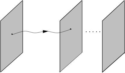
Figure 5: An open string (wavy line) stretching from a single D2-brane (shaded region) to a cluster of $N$ D2-branes carrying $q$ units of D0-brane charge. Quantization of the point particle at the left end of the string produces a Hilbert space ${\cal H}={\cal H}_{1,0}$ while quantization at the right end yields ${\cal H}^{\prime}={\cal H}_{N,q}$.

Canonical quantization is then tantamount to taking $\hat{y}^{i}$ to be multiplication operators by $y^{i}$ and $\hat{s}^{i}$ the canonical momentum operators

$$\hat{s}^{i}=i\,\theta^{ij}\,\frac{\partial}{\partial y^{j}}\ .$$ (6.64)

The physical Hilbert space ${\cal M}$ of open string ground states thus consists of functions on an ordinary torus ${\bf T}^{2}$ with coordinates $y$. The algebras of functions at the left and right endpoints of the open string are thereby generated by operators of the type (6.41) and (6.43), respectively (c.f. (5.6)). In the general case, the map $\Theta\mapsto\Theta^{\prime}$ in (6.21) represents the Morita equivalence between the Heisenberg modules ${\cal H}_{1,0}$ and ${\cal H}_{N,q}$, and it coincides with the $T$-duality transformation that maps a configuration of (D2,D0) brane charges $(1,0)$ to a brane cluster of charges $(N,q)$. The latter collection of D2-branes supports a $U(N)$ Chan-Paton gauge bundle with connection of constant curvature $q/N$. The Hilbert space ${\cal H}_{N,q}$ may then be constructed explicitly by quantizing open strings on an $N^{2}$-fold cover of ${\bf T}^{2}$ that end on a cluster with brane charges $(1,Nq)$, which can be easily described by the modular transformation $B\mapsto B+NQ$ of the action in (6.62) governing the dynamics of $\tilde{x}\in{\bf T}^{2}$, and then orbifolding by the action of the discrete group ${\hbox{\mybb Z}}_{N}\times{\hbox{\mybb Z}}_{N}$ [35]. Generally, the different algebras obtained by quantizing open strings with different boundary conditions, in the low-energy limit with fixed open string parameters, are all Morita equivalent [35]. The equivalence bi-modules are generated by the open string tachyon states with a given boundary condition on the left and another one on the right. That the actions of a pair of algebras commute with each other in these modules follows from the fact that they act at opposite ends of the open strings. That they act irreducibly on the bi-modules follows from the fact that they generate the full algebra of observables in the quantum mechanics of the open string ground states, a point we shall return to in section 8. It is for this latter reason in fact that the modules above are refered to as Heisenberg modules.

7 Matrix Models of Noncommutative Yang-Mills Theory

As we discussed in section 1, noncommutative gauge theories in string theory originally appeared through the large $N$ limits of matrix models. There is in fact a very deep relationship between matrix models and noncommutative Yang-Mills theory that we shall now spend some time analysing. This will be particularly useful for our analysis in the next section. Moreover, it demonstrates the existence of a very natural non-perturbative regularization of noncommutative gauge theories which has no counterpart in ordinary quantum field theory. This in itself proves that these models exist as well-defined field theories, even beyond perturbation theory. Henceforth we shall focus our attention on the simplest instance of structure group rank $N=1$. That the ensuing conclusions hold as well without loss of generality for the generic cases will become clearer in section 8.3. For the remainder of this paper, we shall also assume for simplicity that the spacetime dimensionality $D=2d$ is even and that $\theta^{ij}$ is non-degenerate.

7.1 Twisted Reduced Models

The remarkable aspect of noncommutative gauge theory that we shall build on in this section is the fact that the derivatives $\partial_{i}$ (or $\hat{\partial}_{i}$) can be completely absorbed into the noncommutative gauge fields. There is no analog of the following manipulation in ordinary, commutative Yang-Mills theory. For this, we introduce the covariant coordinates [135]

$$C_{i}=\left(\theta^{-1}\right)_{ij}\,x^{j}+A_{i}$$ (7.1)

which, on using the representation (2.21), are seen to transform covariantly under the noncommutative gauge transformations (4.10),

$$C_{i}~{}\longmapsto~{}g\star C_{i}\star g^{\dagger}\ .$$ (7.2)

In this sense, the operators (7.1) may be thought of as the gauge covariant momentum operators that one introduces in the quantum mechanics of a charged particle in a background magnetic field (c.f. section 1.3). Indeed, they are completely analogous to the covariant derivative operators (5.37) introduced in the case of a constant background flux. Their remarkable property though in the present context is that the entire noncommutative gauge theory may be expressed in terms of them. The star-gauge covariant derivatives $\nabla_{i}$, defined by (4.28), are given as the star-commutators

$$\nabla_{i}f=i\,f\star C_{i}-i\,C_{i}\star f\ ,$$ (7.3)

while the field strength tensor (4.4) is the sum

$$F_{ij}=-i\,\Bigl{(}C_{i}\star C_{j}-C_{j}\star C_{i}\Bigr{)}+\left(\theta^{-1}\right)_{ij}\ .$$ (7.4)

Notice that the operators (7.1) are essentially elements of the abstract, deformed algebra of functions, and so from (7.4) we see that spacetime derivatives have completely disappeared in this rewriting from the action (4.3).

Passing to the Weyl representation $\hat{C}_{i}={\hat{\cal W}}[C]_{i}$, the noncommutative Yang-Mills action (4.2) may then be written as

$$S_{\rm YM}=-\frac{1}{4g^{2}}\,\>{\rm Tr}\,\,\sum_{i\neq j}\left(-i\,\left[\hat{C}_{i}\,,\,\hat{C}_{j}\right]+\left(\theta^{-1}\right)_{ij}\right)^{2}\ .$$ (7.5)

The classical vacua of the gauge theory, i.e. the flat noncommutative gauge fields with $F_{ij}=0$, are in the representation (7.5) interpreted as the momenta which obey the commutation relations $[\hat{C}_{i},\hat{C}_{j}]=-i\,(\theta^{-1})_{ij}$. The remarkable feature of the action (7.5) is that it is just an infinite dimensional matrix model action, as the fields $\hat{C}_{i}$ are formally space independent, i.e. it is a large $N$ version of the matrix model action (1.5). Such a theory is known as a reduced model, becomes it formally derives from the dimensional reduction of gauge theory by taking all fields to be independent of the spacetime coordinates. In fact, one could start from the action (7.5), expand the infinite matrices $\hat{C}_{i}$ as in (7.1) with a noncommuting background (1.1), and thereby derive noncommutative gauge theory from a large $N$ matrix model. Such a matrix expansion about a non-trivial background is the way that noncommutative Yang-Mills theory is obtained from the large $N$ limit of the IIB matrix model (1.5) [44]. The spacetime dependence appears from expanding around a classical vacuum, but initially it is hidden in the infinitely many degrees of freedom of the large $N$ matrices $\hat{C}_{i}$. This is in fact the basis of the original appearence of noncommutative gauge theory from string theory [29].

This intimate connection with reduced models is just a special instance of the Eguchi-Kawai reduction of multi-colour field theories [136] which was argued long ago to reproduce the physics of ordinary, large $N$ Yang-Mills theory. The addition of the constants $(\theta^{-1})_{ij}$ in (7.5) removes what would otherwise be an infinite constant and corresponds to a “twist” in the reduced model [137]. It is required in order that the reduced model be equivalent to the ’t Hooft limit [68] of large $N$ quantum field theory on continuum spacetime, precisely it restores a certain symmetry of the theory that is otherwise broken in the loop expansion of the model. The fact that noncommutative gauge theories are deeply connected to matrix models implies some rather surprising aspects of them and their gauge groups that we shall now proceed to explore.

7.2 Finite-Dimensional Representations

The twisted reduced model (7.5) is intrinsically infinite-dimensional, because its classical equations of motion admit solutions only over an infinite-dimensional Hilbert space, as is usual for Heisenberg-type commutation relations (see the next section). This simply indicates that we must specify derivatives for it somehow. We can now ask whether there exists a finite dimensional, $N\times N$ matrix model version of (7.5) which reproduces noncommutative Yang-Mills theory in the large $N$ limit, as these are the types of models in string theory from which one starts from. Of course, any operator representation of noncommutative gauge theory is formally a matrix model, but we are really seeking a finite-dimensional version which can regulate the continuum quantum field theory at a non-perturbative level. Such a matrix model does indeed exist [96, 97]. Detailed reviews of these constructions are given in [138]. Related work can also be found in [139].

7.2.1 The Twisted Eguchi-Kawai Model

A regulated, $N\times N$ matrix model formulation of noncommutative gauge theory is provided by the twisted Eguchi-Kawai model [137]. The action is

$$S_{\rm TEK}=-\frac{1}{4g^{2}}\,\sum_{i\neq j}\zeta_{ij}^{*}\,\>{\rm tr}\,^{~{}}_{N}\left(V_{i}\,V_{j}\,V_{i}^{\dagger}\,V_{j}^{\dagger}\right)\ ,$$ (7.6)

where $V_{i}$, $i=1,\dots,D$, are $N\times N$ unitary matrices and the ${\hbox{\mybb Z}}_{N}$-valued twist factors are given by

$$\zeta_{ij}={\,\rm e}\,^{2\pi iQ_{ij}/N}\ ,$$ (7.7)

with $Q$ an antisymmetric $D\times D$ integral matrix. This action is the natural non-perturbative analog of the infinite-dimensional matrix model (7.5). By identifying $V_{i}={\,\rm e}\,^{i\epsilon\hat{C}_{i}}$, with $\epsilon$ a dimensionful lattice spacing, the action (7.5) is obtained in the continuum limit of the twisted Eguchi-Kawai model corresponding to $\epsilon\to 0$, $N\to\infty$, and

$$\left(\theta^{-1}\right)_{ij}=\frac{2\pi Q_{ij}}{N\epsilon^{2}}\ .$$ (7.8)

Identifications of this sort are of course well-known. It is the basis of Weyl’s finite version of quantum mechanics [54] which follows from the simple observation that while the Heisenberg commutation relations do not admit any finite dimensional representations, their exponentiated form in terms of unitary operators do in some special instances.

The unitary matrix model (7.6) originates from the ordinary, Wilson lattice gauge theory version [140] of the commutative counterpart of the torus model with background ’t Hooft flux that we studied in section 5.3. The commutative action is given by

$$S_{\rm W}=-\frac{1}{4g^{2}}\,\sum_{x}\,\sum_{i\neq j}\>{\rm tr}\,^{~{}}_{N}\left[U_{i}(x)\,U_{j}(x+\epsilon\,\hat{\imath})\,U_{i}(x+\epsilon\,\hat{\jmath})^{\dagger}\,U_{j}(x)^{\dagger}\right]\ ,$$ (7.9)

where the sum over $x$ runs through sites on a periodic hypercubic lattice, and the gauge fields $U_{i}(x)$ are $N\times N$ unitary matrices on the links of the lattice. As in section 5.3, we assume that the gauge fields are multi-valued functions around the periods of the lattice. They thereby satisfy exponentiated, discrete versions of the twisted boundary conditions (5.20). However, we recall from the discussion at the end of section 5.3 that in the commutative case we may choose $\alpha=0$ in the transition functions (5.22), so that the $\Omega_{i}$ are constant and given by the twist eating solutions $\Gamma_{i}$. Now let us dimensionally reduce the action (7.9) to the point $x=0$. Then, up to an irrelevant dimensionless volume factor, the reduced model describes a one-plaquette version of lattice gauge theory with multi-valued gauge fields. We can use this multi-valuedness to generate the gauge fields at the other corners of the plaquette from the unitary matrix $U_{i}\equiv U_{i}(0)$ via the twisted boundary conditions

$$U_{i}(\epsilon\,\hat{\jmath})=\Gamma_{j}\,U_{i}\,\Gamma_{j}^{\dagger}\ .$$ (7.10)

Substituting (7.10) into the reduced action induced from (7.9) yields

$$S_{\rm W}^{\rm red}=-\frac{1}{4g^{2}}\,\sum_{i\neq j}\>{\rm tr}\,_{N}^{~{}}\left(U_{i}\,\Gamma_{i}\,U_{j}\,\Gamma_{i}^{\dagger}\,\Gamma_{j}\,U_{i}^{\dagger}\,\Gamma_{j}^{\dagger}\,U_{j}^{\dagger}\right)\ .$$ (7.11)

By using the Weyl-’t Hooft commutation relations (5.23) and defining the unitary matrices

$$V_{i}=U_{i}\,\Gamma_{i}\ ,$$ (7.12)

the action (7.11) reduces to (7.6).

As we mentioned in the previous subsection, the twisted Eguchi-Kawai model was originally used as a matrix model which is equivalent to Yang-Mills gauge theory in the large $N$ limit. However, for finite $N$ the model admits another interpretation, which leads to a complete justification of the result that noncommutative gauge theory is equivalent to all orders of perturbation theory to a twisted large $N$ reduced model, namely the IIB matrix model (1.5) with D-brane backgrounds [44]. For this, we will assume, for simplicity, that the rank $N$ of the unitary matrices is an odd integer. Note that the action (7.6) possesses the global $U(N)$ gauge symmetry

$$V_{i}~{}\longmapsto~{}\Omega\,V_{i}\,\Omega^{\dagger}~{}~{}~{}~{}~{}~{},~{}~{}~{}~{}~{}~{}\Omega\in U(N)\ ,$$ (7.13)

and a $U(1)^{D}$ center symmetry

$$V_{i}~{}\longmapsto~{}{\,\rm e}\,^{i\alpha_{i}}\,V_{i}~{}~{}~{}~{}~{}~{},~{}~{}~{}~{}~{}~{}\alpha_{i}\in{\hbox{\mybb R}}\ .$$ (7.14)

The vacuum configuration $V_{i}^{(0)}$ of the theory is given, up to a $U(N)$ gauge transformation (7.13), by the twist-eating solutions for $SU(N)$,

$$V_{i}^{(0)}=\Gamma_{i}\ .$$ (7.15)

We will also restrict the twist matrices and rank to be of the form

$$Q_{ij}=2L^{d-1}\,\varepsilon_{ij}~{}~{}~{}~{}~{}~{},~{}~{}~{}~{}~{}~{}N=L^{d}\ ,$$ (7.16)

where $L$ is an odd integer and $\varepsilon$ is the $D\times D$ skew-diagonal matrix defined by

$$\varepsilon=\pmatrix{0&-1\cr 1&0\cr}\otimes{1\!\!1}_{d}\ .$$ (7.17)

Then, following the general construction of section 6.1, we have $N_{\alpha}=L$, $q_{\alpha}^{\prime}=1$ for each $\alpha=1,\dots,d$, and $N_{0}=1$. It follows that the $SU(N)$ twist eaters are all constructed from $L\times L$ clock and shift matrices. They therefore satisfy $(\Gamma_{i})^{L}={1\!\!1}_{N}$. Note that the constraint (6.8) may then be satisfied by taking $a_{\alpha}=0$, $b_{\alpha}=1$ for each $\alpha=1,\dots,d$ without loss of generality.

7.2.2 The Matrix-Field Correspondence

The relationship between the unitary matrix model (7.6) and noncommutative gauge theory comes about because there is a very natural finite-dimensional version of the Weyl-Wigner correspondence. Let us introduce the $N\times N$ unitary, unimodular matrices

$$J_{k}=\prod_{i=1}^{D}\,(\Gamma_{i})^{k_{i}}\,\prod_{j<i}{\,\rm e}\,^{\pi iQ_{ij}k_{i}k_{j}/N}$$ (7.18)

defined for integer-valued vectors $k$. The phase factor is included in (7.18) to symmetrically order the product of twist eaters. Since $(\Gamma_{i})^{L}={1\!\!1}_{N}$, these matrices have the periodicity properties

$$J_{L-k}=J_{-k}=J_{k}^{\dagger}\ ,$$ (7.19)

and they obey the algebraic relations

$$J_{k}\,J_{q}=\prod_{i=1}^{D}\,\prod_{j=1}^{D}{\,\rm e}\,^{\pi ik_{i}Q_{ij}q_{j}/N}~{}J_{k+q}\ .$$ (7.20)

The $J_{k}$’s have the same formal algebraic properties as the plane wave Weyl basis ${\,\rm e}\,^{ik_{i}\hat{x}^{i}}$ for the continuum noncommutative field theory on the torus. The basic operators were defined in (5.3) and are the analogs of the twist eaters $\Gamma_{i}$ in the present case. Owing to the property (7.19), there are only $N^{2}$ independent matrices. As we will see, the integers $k_{i}$ label momenta on a periodic lattice which are restricted to a Brillouin zone $k\in{\hbox{\mybb Z}}_{L}^{D}$.

The matrices (7.18) obey the orthonormality and completeness relations

$$\frac{1}{N}\,\>{\rm tr}\,^{~{}}_{N}\left(J_{k}\,J_{q}^{\dagger}\right) = \delta_{k,q\,({\rm mod}\,L)}\ ,$$

$$\frac{1}{N}\,\sum_{k\in{\hbox{\mybbs Z}}_{L}^{D}}\,\left(J_{k}\right)_{\mu\nu}\,\left(J_{k}\right)_{\lambda\rho} = \delta_{\mu\rho}\,\delta_{\nu\lambda}\ .$$ (7.21)

They thereby form the Weyl basis for the linear space $gl(N,{\hbox{\mybb C}})$ of $N\times N$ complex matrices [54, 141]. In particular, the fluctuation modes $U_{i}$ in (7.12) about the classical vacuum configuration (7.15) can be expanded as

$$U_{i}=\frac{1}{N^{2}}\,\sum_{k\in{\hbox{\mybbs Z}}_{L}^{D}}U_{i}(k)~{}J_{k}~{}~{}~{}~{}~{}~{},~{}~{}~{}~{}~{}~{}U_{i}(k)=N\,\>{\rm tr}\,^{~{}}_{N}\left(U_{i}\,J_{k}^{\dagger}\right)\ ,$$ (7.22)

where the c-numbers $U_{i}(k)$ may be interpreted as Fourier coefficients for the expansion of a lattice field on the discrete torus. These $N^{2}$ momentum space coefficients now describe the dynamical degrees of freedom in the twisted Eguchi-Kawai model. The underlying discrete, noncommutative space described by these matrices is sometimes called a fuzzy torus.

We can now make a discrete Fourier transformation to define lattice fields on a discrete torus. In complete analogy with the continuum formalism, we define these via the $N\times N$ matrix fields

$$\Delta(x)=\frac{1}{N^{2}}\,\sum_{k\in{\hbox{\mybbs Z}}_{L}^{D}}J_{k}~{}{\,\rm e}\,^{-2\pi ik_{i}x^{i}/\ell}\ ,$$ (7.23)

where

$$\ell=\epsilon\,L$$ (7.24)

is the dimensionful extent of the hypercubic lattice with $N^{2}=L^{D}$ sites $x^{i}$. Because of the relations (7.19), the matrices $\Delta(x)$ are Hermitian and periodic in $x^{i}$ with period $\ell$. This means that the underlying lattice is a discrete torus. Since the algebraic relations satisfied by the matrices $J_{k}$ are completely analogous to their continuum counterparts, the matrices (7.23) have the same formal properties as the continuum ones (5.8) and thereby yield an invertible map between $N\times N$ matrices and lattice fields. In particular, they obey the relations

$$\>{\rm tr}\,^{~{}}_{N}\Bigl{(}J_{k}\,\Delta(x)\Bigr{)} = \frac{1}{N}~{}{\,\rm e}\,^{2\pi ik_{i}x^{i}/\ell}\ ,$$

$$\frac{1}{N}\,\sum_{x}\,\Delta(x)_{\mu\nu}\,\Delta(x)_{\lambda\rho} = \delta_{\mu\rho}\,\delta_{\nu\lambda}\ ,$$

$$\frac{1}{N}\,\>{\rm tr}\,^{~{}}_{N}\Bigl{(}\Delta(x)\,\Delta(y)\Bigr{)} = N^{2}\,\delta_{x,y\,({\rm mod}\,\ell)}\ .$$ (7.25)

A lattice field may then be associated to the unitary matrix $U_{i}$ by the Fourier series

$${\cal U}_{i}(x)\equiv\frac{1}{N^{2}}\,\sum_{k\in{\hbox{\mybbs Z}}_{L}^{D}}U_{i}(k)~{}{\,\rm e}\,^{2\pi ik_{i}x^{i}/\ell}=\frac{1}{N}\,\>{\rm tr}\,^{~{}}_{N}\Bigl{(}U_{i}\,\Delta(x)\Bigr{)}\ .$$ (7.26)

Because of the relation (7.16), the field ${\cal U}_{i}(x)$, which depends on $L^{D}$ spacetime points, describes the same $N^{2}$ degrees of freedom as the $N\times N$ unitary matrix $U_{i}$. In fact, as we will see below, the matrix trace $\>{\rm tr}\,^{~{}}_{N}$ can be substituted by a summation $\sum_{x}$ over lattice points, in complete analogy again with the continuum property (2.11). However, while the matrices $J_{k}$ are unitary as in (7.19), their linear combination in (7.22) need not be unitary in general (a linear combination of unitary matrices does not necessarily stay in the group $U(N)$). Instead, the unitarity condition $U_{i}\,U_{i}^{\dagger}=U_{i}^{\dagger}\,U_{i}={1\!\!1}_{N}$ on the matrices

$$U_{i}=\frac{1}{N^{2}}\,\sum_{x}\,{\cal U}_{i}(x)\,\Delta(x)$$ (7.27)

reads

$${\cal U}_{i}(x)\star{\cal U}_{i}(x)^{*}={\cal U}_{i}(x)^{*}\star{\cal U}_{i}(x)=1\ ,$$ (7.28)

where the lattice star-product is defined by

$${\cal F}(x)\star{\cal G}(x) \equiv \frac{1}{N}\,\>{\rm tr}\,^{~{}}_{N}\Bigl{(}F\,G\,\Delta(x)\Bigr{)}$$ (7.29)

$$= \frac{1}{N^{2}}\,\sum_{y}\,\sum_{z}{\cal F}(x+y)\,{\cal G}(x+z)~{}{\,\rm e}\,^{2i(\theta^{-1})_{ij}y^{i}z^{j}}$$

with (dimensionful) noncommutativity parameter

$$\theta_{ij}=\frac{\epsilon^{2}L}{\pi}\,\varepsilon_{ij}\ .$$ (7.30)

The star-product (7.29) reduces to the Fourier integral kernel representation (2.17) in the continuum limit $\epsilon\to 0$. It is a proper discretized, finite-dimensional form of the continuum Groenewold-Moyal star-product, with which it shares the same algebraic properties (with spacetime integrals replaced by lattice sums).

7.2.3 Discrete Noncommutative Yang-Mills Theory

We are finally ready to interpret the twisted Eguchi-Kawai model in terms of noncommutative gauge theory. For this, we substitute (7.12) and the completeness relation

$$\frac{1}{N^{2}}\,\sum_{x}\,\Delta(x)={1\!\!1}_{N}$$ (7.31)

into the action (7.6) to write

$$S_{\rm TEK}=-\frac{1}{4g^{2}N^{2}}\,\sum_{x}\,\sum_{i\neq j}\>{\rm tr}\,_{N}^{~{}}\left[U_{i}\,\Bigl{(}\Gamma_{i}\,U_{j}\,\Gamma_{i}^{\dagger}\Bigr{)}\,\Bigl{(}\Gamma_{j}\,U_{i}^{\dagger}\,\Gamma_{j}^{\dagger}\Bigr{)}\,U_{j}^{\dagger}\,\Delta(x)\right]\ ,$$ (7.32)

where we have used the Weyl-’t Hooft algebra (5.23) to rearrange the twist eaters in (7.32). The key observation now is that the matrices $\Gamma_{i}$ act as lattice shift operators in this picture, i.e. they are discrete derivatives ${\,\rm e}\,^{\epsilon\hat{\partial}_{i}}$. Using (7.18), (7.23) and (5.23) we may easily compute

$$\Gamma_{i}\,\Delta(x)\,\Gamma_{i}^{\dagger}=\Delta(x-\epsilon\,\hat{\imath})\ ,$$ (7.33)

from which it follows that shifts of the lattice gauge fields may be represented as

$${\cal U}_{i}(x+\epsilon\,\hat{\jmath})=\frac{1}{N}\,\>{\rm tr}\,^{~{}}_{N}\Bigl{(}\Gamma_{j}\,U_{i}\,\Gamma_{j}^{\dagger}\,\Delta(x)\Bigr{)}\ .$$ (7.34)

Using (7.26), (7.29) and (7.34), the action (7.32) finally becomes

$$S_{\rm TEK}=-\frac{1}{4\lambda^{2}}\,\sum_{x}\,\sum_{i\neq j}\,{\cal U}_{i}(x)\star{\cal U}_{j}(x+\epsilon\,\hat{\imath})\star{\cal U}_{i}(x+\epsilon\,\hat{\jmath})^{*}\star{\cal U}_{j}(x)^{*}\ ,$$ (7.35)

where

$$\lambda=\sqrt{g^{2}N}$$ (7.36)

is the ’t Hooft coupling constant.

Thus the twisted Eguchi-Kawai model (7.6) can be rewritten exactly as the noncommutative $U(1)$ lattice gauge theory (7.35). Using the matrix-field correspondence established above, we see that the $U(N)$ invariance (7.13) of the unitary matrix model translates into the local star-gauge symmetry of the lattice model,

$${\cal U}_{i}(x)~{}\longmapsto~{}g(x)\star{\cal U}_{i}(x)\star g(x+\epsilon\,\hat{\imath})^{*}\ ,$$ (7.37)

where $g(x)$ is a star-unitary lattice field, $g(x)\star g(x)^{*}=g(x)^{*}\star g(x)=1$. The lattice gauge theory (7.35) reduces to the Wilson plaquette model (7.9) in the commutative limit $\theta\to 0$. It is in this sense that the twisted Eguchi-Kawai model can be interpreted as noncommutative $U(1)$ Yang-Mills theory (on a periodic lattice). In particular, the matrix model provides a non-perturbative regularization of the field theory, and all results derived in this setting will be completely rigorous. For example, the integration measure for the path integral of the twisted Eguchi-Kawai model is determined in terms of the invariant Haar measures $[dU_{i}]$ for the unitary Lie group $U(N)$, which are invariant under the gauge transformations (7.13). Using the above correspondence it determines the Feynman measure for path integration in the noncommutative gauge theory (7.35) which is invariant under the lattice star-gauge transformations (7.37) as

$$\prod_{x}\,\prod_{i=1}^{D}\,\Bigl{[}d\,{\cal U}_{i}(x)\Bigr{]}=\prod_{k\in{\hbox{\mybbs Z}}_{L}^{D}}\,\prod_{i=1}^{D}\,\Bigl{[}dU_{i}(k)\Bigr{]}=\prod_{i=1}^{D}\,[dU_{i}]\ .$$ (7.38)

The simplicity in writing down the quantum theory here, as compared to the continuum case, is a consequence of the mapping of the $N\times N$ matrix degrees of freedom into a lattice of size $N^{2}=L^{D}$ and with $U(1)$ fields. In particular, we can identify the star-gauge symmetry group of the $U(1)$ noncommutative gauge theory (7.35) with the symmetry group $U(L^{d})$ of the unitary matrix model. These facts will all be instrumental in the analysis of the next section.

We will conclude our discussion of the matrix model formulations of noncommutative Yang-Mills theories with a number of remarks concerning the above construction:

• There are two sorts of continuum limits that the lattice gauge theory (7.35) admits. If we take the limit $N=L^{d}\to\infty$ first for finite lattice spacing $\epsilon$, followed by the continuum limit $\epsilon\to 0$, then from (7.30) it follows that $\theta\to\infty$ and hence only planar Feynman diagrams survive (c.f. (3.16)). This is the usual way to reproduce the ’t Hooft limit of ordinary large $N$ Yang-Mills theory on continuum spacetime from twisted reduced models [137]. Alternatively, we can take the continuum limit of the reduced model by keeping the noncommutativity $\theta$ fixed in the correlated limit $N\to\infty$, $\epsilon\to 0$, with $L\epsilon^{2}$ finite. The extent of the lattice (7.24) in this limit is $\ell\sim\sqrt{L}=N^{1/D}\to\infty$, and we recover noncommutative gauge theory on flat, infinite space ${\hbox{\mybb R}}^{D}$, as in the large $N$ limit of the IIB matrix model [44]. In both types of large $N$ limits the Yang-Mills coupling constant $g$ must be tuned to be a function of $\epsilon$, in order that the ’t Hooft coupling constant (7.36) be finite in the limit. The case of finite $N$ corresponds to the noncommutative version (7.35) of Wilson lattice gauge theory, which is a non-perturbative lattice regularization of the continuum noncommutative Yang-Mills theory. We have thereby formulated a well-defined finite-dimensional matrix model representation of noncommutative Yang-Mills theory on ${\hbox{\mybb R}}^{D}$. Among other things, this relationship completes the explanation of the remarkable coincidence of the perturbative beta-functions in the planar commutative and noncommutative gauge theories that we discussed in section 4.3.

• Given that the twisted Eguchi-Kawai model is derived as the dimensional reduction of the Wilson lattice gauge theory (7.9) with background ’t Hooft flux, it would appear that we have also derived a relationship between this latter, commutative lattice gauge theory and the noncommutative lattice gauge theory (7.35) which has single-valued fields. The two theories are in fact Morita equivalent [97]. Noncommutative lattice gauge theory is always Morita equivalent to a commutative lattice gauge theory, because the finite dimensionality of the representation of the noncommutative algebra of functions on the lattice necessitates a rational-valued dimensionless deformation parameter $\Theta$. This establishes that the phenomenon of Morita equivalence of noncommutative gauge theories holds in and beyond regulated perturbation theory.

• It is possible to generalize the construction of this subsection to induce a noncommutative $U(r)$ lattice gauge theory with rank $r>1$. For this, we take the unitary matrices of the twisted Eguchi-Kawai model to live in a direct product group $U(r)\otimes U(N)$. The trace over the $U(N)$ indices is treated as before and transformed into a sum over lattice points. The remaining indices are left unaltered and become the non-abelian colour indices of the resulting field theory. This is tantamount to choosing a more general background flux $Q$ for which $N_{0}>1$, as we did in the derivation of Morita equivalence in section 6.

• The noncommutativity parameter (7.30) can be written as $\theta=\ell\epsilon/\pi$, so that finite noncommutativity requires keeping the quantity $\ell\epsilon$ fixed in the continuum limit. In fact, finite noncommutativity in the lattice formulation necessarily implies a finite size $\ell=\pi\theta/\epsilon$ of the spacetime [97]. As the lattice spacing $\epsilon$ is an ultraviolet cutoff for the dynamics of the field theory and $\ell$ serves as an infrared cutoff, this is just a non-perturbative manifestation of the UV/IR mixing phenomenon in noncommutative quantum field theory that we unravelled in section 3.3. It is very explicitly evident in the discrete formalism that the two limits $\ell\to\infty$ (giving the noncommutative planar limit) and $\epsilon\to 0$ (giving the commutative limit) do not commute. This gives a very direct interpretation of this novel property of noncommutative field theories, which in the present case occurs at a kinematical level. The reason for this is the very drastic regularization provided by the matrix model.

• It is possible to modify the above construction and arrive at a continuum gauge theory on a noncommutative torus. Within the present framework this is not possible, because from (7.24) and (7.30) it follows that it is not possible to take a large $N$ continuum limit which keeps both the size and noncommutativity of the spacetime finite. One can, however, repeat the above construction by introducing two more integers $n$ and $m$ with $L=nm$, and modifying the map (7.23) to [96]

  $$\Delta_{n}(x)=\frac{1}{N^{2}}\,\sum_{k\in{\hbox{\mybbs Z}}_{m}^{D}}\left(J_{k}\right)^{n}~{}{\,\rm e}\,^{-2\pi ik_{i}x^{i}/\epsilon m}\ .$$ (7.39)

  The $N\times N$ matrix-valued lattice fields (7.39) provide a one-to-one Weyl-Wigner correspondence between lattice fields and elements of $gl(N,{\hbox{\mybb C}})$ which commute with the matrices

  $$\Omega_{i}=\prod_{j=1}^{D}\left(\Gamma_{j}\right)^{m\varepsilon_{ij}}\ .$$ (7.40)

  The resulting noncommutative lattice gauge theories thereby follow from the constrained twisted Eguchi-Kawai model (7.6) obtained by restricting its unitary matrices (7.12) to those which obey the constraints $U_{i}\,\Omega_{j}=\Omega_{j}\,U_{i}$ for each $i,j=1,\dots,D$. Since $(\Gamma_{i})^{L}={1\!\!1}_{N}$, for $n=1$ the matrices (7.40) are trivial and we recover the previous construction, with $\Delta(x)=\Delta_{1}(x)$. For $n>1$ the dimensionless noncommutativity parameter is $\Theta=n/m$ and it is possible keep the noncommutativity of spacetime finite as $N\to\infty$ even for finite extent $\epsilon m$. Thus the resulting continuum noncommutative field theory lives on a torus. The geometrical meaning of the constraints is that they enforce the compactification of the matrices of the unitary matrix model on a $d$-dimensional torus [96]. Indeed, they are just equivalent to unitary versions of the quotient conditions [29] for toroidal compactifications of the IIB matrix model (1.5). Unlike this Hermitian matrix model, the quotient conditions for the unitary matrix model admit finite-dimensional solutions. The resulting solutions also have a natural interpretation in terms of Morita equivalences of noncommutative tori [96]. It is also possible to view such correspondences between matrix models and lattice field theories by using only Morita equivalence [97], without the quotient conditions, but with more complicated twist matrices $Q$. Such generalizations also allow the construction of noncommutative field theories with the most general deformation parameters $\theta_{ij}$. We should point out, however, that the noncommutative lattice gauge theories which originate from twisted reduced models are not the only ones that can be constructed [97].

8 Geometry and Topology of Star-Gauge Transformations

In this final section we will take a look at the structure of the group of star-gauge transformations in noncommutative Yang-Mills theory. Gauge symmetries in the noncommutative case are very different from their commutative counterparts, because they involve an intriguing mixing between spacetime and internal, $U(N)$ symmetries. This mixing was responsible for the duality that we described in the previous section, in that the spacetime degrees of freedom were able to absorb some of the colour degrees of freedom of the gauge fields. It is evident in fact immediately from the operatorial form of the noncommutative Yang-Mills action (4.2), which shows how the spacetime and $U(N)$ traces are interlocked and cannot be separated from one another. We recall that for this reason it was difficult to construct local, star-gauge invariant observables. Another aspect of noncommutative gauge theory which is intimately tied to the mixing between spacetime and gauge degrees of freedom was its connection with matrix models, which followed from the observation that all derivatives, and hence all spacetime dependence, can be completely absorbed into the noncommutative gauge fields. This is particularly transparent in the discrete representations of the previous section, whereby the $N\times N$ matrix degrees of freedom are in a one-to-one correspondence with $N^{2}$ spacetime lattice points.

In the remainder of this paper we will pose a very elementary question: What is the gauge symmetry group of noncommutative Yang-Mills theory on flat infinite space? In our attempt to formulate an answer to this question, we will be guided by two main themes, with the aim of clarifying the structure of the local and global star-gauge symmetry group:

• $\underline{\rm Geometry:}$ We have seen in section 4.2 that spacetime translations can be regarded to a certain extent (to be discussed below) as star-gauge transformations. The only other theory with such a property is general relativity. This feature has been used to suggest [142] that general coordinate transformations may be realized as genuine gauge symmetries of noncommutative Yang-Mills theory. In fact, via certain dimensional reduction techniques [143], the translational symmetry can be gauged to induce a field theory which contains as special limits some gauge models of gravitation. The most compelling evidence however has been via the strong-coupling dual supergravity description of maximally supersymmetric noncommutative Yang-Mills theory in four dimensions, in which it is possible to identify the Newtonian gravitational force law [144]. Other indications include the observation that the unitary group of a closed string vertex operator algebra contains generic reparametrizations of the spacetime coordinates [16, 17] (see [145] for an explicit description of this group), the identification of the one-loop long-ranged potential particular to noncommutative Yang-Mills theory with the gravitational interaction in Type IIB superstring theory [44, 146], and the couplings of noncommutative gauge fields to massless closed string modes in flat space [104]. However, we will see in this section that this assertion is incorrect, in that noncommutative gauge transformations can only realize a certain subgroup of the diffeomorphism group of spacetime [99].

• $\underline{\rm Topology:}$ We are also interested in global properties of noncommutative gauge theories, and the global gauge group is an important object for the topological classification of solitons, among other things. The star-gauge group is infinite-dimensional and has been identified previously as both the infinite unitary group $U(\infty)$ and also as the group $U({\cal H})$ of unitary operators on a separable Hilbert space ${\cal H}$. These two groups are very different, and in fact both of these proposals for the star-gauge group are incorrect. The former group can never be identified with a space of functions (but rather only completions of it can), while the latter group is, as we will discuss, contractible and so it doesn’t possess the interesting topological characteristics that its commutative counterpart has which leads to effects like anomalies and topological solitons.

In this section we will clarify some of these misconceptions, and also illustrate some very precise mathematical aspects of the star-gauge symmetry group of noncommutative Yang-Mills theory. This will bring out some more of the deeper operator-algebraic formalism of noncommutative geometry, already unleashed at the end of section 6. Throughout this section we will denote the algebra of Schwartz functions on ${\hbox{\mybb R}}^{D}\to{\hbox{\mybb C}}$ equipped with the star-product (LABEL:starproddef) by ${\cal A}_{\theta}$. Its commutative limit of ordinary functions will be denoted ${\cal A}_{0}=C({\hbox{\mybb R}}^{D})$. The representation of the algebra ${\cal A}_{\theta}$ by operators on a Hilbert space ${\cal H}$ will be denoted ${\cal A}_{\theta}({\cal H})\subset{\rm End}({\cal H})$. The treatment of this section will mostly employ an operator formalism with Heisenberg commutation relations, mostly ignoring the star product structure. However, within the framework of deformation quantization, the structure of star-gauge symmetries is rather well understood through the formalism of deformed vector bundles [147], along the lines of what we described in section 6.3. Along these lines an important structure which arises is a cocycle condition on the gauge transformations, which is treated implicitly in the operator framework. While the following material is somewhat more mathematical than that of previous sections, it introduces some more fundamental techniques and ideas of noncommutative geometry. Most of the material of this section follows closely [99], where more technical details may be found.

8.1 Star-Gauge Symmetries Revisited

We will begin by defining more precisely the notion of gauge symmetry in the noncommuting setting, and will proceed throughout this subsection in a somewhat abstract fashion. In the commutative case, gauge fields arise through covariant derivatives which specify parallel transport along the fibers of a given vector bundle over ${\hbox{\mybb R}}^{D}$. In turn, as we saw in section 6.3, a vector bundle is completely characterized by its (Hilbert) space of sections. The commutative algebra ${\cal A}_{0}$ acts naturally on this space, so that the sections form an ${\cal A}_{0}$-module. Thus the noncommutative analog of a vector bundle over noncommutative ${\hbox{\mybb R}}^{D}$ is an ${\cal A}_{\theta}$-module ${\cal H}$, whose vectors $\psi$ will be interpreted as fundamental matter fields, i.e. fields which transform under the fundamental representation of the gauge symmetry group. These representations will be particularly important for the explicit identification of the star-gauge symmetry group. We then seek a covariant derivative $\nabla_{i}$ such that $\nabla_{i}\psi$ is a matter field in the same representation as $\psi$. This is the algebraic version of the parallel transport condition.

A canonical choice of projective module is the Hilbert space of square-integrable fundamental matter fields,

$${\cal H}_{\rm m}=L^{2}({\hbox{\mybb R}}^{D})\otimes{\hbox{\mybb C}}^{N}\ .$$ (8.1)

From a geometric standpoint and also to analyse properly the gauge symmetries, we need to investigate the reducibility of this representation of the algebra. To this end, let us begin by analysing the commutative case. We may define an action of ${\cal A}_{0}$ on ${\cal H}_{\rm m}$ by

$$\psi\cdot f=f\,\psi$$ (8.2)

with $f\in{\cal A}_{0}$ and $\psi\in{\cal H}_{\rm m}$. The defining condition of a module, $(\psi\cdot g)\cdot f=\psi\cdot(f\,g)$, is a trivial consequence of the commutativity of pointwise multiplication of functions. We can then decompose the space (8.1) into irreducible components with respect to this action,

$${\cal H}_{\rm m}=\int\limits_{x}\!\!\!\!\!\!\!~{}\!\!\ominus~{}\delta_{x}\otimes{\hbox{\mybb C}}^{N}\ ,$$ (8.3)

where $\delta_{x}:{\cal A}_{0}\to{\hbox{\mybb C}}$ is the evaluation functional at $x\in{\hbox{\mybb R}}^{D}$ defined by

$$\delta_{x}(f)=\int d^{D}y~{}\delta^{D}(x-y)\,f(y)\ .$$ (8.4)

By approximating the delta-function by functions of ${\cal A}_{0}$, we may view the functional $\delta_{x}(f)=f(x)$ as a character of the algebra ${\cal A}_{0}$, and also as a one-dimensional unitary irreducible representation of ${\cal A}_{0}$ on ${\cal H}_{\rm m}$ via pointwise multiplication of functions,

$$\delta_{x}(f)\cdot\psi=f(x)\,\psi\ .$$ (8.5)

We see that the points $x\in{\hbox{\mybb R}}^{D}$ are formally “reconstructed” from the unitary irreducible representations (or equivalently the characters) of the commutative algebra ${\cal A}_{0}$. As discussed at the beginning of section 6, this is the geometric basis of the Gel’fand-Naimark theorem and the association of topological spaces to commutative $C^{*}$-algebras.

Let us now consider the noncommutative case. We may define a right action of ${\cal A}_{\theta}$ on ${\cal H}_{\rm m}$ by

$$\psi\cdot f=\psi\star f\ .$$ (8.6)

The requisite condition $(\psi\cdot g)\cdot f=\psi\cdot(g\star f)$ follows from associativity of the star-product. Such fields $\psi$ are, as we will soon see, naturally interpreted as fundamental matter fields. For a left action $f\cdot\psi=f\star\psi$, the $\psi$’s would instead be thought of as anti-fundamental matter fields. Again, this action defines a reducible representation. To see this, let us rotate coordinates to the Darboux basis (3.6), in which the coordinate operators $\hat{x}^{i}$ split into $d$ mutually commuting blocks in each of which the Heisenberg commutation relations

$$\left[\hat{x}^{2\alpha-1}\,,\,\hat{x}^{2\alpha}\right]=i\,\vartheta_{\alpha}{}~{}~{}~{}~{}~{}~{},~{}~{}~{}~{}~{}~{}\alpha=1,\dots,d$$ (8.7)

hold. By the Stone-von Neumann theorem [148], the Lie algebra (8.7) has a unique irreducible representation, the Hilbert space of quantum mechanics, i.e. the Schrödinger representation ${\cal H}_{\rm q}=L^{2}({\hbox{\mybb R}}^{d})$ seen as functions of the coordinates $x^{2\alpha}$, $\alpha=1,\dots,d$. From this fact it is evident that the Hilbert space (8.1) is reducible.

The Schrödinger ${\cal A}_{\theta}$-module ${\cal H}_{\rm q}$ is a separable Hilbert space, i.e. it is countably infinite-dimensional, because it can be expressed in terms of the usual Fock space of creation and annihilation operators. Mathematically, this is the completion to the space of square-summable sequences

$${\cal H}_{\rm q}\cong\ell^{2}({\hbox{\mybb Z}}_{+}^{d})=\overline{\bigoplus_{\vec{n}\in{\hbox{\mybbs Z}}_{+}^{d}}{\hbox{\mybb C}}\,|\vec{n}\,\rangle}\ ,$$ (8.8)

where $|\vec{n}\,\rangle=|n_{1},\dots,n_{d}\rangle$ is a multi-particle state, and the Fock space creation and annihilation operators are defined by

$$\hat{c}_{\alpha}=\frac{1}{\sqrt{2|\vartheta_{\alpha}|}}\,\left(\hat{x}^{1}+i\,{\rm sgn}(\vartheta_{\alpha})\,\hat{x}^{2}\right)~{}~{}~{}~{}~{}~{},~{}~{}~{}~{}~{}~{}\hat{c}_{\alpha}^{\dagger}=\frac{1}{\sqrt{2|\vartheta_{\alpha}|}}\,\left(\hat{x}^{1}-i\,{\rm sgn}(\vartheta_{\alpha})\,\hat{x}^{2}\right)$$ (8.9)

with the non-vanishing commutation relations

$$\left[\hat{c}_{\alpha}\,,\,\hat{c}_{\beta}^{\dagger}\right]=\delta_{\alpha\beta}\ .$$ (8.10)

The vectors $|\vec{n}\,\rangle$ are then the simultaneous orthonormal eigenstates of the $d$ number operators $\hat{n}_{\alpha}=\hat{c}_{\alpha}^{\dagger}\hat{c}_{\alpha}$ with eigenvalue $n_{\alpha}\in{\hbox{\mybb Z}}_{+}$, $\hat{n}_{\alpha}|\vec{n}\,\rangle=n_{\alpha}|\vec{n}\,\rangle$, and the actions of the operators (8.9) on this basis are defined by

$$\hat{c}_{\alpha}|\vec{n}\,\rangle=\sqrt{n_{\alpha}}\,|\vec{n}-1_{\alpha}\rangle{}~{}~{}~{}~{}~{}~{},~{}~{}~{}~{}~{}~{}\hat{c}_{\alpha}^{\dagger}|\vec{n}\,\rangle=\sqrt{n_{\alpha}+1}\,|\vec{n}+1_{\alpha}\rangle\ ,$$ (8.11)

with $1_{\alpha}$ the integer vector whose components are $(1_{\alpha})_{\beta}=\delta_{\alpha\beta}$. The Hilbert space (8.8) is projective as a right ${\cal A}_{\theta}$-module. To see this, we use (8.9) to expand the Weyl operators (2.4) over the Fock space (8.8), and for each fixed integer vector $\vec{n}_{0}\in{\hbox{\mybb Z}}_{+}^{d}$ consider the operator $\hat{p}_{\vec{n}_{0}}=|\vec{n}_{0}\rangle\langle\vec{n}_{0}|$. It is the orthogonal projection onto the one-dimensional subspace of ${\cal H}_{\rm q}$ spanned by the vector $|\vec{n}_{0}\rangle$. In the Weyl representation of the trivial rank-$N$ ${\cal A}_{\theta}$-module ${\cal H}_{\rm m}$, we may write the orthogonal decomposition ${\cal H}_{\rm m}=\hat{p}_{\vec{n}_{0}}{\cal H}_{\rm m}\oplus({1\!\!1}_{{\cal H}_{\rm q}}-\hat{p}_{\vec{n}_{0}}){\cal H}_{\rm m}$. Under the correspondence $\langle\vec{n}|\leftrightarrow|\vec{n}_{0}\rangle\langle\vec{n}|$, we have the natural isomorphism $\hat{p}_{\vec{n}_{0}}{\cal H}_{\rm m}\cong{\cal H}_{\rm q}$ as right ${\cal A}_{\theta}$-modules, and hence ${\cal H}_{\rm q}$ is projective.

By the stronger Mackey form of the Stone-von Neumann theorem [148] it follows that any ${\cal A}_{\theta}$-module ${\cal H}$ is a direct sum of Fock modules. In particular, by iterating the preceding arguments it follows that the Hilbert space (8.1) contains infinitely many copies of the Schrödinger representation, so that as ${\cal A}_{\theta}$-modules there is a natural isomorphism

$${\cal H}_{\rm m}=\bigoplus_{n=0}^{\infty}{\cal H}_{\rm q}\otimes{\hbox{\mybb C}}^{N}\ .$$ (8.12)

In this sense, Fock space ${\cal H}_{\rm q}$ is the analog of a single point in the noncommutative space. It also follows that any fundamental matter field may be expanded with respect to this decomposition as

$${\hat{\cal W}}[\psi]=\sum_{\vec{n}\in{\hbox{\mybbs Z}}_{+}^{d}}\,\left(\sum_{\vec{m}\in{\hbox{\mybbs Z}}_{+}^{d}}\psi_{\vec{n},\vec{m}}\,|\vec{m}\rangle\right)\langle\vec{n}\,|\ ,$$ (8.13)

where $\psi_{\vec{n},\vec{m}}\in{\hbox{\mybb C}}^{N}$ and the states $\langle\vec{n}\,|$ label the points (Fock representations) on the noncommutative space. Note that the superposition $\sum_{\vec{m}}\psi_{\vec{n},\vec{m}}\,|\vec{m}\rangle$ is an element of ${\cal H}_{\rm q}$ and so is the analog of a field with support at only one point in spacetime. The field (8.13) is in fact an element of the Weyl representation of the algebra ${\cal A}_{\theta}$ on the Hilbert space (8.8), defined by $\psi\cdot f={\hat{\cal W}}[\psi]\,{\hat{\cal W}}[f]$. This simply means that we are working in the defining (or fundamental) representation of ${\cal A}_{\theta}$ and it is completely analogous to the commutative case (8.3,8.4). This superposition carries information about the infinite dimensional unitary gauge symmetry represented on the module ${\cal H}_{\rm q}$. Notice also that the irreducibility of the Fock module automatically implies that all of the algebras ${\cal A}_{\theta}$ for different deformation parameters $\theta$ are Morita equivalent. This is in marked contrast to the noncommutative torus, which possesses a non-trivial topological structure.

In analogy to the commutative case, we may then consider the gauge transformations

$$\psi(x)~{}\longmapsto~{}g(x)\star\psi(x)\ .$$ (8.14)

It commutes with the right action of ${\cal A}_{\theta}$ on ${\cal H}_{\rm m}$ and thereby preserves the representation of the algebra. It also preserves the $L^{2}$-norm of the matter field $\psi$ provided that the gauge function $g(x)$ satisfies the star-unitarity condition (4.8). This implies that $g$ is an element of the group $U(N,{\cal A}_{\theta})=U({\hbox{\mybb M}}(N,{\cal A}_{\theta}))$ of unitary elements of the algebra ${\hbox{\mybb M}}(N,{\cal A}_{\theta})={\cal A}_{\theta}\otimes{\hbox{\mybb M}}(N,{\hbox{\mybb C}})$ of $N\times N$ matrices with entries in the algebra ${\cal A}_{\theta}$. Strictly speaking, however, the algebra ${\cal A}_{\theta}$ of Schwartz functions has no unit and so it is necessary to define unitary elements of the algebra ${\cal A}_{\theta}\oplus{\hbox{\mybb C}}$ obtained from ${\cal A}_{\theta}$ by adjoining an identity element. Geometrically, this extension corresponds to studying functions on the topological (but not metric) one-point compactification of ${\hbox{\mybb R}}^{D}$. While geometrically such a compactification can have dramatic effects on the topological properties of the field theory, it is perfectly harmless at the algebraic level. We shall always implicitly assume such a unital extension, and discuss some of its properties further in section 8.4. The group $U(N,{\cal A}_{\theta})$ is the gauge symmetry group that we shall study in this section.

We now introduce a covariant derivative as the anti-Hermitian operator $\nabla_{i}:{\cal H}_{\rm m}\to{\cal H}_{\rm m}$ defined by

$$\nabla_{i}(\psi)=\partial_{i}\psi-i\,A_{i}\star\psi\ ,$$ (8.15)

where $A_{i}$ is a Hermitian element of the algebra ${\hbox{\mybb M}}(N,{\cal A}_{\theta})$, i.e. a gauge field. This operator has the properties we need. Since the derivative $\partial_{i}$ satisfies the Leibnitz rule with respect to the star-product,

$$\partial_{i}(f\star g)=(\partial_{i}f)\star g+f\star(\partial_{i}g)\ ,$$ (8.16)

it follows that $\nabla_{i}$ satisfies a right Leibnitz rule,

$$\nabla_{i}(\psi\star f)=\psi\star(\partial_{i}f)+\nabla_{i}(\psi)\star f\ .$$ (8.17)

This ensures that $\nabla_{i}(\psi)$ lies in the same representation of the algebra ${\cal A}_{\theta}$ as the matter field $\psi$, as desired. In particular, $\nabla_{i}(\psi)$ should transform in the same way as $\psi$ under the gauge transformations (8.14), which fixes the gauge transformation rule $\nabla_{i}\mapsto\nabla_{i}^{g}$, where

$$\nabla_{i}^{g}(\psi)=g\star\nabla_{i}\left(g^{\dagger}\star\psi\right)\ .$$ (8.18)

By using (8.15) we then find that the covariant transformation law (8.18) is equivalent to the usual star-gauge transformation law (4.10), and also that the noncommutative field strength tensor (4.4) is given by the star-commutator

$$F_{ij}=i\,\nabla_{i}\star\nabla_{j}-i\,\nabla_{j}\star\nabla_{i}\ .$$ (8.19)

It follows that the curvature tensor $F_{ij}\in{\hbox{\mybb M}}(N,{\cal A}_{\theta})$ commutes with the action of ${\cal A}_{\theta}$ on the Hilbert space ${\cal H}_{\rm m}$, and so it lies in the corresponding commutant of the algebra representation, i.e. $F_{ij}\in{\rm End}_{{\cal A}_{\theta}}({\cal H}_{\rm m})$.

The derivation presented in this subsection thereby brings us back to the models of noncommutative Yang-Mills theory that were described in section 4. In particular, the Weyl representation (4.2) gives a rewriting of noncommutative gauge theory as ordinary Yang-Mills theory (on a noncommutative space) with local fields and with the extended, infinite dimensional gauge symmetry group $U(N,{\cal A}_{\theta})$. This point of view has proven fruitful for analysing the renormalization properties of noncommutative Yang-Mills theory [109], and it shows rather explicitly the transmutation of $U(N)$ colour degrees of freedom into spacetime degrees of freedom along the noncommutative directions. We remark also that the fundamental matter fields $\psi(x)$ induce local star-gauge invariant observables of noncommutative gauge theory through the density operators $\rho(x)=\psi(x)^{\dagger}\star\psi(x)$.

8.2 Inner Automorphisms

The discussion of the previous subsection emphasizes, among other things, the point that gauge transformations correspond to the inner automorphisms $f\mapsto g\star f\star g^{\dagger}$ of the algebra ${\hbox{\mybb M}}(N,{\cal A}_{\theta})$. These transformations form the group

$${\rm Inn}(N,{\cal A}_{\theta})=\Bigl{\{}\,\imath_{g}~{}\Bigm{|}~{}\imath_{g}(f)=g\star f\star g^{\dagger}~{},~{}f\in{\hbox{\mybb M}}(N,{\cal A}_{\theta})~{},~{}g\in U(N,{\cal A}_{\theta})\Bigr{\}}\ .$$ (8.20)

They rotate the algebra elements and correspond to internal fluctuations of the spacetime geometry in a sense that we will now describe. In general, the group (8.20) is a proper, normal subgroup of the automorphism group ${\rm Aut}(N,{\cal A}_{\theta})$, the group of transformations which preserve the algebra ${\hbox{\mybb M}}(N,{\cal A}_{\theta})$. The remaining automorphisms are called outer automorphisms and together they form an exact sequence of groups,

$${1\!\!1}^{~{}}_{{\hbox{\mybbs M}}(N,{\cal A}_{\theta})}~{}\longrightarrow~{}{\rm Inn}(N,{\cal A}_{\theta})~{}\longrightarrow~{}{\rm Aut}(N,{\cal A}_{\theta})~{}\longrightarrow~{}{\rm Out}(N,{\cal A}_{\theta})~{}\longrightarrow~{}{1\!\!1}^{~{}}_{{\hbox{\mybbs M}}(N,{\cal A}_{\theta})}\ .$$ (8.21)

Equivalently, the group ${\rm Aut}(N,{\cal A}_{\theta})$ is the semi-direct product of ${\rm Inn}(N,{\cal A}_{\theta})$ by the natural action of ${\rm Out}(N,{\cal A}_{\theta})$ on the elements $\imath_{g}\in{\rm Inn}(N,{\cal A}_{\theta})$.

To get some feel for this somewhat abstract characterization, let us again turn to the commutative limit ${\cal A}_{0}$. Then ${\rm Inn}(N,{\cal A}_{0})$ is the group of $U(N)$ gauge transformations on ${\hbox{\mybb R}}^{D}\to U(N)$, while ${\rm Out}(N,{\cal A}_{0})$ is naturally isomorphic to the group ${\rm Diff}({\hbox{\mybb R}}^{D})$ of diffeomorphisms of ${\hbox{\mybb R}}^{D}$ [149]. Given a smooth function $\phi:{\hbox{\mybb R}}^{D}\to{\hbox{\mybb R}}^{D}$, there is a natural automorphism $\alpha_{\phi}:{\cal A}_{0}\to{\cal A}_{0}$ defined by

$$\alpha_{\phi}(f)=f\circ\phi^{-1}~{}~{}~{}~{}~{}~{},~{}~{}~{}~{}~{}~{}f\in{\cal A}_{0}\ .$$ (8.22)

If we now represent, as in the previous subsection, the algebra ${\cal A}_{0}$ on the Hilbert space ${\cal H}_{\rm m}$ of fundamental matter fields, then evidently all inner automorphisms are given via conjugation by unitary operators on ${\cal H}_{\rm m}$. The same property is in fact true of the outer automorphisms. Given $\phi\in{\rm Diff}({\hbox{\mybb R}}^{D})$, we may define a unitary operator $\hat{g}_{\phi}$ on ${\cal H}_{\rm m}$ by

$$\hat{g}_{\phi}\,\psi(x)=\left|\frac{\partial\phi}{\partial x}\right|^{1/2}\,\psi\left(\phi^{-1}x\right)\ .$$ (8.23)

Thus, in the commutative case the group ${\rm Aut}(N,{\cal A}_{0})$ may be modelled on the group $U({\cal H}_{\rm m})$ of unitary endomorphisms of the Hilbert space (8.1), and the unitary group of ${\cal A}_{0}$ coincides with the ordinary $N\times N$ unitary group $U(N)$ of Yang-Mills theory.

In the noncommutative case $\theta\neq 0$, we will soon see that it is also true that the automorphism group ${\rm Aut}(N,{\cal A}_{\theta})$ is related to the group $U({\cal H})$ of unitary operators on some Hilbert space ${\cal H}$. However, $U({\cal H})$ is not the right candidate for the gauge symmetry group of noncommutative Yang-Mills theory. The problem is that for any separable Hilbert space ${\cal H}$ (one with a countably infinite basis), it is a fundamental fact, known as Kuiper’s theorem [150], that $U({\cal H})$ is contractible, i.e. as a manifold, all closed loops on $U({\cal H})$ can be continuously contracted to a point. In particular, all of its homotopy groups are trivial,

$$\pi_{n}\Bigl{(}U({\cal H})\Bigr{)}=0\ ,$$ (8.24)

and we would thereby lose all of the nice topology residing in noncommutative gauge theory and the ensuing topological configurations like solitons, instantons and D-branes, to name but a few. Furthermore, many such topological quantities should be stable under algebra deformations, i.e. they should be preserved in the commutative limit. The lesson to be learned here is that not all automorphisms of the algebra (or unitary endomorphisms of a Hilbert space) generate gauge transformations, but rather only the inner automorphisms do. We shall soon see what the appropriate gauge group is. For the remainder of this subsection we will describe some more basic aspects of the group of (inner) automorphisms of the noncommutative algebra ${\cal A}_{\theta}$.

8.2.1 The Tomita Involution

A lot of what we have described in this section thus far has been based on the representation of ${\cal A}_{\theta}$ on some Hilbert space ${\cal H}$, and indeed this will be important for the remainder of our discussion. The automorphism group ${\rm Aut}(N,{\cal A}_{\theta})$ may then be computed via its lift to this Hilbert space as [99, 149]

$${\rm Aut}_{\cal H}(N,{\cal A}_{\theta})=\left\{\,\hat{g}\in U({\cal H})~{}\left|~{}\hat{g}\,J=J\,\hat{g}~{},~{}\imath_{\hat{g}}\in{\rm Aut}\Bigl{(}N\,,\,{\cal A}_{\theta}({\cal H})\Bigr{)}\right.\right\}\ .$$ (8.25)

The operator $J$ is called the Tomita involution and it induces a bi-module structure for the given representation of the algebra ${\cal A}_{\theta}$. It is inserted in the definition (8.25) because the structure of the automorphism group of ${\cal A}_{\theta}$ shouldn’t depend on whether the algebra acts on ${\cal H}$ from the right or left. The operator $J$ is formally the anti-linear, self-adjoint unitary isometry of ${\cal H}$ such that $J{\cal A}_{\theta}({\cal H})J^{-1}={\cal A}_{\theta}^{\prime}({\cal H})$ is the commutant of the algebra ${\cal A}_{\theta}$ in the module ${\cal H}$. If ${\cal A}_{\theta}$ acts on ${\cal H}$ from the right (resp. left), then $J{\cal H}$ is a left (resp. right) ${\cal A}_{\theta}$-module. From the Hilbert space lift (8.25) we recover the automorphisms of ${\cal A}_{\theta}$ from the Wigner projection $\Pi:{\rm Aut}_{\cal H}(N,{\cal A}_{\theta})\to{\rm Aut}(N,{\cal A}_{\theta})$ defined by

$$\Pi(\hat{g})\Bigl{[}f(x)\Bigr{]}=\>{\rm Tr}\,^{~{}}_{\cal H}\Bigl{(}\hat{g}\,{\hat{\cal W}}[f]\,\hat{g}^{-1}\,\hat{\Delta}(x)\Bigr{)}\ ,$$ (8.26)

where $\hat{\Delta}(x)$ is the map (2.6) in the representation of ${\cal A}_{\theta}$ on ${\cal H}$, and $\>{\rm Tr}\,^{~{}}_{\cal H}$ denotes the trace over states of the Hilbert space ${\cal H}$. Clearly these constructions also hold true in the restriction of the automorphism group of the algebra to gauge transformations.

A physical interpretation of the Tomita involution $J$ may be given as follows. When ${\cal H}={\cal H}_{\rm m}$ is the Hilbert space (8.1), we define the action of $J$ on fundamental matter fields $\psi$ by

$$J(\psi)=\psi^{\dagger}\ .$$ (8.27)

Thus in this case $J$ is a charge conjugation operator, and the commutant ${\cal A}_{\theta}^{\prime}({\cal H}_{\rm m})={\cal A}_{-\theta}({\cal H}_{\rm m})$ is naturally isomorphic to the algebra ${\cal A}_{\theta}({\cal H}_{\rm m})$. In fact, it is simply the algebra obtained from ${\cal A}_{\theta}({\cal H}_{\rm m})$ by multiplying its elements in the opposite order. In this case the symmetry operator $J$ has the effect of enlarging the irreducible Fock module ${\cal H}_{\rm q}$ to ${\cal H}_{\rm m}$ [99]. This means that, as anticipated, the gauge symmetries of the noncommutative space are only visible when the full set of “points” (Fock representations) of the space are incorporated. This is necessary because connections on the Fock module are trivial and induce, due to irreducibility, only the gauge group $U(1)$ [39].

This induced bi-module structure also arises naturally within the context of open string quantization in background $B$-fields and D-branes, as described in section 6.3.1. We quantize the point particle at an endpoint of an open string to produce a Hilbert space ${\cal H}$, upon which the algebra ${\cal A}_{\theta}$ acts. This is depicted as in fig. 5, with the same configurations of D-branes at the opposite ends of the string, i.e. in the usual Seiberg-Witten scaling limit, in which the string oscillations can be neglected, we impose identical boundary conditions at both endpoints of an open string. This yields the bi-module ${\cal M}={\cal H}\otimes{\cal H}^{\vee}$, where ${\cal H}^{\vee}$ is the conjugate ${\cal A}_{\theta}$-module to ${\cal H}$ corresponding to the opposite orientations of a pair of Type II string endpoints. The Hilbert space $\cal M$ is naturally an algebra which coincides with the algebra of Hilbert-Schmidt operators on $\cal H$ that represent the joining of open string endpoints (see section 8.4 below) [20, 151]. As explained in section 6.3.1, we may naturally identify the Hilbert spaces ${\cal H}={\cal H}_{\rm q}$ and ${\cal H}^{\vee}=J{\cal H}$. Then the condition involving the real structure $J$ in (8.25) simply reflects the fact that a lifted gauge transformation from the worldvolume field theory (or more generally a lifted algebra automorphism) should preserve the actions of ${\cal A}_{\theta}$ at opposite ends of the open string. In fact, $J$ may be thought of as a worldsheet parity operator, mapping Type IIB D-branes onto Type I D-branes and the associated orientifold planes. This real structure can be thereby used to construct non-unitary noncommutative gauge groups [93], as indicated at the end of section 4.1.

8.2.2 Geometrical Aspects

From a very heuristic point of view, in the simplest instance of $U(1)$ gauge symmetry, the automorphism group ${\rm Aut}({\cal A}_{\theta})\equiv{\rm Aut}(1,{\cal A}_{\theta})$ lies “somewhere” in between that of the commutative algebra of functions ${\cal A}_{0}$ and a finite-dimensional matrix algebra ${\hbox{\mybb M}}(N,{\hbox{\mybb C}})$. In the former case there are no inner automorphisms, so that all automorphisms are outer automorphisms and generate spacetime coordinate transformations,

$${\rm Inn}({\cal A}_{0})=\{{1\!\!1}\}~{}~{}~{}~{}~{}~{},~{}~{}~{}~{}~{}~{}{\rm Out}({\cal A}_{0})={\rm Diff}({\hbox{\mybb R}}^{D})\ .$$ (8.28)

On the other hand, all automorphisms of the algebra ${\hbox{\mybb M}}(N,{\hbox{\mybb C}})$ can be represented via rotations by $N\times N$ unitary matrices, so that

$${\rm Inn}\Bigl{(}{\hbox{\mybb M}}(N,{\hbox{\mybb C}})\Bigr{)}=U(N)~{}~{}~{}~{}~{}~{},~{}~{}~{}~{}~{}~{}{\rm Out}\Bigl{(}{\hbox{\mybb M}}(N,{\hbox{\mybb C}})\Bigr{)}=\{{1\!\!1}\}\ .$$ (8.29)

For the algebra ${\cal A}_{\theta}$ there is a non-trivial mixing between the two structures (8.28) and (8.29). Unlike the commutative case, it is no longer true that the group $U(N,{\cal A}_{\theta})$ is the product of a function algebra and a finite-dimensional Lie group, and so much richer geometric and algebraic structures will emerge. In what follows we will attempt to make this mixing between spacetime and internal degrees of freedom more precise.

We have already seen an example of this mixing in section 4.2. Namely, the star-unitary plane waves $g_{v}(x)={\,\rm e}\,^{ik_{i}(v)x^{i}}$, with momentum given by (4.19), determine inner automorphisms of the algebra ${\cal A}_{\theta}$ which generate the translations (4.20) of functions by the constant vectors $v\in{\hbox{\mybb R}}^{D}$. The corresponding gauge transformation (4.10) is given by

$$A_{i}(x)~{}\longmapsto~{}A_{i}(x+v)-k_{i}(v)\ .$$ (8.30)

The overall constant shift of the gauge field in (8.30) drops out of the field strength (4.4) and has no physical effect in flat, infinite space, i.e. it corresponds to a global symmetry transformation of the field theory. In this simple instance we thereby find that the noncommutative gauge group contains spacetime translations. This seemingly remarkable conclusion must, however, be taken in appropriate context. The plane waves $g_{v}(x)$ are not Schwartz functions, because they only oscillate very rapidly at infinity in ${\hbox{\mybb R}}^{D}$. They can of course be approximated by Schwartz functions, in a distributional sense, and for many applications this would suffice to deduce that they generate gauge symmetries of noncommutative Yang-Mills theory. For other applications, such as those involving noncommutative solitons whereby the details of the asymptotic, topological configurations of the fields are crucial, this conclusion is not entirely valid.

It is natural to ask if this construction can be repeated for more general, non-constant functions $v^{i}=v^{i}(x)$ on ${\hbox{\mybb R}}^{D}$. These will produce more general spacetime transformations, which we may wish to compare with diffeomorphisms of ${\hbox{\mybb R}}^{D}$. Let us examine, at an infinitesimal level, the expansion of the Moyal commutator bracket in powers of $\theta$. Using (2.22) we find

$$\delta_{\phi}f\equiv i\,\phi\star f-i\,f\star\phi=\{\phi,f\}^{~{}}_{\theta}+O(\partial^{2}\phi\,\partial^{2}f)\ ,$$ (8.31)

where

$$\{\phi,f\}^{~{}}_{\theta}=\theta^{ij}\,\partial_{i}\phi\,\partial_{j}f$$ (8.32)

is the Poisson bracket based on the symplectic form $\theta$ of ${\hbox{\mybb R}}^{D}$. From (8.31) it follows that, to leading orders in the deformation parameter $\theta$ (equivalently for slowly-varying fields), the noncommutative gauge group coincides with the group of canonical transformations which preserve the symplectic structure $\theta$. These diffeomorphisms form the symplectomorphism group ${\rm Diff}_{\theta}({\hbox{\mybb R}}^{D})$ of ${\hbox{\mybb R}}^{D}$, and we see that $U({\cal A}_{\theta})\sim{\rm Diff}_{\theta}({\hbox{\mybb R}}^{D})$ in the limit $\theta\to 0$. This limit is analogous to the classical limit in quantum mechanics, and in this truncation the noncommutative fields can be treated as ordinary functions rather than operators. The group ${\rm Diff}_{\theta}({\hbox{\mybb R}}^{D})$ is the natural symmetry group of membranes, dynamical systems, and hydrodynamic systems [152], and in this limit the noncommutative Yang-Mills action reduces to the corresponding bosonic membrane actions. Moreover, as we indicated in section 2.2, this is the starting point for the deformation quantization description of the theory [60, 63] which can be carried out over any Poisson manifold.

Although the higher-derivative terms in (8.31) modify this interpretation of noncommutative gauge transformations, we will see that the general symplectomorphism nature of the spacetime symmetries induced by the star-gauge symmetry will always be the same [99]. We shall now proceed to try to understand better this unification of spacetime and gauge symmetries. At the same time we will also attempt to clarify more precisely in what sense the matrix degrees of freedom are deformed into spacetime ones, such that some outer automorphisms of the commutative algebra ${\cal A}_{0}$ become inner automorphisms of the noncommutative algebra ${\cal A}_{\theta}$ and thereby generate genuine gauge symmetries of noncommutative Yang-Mills theory.

8.2.3 Violations of Lorentz Invariance

We will first digress momentarily to make some quick remarks on the Lorentz transformation properties of noncommutative gauge theories. For this, we first notice that the global translational symmetry above naturally generalizes to other symplectic diffeomorphisms. For instance, for $D=2$ we can define the star-unitary function

$$g_{\alpha}(x)=\sqrt{1+\alpha^{2}\theta^{2}}~{}{\,\rm e}\,^{i\alpha|x|^{2}}$$ (8.33)

where $\theta=\theta^{12}$ and $\alpha$ is a real parameter. It generates the inner automorphism

$$g_{\alpha}(x)\star f(x)\star g_{\alpha}(x)^{\dagger}=f(x_{\alpha})\ ,$$ (8.34)

where

$$\pmatrix{x_{\alpha}^{1}\cr x_{\alpha}^{2}\cr}=\pmatrix{\cos\gamma&\sin\gamma\cr-\sin\gamma&\cos\gamma\cr}\pmatrix{x^{1}\cr x^{2}\cr}$$ (8.35)

is a rotation in the plane through angle

$$\gamma=\arctan(\alpha\theta)\ .$$ (8.36)

Thus, as mentioned already in section 4.2, it is possible to realize spacetime rotations via noncommutative gauge transformations. A similar property holds for global, discrete symmetries. For instance, the star-unitary function

$$g_{\rm p}(x)=\pi^{D/2}\,{\rm Pfaff}(\theta)\,\delta^{D}(x)$$ (8.37)

generates the parity reflection

$$g_{\rm p}(x)\star f(x)\star g_{\rm p}(x)^{\dagger}=f(-x)\ .$$ (8.38)

Using these geometrical properties we can now make some general remarks concerning the Lorentz invariance of the theory, which is superficially broken by the presence of the tensor $\theta^{ij}$ in the spacetime commutation relations (1.1). For the so-called “observer” Lorentz transformations of the theory, rotations or boosts of an observer inertial reference frame leaves the physics unchanged because a unitary transformation of the matrix $\theta^{ij}$ can be gauged away by a star-gauge transformation, as we have just shown above. However, the theory is not invariant under “particle” Lorentz transformations which correspond to rotations or boosts of localized field configurations within a fixed observer frame. Such transformations leave the noncommutativity parameters unchanged, and lead to spontaneous Lorentz violation because $\theta^{ij}$ provides a directionality to spacetime in any fixed inertial frame. One can thereby compare noncommutative gauge theory in four dimensions with Lorentz-violating extensions of the standard model. Many terms in such extensions can be eliminated because noncommutative field theories are $CPT$ invariant [153]. Comparisons with the QED sector yield bounds of the order [154]

$$\|\theta\|<(10\,{\rm TeV})^{-2}\ ,$$ (8.39)

which follow from an analysis of atomic clock-comparison experiments or by comparison with standard QED processes.

8.3 Universal Gauge Symmetry

A striking consequence of the connection between noncommutative gauge theories and twisted reduced models that was described in section 7.1 is the universality of the noncommutative gauge group [39, 155], in a sense that we shall now explain. Recall that the classical vacua of the action (7.5) determined the noncommuting momenta $[\hat{C}_{i},\hat{C}_{j}]=-i\,(\theta^{-1})_{ij}$ with the opposite deformation parameter $-\theta$. This rewriting is therefore naturally associated with the bi-module structure based on the (equivalent) noncommutative function algebras ${\cal A}_{\theta}$ and ${\cal A}_{-\theta}$, and it is the basis for the relationship between the commutative and noncommutative descriptions of the same field theory [135]. In particular, the covariant coordinate operators (7.1) may be interpreted as gauge fields appropriate to the splitting of covariant derivatives on a generic ${\cal A}_{\theta}$-module into a free part ${\cal H}_{\rm m}$ (represented by the gauge field $A_{i}$) and a twisted part of constant magnetic flux corresponding to copies of the Fock module ${\cal H}_{\rm q}$ [39, 156]. In the D-brane picture, the corresponding global minima are identified with the closed string vacuum possessing no open string excitations.

By using global Euclidean invariance, we may rotate to Darboux coordinates and consider the noncommutative gauge theory (7.5) independently in each $2\times 2$ skew-block of the deformation matrix (3.6). In this subsection we will therefore consider only the simplest case of $D=2$ spacetime dimensions. The general case can be easily obtained by stitching the independent blocks together again by means of an $SO(D)$ transformation. We will therefore consider the noncommutative Yang-Mills action

$$S_{\rm YM}=-\frac{1}{g^{2}}\,\>{\rm Tr}\,\left(\left[\hat{C}_{z}\,,\,\hat{C}_{\overline{z}}\right]+\frac{1}{2\theta}\right)^{2}\ ,$$ (8.40)

where

$$\hat{C}_{z}=\frac{1}{2}\,\left(\hat{C}_{1}+i\,\hat{C}_{2}\right)~{}~{}~{}~{}~{}~{},~{}~{}~{}~{}~{}~{}\hat{C}_{\overline{z}}=\frac{1}{2}\,\left(\hat{C}_{1}-i\,\hat{C}_{2}\right)\ .$$ (8.41)

We will restrict the quantum field theory to those field configurations which have finite action. This requires the field strength $F_{ij}$ to vanish almost everywhere and corresponds to the classical vacua of the theory. It will enable us to evaluate the corresponding Feynman path integral in a semi-classical approximation. From (8.40) it follows that this is equivalent to the conditions

$$\left[\hat{C}_{\overline{z}}\,,\,\hat{C}_{z}\right]=\frac{1}{2\theta}\ .$$ (8.42)

In a particular ${\cal A}_{\theta}$-module ${\cal H}$, we require that the equations (8.42) hold for all but a finite number of matrix elements of the operators (corresponding to a set of measure zero in field space).

The algebraic conditions (8.42) are simply the Heisenberg commutation relations that we encountered in section 8.1. By the Stone-von Neumann-Mackey theorem, we know that (up to unitary equivalence) its unique unitary irreducible representation is the Schrödinger representation on Fock space (8.8). For $\theta>0$ it is given by

$$\hat{C}_{z}^{(1)}=-\frac{\hat{c}^{\dagger}}{\sqrt{2\theta}}{}~{}~{}~{}~{}~{}~{},~{}~{}~{}~{}~{}~{}\hat{C}_{\overline{z}}^{(1)}=-\frac{\hat{c}}{\sqrt{2\theta}}\ ,$$ (8.43)

where $\hat{c}^{\dagger}$ and $\hat{c}$ are the Fock space creation and annihilation operators (8.9) for $d=1$. For $\theta<0$ one should interchange $\hat{c}^{\dagger}$ and $\hat{c}$ in (8.43). The most general solution to the classical equations of motion (8.42) is given by a countable direct sum of Fock modules. We may label the solution space by an integer $N\geq 1$ which corresponds to a representation by operators $\hat{C}_{z}^{(N)},\hat{C}_{\overline{z}}^{(N)}$ acting on the separable Hilbert space

$$\bigoplus_{\mu=0}^{N-1}{\cal H}_{\rm q}\cong{\cal H}_{\rm q}\otimes{\hbox{\mybb C}}^{N}\equiv{\cal H}_{\rm q}^{(N)}\ .$$ (8.44)

There is a (non-canonical) isomorphism ${\cal H}_{\rm q}^{(N)}\cong{\cal H}_{\rm q}$ which can be used to rewrite the noncommutative gauge theory (8.40), evaluated (without loss of generality) in the Schrödinger ${\cal A}_{\theta}$-module ${\cal H}_{\rm q}$, in terms of field configurations in the sector labelled by $N$. This follows from the Hilbert hotel argument which regroups the Fock space states $|n\rangle$, $n=0,1,2,\dots$, into the basis vectors $|p,\mu\rangle$, $p=0,1,2,\dots$, $\mu=0,1,\dots,N-1$, of ${\cal H}_{\rm q}^{(N)}$ as

$$|n\rangle=|pN+\mu\rangle\equiv|p,\mu\rangle\ ,$$ (8.45)

where the index $p$ labels the infinite-dimensional, Fock space component of ${\cal H}_{\rm q}^{(N)}$ and $\mu$ indexes the finite-dimensional part ${\hbox{\mybb C}}^{N}$. In this basis we may write the vacuum state, for $\theta>0$, up to a star-gauge transformation as

$$\hat{C}_{z}^{(N)} = -\frac{\hat{c}^{\dagger}}{\sqrt{2\theta}}\otimes{1\!\!1}_{N}{}~{}=~{}-\frac{1}{\sqrt{2\theta}}\,\sum_{p=0}^{\infty}\,\sum_{\mu=0}^{N-1}\sqrt{p}\,|p,\mu\rangle\langle p-1,\mu|\ ,$$

$$\hat{C}_{\overline{z}}^{(N)} = -\frac{\hat{c}}{\sqrt{2\theta}}\otimes{1\!\!1}_{N}~{}=~{}-\frac{1}{\sqrt{2\theta}}\,\sum_{p=0}^{\infty}\,\sum_{\mu=0}^{N-1}\sqrt{p+1}\,|p,\mu\rangle\langle p+1,\mu|\ ,$$ (8.46)

and similarly for $\theta<0$.

The vacuum configuration (8.46) has two types of unitary gauge symmetries. There is the infinite-dimensional $U({\cal H}_{\rm q})$ symmetry acting on the Fock space labels, under which even the original action (8.40) is invariant. There is also a $U(N)$ symmetry acting by finite-dimensional rotations of the $\mu$ labels. The integer $N$ labels the gauge inequivalent vacua of the noncommutative gauge theory and can be given as the analytical index

$$N=\>{\rm Tr}\,^{~{}}_{{\cal H}_{\rm q}^{(N)}}\left[\hat{C}_{z}^{(N)}\,,\,\hat{C}_{\overline{z}}^{(N)}\right]=\dim\ker\hat{C}_{z}^{(N)}\hat{C}_{\overline{z}}^{(N)}\ ,$$ (8.47)

which counts the difference between the number of zero eigenvalues of the operators $\hat{C}_{z}^{(N)}\hat{C}_{\overline{z}}^{(N)}$ and $\hat{C}_{\overline{z}}^{(N)}\hat{C}_{z}^{(N)}$ whose non-zero eigenvalues all coincide. Here one must remember that we are dealing with infinite-dimensional operators, so that generally $\>{\rm Tr}\,[\hat{C}_{\overline{z}},\hat{C}_{z}]\neq 0$. The quantity (8.47) is thereby a topological invariant which detects the differential operators that are hidden in the fields $C_{i}$. In particular, $N$ cannot be changed by any local gauge transformation. In fact, it is this quantity that identifies sectors with a higher-dimensional interpretation in what is naively a zero-dimensional theory (i.e. a matrix model).

Any operator on Fock space which transforms covariantly under star-gauge transformations may now be re-expressed, via the isomorphism (8.45), in terms of matrices transforming in the adjoint representation of the finite-dimensional unitary group $U(N)$. For example, for the gauge field strengths $\hat{F}\equiv{\hat{\cal W}}[F]_{\overline{z}z}$ we may write

$$\hat{F} = \sum_{m=0}^{\infty}\,\sum_{n=0}^{\infty}\,\left(\hat{F}\right)_{mn}\,|m\rangle\langle n|$$ (8.48)

$$= \sum_{p=0}^{\infty}\,\sum_{q=0}^{\infty}\,\sum_{\mu=0}^{N-1}\,\sum_{\nu=0}^{N-1}\,\left(\hat{F}^{(N)}\right)_{pq}^{\mu\nu}\,|p,\mu\rangle\langle q,\nu|$$

$$= \sum_{p=0}^{\infty}\,\sum_{q=0}^{\infty}\,\sum_{a=1}^{N^{2}}\,\left(\hat{F}^{(N)a}\right)_{pq}\,\sum_{\mu=0}^{N-1}\,\sum_{\nu=0}^{N-1}\left(t_{a}\right)^{\mu\nu}\,|p,\mu\rangle\langle q,\nu|\ ,$$

where $t_{a}$ are the generators of $U(N)$ in the fundamental representation. As in section 8.1, the Fock indices $p,q$ label both the dependence of the fields on the “coordinates” of the noncommutative space and the internal star-gauge symmetry. But now there are new indices $\mu$ on the fields, representing a hidden internal $U(N)$ gauge symmetry in the given topological vacuum sector labelled by $N$. This is quite remarkable, given that we started with only $U(1)$ gauge fields.

Let us now examine how the quantum field theory decomposes according to the vacuum configurations that we have found. Evidently, any path in field space which connects different vacua has infinite action, and so the quantum theory constructed about any one of these vacua will not mix with any of the others. Evaluating the corresponding path integral as a sum over each of the classical vacuum field configurations thereby splits it into a sum of partition functions for each $U(N)$ theory,

$$Z=\int\!\!\!\int\frac{DC_{z}~{}DC_{\overline{z}}}{{\rm vol}\Bigl{(}U({\cal H}_{\rm q})\Bigr{)}}~{}{\,\rm e}\,^{-S_{\rm YM}}=\sum_{N=1}^{\infty}Z_{N}\ .$$ (8.49)

In the sector labelled by $N$, we can expand the quantum theory described by the partition function $Z_{N}$ around the classical vacuum configuration (8.46) as

$$\hat{C}_{i}=\hat{C}_{i}^{(N)}+\hat{A}_{i}^{(N)}\ .$$ (8.50)

By using (8.48) we may then write the noncommutative Yang-Mills action in the topological sector $N$ which defines the partition function $Z_{N}$ for $\theta>0$ as

$$S_{\rm YM} = -\frac{1}{2g^{2}}\,\>{\rm Tr}\,^{~{}}_{{\cal H}_{\rm q}}\hat{F}^{2}$$

$$= -\frac{1}{2g^{2}}\,\>{\rm Tr}\,^{~{}}_{{\cal H}_{\rm q}^{(N)}}\left(\hat{F}^{(N)}\right)^{2}$$

$$= -\frac{1}{2g^{2}}\,\>{\rm Tr}\,^{~{}}_{{\cal H}_{\rm q}}\otimes\>{\rm tr}\,^{~{}}_{N}\left(\frac{1}{\sqrt{2\theta}}\,\Biggl{\{}\left[\hat{c}\otimes{1\!\!1}_{N}\,,\,\hat{A}_{z}\right]+\left[\hat{c}^{\dagger}\otimes{1\!\!1}_{N}\,,\,\hat{A}_{\overline{z}}\right]\Biggr{\}}+\left[\hat{A}_{\overline{z}}\,,\,\hat{A}_{z}\right]\right)^{2}\ ,$$

where $(\hat{A}_{i})_{\mu\nu}$ is an $N\times N$ matrix-valued operator on ordinary Fock space ${\cal H}_{\rm q}$ which is defined by its matrix elements in taking the traces in (LABEL:SYMsectorN),

$$\langle p|\left(\hat{A}_{i}\right)_{\mu\nu}|q\rangle=\langle p,\mu|\hat{A}_{i}^{(N)}|q,\nu\rangle\ .$$ (8.52)

Like the coordinate operators $\hat{x}^{i}$, the oscillator operators $\hat{c}$ and $\hat{c}^{\dagger}$ generate derivatives of fields in the Weyl representation, owing to the commutation relations (8.10),

$$\left[\hat{c}\,,\,{\hat{\cal W}}[f]\right]=\sqrt{\frac{|\theta|}{2}}~{}{\hat{\cal W}}[\partial_{\overline{z}}f]~{}~{}~{}~{}~{}~{},~{}~{}~{}~{}~{}~{}\left[\hat{c}^{\dagger}\,,\,{\hat{\cal W}}[f]\right]=-\sqrt{\frac{|\theta|}{2}}~{}{\hat{\cal W}}[\partial_{z}f]\ ,$$ (8.53)

where $z,\overline{z}=x^{1}\pm i\,{\rm sgn}(\theta)\,x^{2}$. It follows that the field strength squared which appears in the argument of the trace in (LABEL:SYMsectorN) is just the standard Weyl representation of that for noncommutative $U(N)$ gauge theory, and the action (LABEL:SYMsectorN) is of precisely the same form as (4.2).

We thus conclude that $U(1)$ noncommutative Yang-Mills theory contains noncommutative $U(N)$ gauge theory for all values of $N$. The rank $N$ of the gauge group emerges as a superselection parameter, labelling separate, star-gauge inequivalent vacuum sectors of the original quantum Hilbert space. Therefore, noncommutative Yang-Mills theory is a universal gauge theory, containing all Yang-Mills theories (including the noncommutative ones). Universal gauge theories had been sought some time ago [157] in terms of models based on a gauge symmetry group $U(\infty)$ defined through a sequence of embeddings of $U(N)$ structure groups,

$$U(1)~{}\subset~{}U(2)~{}\subset~{}\dots~{}\subset~{}U(N)~{}\subset~{}U(N+1)~{}\subset~{}\dots~{}\subset~{}U(\infty)\ .$$ (8.54)

In this sequence the unitary group $U(N)$ is viewed as consisting of operators on an infinite-dimensional Hilbert space which are equal to the identity operator except in an $N\times N$ submatrix. The $N\to\infty$ limit then defines the inductive limit $U(\infty)$, which is the group of all unitary operators that differ from the identity by a finite-rank operator. However, the gauge group $U(\infty)$ is rather difficult to deal with, in particular within the setting of noncommutative geometry. An appropriate enlargement to unitary groups within the Schatten ideals proves to be manageable, and in some instances even leads to an exactly solvable gauge theory [157]. We shall see in the next section that these same gauge groups are the appropriate ones for noncommutative Yang-Mills theory, although they arise much more naturally and for different reasons.

8.4 Large $N$ Limits

The basic symmetry underlying the remarkable construction of the previous subsection is some version of the infinite unitary group $U(\infty)$. We are thus posed with the problem of determining which version, i.e. how to embed finite-rank structure groups starting from $U(N)$ to end up with $U(\infty)$. Different ways of embedding lead to very different inductive limits. In particular, to make contact with the function algebras we are dealing with, an appropriate completion is required. The appearence of this gauge group and the ensuing universal gauge symmetry was a consequence of the rewriting of noncommutative Yang-Mills theory as the infinite-dimensional reduced model (7.5). However, to understand better the sequence of embeddings (8.54) from finite-dimensional symmetry groups to infinite-dimensional ones, we should first appeal to the finite dimensional matrix models underlying noncommutative gauge theory that were described in section 7.2. This will help with the understanding of how the appropriate large $N$ limit should be taken above. In these matrix models, the group of inner automorphisms may be written down in a very precise closed form, and this will help us understand the structure of the noncommutative gauge symmetry group $U({\cal A}_{\theta})$.

8.4.1 Algebraic Description

We will begin with an algebraic formulation of the star-gauge symmetry group, as it is somewhat more straightforward to describe. From the matrix model formulation of noncommutative gauge theory that we presented in section 7.2, it is clear that the gauge group is intimately related to the infinite unitary group $U(\infty)$. But this is also apparent from the representation of the algebra ${\cal A}_{\theta}$ on the irreducible Fock space (8.8). The natural algebra acting on ${\cal H}_{\rm q}$ consists of $d$ copies ${\hbox{\mybb M}}(\infty,{\hbox{\mybb C}})\oplus\cdots\oplus{\hbox{\mybb M}}(\infty,{\hbox{\mybb C}})\cong{\hbox{\mybb M}}(\infty,{\hbox{\mybb C}})$ of the algebra of finite-rank operators

$${\hbox{\mybb M}}(\infty,{\hbox{\mybb C}})=\bigcup_{N=1}^{\infty}{\hbox{\mybb M}}(N,{\hbox{\mybb C}})\ ,$$ (8.55)

which is defined with respect to the natural system of embeddings of finite dimensional matrix algebras,

$${\hbox{\mybb M}}(N,{\hbox{\mybb C}}) \hookrightarrow {\hbox{\mybb M}}(N+1,{\hbox{\mybb C}})$$

$$M \longmapsto \pmatrix{M&0\cr 0&0\cr}\ .$$ (8.56)

It is important to note that (8.55) consists of arbitrarily large but finite matrices.

At the finite level, the unitary group of ${\hbox{\mybb M}}(N,{\hbox{\mybb C}})$ is of course just the usual $N\times N$ unitary group $U(N)$, which coincides with the gauge symmetry group of the twisted Eguchi-Kawai model (7.6), or equivalently of the noncommutative lattice gauge theory (7.35). The group homomorphism $\imath:U(N)\to{\rm Inn}(N,{\hbox{\mybb C}})$, $U\mapsto\imath_{U}^{~{}}$, is injective and has kernel $\ker\imath=U(1)$ generated by the unit matrix ${1\!\!1}_{N}$. The group of finite-dimensional inner automorphisms is thereby given explicitly as

$${\rm Inn}(N,{\hbox{\mybb C}})=U(N)/U(1)=SU(N)/{\hbox{\mybb Z}}_{N}\ ,$$ (8.57)

and the unitary group of the inductive limit (8.55) is the expected

$$U\Bigl{(}{\hbox{\mybb M}}(\infty,{\hbox{\mybb C}})\Bigr{)}=U(\infty)=\bigcup_{N=1}^{\infty}U(N)\ .$$ (8.58)

The corresponding semi-simple Lie algebra $su(\infty)$ is described by the Dynkin diagram depicted in fig. 6 [158].

Figure 6: The semi-infinite Dynkin diagram for the infinite-dimensional Lie algebra $su(\infty)$ represented on Fock space. The corresponding step operators for the Cartan basis are $E_{\vec{n},\vec{m}}=|\vec{n}\,\rangle\langle\vec{m}|$.

We should remember, however, that the Fock module (8.8) is defined with an appropriate completion, emphasizing the fact that it derives from a space of functions on ${\hbox{\mybb R}}^{D}$. To relate this construction to the function algebras of interest, we must consider appropriate norm completions of the algebra ${\hbox{\mybb M}}(\infty,{\hbox{\mybb C}})$, and hence of the infinite unitary group $U(\infty)$. At the level of Schwartz functions, the completions may be defined in terms of $L^{p}$-norms for $1\leq p\leq\infty$. For $p=\infty$ this is defined in (2.2), while for $p<\infty$ we define

$$\|f\|^{~{}}_{p}=\left(\,\int d^{D}x~{}\Bigl{|}f(x)\Bigr{|}^{p}\,\right)^{1/p}$$ (8.59)

on the space of $p$-integrable functions $f\in L^{p}({\hbox{\mybb R}}^{D})$. The $L^{p}$-spaces form a sequence of completions

$$L^{1}({\hbox{\mybb R}}^{D})~{}\subset~{}L^{2}({\hbox{\mybb R}}^{D})~{}\subset~{}\dots~{}\subset~{}L^{\infty}({\hbox{\mybb R}}^{D})\ ,$$ (8.60)

where the Banach space $L^{\infty}({\hbox{\mybb R}}^{D})$ contains the algebra of Schwartz functions that we have been working with.

Under the large $N$ matrix model Weyl-Wigner correspondence, we should now translate this structure into a statement about operators acting on the irreducible Fock module ${\cal H}_{\rm q}$. Recalling from (2.11) that spacetime integrals map onto traces of Weyl operators in ${\rm End}({\cal H}_{\rm q})$, it follows that the operator algebras should be completed in the Schatten $p$-norms. For $1\leq p<\infty$ these are defined by

$$\left\|{\hat{\cal W}}[f]\right\|^{~{}}_{p}=\left(\>{\rm Tr}\,^{~{}}_{{\cal H}_{\rm q}}\left({\hat{\cal W}}[f]^{\dagger}\,{\hat{\cal W}}[f]\right)^{p/2}\,\right)^{1/p}$$ (8.61)

on the space of $p$-summable operators $\ell^{p}({\cal H}_{\rm q})$ on Fock space. For $p=\infty$ it is given by the operator norm

$$\left\|{\hat{\cal W}}[f]\right\|_{\infty}^{~{}}=\sup_{\langle\psi|\psi\rangle\leq 1}\,\Biggl{(}\left\langle\left.{\hat{\cal W}}[f]\,\psi~{}\right|~{}{\hat{\cal W}}[f]\,\psi\right\rangle\Biggr{)}^{1/2}$$ (8.62)

defined on the algebra of compact operators $\ell^{\infty}({\cal H}_{\rm q})\equiv{\cal K}({\cal H}_{\rm q})$. Starting from the algebra of finite-rank operators (8.55), there is also a sequence of completions

$${\hbox{\mybb M}}(\infty,{\hbox{\mybb C}})~{}\subset~{}\ell^{1}({\cal H}_{\rm q})~{}\subset~{}\ell^{2}({\cal H}_{\rm q})~{}\subset~{}\dots~{}\subset~{}{\cal K}({\cal H}_{\rm q})$$ (8.63)

in correspondence with the functional sequence (8.60). In other words, integrable functions correspond to trace-class operators, square-integrable functions to Hilbert-Schmidt operators, and so on. Notice that there is no functional analog of the finite-rank operators.

Of special interest to us is the algebra ${\cal K}({\cal H}_{\rm q})$ of compact operators. A compact operator ${\hat{\cal W}}[f]$ is one for which the sequence of eigenvalues of the Hermitian operator ${\hat{\cal W}}[f]^{\dagger}\,{\hat{\cal W}}[f]$ tends to zero. They are therefore the natural analogs of functions which fall-off at infinity in ${\hbox{\mybb R}}^{D}$. They are as close to finite-rank or bounded operators as one can get under the Weyl-Wigner correspondence. For instance, like the finite-dimensional matrix algebras ${\hbox{\mybb M}}(N,{\hbox{\mybb C}})$, the defining representation of ${\cal K}({\cal H}_{\rm q})$ on ${\cal H}_{\rm q}$ is, up to unitary equivalence, the only irreducible representation of the $C^{*}$-algebra of compact quantum mechanical operators. In particular, they are the natural analogs of Schwartz functions [148]. Now the map ${\hat{\cal W}}[g]\mapsto\imath_{{\hat{\cal W}}[g]}$ generates a continuous homomorphism (in the operator norm topology) of the unitary group $U({\cal H}_{\rm q})$ of Fock space onto the automorphism group ${\rm Aut}({\cal K}({\cal H}_{\rm q}))$. It has kernel $U(1)$ consisting of phase multiples of the Fock space identity operator ${1\!\!1}_{{\cal H}_{\rm q}}$. This identifies the automorphism group as the group of projective unitary automorphisms $PU({\cal H}_{\rm q})=U({\cal H}_{\rm q})/U(1)$ of the Hilbert space ${\cal H}_{\rm q}$,

$${\rm Aut}\Bigl{(}{\cal K}({\cal H}_{\rm q})\Bigr{)}=PU({\cal H}_{\rm q})\ .$$ (8.64)

This is the natural completion of the matrix model automorphism group (8.57), whereby the global center subgroup ${\hbox{\mybb Z}}_{N}$ of $SU(N)$ is replaced with the phase group $U(1)$ in the large $N$ limit of (8.57) leading to (8.64). This illustrates explicitly how the matrix model degrees of freedom are transmuted into spacetime degrees of freedom.

But again, not all of these automorphisms are gauge transformations. We need to consider the unitary subgroups of the spaces of operators which comprise the sequence of completions (8.63). They themselves form a natural sequence of completions starting from the group $U(\infty)$ of finite-rank unitary operators on ${\cal H}_{\rm q}$,

$$U(\infty)~{}\subset~{}U_{1}({\cal H}_{\rm q})~{}\subset~{}U_{2}({\cal H}_{\rm q})~{}\subset~{}\dots~{}\subset~{}U_{\infty}({\cal H}_{\rm q})\ .$$ (8.65)

Putting these facts all together now identifies the star-gauge transformations as the automorphisms (8.64) generated by the compact unitaries $U_{\infty}({\cal H}_{\rm q})$. Therefore, we arrive at a very nice physical interpretation of the gauge symmetry group of noncommutative Yang-Mills theory. Namely, it is the group of compact unitary operators on Fock space,

$$U({\cal A}_{\theta})=U_{\infty}({\cal H}_{\rm q})\ .$$ (8.66)

The result (8.66) is the right answer for the gauge symmetry group. The driving reasons for this are the properties of the infinite unitary group (8.58). First of all, it contains all finite-rank structure groups $U(N)$, so that the group (8.66) has the appropriate universality properties that we encountered in the previous section, and it in fact coincides with the gauge groups used in [157] to build models of universal gauge theory. Secondly, the group $U(\infty)$ has homotopy groups determined by Bott periodicity which are non-trivial in every odd dimension,

$$\pi_{n}\Bigl{(}U(\infty)\Bigr{)}=\left\{{\begin{array}[]{lll}{\hbox{\mybb Z}{}{}{}{}}&,&~{}~{}~{}~{}n=2k+1\ ,\\ 0{}{}{}{}&,&~{}~{}~{}~{}n=2k\ .\end{array}}\right.$$ (8.69)

By Palais’ theorem [159], all the unitary groups that appear in the sequence (8.65) have the same homotopy type as $U(\infty)$, i.e. this is a topological property that is preserved under the completions in ${\rm End}({\cal H}_{\rm q})$. Therefore, unlike the full unitary group of Hilbert space which has trivial homotopy (8.24), the subgroup (8.66) recovers the correct topological properties. Furthermore, the identification (8.66) agrees with the natural gauge orbit space that one should integrate over in the Euclidean path integral formulation of the quantum gauge theory [160]. In the commutative case this would be the quotient of the space of gauge field configurations on ${\hbox{\mybb R}}^{D}$ by the group of gauge transformations which are connected to the identity, i.e. which approach the identity at infinity in ${\hbox{\mybb R}}^{D}$. But this connectedness property is precisely what is possessed by the compact unitaries $U_{\infty}({\cal H}_{\rm q})$ under the Weyl-Wigner correspondence. This provides a direct relationship between the topology of the gauge group $U_{\infty}({\cal H}_{\rm q})$ and that of the configuration space of noncommutative gauge fields [160]. The analytic description (8.66) of the star-gauge symmetry group is therefore the correct one.

8.4.2 Geometric Description

In (8.66) we have unveiled a very precise, analytic description of the star-gauge symmetry group which illustrates clearly its topological properties. What is less transparent in this formalism is its geometrical characteristics. To determine these, we appeal once more to the finite-dimensional matrix model representation of noncommutative gauge theory. From (7.20) it follows that the fundamental discrete generators in the finite $N$ matrix model obey the commutation relations [141]

$$[J_{k},J_{q}]=2i\,\sin\left(\frac{\pi i}{N}\,\sum_{i<j}k_{i}\,Q_{ij}\,q_{j}\right)~{}J_{k+q}\ .$$ (8.70)

We now take the large $N$ limit of the relations (8.70) in the dynamical regime of momentum space whereby the discrete noncommutative fields contain only small Fourier modes $k_{i},q_{j}\ll\sqrt{N}$. This restricts the Fourier momenta of the fields to lie in the interior of the Brillouin zone. After an appropriate rescaling of the operators $J_{k}$ by $N$, the sine function in (8.70) can be expanded, resulting in the large $N$ commutation relations of the $W_{\infty}$ algebra

$$\left[J_{k}^{(\infty)}\,,\,J_{q}^{(\infty)}\right]=2\pi i\,k\wedge q~{}J^{(\infty)}_{k+q}\ ,$$ (8.71)

with $k\wedge q=\sum_{i<j}k_{i}\,\varepsilon_{ij}\,q_{j}$.

The commutation relations (8.71) coincide with the Lie algebra of the vector fields

$$V_{\phi}=\theta^{ij}\,\partial_{i}\phi~{}\frac{\partial}{\partial x^{j}}$$ (8.72)

for the functions $\phi(x)=\phi_{k}(x)={\,\rm e}\,^{2\pi ik_{i}x^{i}/\ell}$ which constitute the complete set of harmonics on a $D$-dimensional hypercubic torus. The infinitesimal diffeomorphisms generated by the vector fields (8.72), represented on functions as

$$f~{}\longmapsto~{}\delta_{\phi}f=V_{\phi}(f)\ ,$$ (8.73)

generate canonical transformations of the spacetime coordinates, as in (8.31,8.32). In particular, they realize the Poisson-Lie algebra

$$\left[V_{\phi}\,,\,V_{\phi^{\prime}}\right]=V_{\{\phi\,,\,\phi^{\prime}\}^{~{}}_{\theta}}\ .$$ (8.74)

It follows that for smooth matrices $U_{i}$ whose low Fourier modes dominate the expansion (7.22), the commutator bracket of large $N$ noncommutative fields can be substituted by the Poisson bracket. As we remarked in section 8.2.2, this reduction is reminescent of the semi-classical approximation of quantum mechanics. In this limit the Moyal and Poisson brackets coincide, and the group of symplectomorphisms may be identified with an appropriate completion of the infinite unitary group $U(\infty)$ [141]. Of course, this is no longer true for fields which have high momentum modes, as we saw already in section 8.2.2. Given that the Moyal bracket represents the commutator bracket of quantum mechanical operators, we may thereby arrive at a geometrical characterization of the star-gauge symmetry group. Namely, $U({\cal A}_{\theta})$ is a quantum deformation of the symplectomorphism group ${\rm Diff}_{\theta}({\hbox{\mybb R}}^{D})$. There are, however, many ways to see that this deformation must still consist of operators which preserve the symplectic structure $\theta$ [99]. For instance, these are precisely the transformations which preserve the Poisson bi-vector $\overleftarrow{\partial_{i}}\,\theta^{ij}\,\overrightarrow{\partial_{j}}$ which appears in the formula (LABEL:starproddef) for the star-product. Further aspects of this deformation are described in [99, 162].

There are several subtleties with the geometrical description that we have just presented. First of all, it is only a local description, because the correspondence has been established only at the level of the Fourier basis for a torus. It has also neglected the boundaries of the Brillouin zone in momentum space, and subtleties associated with the periodicity $N$ of the lattice in the large $N$ limit. This latter property is the reason why, for instance, the $U(\infty)$ symmetry group associated with ${\hbox{\mybb R}}^{D}$ (which has the semi-infinite Dynkin diagram of fig. 6) is not the same as that on ${\bf T}^{D}$ (which has an infinite Dynkin diagram) [163]. There are many different algebras that can be obtained starting from ${\hbox{\mybb M}}(N,{\hbox{\mybb C}})$ by taking inductive $N\to\infty$ limits with more complicated embeddings than the simplest, canonical one in (8.56). Indeed, there are infinitely many, non-mutually pairwise isomorphic versions of the infinite dimensional Lie group $SU(\infty)$ which depend on the way that the large $N$ limit is taken [164]. In particular, the Lie groups $U(\infty)$ and ${\rm Diff}_{\theta}({\hbox{\mybb R}}^{D})$ are not isomorphic [165], their differences lying precisely in the high frequency components of the fields. The proper way to relate the infinite matrix algebra to the algebra of functions on the noncommutative torus is described in [166]. One can embed the algebra ${\cal A}_{\theta}$ in this case into the completion of an infinite dimensional algebra of finite rank matrices. The nice geometric feature of this construction is that the embedding algebra contains all Morita equivalent tori, and hence the continuum noncommutative Yang-Mills theory is approximated by gauge theories on discrete spaces that at the same time approximate all dual field theories. This is the basis of the finite-dimensional Morita equivalences constructed in [97].

While the description of this subsection still leaves some imprecision as to the precise nature of star-gauge symmetries in noncommutative quantum field theory, we have at least captured some of the general geometrical features of the mixing between spacetime and colour degrees of freedom. At this stage it does not seem likely to capture complete diffeomorphism invariance using star-gauge transformations alone. However, investigation of star-gauge invariant operators, such as the open Wilson lines, could suggest how the noncommutative gauge fields couple to gravity [104]. Indeed, the results obtained in this subsection are very natural in the D-brane picture [135, 161]. As we explained at the end of section 5.2, noncommutative field theories appear as a description of D-branes carrying a uniform distribution of lower-dimensional brane charges. In this way a noncommutative D-brane (i.e. one in a constant $B$-field) may be described as a configuration of infinitely-many lower-dimensional D-branes. Then the usual $U(1)$ gauge theory on the brane is represented as a $U_{\infty}({\cal H}_{\rm q})$ gauge symmetry in the lower-dimensional field theory corresponding to diffeomorphisms which leave the volume of the brane invariant. A larger class of diffeomorphisms may be obtained by considering the gauge theory operators which couple to closed string states in the bulk of the D-brane,

$$\tilde{\cal C}(k)=\int d^{D}x~{}{\rm P}\,\exp_{\star}\left[\,\int\limits_{0}^{1}dt~{}\Bigl{(}i\,v^{i}\,A_{i}(x+vt)+y_{a}\,\phi^{a}(x+vt)\Bigr{)}\right]\star{\,\rm e}\,^{ik_{i}x^{i}}\ ,$$ (8.75)

where $\phi^{a}$ are the embedding coordinates of the D-brane in target space, $v^{i}=k_{j}\,\theta^{ji}$ is the separation of the straight open Wilson line, and $y_{a}=2\pi\alpha^{\prime}\,k_{a}$ with $k_{a}$ the momentum in the directions transverse to the D-brane.

Acknowledgments

The author thanks A. Armoni, C.-S. Chu, J. Erickson, J. Gomis, J. Gracia-Bondía, D.R.T. Jones, F. Lizzi and V. Rivelles for very helpful comments on the manuscript. He would especially like to thank the referee for the many suggestions and remarks which have helped to greatly improve the manuscript. This work was supported in part by an Advanced Fellowship from the Particle Physics and Astronomy Research Council (U.K.).

References

- [1]
-
[2]
H.S. Snyder, Quantized Spacetime, Phys. Rev. 71
(1947) 38; The Electromagnetic Field in Quantized Spacetime, Phys. Rev.
72 (1947) 68;
C.N. Yang, On Quantized Spacetime, Phys. Rev. 72 (1947) 874. -
[3]
A. Connes, Noncommutative Geometry (Academic Press,
1994);
G. Landi, An Introduction to Noncommutative Spaces and their Geometries (Springer-Verlag, 1997);
J. Madore, An Introduction to Noncommutative Geometry and its Physical Applications (Cambridge University Press, 1999);
J.M. Gracia-Bondía, J.C. Várilly and H. Figueroa, Elements of Noncommutative Geometry (Birkhäuser, 2000). -
[4]
A. Connes, Noncommutative Differential Geometry, Inst.
Hautes Études Sci. Publ. Math. 62 (1985) 257;
S.L. Woronowicz, Twisted Group: An Example of a Noncommutative Differential Calculus, Publ. Res. Inst. Math. Sci. 23 (1987) 117; Compact Matrix Pseudogroups, Commun. Math. Phys. 111 (1987) 613. - [5] A. Connes and M.A. Rieffel, Yang-Mills for Noncommutative Two-Tori, Contemp. Math. 62 (1987) 237.
-
[6]
A. Connes and J. Lott, Particle Models and
Noncommutative Geometry, Nucl. Phys. (Proc. Suppl.) B18 (1990) 29;
J.C. Várilly and J.M. Gracia-Bondía, Connes’ Noncommutative Differential Geometry and the Standard Model, J. Geom. Phys. 12 (1993) 223;
C.P. Martín, J.M. Gracia-Bondía and J.C. Várilly, The Standard Model as a Noncommutative Geometry: The Low-Energy Regime, Phys. Rep. 294 (1998) 363 [hep-th/9605001]. -
[7]
H. Grosse and J. Madore, A Noncommutative Version of the
Schwinger Model, Phys. Lett. B283 (1992) 218;
F. Lizzi, G. Mangano, G. Miele and G. Sparano, Constraints on Unified Gauge Theories from Noncommutative Geometry, Mod. Phys. Lett. A11 (1996) 2561 [hep-th/9603095]. -
[8]
A.H. Chamseddine, G. Felder and J. Fröhlich, Gravity in
Noncommutative Geometry, Commun. Math. Phys. 155 (1993) 205 [hep-th/9209044];
W. Kalau and M. Walze, Gravity, Noncommutative Geometry and the Wodzicki Residue, J. Geom. Phys. 16 (1995) 327 [gr-qc/9312031];
D. Kastler, The Dirac Operator and Gravitation, Commun. Math. Phys. 166 (1995) 633;
A.H. Chamseddine, J. Fröhlich and O. Grandjean, The Gravitational Sector in the Connes-Lott Formulation of the Standard Model, J. Math. Phys. 36 (1995) 6255 [hep-th/9503093];
A.H. Chamseddine and A. Connes, The Spectral Action Principle, Commun. Math. Phys. 186 (1997) 731 [hep-th/9606001]. - [9] M. Dubois-Violette, R. Kerner and J. Madore, Gauge Bosons in a Noncommutative Geometry, Phys. Lett. B217 (1989) 485.
-
[10]
S. Majid, Hopf Algebras for Physics at the Planck
Scale, Class. Quant. Grav. 5 (1988) 1587;
R. Coquereaux, Noncommutative Geometry and Theoretical Physics, J. Geom. Phys. 6 (1989) 425;
L.J. Garay, Quantum Gravity and Minimum Length, Int. J. Mod. Phys. A10 (1995) 145 [gr-qc/9403008]. - [11] D.V. Ahluwalia, Quantum Measurements, Gravitation and Locality, Phys. Lett. B339 (1994) 301 [gr-qc/9308007]; Wave-Particle Duality at the Planck Scale: Freezing of Neutrino Oscillations, Phys. Lett. A275 (2000) 31 [gr-qc/0002005].
-
[12]
G. Veneziano, A Stringy Nature Needs Just Two
Constants, Europhys. Lett. 2 (1986) 199;
D.J. Gross and P.F. Mende, String Theory Beyond the Planck Scale, Nucl. Phys. B303 (1988) 407;
D. Amati, M. Ciafaloni and G. Veneziano, Can Spacetime be Probed Below the String Size?, Phys. Lett. B216 (1989) 41. -
[13]
S. Doplicher, K. Fredenhagen and J.E. Roberts, Spacetime Quantization Induced by Classical Gravity, Phys. Lett. B331
(1994) 39; The Quantum Structure of Spacetime at the Planck Scale and
Quantum Fields, Commun. Math. Phys. 172 (1995) 187;
T. Yoneya, String Theory and Spacetime Uncertainty Principle, Progr. Theor. Phys. 103 (2000) 1081 [hep-th/0004074]. - [14] A. Giveon, M. Porrati and E. Rabinovici, Target Space Duality in String Theory, Phys. Rep. 244 (1994) 77 [hep-th/9401139].
- [15] J. Fröhlich and K. Gawȩdzki, Conformal Field Theory and Geometry of Strings, CRM Proc. Lecture Notes 7 (1994) 57 [hep-th/9310187].
- [16] F. Lizzi and R.J. Szabo, Duality Symmetries and Noncommutative Geometry of String Spacetimes, Commun. Math. Phys. 197 (1998) 667 [hep-th/9707202].
- [17] G. Landi, F. Lizzi and R.J. Szabo, String Geometry and the Noncommutative Torus, Commun. Math. Phys. 206 (1999) 603 [hep-th/9806099].
- [18] J. Fröhlich, O. Grandjean and A. Recknagel, Supersymmetric Quantum Theory, Noncommutative Geometry and Gravitation, in: Quantum Symmetries, eds. A. Connes, K. Gawȩdzki and J. Zinn-Justin (Elsevier, Amsterdam, 1998), p. 221 [hep-th/9706132].
- [19] E. Witten, Supersymmetry and Morse Theory, J. Diff. Geom. 17 (1982) 661; Constraints on Supersymmetry Breaking, Nucl. Phys. B202 (1982) 253.
- [20] E. Witten, Noncommutative Geometry and String Field Theory, Nucl. Phys. B268 (1986) 253.
- [21] F. Lizzi and R.J. Szabo, Noncommutative Geometry and String Duality, J. High Energy Phys. Conf. Proc. corfu98/073 [hep-th/9904064].
-
[22]
P.-M. Ho and Y.-S. Wu, Noncommutative Geometry
and D-Branes, Phys. Lett. B398 (1997) 52 [hep-th/9611233];
J. Kalkkinen, Dimensionally Reduced Yang-Mills Theories in Noncommutative Geometry, Phys. Lett. B399 (1997) 243 [hep-th/9612027];
A.H. Chamseddine, The Spectral Action Principle in Noncommutative Geometry and the Superstring, Phys. Lett. B400 (1997) 87 [hep-th/9701096]; An Effective Superstring Spectral Action, Phys. Rev. D56 (1997) 3555 [hep-th/9705153]. -
[23]
P. Hořava, Strings on Worldsheet Orbifolds, Nucl.
Phys. B460 (1989) 461; Background Duality of Open String Models,
Phys. Lett. B231 (1989) 251;
J. Dai, R.G. Leigh and J. Polchinski, New Connections between String Theories, Mod. Phys. Lett. A4 (1989) 2073;
J. Polchinski, Dirichlet Branes and Ramond-Ramond Charges, Phys. Rev. Lett. 75 (1995) 4724 [hep-th/9510169]. - [24] E. Witten, Bound States of Strings and -Branes, Nucl. Phys. B460 (1996) 33 [hep-th/9510135].
- [25] T. Banks, W. Fischler, S.H. Shenker and L. Susskind, M-Theory as a Matrix Model: A Conjecture, Phys. Rev. D55 (1997) 5112 [hep-th/9610043].
- [26] N. Ishibashi, H. Kawai, Y. Kitazawa and A. Tsuchiya, A Large Reduced Model as Superstring, Nucl. Phys. B498 (1997) 467 [hep-th/9612115].
- [27] M.R. Douglas, D. Kabat, P. Pouliot and S.H. Shenker, D-Branes and Short Distances in String Theory, Nucl. Phys. B485 (1997) 85 [hep-th/9608024].
-
[28]
N.E. Mavromatos and R.J. Szabo, Matrix D-Brane
Dynamics, Logarithmic Operators and Quantization of Noncommutative Spacetime,
Phys. Rev. D59 (1999) 104018 [hep-th/9808124];
C.-S. Chu, P.-M. Ho and Y.-C. Kao, Worldvolume Uncertainty Relations for D-Branes, Phys. Rev. D60 (1999) 126003 [hep-th/9904133]. - [29] A. Connes, M.R. Douglas and A. Schwarz, Noncommutative Geometry and Matrix Theory: Compactification on Tori, J. High Energy Phys. 9802 (1998) 003 [hep-th/9711162].
-
[30]
A. Sen, D0-Branes on and Matrix Theory,
Adv. Theor. Math. Phys. 2 (1998) 51 [hep-th/9709220];
N. Seiberg, Why is the Matrix Model Correct?, Phys. Rev. Lett. 79 (1997) 3577 [hep-th/9710009]. -
[31]
M.J. Duff, M-Theory (The Theory Formerly Known as
Strings), Int. J. Mod. Phys. A11 (1996) 5623 [hep-th/9608117];
J.H. Schwarz, Lectures on Superstring and M-Theory Dualities, Nucl. Phys. (Proc. Suppl.) B55 (1997) 1 [hep-th/9607201]. -
[32]
M.R. Douglas and C.M. Hull, D-Branes and the
Noncommutative Torus, J. High Energy Phys. 9802 (1998) 008 [hep-th/9711165];
Y.-K.E. Cheung and M. Krogh, Noncommutative Geometry from 0-Branes in a Background -Field, Nucl. Phys. B528 (1998) 185 [hep-th/9803031];
T. Kawano and K. Okuyama, Matrix Theory on Noncommutative Torus, Phys. Lett. B433 (1998) 29 [hep-th/9803044];
F. Ardalan, H. Arfaei and M.M. Sheikh-Jabbari, Noncommutative Geometry from Strings and Branes, J. High Energy Phys. 9902 (1999) 016 [hep-th/9810072];
C.-S. Chu and P.-M. Ho, Noncommutative Open String and D-Brane, Nucl. Phys. B550 (1999) 151 [hep-th/9812219]. - [33] V. Schomerus, D-Branes and Deformation Quantization, J. High Energy Phys. 9906 (1999) 030 [hep-th/9903205].
- [34] D. Bigatti and L. Susskind, Magnetic Fields, Branes and Noncommutative Geometry, Phys. Rev. D62 (2000) 066004 [hep-th/9908056].
- [35] N. Seiberg and E. Witten, String Theory and Noncommutative Geometry, J. High Energy Phys. 9909 (1999) 032 [hep-th/9908142].
- [36] M. Kato and T. Kuroki, Worldvolume Noncommutativity versus Target Space Noncommutativity, J. High Energy Phys. 9903 (1999) 012 [hep-th/9902004].
- [37] N.A. Nekrasov and A. Schwarz, Instantons on Noncommutative and Superconformal Six-Dimensional Theory, Commun. Math. Phys. 198 (1998) 689 [hep-th/9802068].
-
[38]
A.P. Polychronakos, Flux Tube Solutions in
Noncommutative Gauge Theories, Phys. Lett. B495 (2000) 407 [hep-th/0007043];
D. Bak, Exact Multi-Vortex Solutions in Noncommutative Abelian Higgs Theory, Phys. Lett. B495 (2000) 251 [hep-th/0008204];
D. Bak, K. Lee and J.-H. Park, Noncommutative Vortex Solitons, Phys. Rev. D63 (2001) 125010 [hep-th/0011099];
G.S. Lozano, E.F. Moreno and F.A. Shaposnik, Nielsen-Olsen Vortices in Noncommutative Space, Phys. Lett. B504 (2001) 117 [hep-th/0011205]; Self-Dual Chern-Simons Solitons in Noncommutative Space, J. High Energy Phys. 0102 (2001) 036 [hep-th/0012266]. - [39] D.J. Gross and N.A. Nekrasov, Solitons in Noncommutative Gauge Theory, J. High Energy Phys. 0103 (2001) 044 [hep-th/0010090].
- [40] D.J. Gross and N.A. Nekrasov, Monopoles and Strings in Noncommutative Gauge Theory, J. High Energy Phys. 0007 (2000) 034 [hep-th/0005204]; Dynamics of Strings in Noncommutative Gauge Theory, J. High Energy Phys. 0010 (2000) 021 [hep-th/0007204].
- [41] L.D. Landau and L.M. Lifshitz, Quantum Mechanics: Non-Relativistic Theory (Pergamon Press, Oxford, 1977).
- [42] D. Birmingham, M. Blau, M. Rakowski and G. Thompson, Topological Field Theory, Phys. Rep. 209 (1991) 129.
- [43] A. Abouelsaood, C.G. Callan, C.R. Nappi and S.A. Yost, Open Strings in Background Gauge Fields, Nucl. Phys. B280 (1987) 599.
- [44] H. Aoki, N. Ishibashi, S. Iso, H. Kawai, Y. Kitazawa and T. Tada, Noncommutative Yang-Mills in IIB Matrix Model, Nucl. Phys. B565 (2000) 176 [hep-th/9908141].
-
[45]
M.R. Douglas, Two Lectures on D-Geometry and
Noncommutative Geometry, in: Nonperturbative Aspects of String Theory and
Supersymmetric Gauge Theories, eds. M.J. Duff, E. Sezgin, C.N. Pope, B.R.
Greene, J. Louis, K.S. Narain, S. Randjbar-Daemi and G. Thompson (World
Scientific, Singapore, 1999), p. 131 [hep-th/9901146];
A. Konechny and A. Schwarz, An Introduction to Matrix Theory and Noncommutative Geometry: Parts 1, 2, Phys. Rep. 360 (2002) 353 [hep-th/0012145], [hep-th/0107251];
M.R. Douglas and N.A. Nekrasov, Noncommutative Field Theory, Rev. Mod. Phys. 73 (2001) 977 [hep-th/0106048];
R. Jackiw, Physical Instances of Noncommuting Coordinates, Nucl. Phys. (Proc. Suppl.) B108 (2002) 30 [hep-th/0110057]. -
[46]
N.A. Nekrasov, Trieste Lectures on Solitons
in Noncommutative Gauge Theories, [hep-th/0011095];
J.A. Harvey, Komaba Lectures on Noncommutative Solitons and D-Branes, [hep-th/0102076]. -
[47]
M. Bordemann, M. Brischle, C. Emmrich and
S. Waldmann, Subalgebras with Converging Star Products in
Deformation Quantization: An Algebraic Construction for , J. Math. Phys. 37 (1996) 6311 [q-alg/9512019];
C. Castro, On the Large Limit, Strings, Star Products, AdS/CFT Duality, Nonlinear Sigma Models on AdS Spaces and Chern-Simons -Branes, [hep-th/0106260];
A.B. Hammou, M. Lagraa and M.M. Sheikh-Jabbari, Coherent State Induced Star-Product on and the Fuzzy Sphere, Phys. Rev. D66 (2002) 025025 [hep-th/0110291];
J.M. Gracia-Bondía, F. Lizzi, G. Marmo and P. Vitale, Infinitely Many Star Products to Play With, J. High Energy Phys. 0204 (2002) 026 [hep-th/0112092]. - [48] Y. Okawa and H. Ooguri, An Exact Solution to Seiberg-Witten Equation of Noncommutative Gauge Theory, Phys. Rev. D64 (2001) 046009 [hep-th/0104036].
- [49] T. Lee, Noncommutative Dirac-Born-Infeld Action for D-Brane, Phys. Lett. B478 (2000) 313 [hep-th/9912038].
-
[50]
L. Cornalba, Corrections to the Abelian
Born-Infeld Action Arising from Noncommutative Geometry, J. High
Energy Phys. 0009 (2000) 017 [hep-th/9912293];
S. Terashima, The Nonabelian Born-Infeld Action and Noncommutative Gauge Theory, J. High Energy Phys. 0007 (2000) 033 [hep-th/0006058]. - [51] I.Ya. Aref’eva, D.M. Belov, A.A. Giryavets, A.S. Koshelev and P.B. Medvedev, Noncommutative Field Theories and Superstring Field Theories, [hep-th/0111208].
- [52] I. Hinchliffe and N. Kersting, Review of the Phenomenology of Noncommutative Geometry, [hep-ph/0205040].
-
[53]
B. Jurčo, S. Schraml, P. Schupp and J. Wess,
Enveloping Algebra Valued Gauge Transformations for Nonabelian
Gauge Groups on Noncommutative Spaces, Eur. Phys. J. C17
(2000) 521 [hep-th/0006246];
B. Jurčo, L. Moller, S. Schraml, P. Schupp and J. Wess, Construction of Nonabelian Gauge Theories on Noncommutative Spaces, Eur. Phys. J. C21 (2001) 383 [hep-th/0104153];
C.P. Martín, The Gauge Anomaly and the Seiberg-Witten Map, [hep-th/0211164]. - [54] H. Weyl, The Theory of Groups and Quantum Mechanics (Dover, New York, 1931).
- [55] M.A. Rieffel, Deformation Quantization for Actions of , Mem. Am. Math. Soc. 106 (1993) 1.
-
[56]
E. Brown, Bloch Electrons in a Uniform Magnetic
Field, Phys. Rev. 133 (1963) 1038;
J. Zak, Magnetic Translation Group I, II, Phys. Rev. 134 (1964) 1602, 1607. - [57] E.P. Wigner, Quantum Corrections for Thermodynamic Equilibrium, Phys. Rev. 40 (1932) 749.
-
[58]
A. Royer, Wigner Function as the
Expectation Value of a Parity Operator, Phys. Rev. A15 (1977)
449;
J.M. Gracia-Bondía, Generalized Moyal Quantization on Homogeneous Symplectic Spaces, Contemp. Math. 134 (1992) 93. -
[59]
H.J. Groenewold, On the Principles of Elementary
Quantum Mechanics, Physica 12 (1946) 405;
J.E. Moyal, Quantum Mechanics as a Statistical Theory, Proc. Cambridge Phil. Soc. 45 (1949) 99. - [60] F. Bayen, M. Flato, C. Fronsdal, A. Lichnerowicz and D. Sternheimer, Deformation Theory and Quantization I: Deformations of Symplectic Structures, Ann. Phys. 111 (1978) 61.
- [61] J. Madore, S. Schraml, P. Schupp and J. Wess, Gauge Theory on Noncommutative Spaces, Eur. Phys. J. C16 (2000) 161 [hep-th/0001203].
-
[62]
H. García-Compeán and J.F. Plebański, D-Branes on Group Manifolds and Deformation Quantization,
Nucl. Phys. B618 (2001) 81 [hep-th/9907183];
P.-M. Ho and Y.-T. Yeh, Noncommutative D-Brane in Non-Constant NS-NS -Field Background, Phys. Rev. Lett. 85 (2000) 5523 [hep-th/0005159];
L. Cornalba and R. Schiappa, Nonassociative Star-Product Deformations for D-Brane Worldvolumes in Curved Backgrounds, Commun. Math. Phys. 225 (2002) 33 [hep-th/0101219];
A.Yu. Alekseev, A. Recknagel and V. Schomerus, Open Strings and Noncommutative Geometry of Branes on Group Manifolds, Mod. Phys. Lett. A16 (2001) 325 [hep-th/0104054]. - [63] M. Kontsevich, Deformation Quantization of Poisson Manifolds, [q-alg/9709040].
- [64] A.S. Cattaneo and G. Felder, A Path Integral Approach to the Kontsevich Quantization Formula, Commun. Math. Phys. 212 (2000) 591 [math.QA/9902090].
- [65] R. Gopakumar, S. Minwalla and A. Strominger, Noncommutative Solitons, J. High Energy Phys. 0005 (2000) 020 [hep-th/0003160].
-
[66]
K. Dasgupta, S. Mukhi and G. Rajesh, Noncommutative
Tachyons, J. High Energy Phys. 0006 (2000) 022 [hep-th/0005006];
J.A. Harvey, P. Kraus, F. Larsen and E.J. Martinec, D-Branes and Strings as Noncommutative Solitons, J. High Energy Phys. 0007 (2000) 042 [hep-th/0005031]. - [67] S. Minwalla, M. Van Raamsdonk and N. Seiberg, Noncommutative Perturbative Dynamics, J. High Energy Phys. 0002 (2000) 020 [hep-th/9912072].
-
[68]
G. ’t Hooft, A Planar Diagram Theory for Strong
Interactions, Nucl. Phys. B72 (1974) 461;
D. Bessis, C. Itzykson and J.B. Zuber, Quantum Field Theory Techniques in Graphical Enumeration, Adv. Appl. Math. 1 (1980) 109. - [69] N. Ishibashi, S. Iso, H. Kawai and Y. Kitazawa, Wilson Loops in Noncommutative Yang-Mills, Nucl. Phys. B573 (2000) 573 [hep-th/9910004].
- [70] T. Filk, Divergences in a Field Theory on Quantum Space, Phys. Lett. B376 (1996) 53.
-
[71]
J.C. Várilly and J.M. Gracia-Bondía, On the
Ultraviolet Structure of Quantum Fields over Noncommutative Manifolds, Int. J.
Mod. Phys. A14 (1999) 1305 [hep-th/9804001];
M. Chaichian, A. Demichev and P. Prešnajder, Quantum Field Theory on Noncommutative Spacetimes and the Persistence of Ultraviolet Divergences, Nucl. Phys. B567 (2000) 360 [hep-th/9812180]. - [72] M. Laidlaw, Noncommutative Geometry from String Theory: Annulus Corrections, J. High Energy Phys. 0103 (2001) 004 [hep-th/0009068].
-
[73]
I. Chepelev and R. Roiban, Renormalization of Quantum
Field Theories on Noncommutative I: Scalars, J. High Energy Phys.
0005 (2000) 037 [hep-th/9911098]; Convergence Theorem for
Noncommutative Feynman Graphs and Renormalization, J. High Energy Phys. 0103 (2001) 001 [hep-th/0008090];
I.Ya. Aref’eva, D.M. Belov and A.S. Koshelev, Two-Loop Diagrams in Noncommutative Theory, Phys. Lett. B476 (2000) 431 [hep-th/9912075];
S.S. Gubser and S.L. Sondhi, Phase Structure of Noncommutative Scalar Field Theories, Nucl. Phys. B605 (2001) 395 [hep-th/0006119];
A. Micu and M.M. Sheikh-Jabbari, Noncommutative Theory at Two Loops, J. High Energy Phys. 0001 (2001) 025 [hep-th/0008057]. - [74] H.O. Girotti, M. Gomes, V.O. Rivelles and A.J. da Silva, A Consistent Noncommutative Field Theory: The Wess-Zumino Model, Nucl. Phys. B587 (2000) 299 [hep-th/0005272].
- [75] E.F. Moreno and F.A. Schaposnik, The Wess-Zumino-Witten Term in Noncommutative Two-Dimensional Fermion Models, J. High Energy Phys. 0003 (2000) 032 [hep-th/0002236]; Wess-Zumino-Witten and Fermion Models in Noncommutative Space, Nucl. Phys. B596 (2001) 439 [hep-th/0008118].
- [76] M.M. Sheikh-Jabbari, Open Strings in a -Field Background as Electric Dipoles, Phys. Lett. B455 (1999) 129 [hep-th/9901080].
- [77] M. Van Raamsdonk and N. Seiberg, Comments on Noncommutative Perturbative Dynamics, J. High Energy Phys. 0003 (2000) 035 [hep-th/0002186].
-
[78]
G. Arcioni and M.A. Vázquez-Mozo, Thermal Effects in
Perturbative Noncommutative Gauge Theories, J. High Energy Phys. 0001
(2000) 028 [hep-th/9912140];
W. Fischler, E. Gorbatov, A. Kashani-Poor, S. Paban, P. Pouliot and J. Gomis, Evidence for Winding States in Noncommutative Quantum Field Theory, J. High Energy Phys. 0005 (2000) 024 [hep-th/0002067];
W. Fischler, E. Gorbatov, A. Kashani-Poor, R. McNees, S. Paban and P. Pouliot, The Interplay between and , J. High Energy Phys. 0006 (2000) 032 [hep-th/0003216];
G. Arcioni, J.L.F. Barbón, J. Gomis and M.A. Vázquez-Mozo, On the Stringy Nature of Winding Modes in Noncommutative Thermal Field Theories, J. High Energy Phys. 0006 (2000) 038 [hep-th/0004080]. -
[79]
O.D. Andreev and H. Dorn, Diagrams of Noncommutative
Theory from String Theory, Nucl. Phys. B583 (2000) 145 [hep-th/0003113];
Y. Kiem and S. Lee, UV/IR Mixing in Noncommutative Field Theory via Open String Loops, Nucl. Phys. B586 (2000) 303 [hep-th/0003145];
A. Bilal, C.-S. Chu and R. Russo, String Theory and Noncommutative Field Theories at One Loop, Nucl. Phys. B582 (2000) 65 [hep-th/0003180];
J. Gomis, M. Kleban, T. Mehen, M. Rangamani and S.H. Shenker, Noncommutative Gauge Dynamics from the String Worldsheet, J. High Energy Phys. 0008 (2000) 011 [hep-th/0003215]. -
[80]
E.T. Akhmedov, P. DeBoer and G.W. Semenoff, Running
Couplings and Triviality of Field Theories on Noncommutative Spaces, Phys.
Rev. D64 (2001) 065005 [hep-th/0010003]; Noncommutative
Gross-Neveu Model at Large , J. High Energy Phys. 0106 (2001) 009
[hep-th/0103199];
H.O. Girotti, M. Gomes, V.O. Rivelles and A.J. da Silva, The Noncommutative Supersymmetric Nonlinear Sigma Model, Int. J. Mod. Phys. A17 (2002) 1503 [hep-th/0102101]. -
[81]
J. McGreevy, L. Susskind and N. Toumbas, Invasion of
the Giant Gravitons from Anti-de Sitter Space, J. High Energy Phys. 0006
(2000) 008 [hep-th/0003075];
I.Ya. Aref’eva, D.M. Belov, A.S. Koshelev and O.A. Rytchkov, UV/IR Mixing for Noncommutative Complex Scalar Field Theory 2: Interaction with Gauge Fields, Nucl. Phys. (Proc. Suppl.) B102 (2001) 11 [hep-th/0003176];
A. Rajaraman and M. Rozali, Noncommutative Gauge Theory, Divergences and Closed Strings, J. High Energy Phys. 0004 (2000) 033 [hep-th/0003227];
H. Liu and J. Michelson, Stretched Strings in Noncommutative Field Theory, Phys. Rev. D62 (2000) 066003 [hep-th/0004013];
P.-M. Ho and M. Li, Fuzzy Spheres in AdS/CFT Correspondence and Holography from Noncommutativity, Nucl. Phys. B596 (2001) 259 [hep-th/0004072];
F. Zamora, On the Operator Product Expansion in Noncommutative Quantum Field Theory, J. High Energy Phys. 0005 (2000) 002 [hep-th/0004085];
J. Gomis, K. Landsteiner and E. Lopez, Nonrelativistic Noncommutative Field Theory and UV/IR Mixing, Phys. Rev. D62 (2000) 105006 [hep-th/0004115];
Y. Kiem, S. Lee and J. Park, Noncommutative Field Theory from String Theory: Two Loop Analysis, Nucl. Phys. B594 (2001) 169 [hep-th/0008002];
M. Li, Quantum Corrections to Noncommutative Solitons, [hep-th/0011170];
B.A. Campbell and K. Kaminsky, Noncommutative Field Theory and Spontaneous Symmetry Breaking, Nucl. Phys. B581 (2000) 240 [hep-th/0003137]; Noncommutative Linear Sigma Models, Nucl. Phys. B606 (2001) 613 [hep-th/0102022];
G.-H. Chen and Y.-S. Wu, On Critical Phenomena in a Noncommutative Space, [hep-th/0103020];
L. Griguolo and M. Petroni, Wilsonian Renormalization Group and the Noncommutative IR/UV Connection, J. High Energy Phys. 0105 (2001) 032 [hep-th/0104217];
Y. Kinar, G. Lifschytz and J. Sonnenschein, UV/IR Connection: A Matrix Perspective, J. High Energy Phys. 0108 (2001) 001 [hep-th/0105089]. -
[82]
H.O. Girotti, M. Gomes, V.O. Rivelles and A.J. da Silva,
The Low-Energy Limit of the Noncommutative Wess-Zumino Model,
J. High Energy Phys. 0205 (2002) 040 [hep-th/0101159];
I. Jack, D.R.T. Jones and N. Mohammedi, Ultraviolet Properties of Noncommutative Nonlinear Sigma Models in Two Dimensions, Phys. Lett. B520 (2001) 405 [hep-th/0109015]. - [83] I.L. Buchbinder, M. Gomes, A.Yu. Petrov and V.O. Rivelles, Superfield Effective Action in the Noncommutative Wess-Zumino Model, Phys. Lett. B517 (2001) 191 [hep-th/0107022].
- [84] N. Seiberg, L. Susskind and N. Toumbas, Space/Time Noncommutativity and Causality, J. High Energy Phys. 0006 (2000) 044 [hep-th/0005015].
-
[85]
J. Gomis and T. Mehen, Space-Time Noncommutative
Field Theories and Unitarity, Nucl. Phys. B591 (2000) 265 [hep-th/0005129];
L. Alvarez-Gaumé, J.L.F. Barbón and R. Zwicky, Remarks on Time-Space Noncommutative Field Theories, J. High Energy Phys. 0105 (2001) 057 [hep-th/0103069]. - [86] R.-G. Cai and N. Ohta, Lorentz Transformation and Light-Like Noncommutative SYM, J. High Energy Phys. 0010 (2000) 036 [hep-th/0008119].
-
[87]
N. Seiberg, L. Susskind and N. Toumbas, Strings in
Background Electric Field, Space/Time Noncommutativity and a New Noncritical
String Theory, J. High Energy Phys. 0006 (2000) 021 [hep-th/0005040];
R. Gopakumar, J. Maldacena, S. Minwalla and A. Strominger, -Duality and Noncommutative Gauge Theory, J. High Energy Phys. 0006 (2000) [hep-th/0005048]. - [88] C.P. Burgess, Open String Instability in Background Electric Fields, Nucl. Phys. B294 (1987) 427.
- [89] N. Ohta and D. Tomino, Noncommutative Gauge Dynamics from Brane Configurations with Background Field, Progr. Theor. Phys. 105 (2001) 287 [hep-th/0009021].
- [90] O. Aharony, J. Gomis and T. Mehen, On Theories with Light-Like Noncommutativity, J. High Energy Phys. 0009 (2000) 023 [hep-th/0006236].
- [91] K. Matsubara, Restrictions on Gauge Groups in Noncommutative Gauge Theory, Phys. Lett. B482 (2000) 417 [hep-th/0003294].
- [92] A. Armoni, Comments on Perturbative Dynamics of Noncommutative Yang-Mills Theory, Nucl. Phys. B593 (2001) 229 [hep-th/0005208].
-
[93]
L. Bonora, M. Schnabl, M.M. Sheikh-Jabbari and A.
Tomasiello, Noncommutative and Gauge Theories, Nucl.
Phys. B589 (2000) 461 [hep-th/0006091];
I. Bars, M.M. Sheikh-Jabbari and M.A. Vasiliev, Noncommutative and Algebras and the Corresponding Gauge Field Theories, Phys. Rev. D64 (2001) 086004 [hep-th/0103209]. - [94] K. Okuyama, A Path Integral Representation of the Map between Commutative and Noncommutative Gauge Fields, J. High Energy Phys. 0003 (2000) 016 [hep-th/9910138].
-
[95]
P. Watts, Noncommutative String Theory, the
-Matrix and Hopf Algebras, Phys. Lett. B474 (2000) 295 [hep-th/9911026];
O.D. Andreev and H. Dorn, On Open String -Model and Noncommutative Gauge Fields, Phys. Lett. B476 (2000) 402 [hep-th/9912070]. - [96] J. Ambjørn, Y.M. Makeenko, J. Nishimura and R.J. Szabo, Finite Matrix Models of Noncommutative Gauge Theory, J. High Energy Phys. 9911 (1999) 029 [hep-th/9911041].
- [97] J. Ambjørn, Y.M. Makeenko, J. Nishimura and R.J. Szabo, Lattice Gauge Fields and Discrete Noncommutative Yang-Mills Theory, J. High Energy Phys. 0005 (2000) 023 [hep-th/0004147].
- [98] A.Yu. Alekseev and A.G. Bytsko, Wilson Lines on Noncommutative Tori, Phys. Lett. B482 (2000) 271 [hep-th/0002101].
- [99] F. Lizzi, R.J. Szabo and A. Zampini, Geometry of the Gauge Algebra in Noncommutative Yang-Mills Theory, J. High Energy Phys. 0108 (2001) 032 [hep-th/0107115].
-
[100]
A. Hashimoto and N. Itzhaki, Noncommutative
Yang-Mills and the AdS/CFT Correspondence, Phys. Lett. B465 (1999) 142
[hep-th/9907166];
J.M. Maldacena and J.G. Russo, The Large Limit of Noncommutative Gauge Theories, J. High Energy Phys. 9909 (1999) 025 [hep-th/9908134];
M. Alishahiha, Y. Oz and M.M. Sheikh-Jabbari, Supergravity and Large Noncommutative Field Theories, J. High Energy Phys. 9911 (1999) 007 [hep-th/9909215];
R.-G. Cai and N. Ohta, Thermodynamics of Large Noncommutative Super Yang-Mills Theory, Phys. Rev. D61 (2000) 124012 [hep-th/9910092]; Noncommutative and Ordinary Super Yang-Mills on (D,D) Bound States, J. High Energy Phys. 0003 (2000) 009 [hep-th/0001213]; (F1,D1,D3) Bound States, its Scaling Limits and Duality, Progr. Theor. Phys. 104 (2000) 1073 [hep-th/0007106];
S.R. Das, S. Kalyana Rama and S.P. Trivedi, Supergravity with Self-Dual -Fields and Instantons in Noncommutative Gauge Theory, J. High Energy Phys. 0003 (2000) 004 [hep-th/9911137];
T. Harmark and N.A. Obers, Phase Structure of Noncommutative Field Theories and Spinning Brane Bound States, J. High. Energy Phys. 0003 (2000) 024 [hep-th/9911169];
A. Dhar and Y. Kitazawa, Wilson Loops in Strongly Coupled Noncommutative Gauge Theories, Phys. Rev. D63 (2001) 125005 [hep-th/0010256]. - [101] D.J. Gross, A. Hashimoto and N. Itzhaki, Observables of Noncommutative Gauge Theory, Adv. Theor. Math. Phys. 4 (2000) 893 [hep-th/0008075].
- [102] A. Dhar and S.R. Wadia, A Note on Gauge Invariant Operators in Noncommutative Gauge Theories and the Matrix Model, Phys. Lett. B495 (2000) 413 [hep-th/0008144].
-
[103]
M. Rozali and M. Van Raamsdonk, Gauge Invariant Correlators
in Noncommutative Gauge Theory, Nucl. Phys. B608 (2001) 103 [hep-th/0012065];
A. Dhar and Y. Kitazawa, High-Energy Behaviour of Wilson Lines, J. High Energy Phys. 0102 (2001) 004 [hep-th/0012170]. -
[104]
S.-J. Rey and R. von Unge, -Duality,
Noncritical Open String and Noncommutative Gauge Theory, Phys. Lett. B499 (2001) 215 [hep-th/0007089];
S.R. Das and S.-J. Rey, Open Wilson Lines in Noncommutative Gauge Theory and the Tomography of Holographic Dual Supergravity, Nucl. Phys. B590 (2000) 453 [hep-th/0008042];
H. Liu, -Trek II: Operations, Open Wilson Lines and the Seiberg-Witten Map, Nucl. Phys. B614 (2001) 305 [hep-th/0011125];
S.R. Das and S.P. Trivedi, Supergravity Couplings to Noncommutative Branes, Open Wilson Lines and Generalized Star Products, J. High Energy Phys. 0102 (2001) 046 [hep-th/0011131];
Y. Okawa and H. Ooguri, How Noncommutative Gauge Theories Couple to Gravity, Nucl. Phys. B599 (2001) 55 [hep-th/0012218];
H. Liu and J. Michelson, Supergravity Couplings of Noncommutative D-Branes, Nucl. Phys. B615 (2001) 169 [hep-th/0101016];
A. Dhar and Y. Kitazawa, Noncommutative Gauge Theory, Open Wilson Lines and Closed Strings, J. High Energy Phys. 0108 (2001) 044 [hep-th/0106217]. - [105] T. Krajewski and R. Wulkenhaar, Perturbative Quantum Gauge Fields on the Noncommutative Torus, Int. J. Mod. Phys. A15 (2000) 1011 [hep-th/9903187].
- [106] A. Matusis, L. Susskind and N. Toumbas, The IR/UV Connection in the Noncommutative Gauge Theories, J. High Energy Phys. 0012 (2000) 002 [hep-th/0002075].
- [107] M. Van Raamsdonk, The Meaning of Infrared Singularities in Noncommutative Gauge Theories, J. High Energy Phys. 0111 (2001) 006 [hep-th/0110093].
- [108] C.P. Martín and D. Sanchez-Ruiz, The One-Loop UV Divergent Structure of Yang-Mills Theory on Noncommutative , Phys. Rev. Lett. 83 (1999) 476 [hep-th/9903077].
- [109] M.M. Sheikh-Jabbari, One-Loop Renormalizability of Supersymmetric Yang-Mills Theories on Noncommutative Two-Torus, J. High. Energy Phys. 9906 (1999) 015 [hep-th/9903107].
- [110] M. Hayakawa, Perturbative Analysis on Infrared Aspects of Noncommutative QED on , Phys. Lett. B478 (2000) 394 [hep-th/9912094].
- [111] A. Armoni and E. Lopez, UV/IR Mixing via Closed Strings and Tachyonic Instabilities, Nucl. Phys. B632 (2002) 240 [hep-th/0110113].
- [112] C.-S. Chu, V.V. Khoze and G. Travaglini, Dynamical Breaking of Supersymmetry in Noncommutative Gauge Theories, Phys. Lett. B513 (2001) 200 [hep-th/0105187].
-
[113]
N. Grandi, R.L. Pakman and F.A. Shaposnik, Supersymmetric Dirac-Born-Infeld Theory in Noncommutative Space, Nucl. Phys.
B588 (2000) 508 [hep-th/0004104];
H. Liu and J. Michelson, -Trek: The One Loop Noncommutative SYM Action, Nucl. Phys. B614 (2001) 279 [hep-th/0008205];
D. Bellisai, J.M. Isidro and M. Matone, On the Structure of Noncommutative Super Yang-Mills Theory, J. High Energy Phys. 0010 (2000) 026 [hep-th/0009174];
M.T. Grisaru and S. Penati, Noncommutative Supersymmetric Gauge Anomaly, Phys. Lett. B504 (2001) 89 [hep-th/0010177];
V.V. Khoze and G. Travaglini, Wilsonian Effective Actions and the IR/UV Mixing in Noncommutative Gauge Theories, J. High Energy Phys. 0101 (2001) 026 [hep-th/0011218];
M. Pernici, A. Santambrogio and D. Zanon, The One-Loop Effective Action of Noncommutative Super Yang-Mills is Gauge Invariant, Phys. Lett. B504 (2001) 131 [hep-th/0011140];
D. Zanon, Noncommutative , Super Yang-Mills: UV/IR Mixing and Effective Action Results at One Loop, Phys. Lett. B502 (2001) 265 [hep-th/0012009];
F. Ruiz Ruiz, Gauge Fixing Independence of IR Divergences in Noncommutative , Perturbative Tachyonic Instabilities and Supersymmetry, Phys. Lett. B502 (2001) 274 [hep-th/0012171];
A. Armoni, R. Minasian and S. Theisen, On Noncommutative Super Yang-Mills, Phys. Lett. B513 (2001) 406 [hep-th/0102007];
T.J. Hollowood, V.V. Khoze and G. Travaglini, Exact Results in Noncommutative Supersymmetric Gauge Theories, J. High Energy Phys. 0105 (2001) 051 [hep-th/0102045]. -
[114]
H. Grosse, T. Krajewski and R. Wulkenhaar, Renormalization of Noncommutative Yang-Mills Theories: A Simple Example, [hep-th/0001182];
L. Bonora and M. Salizzoni, Renormalization of Noncommutative Gauge Theories, Phys. Lett. B504 (2001) 80 [hep-th/0011088]. - [115] A. Bassetto, L. Griguolo, G. Nardelli and F. Vian, On the Unitarity of Quantum Gauge Theories on Noncommutative Spaces, J. High Energy Phys. 0107 (2001) 008 [hep-th/0105257].
-
[116]
S. Cho, R. Hinterding, J. Madore and H. Steinacker, Finite Field Theory on Noncommutative Geometries, Int. J. Mod. Phys. D9
(2000) 161 [hep-th/9903239];
E. Hawkins, Noncommutative Regularization for the Practical Man, [hep-th/9908052];
H.B. Benaoum, Perturbative BF-Yang-Mills Theory on Noncommutative , Nucl. Phys. B585 (2000) 554 [hep-th/9912036];
A.A. Bichl, J.M. Grimstrup, V. Putz and M. Schweda, Perturbative Chern-Simons Theory on Noncommutative , J. High Energy Phys. 0007 (2000) 046 [hep-th/0004071];
A.A. Bichl, J.M. Grimstrup, H. Grosse, L. Popp, M. Schweda and R. Wulkenhaar, The Superfield Formalism Applied to the Noncommutative Wess-Zumino Model, J. High Energy Phys. 0010 (2000) 046 [hep-th/0007050]; Renormalization of the Noncommutative Photon Self-Energy to all Orders via Seiberg-Witten Map, J. High Energy Phys. 0106 (2001) 013 [hep-th/0104097];
A.A. Bichl, J.M. Grimstrup, L. Popp, M. Schweda and R. Wulkenhaar, Perturbative Analysis of the Seiberg-Witten Map, Int. J. Mod. Phys. A17 (2002) 2219 [hep-th/0102044];
I. Jack and D.R.T. Jones, Ultraviolet Finite Noncommutative Theories, Phys. Lett. B514 (2001) 401 [hep-th/0105221]; Ultraviolet Finiteness in Noncommutative Supersymmetric Theories, New J. Phys. 3 (2001) 19 [hep-th/0109195];
C.E. Carlson, C.D. Carone and R.F. Lebed, Bounding Noncommutative QCD, Phys. Lett. B518 (2001) 201 [hep-ph/0107291]. - [117] P.-M. Ho and Y.-S. Wu, Noncommutative Gauge Theories in Matrix Theory, Phys. Rev. D58 (1998) 066003 [hep-th/9801147].
- [118] G.A. Elliott, On the K-Theory of the -Algebra Generated by a Projective Representation of a Torsion-Free Discrete Abelian Group, in: Operator Algebras and Group Representations 1, eds. G. Arsene et al. (Pitman, London, 1984), p. 159.
-
[119]
A. Astashkevich, N.A. Nekrasov and A. Schwarz, On
Noncommutative Nahm Transform, Commun. Math. Phys. 211 (2000) 167 [hep-th/9810147];
A. Konechny and A. Schwarz, BPS States on Noncommutative Tori and Duality, Nucl. Phys. B550 (1999) 561 [hep-th/9811159]. - [120] M.R. Douglas, Branes within Branes, in: Strings, Branes and Dualities, eds. L. Baulieu, P. Di Francesco, M.R. Douglas, V.A. Kazakov, M. Picco and P. Windey (Dordrecht, Kluwer Academic, 1999), p. 267 [hep-th/9512077].
- [121] G. ’t Hooft, A Property of Electric and Magnetic Flux in Non-Abelian Gauge Theories, Nucl. Phys. B153 (1979) 141; Some Twisted Self-Dual Solutions for the Yang-Mills Equations on a Hypertorus, Commun. Math. Phys. 81 (1981) 267.
- [122] D.R. Lebedev, M.I. Polikarpov and A.A. Roslyi, Gauge Fields on the Continuum and Lattice Tori, Nucl. Phys. B325 (1989) 138.
-
[123]
W. Taylor, D-Brane Field Theory on Compact Spaces,
Phys. Lett. B394 (1997) 283 [hep-th/9611042];
O.J. Ganor, S. Ramgoolam and W. Taylor, Branes, Fluxes and Duality in Matrix Theory, Nucl. Phys. B492 (1997) 191 [hep-th/9611202]. - [124] E. Kim, H. Kim, N. Kim, B.-H. Lee, C.-Y. Lee and H.S. Yang, Twisted Bundles on Noncommutative and D-Brane Bound States, Phys. Rev. D62 (2000) 046001 [hep-th/9912272].
-
[125]
P.-M. Ho, Twisted Bundle on Quantum Torus and BPS States
in Matrix Theory, Phys. Lett. B434 (1998) 41 [hep-th/9803166];
D. Brace, B. Morariu and B. Zumino, Dualities of the Matrix Model from -Duality of the Type II String, Nucl. Phys. B545 (1999) 157 [hep-th/9810099];
C. Hofman and E. Verlinde, Gauge Bundles and Born-Infeld on the Noncommutative Torus, Nucl. Phys. B547 (1999) 157 [hep-th/9810219];
B. Pioline and A. Schwarz, Morita Equivalence and -Duality (or versus ), J. High Energy Phys. 9908 (1999) 021 [hep-th/9908019]. - [126] A. Schwarz, Morita Equivalence and Duality, Nucl. Phys. B534 (1998) 720 [hep-th/9805034].
-
[127]
P. van Baal and B. van Geemen, A Simple Construction
of Twist Eating Solutions, J. Math. Phys. 27 (1986) 455;
D.R. Lebedev and M.I. Polikarpov, Extrema of the Twisted Eguchi-Kawai Action and the Finite Heisenberg Group, Nucl. Phys. B269 (1986) 285. - [128] J. Igusa, Theta Functions (Springer-Verlag, 1972).
- [129] M.A. Rieffel and A. Schwarz, Morita Equivalence of Multi-Dimensional Noncommutative Tori, Int. J. Math. 10 (1999) 189 [math.QA/9803057].
- [130] N.A. Obers and B. Pioline, -Duality and M-Theory, Phys. Rep. 318 (1999) 113 [hep-th/9809039].
-
[131]
A. Hashimoto and N. Itzhaki, On the Hierarchy between
Noncommutative and Ordinary Supersymmetric Yang-Mills, J. High Energy Phys.
9912 (1999) 007 [hep-th/9911057];
S. Elitzur, B. Pioline and E. Rabinovici, On the Short Distance Structure of Irrational Noncommutative Gauge Theories, J. High Energy Phys. 0010 (2000) 011 [hep-th/0009009];
Z. Guralnik and J. Troost, Aspects of Gauge Theory on Commutative and Noncommutative Tori, J. High Energy Phys. 0105 (2001) 022 [hep-th/0103168]. - [132] B. Morariu and B. Zumino, Super Yang-Mills on the Noncommutative Torus, in: Relativity, Particle Physics and Cosmology, ed. R.E. Allen (World Scientific, Singapore, 1999) [hep-th/9807198].
- [133] E. Kim, H. Kim and C.-Y. Lee, Matrix Theory Compactification on Noncommutative , J. Math. Phys. 42 (2001) 2677 [hep-th/0005205].
- [134] M.A. Rieffel, Projective Modules over Higher-Dimensional Noncommutative Tori, Can. J. Math. 40 (1988) 257.
-
[135]
L. Cornalba, D-Brane Physics and Noncommutative
Yang-Mills Theory, Adv. Theor. Math. Phys. 4 (2000) 271 [hep-th/9909081];
N. Ishibashi, A Relation Between Commutative and Noncommutative Descriptions of D-Branes, [hep-th/9909176];
B. Jurčo and P. Schupp, Noncommutative Yang-Mills from Equivalence of Star Products, Eur. Phys. J. C14 (2000) 367 [hep-th/0001032]. - [136] T. Eguchi and H. Kawai, Reduction of Dynamical Degrees of Freedom in the Large Gauge Theory, Phys. Rev. Lett. 48 (1982) 1063.
-
[137]
A. González-Arroyo and M. Okawa, A Twisted Model for
Large Lattice Gauge Theory, Phys. Lett. B120 (1983) 174; The
Twisted Eguchi-Kawai Model: A Reduced Model for Large Lattice Gauge
Theory, Phys. Rev. D27 (1983) 2397;
T. Eguchi and R. Nakayama, Simplification of the Quenching Procedure for Large Spin Models, Phys. Lett. B122 (1983) 59;
A. González-Arroyo and C.P. Korthals Altes, Reduced Model for Large Continuum Field Theories, Phys. Lett. B131 (1983) 396. -
[138]
Y.M. Makeenko, Reduced Models and Noncommutative
Gauge Theories, J. Exp. Theor. Phys. Lett. 72 (2000) 393 [hep-th/0009028];
R.J. Szabo, Discrete Noncommutative Gauge Theory, Mod. Phys. Lett. A16 (2001) 367 [hep-th/0101216]. -
[139]
M. Li, Strings from IIB Matrices, Nucl. Phys. B499 (1997) 149 [hep-th/9612222];
T. Curtright, D.B. Fairlie and C.K. Zachos, Integrable Symplectic Trilinear Interaction Terms for Matrix Membranes, Phys. Lett. B405 (1997) 37 [hep-th/9704037];
D.B. Fairlie, Moyal Brackets in M-Theory, Mod. Phys. Lett. A13 (1998) 263 [hep-th/9707190];
I. Bars and D. Minic, Noncommutative Geometry on a Discrete Periodic Lattice and Gauge Theory, Phys. Rev. D62 (2000) 105018 [hep-th/9910091];
K.N. Anagnostopoulos, J. Nishimura and P. Olesen, Noncommutative String Worldsheets from Matrix Models, J. High Energy Phys. 0104 (2001) 024 [hep-th/0012061];
J. Nishimura and M.A. Vázquez-Mozo, Noncommutative Chiral Gauge Theories on the Lattice with Manifest Star-Gauge Invariance, J. High Energy Phys. 0108 (2001) 033 [hep-th/0107110]. - [140] K.G. Wilson, Confinement of Quarks, Phys. Rev. D10 (1974) 2445.
-
[141]
D.B. Fairlie, P. Fletcher and C.K. Zachos, Trigonometric
Structure Constants for New Infinite Algebras, Phys. Lett. B218 (1989)
203; Infinite Dimensional Algebras and a Trigonometric Basis for the
Classical Lie Algebras, J. Math. Phys. 31 (1990) 1088;
D.B. Fairlie and C.K. Zachos, Infinite Dimensional Algebras, Sine Brackets and , Phys. Lett. B224 (1989) 101. -
[142]
C. Sochichiu, Many Vacua of IIB, J. High Energy Phys.
0005 (2000) 026 [hep-th/0004062];
T. Azuma, S. Iso, H. Kawai and Y. Ohwashi, Supermatrix Models, Nucl. Phys. B610 (2001) 251 [hep-th/0102168]. - [143] E. Langmann and R.J. Szabo, Teleparallel Gravity and Dimensional Reductions of Noncommutative Gauge Theory, Phys. Rev. D64 (2001) 104019 [hep-th/0105094].
- [144] N. Ishibashi, S. Iso, H. Kawai and Y. Kitazawa, String Scale in Noncommutative Yang-Mills, Nucl. Phys. B583 (2000) 159 [hep-th/0004038].
- [145] F. Lizzi and R.J. Szabo, Noncommutative Geometry and Spacetime Gauge Symmetries of String Theory, Chaos Solitons Fractals 10 (1999) 445 [hep-th/9712206].
-
[146]
S. Iso, H. Kawai and Y. Kitazawa, Bi-Local Fields in
Noncommutative Field Theory, Nucl. Phys. B576 (2000) 375 [hep-th/0001027];
Y. Kimura and Y. Kitazawa, Supercurrent Interactions in Noncommutative Yang-Mills and IIB Matrix Model, Nucl. Phys. B598 (2001) 73 [hep-th/0011038]. - [147] H. Bursztyn and S. Waldmann, Deformation Quantization of Hermitian Vector Bundles, Lett. Math. Phys. 53 (2000) 349 [math.QA/0009170].
- [148] M.A. Rieffel, On the Uniqueness of the Heisenberg Commutation Relations, Duke Math. J. 39 (1972) 745.
- [149] A. Connes, Noncommutative Geometry and Reality, J. Math. Phys. 36 (1995) 6194; Gravity Coupled with Matter and the Foundation of Noncommutative Geometry, Commun. Math. Phys. 182 (1996) 155 [hep-th/9603053].
- [150] N.H. Kuiper, The Homotopy Type of the Unitary Group of Hilbert Space, Topology 3 (1965) 19.
- [151] E. Witten, Noncommutative Tachyons and String Field Theory, [hep-th/0006071].
-
[152]
B. de Wit, J. Hoppe and H. Nicolai, On the Quantum
Mechanics of Supermembranes, Nucl. Phys. B305 (1988) 545;
M. Bordemann and J. Hoppe, The Dynamics of Relativistic Membranes 1: Reduction to Two-Dimensional Fluid Dynamics, Phys. Lett. B317 (1993) 315 [hep-th/9307036]. - [153] M.M. Sheikh-Jabbari, Discrete Symmetries in Noncommutative Field Theories, Phys. Rev. Lett. 84 (2000) 5265 [hep-th/0001167].
-
[154]
I. Mocioiu, M. Pospelov and R. Roiban, Low-Energy Limits
on the Antisymmetric Tensor Field Background on the Brane and on the
Noncommutative Scale, Phys. Lett. B489 (2000) 390 [hep-ph/0005191];
M. Chaichian, M.M. Sheikh-Jabbari and A. Tureanu, Hydrogen Atom Spectrum and the Lamb Shift in Noncommutative QED, Phys. Rev. Lett. 86 (2001) 2716 [hep-th/0010175];
S.M. Carroll, J.A. Harvey, V.A. Kostelecký, C.D. Lane and T. Okamoto, Noncommutative Field Theory and Lorentz Violation, Phys. Rev. Lett. 87 (2001) 141601 [hep-th/0105082]. -
[155]
A.P. Polychronakos, Noncommutative Chern-Simons Terms
and the Noncommutative Vacuum, J. High Energy Phys. 0011 (2000) 008
[hep-th/0010264];
D. Bak, K. Lee and J.-H. Park, Comments on Noncommutative Gauge Theories, Phys. Lett. B501 (2001) 305 [hep-th/0011244]. - [156] A. Schwarz, Noncommutative Instantons: A New Approach, Commun. Math. Phys. 221 (2001) 433 [hep-th/0102182].
- [157] S.G. Rajeev, Universal Gauge Theory, Phys. Rev. D42 (1990) 2779; Embedding Yang-Mills Theory into Universal Yang-Mills Theory, Phys. Rev. D44 (1991) 1836.
- [158] V.G. Kac, Infinite-Dimensional Lie Algebras (Cambridge University Press, 1985).
- [159] R.S. Palais, On the Homotopy Type of Certain Groups of Operators, Topology 3 (1965) 271.
-
[160]
V.P. Nair and A.P. Polychronakos, On Level Quantization for
the Noncommutative Chern-Simons Theory, Phys. Rev. Lett. 87 (2001)
030403 [hep-th/0102181];
J.A. Harvey, Topology of the Gauge Group in Noncommutative Gauge Theory, [hep-th/0105242]. - [161] J.A. Harvey, P. Kraus and F. Larsen, Exact Noncommutative Solitons, J. High Energy Phys. 0012 (2000) 024 [hep-th/0010060].
- [162] C.-T. Chan and J.-C. Lee, Noncommutative Solitons and the Algebras in Quantum Hall Theory, [hep-th/0107105].
- [163] C.N. Pope and K.S. Stelle, , and Area-Preserving Algebras, Phys. Lett. B226 (1989) 257.
- [164] J. Hoppe and P. Schaller, Infinitely Many Versions of , Phys. Lett. B237 (1990) 407.
- [165] M. Bordemann, J. Hoppe, P. Schaller and M. Schlichenmaier, and Geometric Quantization, Commun. Math. Phys. 138 (1991) 207.
- [166] G. Landi, F. Lizzi and R.J. Szabo, From Large Matrices to the Noncommutative Torus, Commun. Math. Phys. 217 (2001) 181 [hep-th/9912130].