UT-933

YITP-01-63

hep-th/0109070

September, 2001

ADHM/Nahm Construction of Localized Solitons
Noncommutative Gauge Theories

Masashi HAMANAKA

Department of Physics, University of Tokyo,
Tokyo 113-0033, Japan

Yukawa Institute for Theoretical Physics
Kyoto University, Kyoto 606-8502, Japan

Abstract

We study the relationship between ADHM/Nahm construction and “solution generating technique” of BPS solitons in noncommutative gauge theories. ADHM/Nahm construction and “solution generating technique” are the most strong ways to construct exact BPS solitons. Localized solitons are the solitons which are generated by the “solution generating technique.” The shift operators which play crucial roles in “solution generating technique” naturally appear in ADHM/Nahm construction and we can construct various exact localized solitons including new solitons: localized periodic instantons (=localized calorons) and localized doubly-periodic instantons. Nahm construction also gives rise to BPS fluxons straightforwardly from the appropriate input Nahm data which is expected from the D-brane picture of BPS fluxons. We also show that the Fourier-transformed soliton of the localized caloron in the zero-period limit exactly coincides with the BPS fluxon.

1 Introduction

Noncommutative gauge theories are fascinating generalizations of ordinary gauge theories and often appear mysteriously in string theories. Recently, it is shown that gauge theories on D-branes with background constant $B$-field are equivalent to noncommutative gauge theories in some limit [1], [2], [3] and it becomes possible to study some aspects of D-brane dynamics such as tachyon condensations in terms of noncommutative gauge theories which is comparatively easier to deal with. Especially noncommutative BPS solitons are worth studying because they describe the static configurations of D-branes and are important in studying non-perturbative aspects of the gauge theories on it.

Noncommutative spaces are characterized by the noncommutativity of the spatial coordinates:

$$[x^{i},x^{j}]=i\theta^{ij}.$$ (1.1)

This relation looks like the canonical commutation relation in quantum mechanics and leads to “space-space uncertainty relation.” Hence the singularity which exists on commutative spaces could resolve on noncommutative spaces. This is one of the distinguished features of noncommutative theories and gives rise to various new physical objects, for example, smooth $U(1)$ instantons [5], [6], “visible Dirac-like strings” [10] and the fluxons [11], [12]. $U(1)$ instantons exist due to the resolution of small instanton singularities of the complete instanton moduli space [13]. However $U(1)$ instantons still exist even when the singularities of the complete instanton moduli space don’t resolve, that is, when the self-duality of the gauge field is the same as that of the noncommutative parameter $\theta^{ij}$ [14], [15], [16].

There are two powerful ways to construct exact noncommutative BPS solitons, that is, ADHM/Nahm construction and “solution generating technique.” ADHM or Nahm construction is a wonderful application of the one-to-one correspondence between the instanton or monopole moduli space and the space of ADHM or Nahm data and gives rise to arbitrary instantons [17] or monopoles [18] respectively. ADHM/Nahm construction has a remarkable D-brane description [19], [20], [21]. D-branes give intuitive explanations for various results of known field theories and explain the reason why the instanton or monopole moduli spaces and the space of ADHM or Nahm data correspond one-to-one. However there still exist unknown parts of the D-brane descriptions and it is expected that further study of the D-brane description of ADHM/Nahm construction would reveal new aspects of D-brane dynamics, such as Myers effect [22] which in fact corresponds to some boundary conditions in Nahm construction. On the other hand, “solution generating technique” is a transformation which leaves an equation as it is and gives rise to various new solutions from known solutions of it. The new solutions have a clear matrix theoretical interpretation [23], [24], [25] and concerns with the important fact that a D-brane can be constructed by lower dimensional D-branes. Hence the study of the relation between the two constructions is very important to deepen our understanding of D-branes.

The $U(1)$ instantons with the same self-duality as the noncommutative parameter $\theta^{ij}$ and BPS fluxons can be constructed by applying “solution generating technique” [26] to the corresponding BPS equations [14] and [12], [27], [28] respectively. The solitons which are generated from the vacuum by “solution generating technique” are called localized solitons in the matrix theoretical contexts. In general, the new solitons generated from known solitons by “solution generating technique” are the composite of known solitons and localized solitons. Hence localized solitons are essential in “solution generating technique” and, in fact, special to noncommutative gauge theories. Localized instantons have been constructed not only by “solution generating technique” [14] but also by ADHM construction [15], [16]. BPS fluxons are the special class of BPS solitons in $(3+1)$-dimensional noncommutative gauge theory and must be found by Nahm construction. However they have not been found yet. Moreover in order to get BPS fluxons by “solution generating technique,” we have to modify the technique [27] or use some trick [28].

There is another BPS soliton to which ADHM/Nahm construction can be applied: the caloron. Calorons are periodic instantons in one direction, that is, instantons on ${\bf R}^{3}\times S^{1}$. They were first constructed explicitly in [31] as infinite number of ’t Hooft instantons periodic in one direction and used for the discussion on non-perturbative aspects of finite-temperature field theories [31], [32]. Calorons can intermediate between instantons and monopoles and coincide with them in the limits of $\beta\rightarrow\infty$ and $\beta\rightarrow 0$ respectively where $\beta$ is the perimeter of $S^{1}$ [33]. Hence calorons also can be reinterpreted clearly from D-brane picture [34] and constructed by Nahm construction [35], [36], [37].

The D-brane pictures of them are the following (see figure 1). Instantons and monopoles are represented as D0-branes on D4-branes and D-strings ending to D3-branes respectively. Hence calorons are represented as D0-branes on D4-branes lying on ${\bf R}^{3}\times S^{1}$.

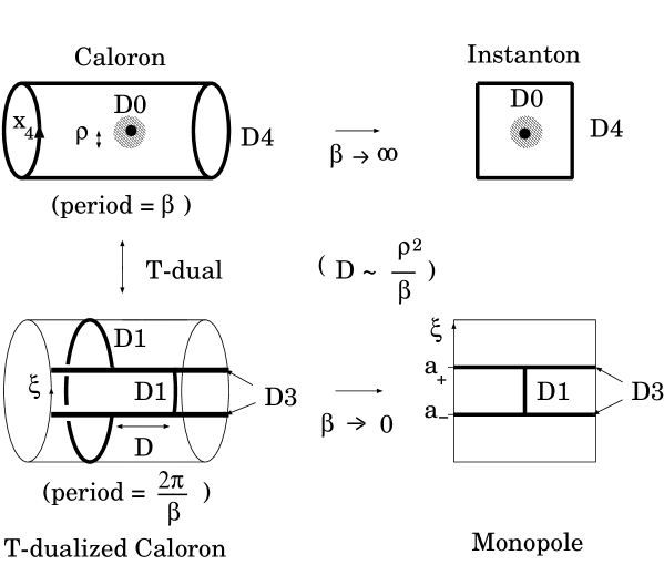
Figure 1: The D-brane description of $U(2)$ 1 caloron.

In the T-dualized picture, $U(N)$ 1 caloron can be interpreted as $N-1$ fundamental monopoles and the $N$-th monopole which appears from the Kaluza-Klein sector [34]. The value of the fourth component of the gauge field at spatial infinity on D4-brane determines the positions of the D3-branes which denote the Higgs expectation values of the monopole. The positions of the D3-branes are called the jumping points because at these points, the D1-brane is generally separated. In $N=2$ case, the separation interval (see figure 1) $D$ satisfies $D\sim\rho^{2}/\beta$ [34], [37], and if the size $\rho$ of periodic instanton is fixed and the period $\beta$ goes to zero, then one monopole decouples and the situation exactly coincides with that of PS-monopole [38]. BPS fluxons are represented as infinite D-strings piercing D3-branes in the background constant $B$-field and considered to be the T-dualized noncommutative calorons in the limit with the period $\beta\rightarrow 0$ and the interval $D\rightarrow 0$, which suggests $\rho=0$. (cf. figure 2)

Figure 2: The BPS fluxon

In the present paper, we give the various exact BPS solitons by ADHM/Nahm construction: localized instantons, localized calorons, localized doubly-periodic instantons and BPS fluxons which are essential in “solution generating technique.” The shift operators which play crucial roles in “solution generating technique” naturally appear in ADHM construction and other important points are all derived straightforwardly in ADHM/Nahm construction. In this way, we discuss the relationship between the two methods. The solutions of the localized calorons and the localized doubly-periodic instantons are new results. We also discuss a Fourier transformation of the localized calorons and show that the Fourier-transformed configurations of the localized calorons in the $\beta\rightarrow 0$ limit indeed coincides with BPS fluxons, which could be considered that BPS fluxons corresponding to D1-branes are the solitons of T-dualized solitons of localized calorons corresponding to D0-brane with the period $\beta\rightarrow 0$ up to space rotation [39], [40], [41].

This paper is organized as follows. In section 2, we briefly review “solution generating technique” and localized solitons. In section 3, we present ADHM construction of instantons and apply them to localized solitons. In section 4, we take the Fourier-transformation of the localized calorons and show that in the $\beta\rightarrow 0$ limit, the transformed solitons exactly coincide with BPS fluxons. Finally section 5 is devoted to conclusion and discussion.

2 A Review of “Solution Generating Technique” and Localized Solitons

In this section, we make a brief review of “solution generating technique” and some application of it which generates localized instantons and BPS fluxons.

Noncommutative gauge theories have two equivalent descriptions, that is, star-product formalism and operator formalism. There is a commutative description equivalent to the noncommutative gauge theories and the commutative and the noncommutative description are connected by Seiberg-Witten map [3]. In the present paper, we mainly use the operator formalism and when we make a physical interpretation, we shift to the commutative description by Seiberg-Witten map.

Let’s present noncommutative gauge theories in the operator formalism and establish notations. In this formalism, we start with the noncommutativity of the spatial coordinates (1.1) and define noncommutative gauge theories considering the coordinates as operators. From now on, we denote the hat on the operators in order to emphasize that they are operators. Here, for simplicity, we treat a noncommutative plane with the coordinates $\hat{x}^{1},\hat{x}^{2}$ which satisfy $[\hat{x}^{1},\hat{x}^{2}]=i\theta,~{}\theta>0$.

Defining new variables $\hat{a},\hat{a}^{\dagger}$ as

$$\hat{a}:=\frac{1}{\sqrt{2\theta}}\hat{z},~{}\hat{a}^{\dagger}:=\frac{1}{\sqrt{2\theta}}\hat{\bar{z}},$$ (2.1)

where $\hat{z}=\hat{x}^{1}+i\hat{x}^{2},~{}\hat{\bar{z}}=\hat{x}^{1}-i\hat{x}^{2}$, then we get the Heisenberg’s commutation relation:

$${[\hat{a},\hat{a}^{\dagger}]}=1.$$ (2.2)

Hence the spatial coordinates can be considered as the operators acting on Fock space ${\cal H}$ which is spanned by the occupation number basis $|n\rangle:=\left\{(\hat{a}^{\dagger})^{n}/\sqrt{n!}\right\}|0\rangle,~{}\hat{a}|0\rangle=0$:

$${\cal H}=\oplus_{n=0}^{\infty}{\bf C}|n\rangle.$$ (2.3)

The fields on the space depend on the spatial coordinates and are also the operators acting on the Fock space ${\cal H}$. They are represented by the occupation number basis as

$$\hat{f}=\sum_{m,n=0}^{\infty}f^{(mn)}|m\rangle\langle n|.$$ (2.4)

The matrix element $f^{(mn)}$ is infinite-size. If the fields has rotational symmetry on the plane, that is, the fields commute with the number operator $\hat{n}:=\hat{a}^{\dagger}\hat{a}\sim(\hat{x}^{1})^{2}+(\hat{x}^{2})^{2}$, they become diagonal:

$$\hat{f}=\sum_{n=0}^{\infty}f^{(n)}|n\rangle\langle n|.$$ (2.5)

The derivative of an operator $\hat{{\cal O}}$ can be defined by

$$\partial_{\mu}\hat{{\cal O}}:=[\hat{\partial}_{\mu},\hat{{\cal O}}],~{}~{}~{}~{}~{}~{}\mbox{where}~{}~{}~{}\hat{\partial}_{\mu}:=-i(\theta^{-1})_{\mu\nu}\hat{x}^{\nu},$$ (2.6)

which satisfies Leibniz rule and the desirable relation : $\partial_{\mu}\hat{x}^{\nu}=\delta_{\mu}^{~{}\nu}$. Moreover defining the following anti-Hermitian operator

$$\hat{D}_{\mu}:=\hat{\partial}_{\mu}+\hat{A}_{\mu},$$ (2.7)

where the $\hat{A}_{\mu}$ is a gauge field and anti-hermitian, then the covariant derivative of an adjoint field $\hat{\Phi}$ can be defined by $[\hat{D}_{\mu},\hat{\Phi}]$.

We note that using this anti-Hermitian operator $\hat{D}_{\mu}$, the field strength $\hat{F}_{\mu\nu}$ is rewritten as

$$\hat{F}_{\mu\nu}=[\hat{D}_{\mu},\hat{D}_{\nu}]-i(\theta^{-1})_{\mu\nu}.$$ (2.8)

Here the constant term $-i(\theta^{-1})_{\mu\nu}$ appears so that it should cancel out the term $[\hat{\partial}_{\mu},\hat{\partial_{\nu}}](=i(\theta^{-1})_{\mu\nu})$ in $[\hat{D}_{\mu},\hat{D}_{\nu}]$ and becomes an obstruct in applying “solution generating technique” to BPS equations.

From now on, we mainly use complex representations such as $\hat{D}_{z}:=(1/2)(\hat{D}_{1}-i\hat{D}_{2})=-(1/2\theta)\hat{\bar{z}}+\hat{A}_{z}$.

2.1 “Solution Generating Technique”

“Solution generating technique” is a transformation which leaves an equation as it is, that is, one of the auto-Bäcklund transformations. The transformation is almost a gauge transformation and defined as follows:

$$\hat{D}_{z}\rightarrow\hat{U}^{\dagger}\hat{D}_{z}\hat{U},$$ (2.9)

where $\hat{U}$ is an almost unitary operator and satisfies

$$\hat{U}\hat{U}^{\dagger}=1.$$ (2.10)

We note that we don’t put $\hat{U}^{\dagger}\hat{U}=1$. If $\hat{U}$ is finite-size, $\hat{U}\hat{U}^{\dagger}=1$ implies $\hat{U}^{\dagger}\hat{U}=1$ and then $\hat{U}$ and the transformation (2.9) become a unitary operator and just a gauge transformation respectively. Now, however, $\hat{U}$ is infinite-size and we only claim that $\hat{U}^{\dagger}\hat{U}$ is a projection because $(\hat{U}^{\dagger}\hat{U})^{2}=\hat{U}^{\dagger}(\hat{U}\hat{U}^{\dagger})\hat{U}=\hat{U}^{\dagger}\hat{U}$. The operator $\hat{U}$ which satisfies $\hat{U}\hat{U}^{\dagger}=1$ and $\hat{U}^{\dagger}\hat{U}=$ (projection) is often called the partial isometry.

The transformation (2.9) generally leaves an equation of motion as it is [26]:

$$\frac{\delta{\cal L}}{\delta{\cal O}}\rightarrow\hat{U}^{\dagger}\frac{\delta{\cal L}}{\delta{\cal O}}\hat{U},$$ (2.11)

where ${\cal L}$ and ${\cal O}$ are the Lagrangian and the field in the Lagrangian. Hence if one prepares a known solution of the equation of motion $\delta{\cal L}/\delta{\cal O}=0$, then we can get various new solution of it by applying the transformation (2.9) to the known solution.

The typical example of the partial isometry $\hat{U}$ is a shift operator. In $U(1)$ gauge theory, one of the shift operators acting on the Fock space (2.3) is

$$\hat{U}_{k}=\sum_{n=0}^{\infty}|n\rangle\langle n+k|,$$ (2.12)

which satisfies

$$\hat{U}_{k}\hat{U}_{k}^{\dagger}=1,~{}~{}~{}\hat{U}_{k}^{\dagger}\hat{U}_{k}=1-\hat{P}_{k},$$ (2.13)

where $\hat{P}_{k}$ is a projection onto the $k$-dimensional subspace of the Fock space ${\cal H}$ and expressed as

$$\hat{P}_{k}:=\sum_{m=0}^{k-1}|m\rangle\langle m|.$$ (2.14)

Here we note that in star product formalism, the behavior of the shift operator at large $|x|$ is order 1 which is denoted by ${\cal O}(1)$. The new soliton solutions from vacuum solutions are called localized solitons. The dimension of the projection $\hat{P}_{k}$ in fact represents the charge of the localized solitons. In general, the new solitons generated from known solitons by “solution generating technique” are the composite of known solitons and localized solitons.

“Solution generating technique” (2.9) can be generalized so as to include moduli parameters. In $U(1)$ gauge theory, the generalized transformation becomes as follows:

$$\hat{D}_{z}\rightarrow\hat{U}_{k}^{\dagger}\hat{D}_{z}\hat{U}_{k}-\sum_{m=0}^{k-1}\frac{\bar{\alpha}_{z}^{(m)}}{2\theta}|m\rangle\langle m|,$$ (2.15)

where $\alpha_{z}^{(m)}$ is an complex number and represents the position of the $m$-th localized soliton.

2.2 Localized Instantons

Localized instantons are obtained by applying “solution generating technique” (2.15) to the BPS equations of 4-dimensional noncommutative gauge theory.

First let’s consider the 4-dimensional noncommutative space with the coordinates $x^{\mu},~{}\mu=1,2,3,4$ whose noncommutativity is introduced as the canonical form:

$$\theta^{{\mu\nu}}=\left(\begin{array}[]{cccc}0&\theta_{1}&0&0\\ -\theta_{1}&0&0&0\\ 0&0&0&\theta_{2}\\ 0&0&-\theta_{2}&0\\ \end{array}\right).$$ (2.20)

The fields on the 4-dimensional noncommutative space whose noncommutativity is (2.20) are operators acting on Fock space ${\cal H}={\cal H}_{1}\otimes{\cal H}_{2}$ where ${\cal H}_{1}$ and ${\cal H}_{2}$ are defined by the same steps as the previous discussion corresponding to noncommutative $x_{1}$-$x_{2}$ plane and noncommutative $x_{3}$-$x_{4}$ plane respectively. The element in the Fock space ${\cal H}={\cal H}_{1}\otimes{\cal H}_{2}$ is denoted by $|n_{1}\rangle\otimes|n_{2}\rangle$ or $|n_{1},n_{2}\rangle$. We introduce the complex coordinates as $z_{1}=x_{1}+ix_{2},~{}z_{2}=x_{3}+ix_{4}$.

Here we make the noncommutative parameter $\theta^{\mu\nu}$ anti-self-dual: $\theta_{1}=-\theta_{2}=:\theta>0$, so that “solution generating technique” could work well on the BPS equation which is discussed later soon. In this case, we can define annihilation operators as $\hat{a}_{1}:=(1/\sqrt{2\theta})\hat{z}_{1},~{}\hat{a}_{2}:=(1/\sqrt{2\theta})\hat{\bar{z}}_{2}$ and creation operator $\hat{a}_{1}^{\dagger}:=(1/\sqrt{2\theta})\hat{\bar{z}}_{1},~{}\hat{a}_{2}^{\dagger}:=(1/\sqrt{2\theta})\hat{z}_{2}$ in Fock space ${\cal H}=\oplus_{n_{1},n_{2}=0}^{\infty}{\bf C}|n_{1}\rangle\otimes|n_{2}\rangle$ such as

$$[\hat{a}_{1},\hat{a}_{1}^{\dagger}]=1,~{}[\hat{a}_{2},\hat{a}_{2}^{\dagger}]=1,~{}\mbox{otherwise}=0,$$ (2.21)

where $|n_{1}\rangle$ and $|n_{2}\rangle$ are the occupation number basis generated form the vacuum state $|0\rangle$ by the action of $\hat{a}_{1}^{\dagger}$ and $\hat{a}_{2}^{\dagger}$ respectively.

4-dimensional noncommutative gauge theory is defined by the pure Yang-Mills action:

$${\cal L}_{\scriptsize\mbox{YM}}=-\frac{1}{4g^{2}_{\scriptsize\mbox{YM}}}\int d^{4}x~{}{\rm Tr}F_{\mu\nu}F^{\mu\nu},$$ (2.22)

where $\int d^{4}x$ denotes ${\rm Tr}_{{\cal H}}$.

The anti-self-dual BPS equations are obtained as the condition that the action density should take the minimum:

$$(\hat{F}_{z_{1}\bar{z}_{1}}+\hat{F}_{z_{2}\bar{z}_{2}}=) -[\hat{D}_{z_{1}},\hat{D}_{z_{1}}^{\dagger}]-[\hat{D}_{z_{2}},\hat{D}_{z_{2}}^{\dagger}]-\frac{1}{2}\left(\frac{1}{\theta_{1}}+\frac{1}{\theta_{2}}\right)=0,$$

$$(\hat{F}_{z_{1}z_{2}}=) [\hat{D}_{z_{1}},\hat{D}_{z_{2}}]=0,$$ (2.23)

The fields are denoted by the occupation number basis as

$$\hat{A}_{\mu}(\hat{x}) = \sum_{m_{1},m_{2},n_{1},n_{2}=0}^{\infty}c_{\mu}^{(m_{1},m_{2},n_{1},n_{2})}|m_{1},m_{2}\rangle\langle n_{1},n_{2}|$$ (2.24)

$$= \sum_{m_{1},m_{2},n_{1},n_{2}=0}^{\infty}c_{\mu}^{(m_{1},m_{2},n_{1},n_{2})}|m_{1}\rangle\langle n_{1}|\otimes|m_{2}\rangle\langle n_{2}|,$$

where $c_{\mu}^{(m_{1},m_{2},n_{1},n_{2})}$ is a number. We note that only when noncommutative parameter $\theta^{ij}$ is anti-self-dual, the constant term $\left(1/\theta_{1}+1/\theta_{2}\right)$ disappears and “solution generating technique” can leave the BPS equation (2.2) as it is.

Localized instanton solutions are generated by “solution generating technique” from the vacuum solution which trivially satisfies the BPS equation (2.2) and given by

$$\hat{D}_{z_{i}}=\hat{U}_{k}^{\dagger}\hat{\partial}_{z_{i}}\hat{U}_{k}-\sum_{m=0}^{k-1}\frac{\bar{\alpha}_{i}^{(m)}}{2\theta_{i}}|0,m\rangle\langle 0,m|,$$ (2.25)

where the shift operators can be taken for example as [42]

$$\hat{U}_{k}=\sum_{n_{1}=1,n_{2}=0}^{\infty}|n_{1},n_{2}\rangle\langle n_{1},n_{2}|+\sum_{n_{2}=0}^{\infty}|0,n_{2}\rangle\langle 0,n_{2}+k|,$$ (2.26)

which satisfies

$$\hat{U}_{k}\hat{U}_{k}^{\dagger}=1,~{}~{}~{}\hat{U}_{k}^{\dagger}\hat{U}_{k}=1-\sum_{m=0}^{k-1}|0\rangle\langle 0|\otimes|m\rangle\langle m|.$$ (2.27)

The field strength and the instanton number $\nu[\hat{A}]$ are calculated as

$$\hat{F}_{\mu\nu} = -i(\theta^{-1})_{\mu\nu}|0\rangle\langle 0|\otimes\hat{P}_{k},$$ (2.28)

$$\nu[\hat{A}] := \frac{1}{16\pi^{2}}\int d^{4}x~{}\hat{F}_{\mu\nu}\hat{F}^{\mu\nu}=-\dim_{{\cal H}}|0\rangle\langle 0|\otimes\hat{P}_{k}=-k$$ (2.29)

Therefore the existence of the non-trivial projection $\hat{P}_{k}$ is crucial in generating localized solitons and the dimension of the projection corresponds to the instanton number.

The interpretation of the moduli parameter $\alpha_{i}^{(m)}$ is clear in commutative description. The exact Seiberg-Witten map [43] of the solution (2.25) is obtained in [44] and the D0-brane density is

$$J_{\scriptsize\mbox{D0}}(x)=\frac{2}{\theta^{2}}+\sum_{m=0}^{k-1}\delta(x_{1}-\lambda_{1}^{(m)})\delta(x_{2}-\lambda_{2}^{(m)})\delta(x_{3}-\lambda_{3}^{(m)})\delta(x_{4}-\lambda_{4}^{(m)}),$$ (2.30)

where the real parameters $\lambda_{\mu}^{(m)}$ are the real or the imaginary part of $\alpha_{i}^{(m)}$, that is, $\alpha_{1}^{(m)}=\lambda_{1}^{(m)}+i\lambda_{2}^{(m)},~{}\alpha_{2}^{(m)}=\lambda_{3}^{(m)}+i\lambda_{4}^{(m)}$. The first term and the second term of the right hand side in (2.30) show the uniform distribution of the D0-branes on D4-brane and localized $k$-D0-brane charge respectively, which represents just the $k$-localized instantons. The moduli parameter $\alpha_{i}^{(m)}$ or $\lambda_{\mu}^{(m)}$ are clearly interpreted as the positions of the localized instantons.

2.3 BPS Fluxons

BPS fluxons are obtained by applying “solution generating technique” to the BPS equation of $(3+1)$-dimensional noncommutative gauge theory with the coordinates $(x^{0},x^{i}),~{}i=1,2,3$ whose noncommutativity is $\theta^{12}=\theta>0$.

$(3+1)$-dimensional noncommutative gauge theory is defined by the Yang-Mills-Higgs action:

$$I_{\scriptsize\mbox{YMH}}=-\frac{1}{4g^{2}_{\scriptsize\mbox{YM}}}\int d^{4}x~{}{\rm Tr}\left(\hat{F}_{{\mu\nu}}\hat{F}^{{\mu\nu}}+2[\hat{D}_{\mu},\hat{\Phi}][\hat{D}_{\mu},\hat{\Phi}]\right),$$ (2.31)

where $\hat{\Phi}$ is an adjoint Higgs field and $\int dx_{1}dx_{2}$ denotes ${\rm Tr}_{{\cal H}}$. The anti-self-dual BPS equations are obtained as subsection 2.2:

$$(\hat{B}_{3}=) [\hat{D}_{z},\hat{D}_{z}^{\dagger}]+\frac{1}{\theta}=-[\hat{D}_{3},\hat{\Phi}],$$

$$(\hat{B}_{z}=) [\hat{D}_{3},\hat{D}_{z}]=-[\hat{D}_{z},\hat{\Phi}],$$ (2.32)

where $\hat{B}_{i}$ are magnetic fields. This equation is often called Bogomol’nyi equation [45]. The fields with rotational symmetry on $x_{1}$-$x_{2}$ plane are denoted by the occupation number basis as

$$\hat{\Phi}=\sum_{n=0}^{\infty}\Phi^{(n)}(x_{3})|n\rangle\langle n|,~{}~{}~{}\hat{A}=\sum_{n=0}^{\infty}A^{(n)}(x_{3})|n\rangle\langle n|.$$ (2.33)

Because of the constant term in the left hand side of the first equation of (2.3), “solution generating technique” (2.15) cannot work. The modified “solution generating technique” which leaves the BPS equation (2.3) as it is is found in [27], [28]:

$$\hat{\Phi} \rightarrow \hat{U}_{k}^{\dagger}\hat{\Phi}\hat{U}_{k}-\frac{x_{3}}{\theta}\hat{P}_{k}+\sum_{m=0}^{k-1}\lambda^{(m)}_{\Phi}|m\rangle\langle m|,$$

$$\hat{D}_{3} \rightarrow \partial_{3}+\hat{U}_{k}^{\dagger}\hat{A}_{3}\hat{U}_{k}-i\sum_{m=0}^{k-1}\frac{\lambda^{(m)}_{4}}{\theta}|m\rangle\langle m|,$$

$$\hat{D}_{z} \rightarrow \hat{U}^{\dagger}_{k}\hat{D}_{z}\hat{U}_{k}-\sum_{m=0}^{k-1}\frac{\bar{\alpha}^{(m)}_{z}}{2\theta}|m\rangle\langle m|,$$ (2.34)

where $\hat{U}_{k}$ and $\hat{P}_{k}$ are the same as (2.12) and (2.14) respectively. The important modification is to add the linear term of $x_{3}$ to the transformation of the Higgs field $\hat{\Phi}$. The localized soliton solutions in this theory are generated from the vacuum solution by the transformation (2.3)

$$\hat{\Phi} = -\sum_{m=0}^{k-1}\left(\frac{x_{3}}{\theta}-\lambda_{\Phi}^{(m)}\right)|m\rangle\langle m|,$$

$$\hat{D}_{z} = \hat{U}^{\dagger}_{k}\hat{\partial}_{z}\hat{U}_{k}-\sum_{m=0}^{k-1}\frac{\alpha_{z}^{(m)}}{2\theta}|m\rangle\langle m|,~{}~{}~{}\hat{A}_{3}=-i\sum_{m=0}^{k-1}\frac{\lambda_{4}^{(m)}}{\theta}|m\rangle\langle m|,$$

$$\hat{B}_{3} = \frac{1}{\theta}\hat{P}_{k},~{}~{}~{}\hat{B}_{1}=\hat{B}_{2}=0,$$ (2.35)

which is called the BPS fluxon [11], [12] because this is similar to a flux-tube rather than a monopole.

The D1-brane density in commutative side is obtained by Seiberg-Witten map in [44]:

$$J_{\scriptsize\mbox{D1}}(x)=\frac{1}{\theta}\delta(\Phi)+\sum_{m=0}^{k-1}\delta(x_{1}-\lambda_{1}^{(m)})\delta(x_{2}-\lambda_{2}^{(m)})\delta(\Phi+(x_{3}-\lambda_{3}^{(m)})/\theta).$$ (2.36)

Hence the parameter $\lambda_{i}^{(m)}$ shows the positions of BPS fluxon and here we use the relation $\lambda_{\Phi}=\lambda_{3}/\theta$ (cf. figure 2). We can take $\lambda_{4}^{(m)}=0$ because $\lambda_{4}^{(m)}$ doesn’t appear in (2.36) and has no physical meaning.

3 ADHM/Nahm Construction of Localized Solitons

In this section, we first review ADHM construction of commutative instantons and then apply it to localized instantons, localized periodic instantons (=localized calorons), localized doubly-periodic instantons and BPS fluxons. The procedure of the constructions are the same as the commutative case and gives rise to various exact BPS solitons straightforwardly. The shift operators and moduli terms naturally appear in ADHM construction of localized instantons, and the linear term of $x_{3}$ in (2.3) is necessarily obtained in Nahm construction of BPS fluxons. The localized calorons and the localized doubly-periodic instantons are new solitons.

3.1 A Review of ADHM Construction of Instantons and Calorons

In this subsection, we discuss ADHM construction of commutative instantons. First let’s introduce the Euclidean 4-dimensional Pauli matrices:

$$e_{\mu}:=(-i\sigma_{i},1),~{}~{}~{}e_{\mu}^{\dagger}=(i\sigma_{i},1),$$ (3.1)

which correspond to the basis of the quarternion as algebra : $e_{i}e_{j}=-\delta_{ij}+\epsilon_{ijk}e_{k}$ and also satisfy the following relations:

$$e_{\mu}e_{\nu}^{\dagger} = \delta_{\mu\nu}+i\eta_{\mu\nu}^{i(-)}\otimes\sigma_{i},$$

$$e_{\mu}^{\dagger}e_{\nu} = \delta_{\mu\nu}+i\eta_{\mu\nu}^{i(+)}\otimes\sigma_{i}.$$ (3.2)

Here $\eta_{\mu\nu}^{i(\pm)}$ are called ’t Hooft symbol and concretely represented as

$$\eta^{i(\pm)}_{\mu\nu}=\epsilon_{i{\mu\nu}4}\pm\delta_{i\mu}\delta_{\nu 4}\mp\delta_{i\nu}\delta_{\mu 4}.$$ (3.3)

These symbols are anti-symmetric and (anti-)self-dual. Next we define “0-dimensional Dirac operator” which is $(N+2k)\times 2k$ matrix as

$$\hat{\nabla} := \left(\begin{array}[]{c}S\\ (x^{\mu}-T^{\mu})\otimes e^{\mu}\end{array}\right)=\left(\begin{array}[]{cc}J&I^{\dagger}\\ -i(z_{2}-B_{2})&-i(\bar{z}_{1}-B_{1}^{\dagger})\\ -i(z_{1}-B_{1})&i(\bar{z}_{2}-B_{2}^{\dagger})\end{array}\right),$$ (3.9)

where $S$ and $T_{\mu}$ are $N\times 2k$ and $k\times k$ matrices respectively and $T_{\mu}$ are Hermitian : $T_{\mu}^{\dagger}=T_{\mu}$. $I$ and $J$ are $k\times N$ and $N\times k$ matrices respectively and $B_{1}:=T_{1}+iT_{2},~{}B_{2}:=T_{3}+iT_{4}$.

The matrices satisfy the following relations which is equivalent to that $\nabla^{\dagger}\nabla$ commute with Pauli matrices $\sigma_{i}$:

$${[B_{1},B_{1}^{\dagger}]}+[B_{2},B_{2}^{\dagger}]+II^{\dagger}-J^{\dagger}J~{}(\equiv-[z_{1},\bar{z}_{1}]-[z_{2},\bar{z}_{2}])=0,$$

$${[B_{1},B_{2}]}+IJ=0,$$ (3.10)

which are called ADHM equations. Moreover we have to put another condition on the matrices that $\nabla^{\dagger}\nabla$ is invertible, which is in fact necessary in ADHM construction.

ADHM construction consists of the following three steps. The first step is to solve the ADHM equations. Next step is to solve the following “0-dimensional Dirac equation” in the background of the solution of ADHM eq. (3.1):

$$\nabla^{\dagger}V=0,$$ (3.11)

where $V$ is $(N+2k)\times N$ matrices and satisfies the normalization condition:

$$V^{\dagger}V=1,$$ (3.12)

and completeness condition:

$$VV^{\dagger}=1-\nabla(\nabla^{\dagger}\nabla)^{-1}\nabla^{\dagger}.$$ (3.13)

which comes from the assumption that $\nabla^{\dagger}\nabla$ is invertible. It is convenient to introduce the following decomposed matrices of $V$ :

$$V=\left(\begin{array}[]{c}u\\ v\end{array}\right)=\left(\begin{array}[]{c}u\\ v_{1}\\ v_{2}\end{array}\right),$$ (3.19)

where $u,v$ and $v_{1,2}$ are $N\times N,~{}2k\times N$ and $k\times N$ matrices respectively. We note that $u$ and $v$ behave ${\cal O}(1)$ and ${\cal O}(r^{-1})$ at $r=|x|\rightarrow\infty$ respectively [48]. The final step is to construct the (anti-)self-dual gauge fields using the solution $V$ of the “0-dimensional Dirac equation” (3.11) as follows:

$$A_{\mu} = V^{\dagger}\partial_{\mu}V=u^{\dagger}\partial_{\mu}u+v^{\dagger}\partial_{\mu}v.$$ (3.20)

The field strength is calculated from the gauge fields:

$$F = dA+A\wedge A$$ (3.21)

$$= dV^{\dagger}\wedge dV+V^{\dagger}dV\wedge V^{\dagger}dV=dV^{\dagger}\wedge dV-dV^{\dagger}V\wedge V^{\dagger}dV$$

$$= dV^{\dagger}(1-VV^{\dagger})\wedge dV=dV^{\dagger}\nabla(\nabla^{\dagger}\nabla)^{-1}\nabla^{\dagger}\wedge dV$$

$$= V^{\dagger}(d\nabla)(\nabla^{\dagger}\nabla)^{-1}\wedge(d\nabla^{\dagger})V=v^{\dagger}e_{\mu}dx^{\mu}(\nabla^{\dagger}\nabla)^{-1}\wedge e^{\dagger}_{\nu}dx^{\nu}v$$

$$= iv^{\dagger}(\nabla^{\dagger}\nabla)^{-1}\eta^{(-)}_{\mu\nu}vdx^{\mu}\wedge dx^{\nu}.$$

$$F_{\mu\nu} = 2iv^{\dagger}(\nabla^{\dagger}\nabla)^{-1}\eta^{(-)}_{\mu\nu}v.$$ (3.22)

Hence anti-self-dual gauge fields have been constructed. In the last line of the equation (3.21), we use the condition that $\nabla^{\dagger}\nabla$ should commute with Pauli matrices.

$G=SU(2)$ ’t Hooft $k$ instantons

Let’s construct $G=SU(2)$ ’t Hooft $k$-instanton solution following the steps in ADHM construction. The solution of ADHM equation (3.1) is simply given for this instanton as follows:

$$S = \left(\begin{array}[]{ccc}\begin{array}[]{cc}\rho_{1}&0\\ 0&\rho_{1}\end{array}&\cdots&\begin{array}[]{cc}\rho_{k}&0\\ 0&\rho_{k}\end{array}\end{array}\right),$$ (3.28)

$$T_{\mu} = \mbox{diag}\,_{m=0}^{k-1}(\lambda_{\mu}^{(m)}),$$ (3.29)

where the symbol “diag ” denotes diagonal sum and $\lambda_{\mu}^{(m)}$ and $\rho_{m}$ are real numbers. “0-dimensional Dirac equation” (3.11) is also simply solved:

$$V=\frac{1}{\sqrt{{\cal N}}}\left(\begin{array}[]{c}1\\ -((x^{\mu}-T^{\mu})\otimes e^{\dagger}_{\mu})^{-1}S^{\dagger}\end{array}\right),$$ (3.32)

where the normalization factor ${\cal N}$ is determined by normalization condition (3.12) as

$${\cal N}=1+\sum_{m=0}^{k-1}\frac{\rho_{m}^{2}}{|x-\lambda^{(m)}|^{2}},$$ (3.33)

and

$$((x^{\mu}-T^{\mu})\otimes e^{\dagger}_{\mu})^{-1}=\mbox{diag}\,_{m=0}^{k-1}\left(\frac{(x_{\mu}-\lambda_{\mu}^{(m)})}{|x-\lambda^{(m)}|^{2}}\otimes e^{\mu}\right).$$ (3.34)

$\hat{u}$ and $\hat{v}$ are actually ${\cal O}(1)$ and ${\cal O}(r^{-1})$ respectively. The gauge fields are given by

$$A_{\mu} = V^{\dagger}\partial_{\mu}V=-\frac{i}{{\cal N}}\sum_{m=0}^{k-1}\frac{\rho_{m}^{2}\eta_{\mu\nu}^{(+)}(x_{\nu}-\lambda_{\nu}^{(m)})}{|x-\lambda^{(m)}|^{4}}=-\frac{i}{2}\eta_{\mu\nu}^{(+)}\partial^{\nu}\log{\cal N}.$$ (3.35)

This solution is called ’t Hooft-instanton solution and singular at $x=\lambda^{(m)}$, which results from that a singular gauge is taken.

$G=SU(2)$ 1 caloron

The solution (3.35) can be generalized to periodic-instanton solution. We can take the instanton number $k=\infty$ and all the size of the instantons $\rho_{m}=\rho$ and put them periodically along the $x_{4}$ axis where the period is $\beta$. This soliton is called the caloron [31] and then ${\cal N}$ becomes

$${\cal N}=1+\sum_{m=-\infty}^{\infty}\frac{\rho^{2}}{|x-m\beta x_{4}|^{2}}=1+\frac{\pi\rho^{2}}{\beta|\vec{x}|}\frac{\sinh\left(\displaystyle\frac{2\pi}{\beta}|\vec{x}|\right)}{\cosh\left(\displaystyle\frac{2\pi}{\beta}|\vec{x}|\right)-\cos\left(\displaystyle\frac{2\pi}{\beta}x_{4}\right)},$$ (3.36)

where $\vec{x}=(x_{1},x_{2},x_{3})$.

The caloron solution coincides with PS-monopole solution [38] up to gauge transformation with $\beta\rightarrow 0$. PS-monopole solution is given by

$$\Phi = -\frac{x^{i}\sigma_{i}}{|\vec{x}|^{2}}\left(\frac{a|\vec{x}|}{\tanh a|\vec{x}|}-1\right),$$

$$A_{i} = \frac{\epsilon_{ijk}\sigma^{j}x^{k}}{|\vec{x}|^{2}}\left(\frac{a|\vec{x}|}{\sinh a|\vec{x}|}-1\right),$$ (3.37)

where the real constant $a$ represents the vacuum expectation value of the Higgs field, which appears in the gauge transformation. This is reinterpreted clearly from D-brane picture in [34]. (cf. figure 1.) We will discuss the similar discussion about localized caloron solution in section 4.

3.2 ADHM Construction of Localized Instantons and Calorons

Now let’s generalize the above discussion to noncommutative case. The difference to commutative case is that the coordinates are operators which act on the Fock space. ADHM equation is deformed by the noncommutativity of the spatial coordinates as follows:

$${[B_{1},B_{1}^{\dagger}]}+[B_{2},B_{2}^{\dagger}]+II^{\dagger}-J^{\dagger}J=-2(\theta_{1}+\theta_{2}),$$

$${[B_{1},B_{2}]}+IJ=0.$$ (3.38)

We note that the constant term in the right hand side of the first equation disappears only when the noncommutative parameter is anti-self-dual, that is, $\theta_{1}+\theta_{2}=0$, which is necessary for the existence of the localized instantons.

The steps to give rise to instantons are the same as the commutative case.

localized $U(1)~{}k$ instantons

Now let’s find localized $U(1)$ instanton solutions using ADHM construction, which is considered as the noncommutative version of the ’t Hooft instanton solution in the $\rho^{(m)}\rightarrow 0$ limit.

ADHM equations (3.2) are simply solved and the solution of them for localized instantons is

$$I=J=0,~{}~{}~{}B_{1}=\mbox{diag}\,_{m=0}^{k-1}(\alpha_{1}^{(m)}),~{}~{}~{}B_{2}=\mbox{diag}\,_{m=0}^{k-1}(\alpha_{2}^{(m)}),$$ (3.39)

where $\alpha_{i}^{(m)}$ should show the position of the $m$-th instanton because $B_{1,2}$ is the scalar field on D0-branes. $I$ and $J$ contain the information of the size of instantons and hence $I=J=0$ characterize the localized instantons because localized instantons have no moduli parameter of the size and singular on commutative side as (2.30).

Next we solve “0-dimensional Dirac equation” in the background of the solutions (3.39) of the ADHM equation. This is also simple. Observing the right hand side of the complete condition (3.13), we get $\hat{v}_{1}^{(m)}=|\alpha^{(m)}_{1},\alpha^{(m)}_{2}\rangle\langle p_{1}^{(m)},p_{2}^{(m)}|$ and $\hat{v}_{2}=0$, where $|p_{1}^{(m)},p_{2}^{(m)}\rangle$ is the normalized orthogonal state in ${\cal H}_{1}\otimes{\cal H}_{2}$:

$$\langle p_{1}^{(m)},p_{2}^{(m)}|p_{1}^{(n)},p_{2}^{(n)}\rangle=\delta_{mn},$$ (3.40)

and $|\alpha^{(m)}_{1},\alpha^{(m)}_{2}\rangle$ is the normalized coherent state and satisfies

$$\hat{z}_{1}|\alpha^{(m)}_{1},\alpha^{(m)}_{2}\rangle=\alpha^{(m)}_{1}|\alpha^{(m)}_{1},\alpha^{(m)}_{2}\rangle,$$

$$\hat{\bar{z}}_{2}|\alpha^{(m)}_{2},\alpha^{(m)}_{2}\rangle=\bar{\alpha}^{(m)}_{2}|\alpha^{(m)}_{1},\alpha^{(m)}_{2}\rangle,$$

$$\langle\alpha^{(m)}_{1},\alpha^{(m)}_{2}|\alpha^{(m)}_{1},\alpha^{(m)}_{2}\rangle=1.$$ (3.41)

The eigen values $\alpha^{(m)}_{1}$ and $\alpha_{2}^{(m)}$ of $\hat{z}_{1}$ and $\hat{\bar{z}}_{2}$ are decided to be just the same as the $m$-th diagonal components of the solution $B_{1},B_{2}$ in (3.39). Though $\hat{u}$ is undetermined, $\hat{V}$ already satisfies $\nabla^{\dagger}\hat{V}=0$, which comes from that in the case that the self-duality of gauge fields and noncommutative parameter are the same, the coordinates in each column of $\nabla^{\dagger}$ play the same role in the sense that they are annihilation operators or creation operators.

The last condition is the normalization condition (3.12) and determines $\hat{u}=\hat{U}_{k}$ where $\hat{U}_{k}\hat{U}_{k}^{\dagger}=1,~{}\hat{U}_{k}^{\dagger}\hat{U}_{k}=1-\hat{P}_{k}=1-\sum_{m=0}^{k-1}|p_{1}^{(m)},p_{2}^{(m)}\rangle\langle p_{1}^{(m)},p_{2}^{(m)}|$. This is just the shift operator and naturally appears in this way. The shift operator and $\hat{u}$ have the same behavior at $|x|\rightarrow\infty$ and this is consistent.

Gathering the results, the solution of (3.11) is

$$\hat{V}=\left(\begin{array}[]{c}\hat{u}\\ \hat{v}_{1}^{(m)}\\ \hat{v}_{2}^{(m)}\end{array}\right)=\left(\begin{array}[]{c}\hat{U}_{k}\\ |\alpha^{(m)}_{1},\alpha^{(m)}_{2}\rangle\langle p_{1}^{(m)},p_{2}^{(m)}|\\ 0\end{array}\right),$$ (3.48)

where $\hat{v}_{i}^{(m)}$ is the $m$-th low of $\hat{v}_{i}$. This is the general form of the solution of “0-dimensional Dirac equation” and gives rise to localized instanton solution:

$$\hat{A}_{z_{i}} = \hat{V}^{\dagger}[\hat{\partial}_{z_{i}},\hat{V}]=\hat{u}^{\dagger}\hat{\partial}_{z_{i}}\hat{u}+\hat{v}^{\dagger}\hat{\partial}_{z_{i}}\hat{v}-\hat{\partial}_{z_{i}}$$ (3.49)

$$= \hat{U}_{k}^{\dagger}\hat{\partial}_{z_{i}}\hat{U}_{k}-|p_{1}^{(m)},p_{2}^{(m)}\rangle\langle\alpha^{(m)}_{1},\alpha^{(m)}_{2}|\frac{\hat{\bar{z}}_{i}}{2\theta^{i}}|\alpha^{(m)}_{1},\alpha^{(m)}_{2}\rangle\langle p_{1}^{(m)},p_{2}^{(m)}|-\hat{\partial}_{z_{i}}$$

$$= \hat{U}_{k}^{\dagger}\hat{\partial}_{z_{i}}\hat{U}_{k}-\hat{\partial}_{z_{i}}-\sum_{m=0}^{k-1}\frac{\bar{\alpha}_{z_{i}}^{(m)}}{2\theta^{i}}|p_{1}^{(m)},p_{2}^{(m)}\rangle\langle p_{1}^{(m)},p_{2}^{(m)}|.$$

If $|p_{1}^{(m)},p_{2}^{(m)}\rangle=|0,m\rangle$ and $\hat{U}_{k}$ is the same as (2.26), then the gauge fields is the same as (2.25).

The solution $\hat{V}$ of “0-dimensional Dirac equation” also contains all informations of the instantons. The instanton number $k$ is represented by the dimension of the projected states$|p_{1}^{(m)},p_{2}^{(m)}\rangle$ which appears in the relations of the shift operator $\hat{u}=\hat{U}_{k}$ or the bra part of $\hat{v}_{1}^{(m)}$ The information of the position of $k$ localized solitons is shown in the coherent state $|\alpha_{i}^{(m)}\rangle$ in the ket part of $\hat{v}_{1}^{(m)}$.

localized $U(1)$ 1 caloron

Now let’s construct a localized caloron solution as commutative caloron solution in subsection 3.1, that is, we take the instanton number $k\rightarrow\infty$ and put infinite number of localized instantons in the $x_{4}$ direction at regular intervals. We have to find an appropriate shift operator so that it gives rise to an infinite-dimensional projection operator and put the moduli parameter $\lambda_{4}$ periodic.

The solution is found as:

$$\hat{A}_{z_{1}} = \hat{U}_{k\times\infty}^{\dagger}\hat{\partial}_{z_{1}}\hat{U}_{k\times\infty}-\hat{\partial}_{z_{1}}-\sum_{m=0}^{k-1}\frac{\bar{\alpha}_{1}^{(m)}}{2\theta}|m\rangle\langle m|\otimes 1_{{\cal H}_{2}},$$

$$\hat{A}_{z_{2}} = \hat{U}_{k\times\infty}^{\dagger}\hat{\partial}_{z_{2}}\hat{U}_{k\times\infty}-\hat{\partial}_{z_{2}}+\sum_{m=0}^{k-1}\sum_{n=-\infty}^{\infty}\frac{\bar{\alpha}_{2}^{(m)}-in\beta}{2\theta}|m\rangle\langle m|\otimes|n\rangle\langle n|,$$ (3.50)

where the shift operator is defined as

$$\hat{U}_{k\times\infty}=\sum_{n_{1}=0}^{\infty}|n_{1}\rangle\langle n_{1}+k|\otimes 1_{{\cal H}_{2}}.$$ (3.51)

The field strength is calculated as

$$\hat{F}_{12}=-\hat{F}_{34}=i\frac{1}{\theta}\hat{P}_{k}\otimes 1_{{\cal H}_{2}},$$ (3.52)

which is trivially periodic in the $x_{4}$ direction. It seems to be strange that this contains no information of the period $\beta$. Hence one may wonder if this solution is the charge-one caloron solution on ${\bf R}^{3}\times S^{1}$ whose perimeter is $\beta$. Moreover one may doubt if this suggests that this soliton represents D2-brane not infinite number of D0-branes.

The apparent paradox is solved by mapping this solution to commutative side by exact Seiberg-Witten map. The commutative description of D0-brane density is as follows

$$J_{\scriptsize\mbox{D0}}(x)=\frac{2}{\theta^{2}}+\sum_{m=0}^{k-1}\sum_{n=-\infty}^{\infty}\delta(x_{1}-\lambda_{1}^{(m)})\delta(x_{2}-\lambda_{2}^{(m)})\delta(x_{3}-\lambda_{3}^{(m)})\delta(x_{4}-\lambda_{4}^{(m)}-n\beta).$$ (3.53)

The information of the period has appeared and the solution (3.2) is shown to be an appropriate charge-one caloron solution with the period $\beta$. The above paradox is due to the fact that in noncommutative gauge theories, there is no local observable and the period becomes obscure. And as is pointed out in [44], the D2-brane density is exactly zero. Hence the paradox has been solved clearly.

This soliton can be interpreted as a localized instanton on noncommutative ${\bf R}^{3}\times S^{1}$.

localized $U(1)$ 1 doubly-periodic instantons

In similar way, we can construct doubly-periodic (in the $x_{3}$ and $x_{4}$ directions) instanton solution:

$$\hat{A}_{z_{1}} = \hat{U}_{k\times\infty}^{\dagger}\hat{\partial}_{z_{1}}\hat{U}_{k\times\infty}-\hat{\partial}_{z_{1}}-\sum_{m=0}^{k-1}\frac{\bar{\alpha}_{1}^{(m)}}{2\theta}|m\rangle\langle m|\otimes 1_{{\cal H}_{2}},$$

$$\hat{A}_{z_{2}} = \hat{U}_{k\times\infty}^{\dagger}\hat{\partial}_{z_{2}}\hat{U}_{k\times\infty}-\hat{\partial}_{z_{2}}$$ (3.54)

$$+\sum_{m=0}^{k-1}\sum_{n_{1},n_{2}=-\infty}^{\infty}\frac{\bar{\alpha}_{2}^{(m)}+\beta_{1}n_{1}-i\beta_{2}n_{2}}{2\theta}|m\rangle\langle m|\otimes|\widetilde{\alpha}_{n_{1}n_{2}}^{(l_{1},l_{2})}\rangle\langle\widetilde{\alpha}_{n_{1}n_{2}}^{(l_{1},l_{2})}|,$$

where the system $\left\{|\widetilde{\alpha}^{(l_{1},l_{2})}_{n_{1},n_{2}}\rangle\right\}_{n_{1},n_{2}\in\scriptsize{\bf Z}}$ is von Neumann lattice [50] and an orthonormal and complete set [51], [52]. Von Neumann lattice is the complete subsystem of the set of the coherent states which is over-complete, and generated by $e^{l_{1}\hat{\partial}_{3}}$ and $e^{l_{2}\hat{\partial}_{4}}$, where the periods of the lattice $l_{1},l_{2}\in{\bf R}$ satisfies $l_{1}l_{2}=2\pi\theta$. (See also [53], [54].) This complete system has two kind of labels and suitable to doubly-periodic instanton. Of course, another complete system can be available if one label the system appropriately.

The field strength in the noncommutative side is the same as (3.52) and the commutative description of D0-brane density becomes

$$J_{\scriptsize\mbox{D0}}(x) = \frac{2}{\theta^{2}}+\sum_{m=0}^{k-1}\sum_{n_{1},n_{2}=-\infty}^{\infty}\delta(x_{1}-\lambda_{1}^{(m)})\delta(x_{2}-\lambda_{2}^{(m)})\times$$ (3.55)

$$~{}~{}~{}~{}~{}~{}~{}~{}~{}~{}~{}~{}~{}~{}~{}~{}~{}~{}~{}~{}~{}~{}~{}\delta(x_{3}-\lambda_{3}^{(m)}-n_{1}\beta_{1})\delta(x_{4}-\lambda_{4}^{(m)}-n_{2}\beta_{2}),$$

which guarantees that this is an appropriate charge-one doubly-periodic instanton solution with the period $\beta_{1},\beta_{2}$.

This soliton can be interpreted as a localized instanton on noncommutative ${\bf R}^{2}\times T^{2}$. The exact known solitons on noncommutative torus are very refined or abstract as is found in [54], [55], [56], [57]. It is therefore notable that our simple solution (3.2) is indeed doubly-periodic. The point is that we treat noncommutative ${\bf R}^{4}$ not noncommutative torus and apply “solution generating technique” to ${\cal H}_{1}$ side only.

localized $U(N)~{}k$ instantons

There is an obvious generalization of the construction of $U(N)$ localized instanton as follows. In the solution of ADHM equations, $I,J$ can be still zero and $B_{1,2}$ are the same as that of $N=1$ case. The solution of “0-dimensional Dirac equation” (3.11) is given by

$$\hat{V}=\left(\begin{array}[]{c}\hat{u}\\ \hat{v}_{1}^{(m,a)}\\ \hat{v}_{2}^{(m,a)}\end{array}\right)=\left(\begin{array}[]{c}\hat{U}_{k}\\ |\alpha^{(m_{a})}_{1},\alpha^{(m_{a})}_{2}\rangle\langle p_{1}^{(m_{a})},p_{2}^{(m_{a})}|\\ 0\end{array}\right),$$ (3.62)

where $m_{a}$ runs over some elements in $\left\{0,1,\cdots,k-1\right\}$ whose number is $k_{a}$ and all $m_{a}$ are different. (Hence $\sum_{a=1}^{N}k_{a}=k$.) The $N\times N$ matrix $\hat{U}_{k}$ is a partial isometry and satisfies

$$\hat{U}_{k}\hat{U}_{k}^{\dagger}=1,~{}~{}~{}\hat{U}_{k}^{\dagger}\hat{U}_{k}=1-\hat{P}_{k},$$ (3.63)

where the projection $\hat{P}_{k}$ is the following diagonal sum:

$$\hat{P}_{k}:=\mbox{diag}\,_{a=1}^{N}\left(\mbox{diag}\,_{m_{a}}|p_{1}^{(m_{a})},p_{2}^{(m_{a})}\rangle\langle p_{1}^{(m_{a})},p_{2}^{(m_{a})}|\right).$$ (3.64)

$|\alpha^{(m_{a})}_{i}\rangle$ is the normalized coherent state (3.2).

Next in the case of $|p_{1}^{(m_{a})},p_{2}^{(m_{a})}\rangle=|0,m_{a}\rangle$, then the shift operator is, for example, chosen as the following diagonal sum:

$$\hat{U}_{k}=\mbox{diag}\,_{a=1}^{N}\left(\sum_{n_{1}=1,n_{2}=0}^{\infty}|n_{1},n_{2}\rangle\langle n_{1},n_{2}|+\sum_{n_{2}=0}^{\infty}|0,n_{2}\rangle\langle 0,n_{2}+k_{a}|\right).$$ (3.65)

$|\alpha^{(m_{a})}_{1},\alpha^{(m_{a})}_{2}\rangle$ is the normalized coherent state and defined similarly as (3.2). We can construct another non-trivial example of a shift operator in $U(N)$ gauge theories by using noncommutative ABS construction [58]. The localized instanton solution in [16] is one of these generalized solutions for $N=2$.

We can construct $U(N)$ localized calorons and $U(N)$ localized doubly-periodic instantons in the same way.

3.3 Nahm Construction of BPS Fluxons

In this subsection, we discuss the Nahm construction of $k$-BPS fluxon solutions. The procedure is all the same as localized instantons.

In order to construct fluxon solution, we have to introduce “1-dimensional Dirac operator”:

$$\hat{\nabla}:=\left(\begin{array}[]{cc}J&I^{\dagger}\\ \displaystyle i\frac{d}{d\xi}-i(x_{3}-T_{3})&-i(\hat{\bar{z}}_{1}-T_{z}^{\dagger})\\ -i(\hat{z}_{1}-T_{z})&\displaystyle i\frac{d}{d\xi}+i(x_{3}-T_{3})\end{array}\right),$$ (3.69)

where $I,J$ and $T_{\mu}(\xi)$ are $k\times N,N\times k$ and $k\times k$ matrices respectively and $T_{\mu}^{\dagger}=T_{\mu},~{}T_{z}:=T_{1}+iT_{2}$. We have taken the gauge $T_{4}=0$.

Now we introduce a formal product and an inner product of $N+2k$ vectors $\vec{V}(\xi)$ and $\vec{V}^{\prime}(\xi)$ as follows respectively

$$\vec{V}\cdot\vec{V}^{\prime} := \sum_{a=1}^{N}u_{a}^{\dagger}u_{a}^{\prime}\delta(\xi-\xi_{a})+\vec{v}^{\dagger}\vec{v}^{\prime},$$ (3.70)

$$\langle\vec{V},\vec{V}^{\prime}\rangle := \int_{a_{-}}^{a_{+}}d\xi~{}\vec{V}\cdot\vec{V}^{\prime}=\sum_{a=1}^{N}u_{a}^{\dagger}u_{a}^{\prime}+\int_{a_{-}}^{a_{+}}d\xi~{}\vec{v}^{\dagger}\vec{v}^{\prime},$$ (3.71)

where $\vec{u}$ and $\vec{v}$ are the $N$ vector in the upper side of $\vec{V}$ and the $2k$ vector in the lower side of $\vec{V}$ respectively and $u_{a}$ is the $a$-th low of $\vec{u}$. The components of $\vec{V}$ may contain differential operators. The interval of integration in the inner product depends on the kind of the monopoles and is determined by the region where the D1-brane spans in the transverse direction against the D3-branes (cf. figure 1).

The elements in the “1-dimensional Dirac operator” (3.69) satisfy the following relation which is equivalent to that $\hat{\nabla}\cdot\hat{\nabla}$ commutes with Pauli matrices $\sigma_{i}$:

$$[T_{z},T_{z}^{\dagger}]+[\frac{d}{d\xi}+T_{3},-\frac{d}{d\xi}+T_{3}]+\sum_{a=1}^{N}(I_{a}I_{a}^{\dagger}-J_{a}^{\dagger}J_{a})\delta(\xi-\xi_{a})=-2\theta,$$

$$[T_{z},\frac{d}{d\xi}+T_{3}]+\sum_{a=1}^{N}I_{a}J_{a}\delta(\xi-\xi_{a})=0.$$ (3.72)

This is known as Nahm equation [18]. As in the case of instantons, the constant term appears in the right hand side of the first equation because of the noncommutative parameters of the spatial coordinates.

If we define $\tilde{T}_{i}:=T_{i}+\theta\delta_{i3}\xi$, the equation (3.3) becomes

$$[\tilde{T}_{z},\tilde{T}_{z}^{\dagger}]+[\frac{d}{d\xi}+\tilde{T}_{3},-\frac{d}{d\xi}+\tilde{T}_{3}]+\sum_{a=1}^{N}(I_{a}I_{a}^{\dagger}-J_{a}^{\dagger}J_{a})\delta(\xi-\xi_{a})=0,$$

$$[\tilde{T}_{z},\frac{d}{d\xi}+\tilde{T}_{3}]+\sum_{a=1}^{N}I_{a}J_{a}\delta(\xi-\xi_{a})=0.$$ (3.73)

This is the same as that on commutative space.

Nahm construction also have three steps as ADHM construction, that is, the first step is to solve the Nahm equation (3.3) and the next step is to solve the following “1-dimensional Dirac equation” in the background of the solution of Nahm equation with the normalization condition:

$$\hat{\nabla}\cdot\hat{V} = \sum_{a=1}^{N}\left(\begin{array}[]{c}J_{a}^{\dagger}\\ I_{a}\end{array}\right)\hat{u}_{a}\delta(\xi-\xi_{a})$$ (3.81)

$$+\left(\begin{array}[]{cc}\displaystyle i\frac{d}{d\xi}+i(x_{3}-T_{3})&i(\hat{\bar{z}}_{1}-T_{z}^{\dagger})\\ i(\hat{z}_{1}-T_{z})&\displaystyle i\frac{d}{d\xi}-i(x_{3}-T_{3})\end{array}\right)\left(\begin{array}[]{c}\hat{v}_{1}\\ \hat{v}_{2}\end{array}\right)=0,$$

$$\langle\hat{V},\hat{V}\rangle = 1.$$ (3.82)

The third step is to construct the anti-self-dual configuration of Higgs field $\hat{\Phi}$ and gauge fields $\hat{A}_{i}$ as follows:

$$\hat{\Phi}=\langle\hat{V},\xi\hat{V}\rangle,~{}~{}~{}\hat{A}_{i}=\langle\hat{V},\partial_{i}\hat{V}\rangle.$$ (3.83)

In the solution of the Higgs field, $\xi$ appears in place of derivative, which suggests that the Higgs field would be the Fourier-transformed field of the gauge field $\hat{A}_{4}$.

Now let’s construct BPS $k$-fluxon solution. We put $G=U(1)$ and the coordinate of the jumping point $\xi_{1}=0$ for simplicity. The situation is shown in figure 2.

Nahm equation (3.3) or (3.3) are simply solved similarly to ADHM equation:

$$I=J=0,~{}~{}~{}T_{i}(\xi)=\mbox{diag}\,_{m=0}^{k-1}(\lambda_{i}^{(m)}-\theta\delta_{i3}\xi).$$ (3.84)

In fact $I$ and $J$ contain the information of the interval at the jumping points $\xi=\xi_{a}$ and $I=J=0$ shows that the interval $D=0$ (see figure 2), which corresponds to BPS fluxons.

Next we have to solve the “1-dimensional Dirac equation” (3.81). We note that the interval of integration in the inner product $\langle~{},~{}\rangle$ is infinite: $(-\infty,\infty)$ because the fluxon is described as the infinite D1-brane piercing D3-branes.

In the similar way of the instantons, the solution of Dirac equation (3.81) in the background of (3.84) can be found as follows:

$$\hat{V}=\left(\begin{array}[]{c}\hat{u}\\ \hat{v}_{1}^{(m)}\\ \hat{v}_{2}^{(m)}\end{array}\right)=\left(\begin{array}[]{c}\hat{U}_{k}\\ f^{(m)}(\xi,x_{3})|\alpha_{z}^{(m)}\rangle\langle m|\\ 0\end{array}\right),$$ (3.91)

where $|\alpha_{z}^{(m)}\rangle$ is the same as $|\alpha_{1}^{(m)}\rangle$ in subsection 2.2 and the partial isometry $\hat{U}_{k}$ is the same as (2.12).

The function $f^{(m)}(\xi,x_{3})$ is determined by the normalization condition (3.82) of $\hat{V}$ and “1-dimensional Dirac equation” (3.81) as

$$f^{(m)}(\xi,x_{3})=\left(\frac{\pi}{\theta}\right)^{\frac{1}{4}}\exp\left[-\frac{\theta}{2}\left(\xi+\frac{x_{3}-\lambda_{3}^{(m)}}{\theta}\right)^{2}\right].$$ (3.92)

Substituting (3.91) and (3.92) into (3.83), we have the anti-self-dual configuration:

$$\hat{\Phi} = \xi_{1}\hat{U}_{k}^{\dagger}\hat{U}_{k}+\left(\frac{\theta}{\pi}\right)^{\frac{1}{2}}\sum_{m=0}^{k-1}\int_{-\infty}^{\infty}d\xi~{}\left(\xi-\frac{x_{3}-\lambda_{3}^{(m)}}{\theta}\right)e^{-\theta\xi^{2}}|m\rangle\langle m|$$

$$= -\sum_{m=0}^{k-1}\left(\frac{x_{3}-\lambda_{3}^{(m)}}{\theta}\right)|m\rangle\langle m|$$

$$\hat{A}_{3} = \langle\hat{V},\partial_{3}\hat{V}\rangle=\int_{-\infty}^{\infty}d\xi~{}\hat{v}^{\dagger}\left(-\frac{x_{3}-\lambda_{3}^{(m)}}{\theta}-\xi\right)\hat{v}=\sum_{m=0}^{k-1}\left(-\frac{x_{3}-\lambda_{3}^{(m)}}{\theta}-\Phi^{(m)}\right)|m\rangle\langle m|$$

$$= 0,$$

$$\hat{A}_{z} = \langle\hat{V},\partial_{z}\hat{V}\rangle=\hat{U}_{k}^{\dagger}\hat{\partial}_{z}\hat{U}_{k}-\hat{\partial}_{z}-\sum_{m=0}^{k-1}\frac{\bar{\alpha}_{z}^{(m)}}{2\theta}|m\rangle\langle m|.$$ (3.93)

This is just the BPS fluxon solution (2.3). The linear term of $x_{3}$ in the Higgs field (2.3) is naturally derived and the meaningless parameter $\lambda_{4}^{(m)}$ of course never appears.

4 Fourier Transformation of Localized Calorons

In this section, we discuss the Fourier transformation of the gauge fields of localized caloron and show that the transformed configuration exactly coincides with the BPS fluxon in the $\beta\rightarrow 0$ limit. This discussion is similar to that the commutative caloron exactly coincides with PS monopole in the $\beta\rightarrow 0$ limit up to gauge transformation as in the end of subsection 3.1,.

The Fourier transformation can be defined as

$$\hat{1}_{{\cal H}_{2}} \rightarrow 1,~{}~{}~{}\hat{x}_{3,4}\hat{1}_{{\cal H}_{2}}\rightarrow x_{3,4},$$

$$\hat{A}_{\mu} \rightarrow \widetilde{\hat{A}_{\mu}^{[l]}}=\lim_{\beta\rightarrow 0}\frac{1}{\beta}\int_{-\frac{\beta}{2}}^{\frac{\beta}{2}}dx_{4}~{}e^{2\pi il\frac{x_{4}}{\beta}}\hat{A}_{\mu}.$$ (4.1)

In the $\beta\rightarrow 0$ limit, only $l=0$ mode survives and the Fourier transformation (4) becomes trivial. Then we rewrite these zero modes $\widetilde{\hat{A}_{i}^{[0]}}$ and $i\widetilde{\hat{A}_{4}^{[0]}}$ as $\hat{A}_{i}$ and $\hat{\Phi}$ in $(3+1)$-dimensional noncommutative gauge theory respectively. Noting that in the localized caloron solution (3.2), $\hat{U}_{k\times\infty}^{\dagger}\hat{\partial}_{z_{2}}\hat{U}_{k\times\infty}-\hat{\partial}_{z_{2}}=\hat{P}_{k}\otimes\hat{1}_{{\cal H}_{2}}(\hat{\bar{z}}_{2}/2\theta_{2})$, where the $\hat{P}_{k}$ is the same as the projection in (2.14), the transformed fields are easily calculated as follows:

$$\hat{A}_{z_{1}} = \hat{U}_{k}^{\dagger}\hat{\partial}_{z_{1}}\hat{U}_{k}-\hat{\partial}_{z_{1}}-\sum_{m=0}^{k-1}\frac{\bar{\alpha}_{z_{1}}^{(m)}}{2\theta_{1}}|m\rangle\langle m|,$$

$$\hat{A}_{3} = i\sum_{m=0}^{k-1}\frac{\lambda_{4}^{(m)}}{\theta_{2}}|m\rangle\langle m|,$$

$$\hat{\Phi} = \sum_{m=0}^{k-1}\left(\frac{x_{3}-\lambda_{3}^{(m)}}{\theta_{2}}\right)|m\rangle\langle m|.$$ (4.2)

The Fourier transformation (4) also reproduces the anti-self-dual BPS fluxon rewriting $\theta_{1}$, $\theta_{2}$ and $z_{1}$ as $\theta$, $-\theta$ and $z$ respectively. We note that the anti-self-dual condition of the noncommutative parameter $\theta_{1}+\theta_{2}=0$ in the localized caloron would correspond to the anti-self-dual condition of the BPS fluxon. In the D-brane picture, the Fourier transformation (4) can be considered as the composite of T-duality in the $x_{4}$ direction and the space rotation in $x_{3}$-$\Phi$ plane [39], [40], [41]. (cf. figure 3)

Figure 3: Localized $U(1)$ 1 caloron and the relation to BPS fluxon

5 Conclusion and Discussion

In this paper, we have discussed ADHM/Nahm construction of localized solitons in noncommutative gauge theories and discuss Fourier transformation of localized calorons. We have found the various localized solitons including new solitons: localized calorons and localized doubly-periodic instantons. The shift operators and the moduli terms naturally appear in ADHM construction. BPS fluxons are also obtained straightforwardly by the steps of Nahm construction without modifications or tricks. The Fourier-transformed localized calorons exactly coincide with BPS fluxons which is consistent with the T-dual picture of the corresponding D-brane system up to space rotation.

One of further studies is the Nahm construction of exact non-Abelian caloron solutions in noncommutative gauge theory and the study of T-duality of the gauge fields or more fundamentally the Dirac zero mode $\hat{V}$. T-duality is usually studied not for the fields on D-brane but for the metric or $B$-field. However T-duality of the gauge fields described by operator formalism is very important because the formalism is suitable to deal with algebraically and the study might be a key point of noncommutative ADHM or Nahm duality and noncommutative Nahm transformation on non-commutative 4-torus [59]. If we find some concrete representation of Nahm transformation, we must be able to reveal many aspects on it.

Another direction is the completion of noncommutative ADHM or Nahm duality. One-to-one correspondence between instanton/monopole solutions and ADHM/Nahm data up to gauge equivalence is rather trivial from the D-brane picture with background constant $B$-field. Nevertheless the study is worthwhile because the detailed D-brane interpretation of noncommutative ADHM/Nahm duality might be useful for finding higher dimensional ADHM/Nahm constructions which corresponds to D0-D6 system or D0-D8 system with appropriate background constant $B$-field [60], [61] . In these system, the existence of the $B$-field is important to make the systems BPS and hence noncommutative gauge theoretical description of them which is equivalent to the D-brane system might give rise to some hints toward exact solution in higher dimensional gauge theories.

What plays crucial role to generate noncommutative solitons is shift operators and projection operators. In this paper, we find appropriate operators in each situation and discuss where they appear in ADHM/Nahm construction. On noncommutative 4-torus, however, it is difficult to find such operators in terms of concrete representation of some basis in the Fock space and we seem to have to use Morita equivalence as in [57]. The relation between the localized doubly-periodic instanton solution (3.2) in our notation and the solution in [54], [55], [56], [57] is interesting.

Acknowledgments

It is a great pleasure to thank Y. Matsuo for careful reading of the present manuscript, S. Terashima for clarifying comments and inspiring conversations, and K. Hosomichi for patient, fruitful discussions and continuous encouragement. I would like to thank K. Furuuchi, H. Kajiura, K. Hashimoto and T. Takayanagi for helpful comments. I am also grateful to E. Corrigan, T. Eguchi, T. Hirayama, Mr. Ishibashi, K. Ishikawa, T. Kawano, Kimyeong Lee, S. Moriyama, Y. Sugawara, and T. Watari for related discussions. The author thanks Summer Institute 2001 at Yamanashi, Japan, and the YITP at Kyoto University, where he had an invited review talk “Recent Developments in Non-Commutative Gauge Theory” during the YITP workshop YITP-W-01-04 on “QFT2001,” and their organizers for giving him valuable opportunities of discussions related for this work. This work was supported in part by the Japan Securities Scholarship Foundation (#12-3-0403).

References

- [1] A. Connes, M. R. Douglas and A. Schwarz, JHEP 9802 (1998) 003 [hep-th/9711162].
- [2] M. R. Douglas and C. Hull, JHEP 9802 (1998) 008 [hep-th/9711165].
- [3] N. Seiberg and E. Witten, JHEP 9909 (1999) 032 [hep-th/9908142].
- [4] J. A. Harvey, “Komaba lectures on noncommutative solitons and D-branes,” hep-th/0102076.
- [5] N. Nekrasov and A. Schwarz, Commun. Math. Phys. 198 (1998) 689 [hep-th/9802068].
- [6] K. Furuuchi, Prog. Theor. Phys. 103 (2000) 1043 [hep-th/9912047].
- [7] M. Marino, R. Minasian, G. Moore and A. Strominger, JHEP 0001 (2000) 005 [hep-th/9911206].
- [8] S. Terashima, Phys. Lett. B477 (2000) 292 [hep-th/9911245].
- [9] S. Moriyama, JHEP 0008 (2000) 014 [hep-th/0006056].
- [10] D. J. Gross and N. A. Nekrasov, JHEP 0007 (2000) 034 [hep-th/0005204].
- [11] A. P. Polychronakos, Phys. Lett. B 495 (2000) 407 [hep-th/0007043].
- [12] D. J. Gross and N. A. Nekrasov, JHEP 0010 (2000) 021 [hep-th/0007204].
- [13] H. Nakajima, “Resolutions of moduli spaces of ideal instantons on ,” Topology, Geometry and Field Theory (1994) 129 [ISBN/981-02-1817-6]; H. Nakajima, Lectures on Hilbert Schemes of Points on Surfaces (1999) [ISBN/0-8218-1956-9].
- [14] M. Aganagic, R. Gopakumar, S. Minwalla and A. Strominger, JHEP 0104 (2001) 001 [hep-th/0009142].
- [15] N. A. Nekrasov, “Noncommutative instantons revisited,” hep-th/0010017.
- [16] K. Furuuchi, JHEP 0103 (2001) 033 [hep-th/0010119].
- [17] M. F. Atiyah, N. J. Hitchin, V. G. Drinfeld and Y. I. Manin, Phys. Lett. A 65 (1978) 185; V. G. Drinfeld and Yu. I. Manin, Commun. Math. Phys. 63 (1978) 177.
- [18] W. Nahm, Phys. Lett. B 90 (1980) 413; W. Nahm, “The construction of all self-dual multimonopoles by the ADHM method,” Monopoles in Quantum Field Theory (1982) 87 [ISBN/9971-950-29-4].
- [19] E. Witten, Nucl. Phys. B 460 (1996) 541 [hep-th/9511030].
-
[20]
M. R. Douglas,
“Branes within branes,”
hep-th/9512077;
M. R. Douglas, J. Geom. Phys. 28 (1998) 255 [hep-th/9604198]. - [21] D. Diaconescu, Nucl. Phys. B 503 (1997) 220 [hep-th/9608163].
- [22] R. C. Myers, JHEP 9912 (1999) 022 [hep-th/9910053].
- [23] T. Banks, W. Fischler, S. H. Shenker and L. Susskind, Phys. Rev. D 55 (1997) 5112 [hep-th/9610043].
- [24] N. Ishibashi, H. Kawai, Y. Kitazawa and A. Tsuchiya, Nucl. Phys. B 498 (1997) 467 [hep-th/9612115].
- [25] H. Aoki, N. Ishibashi, S. Iso, H. Kawai, Y. Kitazawa and T. Tada, Nucl. Phys. B 565 (2000) 176 [hep-th/9908141].
- [26] J. A. Harvey, P. Kraus and F. Larsen, JHEP 0012 (2000) 024 [hep-th/0010060].
- [27] M. Hamanaka and S. Terashima, JHEP 0103 (2001) 034 [hep-th/0010221].
- [28] K. Hashimoto, JHEP 0012 (2000) 023 [hep-th/0010251].
- [29] D. Bak, Phys. Lett. B 495 (2000) 251 [hep-th/0008204].
- [30] D. Bak, K. Lee and J. H. Park, Phys. Rev. D 63 (2001) 125010 [hep-th/0011099].
- [31] B. J. Harrington and H. K. Shepard, Phys. Rev. D 17 (1978) 2122; Phys. Rev. D 18 (1978) 2990.
- [32] D. J. Gross, R. D. Pisarski and L. G. Yaffe, Rev. Mod. Phys. 53 (1981) 43.
- [33] P. Rossi, Nucl. Phys. B 149 (1979) 170.
- [34] K. Lee and P. Yi, Phys. Rev. D 56 (1997) 3711 [hep-th/9702107].
- [35] W. Nahm, “Self-dual monopoles and calorons,” Lecture Notes in Physics 201 (1984) 189.
- [36] T. C. Kraan and P. van Baal, Phys. Lett. B 428 (1998) 268 [hep-th/9802049]; Nucl. Phys. B 533 (1998) 627 [hep-th/9805168].
- [37] K. Lee and C. Lu, Phys. Rev. D 58 (1998) 025011 [hep-th/9802108].
- [38] M. K. Prasad and C. M. Sommerfield, Phys. Rev. Lett. 35 (1975) 760.
- [39] K. Hashimoto and T. Hirayama, Nucl. Phys. B 587 (2000) 207, [hep-th/0002090].
- [40] S. Moriyama, Phys. Lett. B485 (2000) 278 [hep-th/0003231].
- [41] K. Hashimoto, T. Hirayama and S. Moriyama, JHEP 0011 (2000) 014 [hep-th/0010026].
- [42] K. Furuuchi, “Topological charge of U(1) instantons on noncommutative ,” hep-th/0010006.
- [43] Y. Okawa and H. Ooguri, Phys. Rev. D 64 (2001) 046009 [hep-th/0104036].
- [44] K. Hashimoto and H. Ooguri, Phys. Rev. D 64 (2001) 106005 [hep-th/0105311].
- [45] E. B. Bogomol’nyi, Sov. J. Nucl. Phys. 24 (1976) 449.
- [46] K. Y. Kim, B. H. Lee and H. S. Yang, “Comments on instantons on noncommutative ,” hep-th/0003093.
- [47] C. S. Chu, V. V. Khoze and G. Travaglini, “Notes on noncommutative instantons,” hep-th/0108007.
- [48] E. Corrigan and P. Goddard, Ann. Phys. 154 (1984) 253.
- [49] D. J. Gross and N. A. Nekrasov, JHEP 0103 (2001) 044 [hep-th/0010090].
- [50] J. von Neumann, Mathematical Foundations of Quantum Mechanics (1996) [ISBN/0-691-02893-1].
- [51] A. M. Perelomov, Teor. Mat. Fiz. 6 (1971) 213.
- [52] V. Bargmann, P. Butera, L. Girardello and J. R. Klauder, Rept. Math. Phys. 2 (1971) 221.
- [53] H. Bacry, A. Grossman and J. Zak, Phys. Rev. B 12 (1975) 1118.
- [54] R. Gopakumar, M. Headrick and M. Spradlin, “On noncommutative multi-solitons,” hep-th/0103256.
- [55] F. P. Boca, Commun. Math. Phys. 202 (1999) 325.
- [56] T. Krajewski and M. Schnabl, JHEP 0108 (2001) 002 [hep-th/0104090].
- [57] H. Kajiura, Y. Matsuo and T. Takayanagi, JHEP 0106 (2001) 041 [hep-th/0104143].
- [58] M. F. Atiyah, R. Bott and A. Shapiro, Topology 3 suppl. 1 (1964) 3.
- [59] A. Astashkevich, N. Nekrasov and A. Schwarz, Commun. Math. Phys. 211 (2000) 167 [hep-th/9810147].
- [60] E. Witten, “BPS bound states of D0-D6 and D0-D8 systems in a B-field,” hep-th/0012054.
- [61] K. Ohta, Phys. Rev. D 64 (2001) 046003 [hep-th/0101082].
- [62] B. Chen, H. Itoyama, T. Matsuo and K. Murakami, Nucl. Phys. B 576 (2000) 177 [hep-th/9910263]; M. Mihailescu, I. Y. Park and T. A. Tran, Phys. Rev. D 64 (2001) 046006 [hep-th/0011079]; R. Blumenhagen, V. Braun and R. Helling, Phys. Lett. B 510 (2001) 311 [hep-th/0012157]; Y. Imamura, JHEP 0102 (2001) 035 [hep-th/0012254]; M. Sato, Int. J. Mod. Phys. A 16 (2001) 4069 [hep-th/0101226]; A. Fujii, Y. Imaizumi and N. Ohta, Nucl. Phys. B 615 (2001) 61 [hep-th/0105079].