Gravitational energy, dS/CFT correspondence and cosmic no-hair

Abstract

The gravitational energy is examined in asymptotically de Sitter space-times. The positivity will be shown for certain cases. The de Sitter/CFT(dS/CFT) correspondence recently proposed and cosmic no-hair conjecture are testified in the aspect of the gravitational energy. From the holographic renormalization group point of view, the two conjectures are deeply connected with each other.

]

I Introduction

The origin of de Sitter entropy is getting to be central issue[1]: From some considerations based on the euclidean quantum gravity or quantum field theory in curved space-times, we obtain the Hawking-Bekenstein formula for the de Sitter space-times[2]. The entropy is proportional to the area of the cosmological horizon. Remember our success on the black hole entropy which is described by the state counting of string[3]. How can we explain the de Sitter entropy in string theory? Apart from an issue of the de Sitter entropy, the fundamental study about the de Sitter space-times is important because our universe has experienced the inflationary phase in very early stage, and the recent observation supports the existence of the positive cosmological constant[4]. The deep understanding of de Sitter geometry will tell us the origin of the vacuum energy.

One way to this end might be given by de Sitter/CFT(dS/CFT) correspondence recently proposed[5] as a possible extension of AdS/CFT correspondence[6]. Then, the de Sitter entropy should be explained by euclidean CFT one. If we do not care details, dS/CFT correspondence is naively expected from formal correspondence to AdS/CFT through double Wick rotations. This relies on the fact that the de Sitter metric

$$ds^{2}=-dt^{2}+e^{2{\sqrt{\Lambda/6}}t}(d\chi^{2}+dx^{2}+dy^{2}+dz^{2})$$ (1)

is obtained through the double Wick rotations ($t\mapsto i\chi$, $\chi\mapsto it$) of AdS:

$$ds^{2}=d\chi^{2}+e^{2{\sqrt{-\Lambda/6}}\chi}(-dt^{2}+dx^{2}+dy^{2}+dz^{2}).$$ (2)

For example, the trace anomaly of CFT is easily reproduced[7]. Conversely, this means that things learned in study of the inflationary scenario is useful for AdS/CFT[6], brane-worlds[8] and holographic renormalization group[9].

In this paper, we study the gravitational energy in asymptotically de Sitter space-time, and discuss its significance in the context of dS/CFT correspondence and the cosmic no-hair conjecture. The gravitational energy has been investigated so far in the inflationary universe. As Ashtekar and Das pointed out in AdS/CFT context[11], it is natural to expect that the energy of euclidean CFT is related to the gravitational energy measured on the boundary of the de Sitter space-times. The gravitational energy will also be relevant for the stability of the de Sitter space-times and the corresponding euclidean CFT. As related topics, there is so called cosmic no-hair conjecture[2, 12]. It is widely believed that initial inhomogeneity in our universe is rapidly stretched out and precisely evolve to the de Sitter space-times during the inflation. We can discuss the dynamics of such an evolution in terms of the gravitational energy[13].

The rest of the present paper is organized as follows. In the Sec. II, we consider the asymptotically de Sitter space-times and their asymptotic behaviors. As an example we examine the $n$-dimensional Schwarzschild-de Sitter space-time. In the Sec. III, we discuss the relation of the energy defined by Weyl tensor and the Abbott-Deser(AD) energy[14]. The AD energy has, however, a conceptual problem in asymptotically de Sitter space-times due to the non-existence of global static Killing vector. We propose the conformal energy associated with conformal Killing vector or spinor in Sec. IV. We show the positive energy theorem for the conformal energy and give a simple relation to the AD energy. In Sec. V, we discuss dS/CFT correspondence and cosmic no-hair conjecture as applications. Finally, we summarize our study in the Sec. VI.

II Asymptotically de Sitter space-times

A Conformal infinity

In this section, we briefly give a review of the asymptotically de Sitter space-times following Ref. [15].

Definition: An $n$-dimensional space-time $(M,g)$ will be said to be asymptotically de Sitter if there exists a manifold with boundary, $\hat{M}$, with the metric $\hat{g}$ such that (i) there exists a function $\Omega$ on $M$ such that $\hat{g}=\Omega^{2}g$ on $M$, (ii) ${\cal I}=\partial\hat{M}$ and $\Omega=0$ on ${\cal I}$, (iii) $g$ satisfies $n$-dimensional Einstein equation

$$R_{\mu\nu}-(1/2)g_{\mu\nu}R+\Lambda g_{\mu\nu}=8\pi T_{\mu\nu},$$ (3)

where $\Omega^{-(n-1)}{T_{\mu}}^{\nu}$ admits a smooth limit to ${\cal I}$ and $\Lambda>0$ is the positive cosmological constant.

Then, we can show that

$$\hat{g}^{\mu\nu}\partial_{\mu}\Omega\partial_{\nu}\Omega = -\frac{2}{(n-1)(n-2)}\Lambda+\frac{\Omega^{2}}{n(n-1)}\hat{R}+O(\Omega^{3})$$ (4)

$$=: -H^{2}+\frac{\Omega^{2}}{n(n-1)}\hat{R}+O(\Omega^{3})$$ (5)

holds, where a hatted tensor field is regarded as a tensor field on $\hat{M}$. The extrinsic curvature $K_{\mu\nu}$ of the $\Omega={\rm constant}$ hypersurfaces in $(M,g)$ has the following behavior near the conformal infinity; for the trace part

$$K=(n-1)H-\frac{n+1}{2n(n-1)H}\hat{R}\Omega^{2}+O(\Omega^{3}),$$ (6)

and for the trace-free part

$${\sigma^{\mu}}_{\nu}={K^{\mu}}_{\nu}-\frac{1}{n-1}{q^{\mu}}_{\nu}K=O(\Omega^{2}),$$ (7)

where $q_{\mu\nu}$ denotes the metric of the $\Omega={\rm constant}$ hypersurface. The derivation of these asymptotics is similar to that in the asymptotically AdS space-time ($\Lambda<0$), which is described in Ref. [10].

B Spatial infinity and constant mean curvature slices

In asymptotically flat space-times, there is a natural concept of the total gravitational energy (ADM energy [16]) defined at the spatial infinity $i^{0}$. While in asymptotically de Sitter space-times, the conformal infinity ${\cal I}$ consists of space-like hypersurface as seen from Eq. (5), so that there are many spatial infinities on ${\cal I}$. We shall specify this by considering a flat chart of the de Sitter space-time as a reference background. It is useful because the intrinsic geometry of each constant time hypersurface of asymptotically de Sitter space-time will look like $(n-1)$-dimensional flat space. In order to see this in more detail, it is better to look at the Hamiltonian constraint on a space-like hypersurface $\Sigma$:

$${}^{(n-1)}R+K^{2}-K_{\mu\nu}K^{\mu\nu} = 16\pi T_{\mu\nu}n^{\mu}n^{\nu}$$ (9)

$${}+(n-1)(n-2)H^{2},$$

where $n^{\mu}$ is the future pointing unit normal vector to $\Sigma$. If there is a constant mean curvature slice $K=(n-1)H$ in an asymptotically de Sitter space-time, Eq. (9) becomes

$${}^{(n-1)}R-\sigma_{\mu\nu}\sigma^{\mu\nu}=16\pi T_{\mu\nu}n^{\mu}n^{\nu},$$ (10)

which is exactly the same form as the Hamiltonian constraint on a maximal ($K=0$) hypersurface in asymptotically flat space-times.

This observation indicates that the asymptotically de Sitter initial data can be formulated in a similar manner to the asymptotically flat case. More precisely, we shall call an initial data set $(\Sigma,q_{ij},K_{ij})$ for the Einstein equation (3) the asymptotically de Sitter initial data, if it satisfies

$$q_{ij}=\Bigl{(}1+\frac{2m}{r^{n-3}}\Bigr{)}\delta_{ij}+O\Bigl{(}\frac{1}{r^{n-2}}\Bigr{)}$$ (11)

and

$$K_{ij}=Hq_{ij}+O\Bigl{(}\frac{1}{r^{n-2}}\Bigr{)},$$ (12)

where $r=\sqrt{x^{i}x^{i}}$. Let “$i^{0}$” be spatial infinity at $r=\infty$. “$i^{0}$” is presented by a point of the conformal infinity in the Penrose diagram. When we evaluate the total finite energy later, we must impose a stronger condition as follows:

$$K_{ij}=Hq_{ij}+O\Bigl{(}\frac{1}{r^{n-1}}\Bigr{)}.$$ (13)

As $K=0$ slices in asymptotically flat space-times[17], it is likely that we can prove the existence of $K=(n-1)H$ slices. In particular, it has been numerically confirmed that the 4-dimensional Schwarzschild-de Sitter is foliated by $K=3H$ slices[18]. Moreover we can foliate the $n$-dimensional Schwarzschild-de Sitter space-times by $K_{\mu\nu}=Hq_{\mu\nu}$ slices (See Ref. [19] for 4-dimensional case):

$$ds^{2} = -\left[\frac{1-m/2(ar)^{n-3}}{1+m/2(ar)^{n-3}}\right]^{2}dt^{2}$$ (15)

$$+a^{2}\left[1+\frac{m}{2(ar)^{n-3}}\right]^{4/(n-3)}\delta_{ij}dx^{i}dx^{j},$$

where $a=e^{Ht}$. This is a good example in the pedagogical point of view. Let us consider where the above coordinate covers. Best we can do is to find the coordinate transformation from the above chart to the static chart in which the metric is

$$ds^{2}=-F(R)dT^{2}+\frac{1}{F(R)}dR^{2}+R^{2}d\Omega_{n-2}^{2},$$ (16)

where $F(R)=1-2m/R^{n-3}-H^{2}R^{2}$. The corresponding coordinate transformation is given by

$$R=ar\left[1+\frac{m}{2(ar)^{n-3}}\right]^{2/(n-3)},$$ (17)

and

$$T = t+H\int^{R}\frac{R}{F(R)}\left(1-\frac{2m}{R^{n-3}}\right)^{-1/2}dR.$$ (18)

Figure 1 shows the Penrose diagram.

III Abbott-Deser energy and Weyl tensor

In this section, we show that the conserved Abbott-Deser(AD) energy[14] is identical to that defined by Weyl tensor on the constant mean curvature slices. The latter will play a central role in dS/CFT issue later. The AD energy has the expression [13, 14, 20]

$$E_{\rm AD}=M_{\rm ADM}+\Delta P_{\rm ADM}(\bar{\xi}),$$ (19)

$$\Delta P_{\rm ADM}(\bar{\xi}) = P_{\rm ADM}(\bar{\xi})-\bar{P}_{\rm ADM}(\bar{\xi})$$ (20)

$$= \frac{1}{8\pi}\oint_{S^{n-2}_{\infty}}d\bar{S}_{i}({\pi^{i}}_{j}-{{\bar{\pi}}^{i}}_{\;j})\bar{\xi}^{j},$$ (21)

where $\pi_{ij}=K_{ij}-Kq_{ij}$, $\bar{\pi}_{ij}=-(n-2)Hq_{ij}$ is that defined on the background, $\bar{\xi}^{i}$ is the space component of the static Killing vector of the background de Sitter space-time in the flat chart. $S_{\infty}^{n-2}$ denotes the $n-2$-sphere at the spatial infinity “$i^{0}$”. (See the Appendix A for the definition of the AD energy.)

On the other hand, we may expect that the gravitational energy is measured by the tidal force (the electric part of the Weyl tensor). It is natural to expect a direct relation between the AD energy and the Weyl tensor. In fact, this has been confirmed for the four-dimensional spherically symmetric case [13]. We will extend this to general cases.

The total gravitational energy associated with a slice $\Sigma$ is defined in terms of the $n$-dimensional Weyl tensor ${}^{(n)}C_{\mu\alpha\nu\beta}$ by

$$E_{W} := -\frac{1}{8\pi}\oint_{S_{\infty}^{n-2}}ar{}^{(n)}C_{\mu\alpha\nu\beta}\hat{r}^{\mu}\hat{r}^{\nu}n^{\alpha}n^{\beta}dS^{n-2}$$ (22)

$$= M_{\rm ADM}-\frac{(n-3)H}{8\pi}\oint_{S^{n-2}_{\infty}}ar\Bigl{(}k_{\mu\nu}$$ (24)

$$+\frac{1}{n-3}q_{\mu\nu}k\Bigr{)}\hat{r}^{\mu}\hat{r}^{\nu}dS^{n-2},$$

where, $S^{n-2}_{\infty}$ is regarded as the $(n-2)$-sphere at the spatial infinity ($i^{0}$) of $\Sigma$, $\hat{r}^{\mu}$ is the unit outward normal vector to $S^{n-2}_{\infty}$ (specified by the condition $\hat{r}^{\mu}n_{\mu}=0$) and $k_{\mu\nu}:=K_{\mu_{\nu}}-Hq_{\mu\nu}$. Here we used

$$M_{\rm ADM} = -\frac{1}{8\pi}\oint_{S_{\infty}^{n-2}}ar{}^{(n-1)}R_{\mu\nu}\hat{r}^{\mu}\hat{r}^{\nu}dS^{n-2}$$ (25)

$$= \frac{1}{16\pi}\oint_{S^{n-2}_{\infty}}(\partial^{i}q_{ij}-\partial_{j}{q^{i}}_{i})dS^{j},$$ (26)

and

$$E_{\mu\nu}: = {}^{(n)}C_{\mu\alpha\nu\beta}n^{\alpha}n^{\beta}$$ (27)

$$= {}^{(n-1)}R_{\mu\nu}+(n-3)H\Bigl{(}k_{\mu\nu}+\frac{1}{n-3}q_{\mu\nu}k\Bigr{)}$$ (29)

$$+kk_{\mu\nu}-{k_{\mu}}^{\alpha}k_{\alpha\nu}.$$

Those can be derived following the argument of Ref. [21]. If $K=(n-1)H$ holds on $\Sigma$, we have $k=0$ so that Eq. (24) becomes

$$E_{W}=M_{\rm ADM}-\frac{n-3}{8\pi}\oint_{S_{\infty}^{n-2}}(Har)k_{\mu\nu}\hat{r}^{\mu}\hat{r}^{\nu}dS^{n-2}.$$ (30)

In the same way, we obtain the same expression for the AD energy. Here we have required $k_{\mu\nu}=O(1/r^{n-1})$ to make the second term finite. This fall off might be faster than naively expected (See Sec. IIB). However, on $K=(n-1)H$ slices, we have a simple expression: $E_{W}=E_{\rm AD}=M_{\rm ADM}$.

Here we have one serious and well known problem. AD energy defined here is associated with the static Killing vector. The Killing vector is spacelike outside of the cosmological horizon and evaluate the total energy outside the cosmological horizon. This is not congenial to the term “energy”, because the energy must be measured by the timelike observers. In the next section, we discuss a new interpretation of the energy which supports the use of the AD energy in asymptotically de Sitter space-times.

IV Energy and conformal Killing vector

In this section we introduced the new energy associated with the conformal Killing vector/spinor to overcome the conceptual problem of the AD energy.

A Conformal Killing vector and spinor

The de Sitter space-time has also a conformal static Killing vector, which is everywhere timelike, deduced from its conformal flatness. In terms of the conformal time the de Sitter metric can be written as

$$ds^{2}=a^{2}(\tau)[-d\tau^{2}+\delta_{ij}dx^{i}dx^{j}],$$ (31)

and the conformal static Killing vector is

$$\xi=\partial_{\tau}=a\partial_{t}$$ (32)

satisfying conformal Killing equation

$$\mbox{\pounds}_{\xi}g_{\mu\nu}=2Hg_{\mu\nu}.$$ (33)

Correspondingly, the conformal Killing spinor $\epsilon$ is defined by

$$\nabla_{\mu}\gamma_{\nu}\epsilon+\nabla_{\nu}\gamma_{\mu}\epsilon=\frac{1}{2}g_{\mu\nu}\nabla_{\alpha}(\gamma^{\alpha}\epsilon).$$ (34)

We can easily check that $\bar{\epsilon}\gamma^{\mu}\epsilon$ is the conformal Killing vector. Equation (34) is invariant under the conformal transformation $\tilde{g}_{\mu\nu}=\Omega^{2}g_{\mu\nu}$ with $\tilde{\epsilon}=\Omega^{1/2}\epsilon$.

Let us consider the pure de Sitter case. We take $\Omega=a^{-1}$ and then $\tilde{\epsilon}=a^{-1/2}\epsilon_{0}$, where $\epsilon_{0}$ is a constant Killing spinor satisfying $\gamma^{\hat{0}}\epsilon_{0}=i\epsilon_{0}$ (${\hat{0}}$ denotes the time-component with respect to the orthonormal basis). The associated vector is $\xi_{0}{}^{\mu}=\bar{\epsilon}_{0}\gamma^{\mu}\epsilon_{0}=(\partial_{\tau})^{\mu}$.

It is helpful to see the relation between $\tilde{\nabla}_{i}\tilde{\epsilon}$ and $\nabla_{i}\tilde{\epsilon}$:

$$\tilde{\nabla}_{i}\tilde{\epsilon}=\Bigl{(}\nabla_{i}+\frac{1}{2}\frac{\dot{\Omega}}{\Omega}\gamma_{i}\gamma^{\hat{0}}\Bigr{)}\tilde{\epsilon},$$ (35)

where we set $\Omega=a^{-1}=e^{-Ht}$. The second term is expected to compensate the cosmological term in $\nabla_{i}$, because the conformally transformed space-time will be asymptotically flat.

Finally, we look at the features of the asymptotically flatness for the conformally transformed space-times in detail. As an example, we take the $n$-dimensional Schwarzschild-de Sitter space-time given by Eq. (15). For $ar\gg m$ the conformally transformed metric becomes

$$\tilde{g}_{\mu\nu}dx^{\mu}dx^{\nu} \simeq -\left[1-\frac{2m}{(ar)^{n-3}}\right]d\tau^{2}$$ (37)

$$+\left[1+\frac{2m}{(n-3)(ar)^{n-3}}\right]\delta_{ij}dx^{i}dx^{j}.$$

The point, which is different from the standard asymptotically flat space-times, is the scale factor dependence appearing together with the radial coordinate $r$ like $m/[a(t)r]^{n-3}$.

B Conformal energy

Let us consider the total gravitational energy in conformally transformed space-times.

First, we propose the energy associated with the conformal Killing spinor. Since we are considering the asymptotically flat space-times, we might be able to prove the positive energy theorem (See Ref. [20] for asymptotically dS space-times.) if all the asymptotic arguments are correct. The conformal energy is defined by

$${\tilde{E}}_{W}: = \int d\tilde{S}_{\mu\nu}(\tilde{\epsilon}^{\dagger}\tilde{\gamma}^{\mu\nu\alpha}\tilde{\nabla}_{\alpha}\tilde{\epsilon}+{\rm h.c.})$$ (38)

$$= \int d\tilde{\Sigma}\Bigl{[}|\tilde{\nabla}_{i}\tilde{\epsilon}|^{2}+4\pi\tilde{T}_{\hat{0}\hat{0}}|\tilde{\epsilon}|^{2}+4\pi\tilde{T}_{\hat{0}\hat{i}}{\tilde{\bar{\epsilon}}}\gamma^{\hat{0}}\gamma^{\hat{i}}\tilde{\epsilon}\Bigr{]},$$ (39)

where

$$8\pi\tilde{T}_{00}=8\pi T_{00}+(n-2)H\left[(n-1)H-K\right],$$ (40)

and

$$\tilde{T}_{0i}=T_{0i}.$$ (41)

For a $K=(n-1)H$ slice we get $T_{00}=\tilde{T}_{00}$ from Eq. (40). Thus, ${\tilde{E}}_{W}$ is manifestly non-negative on the $K=(n-1)H$ slices if the dominant energy condition for the stress-energy tensor $T_{\mu\nu}$ is assumed. In addition, we can prove that the physical space-time is the de Sitter space-time with $\Lambda=(n-1)(n-2)H^{2}/2$ if ${\tilde{E}}_{W}=0$ is satisfied.

As usual $\tilde{E}_{W}$ is the ADM energy plus ADM momentum for the conformally transformed space-time. This means that $\tilde{E}_{W}$ is written by the electric part of the Weyl tensor[21]:

$${\tilde{E}}_{W}=-\frac{1}{8\pi}\oint_{\tilde{S}^{n-2}_{\infty}}r\tilde{C}_{\mu\alpha\nu\beta}\tilde{n}^{\mu}\tilde{n}^{\nu}{\tilde{\hat{r}^{\alpha}}}{\tilde{\hat{r}^{\beta}}}d\tilde{S}^{n-2}.$$ (42)

Since the Weyl tensor is invariant for the conformal transformation, we can show ${\tilde{E}}_{W}=a^{3-n}E_{W}$, where $E_{W}$ is defined by Eq. (24) and identical to AD energy on $K=(n-1)H$ slices together with the condition $k_{\mu\nu}=O(1/r^{n-1})$. Hence we could prove the positivity of AD energy..

V Applications

Based on the Abbott-Deser energy, we carefully examined the gravitational energy in asymptotically de Sitter space-times so far. In this section as examples we will use the energy to testify dS/CFT correspondence and cosmic no-hair conjecture.

A dS/CFT correspondence

Here we shall consider the dS/CFT correspondence in terms of the gravitational energy.

The stress-energy tensor of CFT can be evaluated as [23]

$$\langle T_{\mu\nu}\rangle_{\rm CFT} = (n-2)Hq_{\mu\nu}+K_{\mu\nu}-q_{\mu\nu}K$$ (44)

$$+\frac{1}{(n-3)H}{}^{(n-1)}G_{\mu\nu}+\cdots.$$

The derivation is quite similar to the quasi-local energy proposed by Brown and York[24], who used the Hamilton-Jacobi formalism, so that Eq. (44) has also the concept of the quasi-local energy. Hence we expect that it expresses the total gravitational energy at the conformal infinity. If this expectation is correct, it will be a demonstration of dS/CFT correspondence.

Physically the total energy is measured via the tidal force at the infinity, which is encoded in the electric part of the Weyl tensor:

$$E_{\mu\nu} = {}^{(n-1)}G_{\mu\nu}+(n-3)H(k_{\mu\nu}-q_{\mu\nu}k)$$ (46)

$$+kk_{\mu\nu}-k_{\mu\alpha}{k_{\nu}}^{\alpha}+\frac{1}{2}q_{\mu\nu}(k_{\alpha\beta}k^{\alpha\beta}-k^{2}).$$

The total gravitational energy can be evaluated with $E_{\mu\nu}$ [21]. As seen in Sec. III the extrinsic curvature $K_{\mu\nu}$ has the asymptotic behavior

$$K_{\mu\nu}=Hq_{\mu\nu}+k_{\mu\nu}$$ (47)

where

$$k_{\mu\nu}=O\left(\frac{1}{r^{n-1}}\right)$$ (48)

near the conformal infinity.

Accordingly, the stress-energy tensor of CFT is written as

$$\langle T_{\mu\nu}\rangle_{\rm CFT}=\frac{1}{(n-3)H}{}^{(n-1)}G_{\mu\nu}+(k_{\mu\nu}-q_{\mu\nu}k)+\cdots.$$ (49)

From Eqs. (46) and (49), we have

$$(n-3)H\langle T_{\mu\nu}\rangle_{\rm CFT}-E_{\mu\nu} = -kk_{\mu\nu}+\cdots$$ (50)

$$= O(1/r^{2n-2})$$ (51)

near the conformal infinity.

Integrating over sphere $S^{n-2}$ at the spatial infinity “$i^{0}$” introduced in the previous section, we obtain

$$\oint_{S_{\infty}^{n-2}}dS^{n-2}r\Bigl{[}(n-3)H\langle T_{\mu\nu}\rangle_{\rm CFT}-E_{\mu\nu}\Bigr{]}\hat{r}^{\mu}\hat{r}^{\nu}$$ (52)

$$=\oint_{S_{\infty}^{n-2}}dS^{n-2}r(-kk_{\mu\nu}+\cdots)\hat{r}^{\mu}\hat{r}^{\nu}=O\Bigl{(}\frac{1}{r^{n-2}}\Bigr{)},$$ (53)

or

$$E_{W}=(n-3)H\oint_{S_{\infty}^{n-2}}dS^{n-2}r\langle T_{\mu\nu}\rangle_{\rm CFT}\hat{r}^{\mu}\hat{r}^{\nu}.$$ (54)

Hence the energy of CFT is identical with the total gravitational energy. This can be contrasted to Ashtekar and Das’s claim[11] for AdS/CFT correspondence.

B Cosmic no-hair

Let us remember that $\tilde{M}$ is positive definite and ${\tilde{E}}_{W}=E_{\rm AD}/a^{n-3}$. Since $E_{\rm AD}$ is conserved, we have $\tilde{M}\to 0$ as $a\to\infty$ for $n>3$. This shows the cosmic no-hair property, since $\tilde{M}=0$ implies that the physical space-time is the de Sitter space-time. As a result, inhomogeneities on $K=(n-1)H$ slices will be stretched as time passes long enough. In other words, the geometry near the conformal infinity looks like the deSitter spacetime.

The cosmic no-hair is closely related to dS/CFT correspondence. In the same way as AdS/CFT, the method of holographic renormalization group for the euclidean CFT is applied, where the time coordinate $t$ of the de Sitter metric is related to the renormalization scale. Hence it is important to show that the space-times with the positive cosmological constant evolves toward geometry like $ds^{2}=-dt^{2}+e^{2Ht}q_{ij}({\bf x})dx^{i}dx^{j}$ which is just the statement of the cosmic no-hair conjecture.

VI Summary

In this paper, we examined Abbott-Deser energy. First we showed that AD energy is identical with the energy defined by the electric part of the Weyl tensor. Since the electric part expresses the tidal force, this is physically desirable result.

Next we introduced the new energy associated with the conformal Killing vector to overcome one serious problem of AD energy. Since AD energy refers to the static Killing vector of the de Sitter space-time, which is spacelike outside the cosmological horizon, so that the physical meaning of AD energy outside the cosmological horizon is not clear. The point is that de Sitter space-time has the global static conformal Killing vector since it is conformal to the flat space-time. We therefore expect that an asymptotically de Sitter space-time is conformal to some asymptotically flat space-time, and that corresponding asymptotically conformal static Killing vector gives a natural definition of the gravitational energy. As an example, we consider the conformal energy in terms of the Nester formula, which has some nice properties; On a $K=(n-1)H$ slice, the conformal energy is positive definite and vanishes iff the physical space-time is the de Sitter space-time. Furthermore, with the strong fall off condition on the traceless part of the extrinsic curvature $k_{\mu\nu}$, the conformal energy agrees with the AD energy up to the scale factor.

We discussed the role of gravitational energy in dS/CFT correspondence and cosmic no-hair conjecture. We showed that the CFT energy is same as the gravitational energy. This provides us one evidence for dS/CFT. The cosmic no-hair was discussed by using the energy defined in conformally transformed space-times. The conformal energy becomes zero near the future infinities due to the scale factor dependence of the energy, and then from the positive energy argument, we can conclude that the physical space-time approaches the de Sitter space-time. This feature supports the cosmic no-hair conjecture.

Our arguments relies on the existence of a constant mean curvature slice of $K=(n-1)H$ and the fall-off condition for the extrinsic curvature $k_{\mu\nu}$. We expect the existence of such a constant mean curvature slice for a wide class of space-times [26]. $K=(n-1)H$ slices are also suitable for the set-up of dS/CFT correspondence. The fall off condition on the traceless part of the extrinsic curvature might be rather strong, though it is essential to make the energy finite. Under this condition, the total gravitational energy is well-defined and dS/CFT correspondence works well.

A Abbott-Deser energy

We decompose the metric into $n$-dimensional de Sitter metric $\bar{g}_{\mu\nu}$ and the rest $h_{\mu\nu}$; $g_{\mu\nu}=\bar{g}_{\mu\nu}+h_{\mu\nu}$. The basics to define the energy is that the Einstein equation is written as $R^{\mu\nu}_{L}-\frac{1}{2}\bar{g}^{\mu\nu}R_{L}-\Lambda h^{\mu\nu}=(-\bar{g})^{-1/2}{\cal T}^{\mu\nu}$, where $h^{\mu\nu}=\bar{g}^{\mu\alpha}g^{\nu\beta}h_{\alpha\beta}$, $R^{\mu\nu}_{L}$ is the linear part of Ricci tensor $R_{\mu\nu}$ with respect to $h_{\mu\nu}$. From the Bianchi identity, we see $\bar{\nabla}_{\mu}{\cal T}^{\mu\nu}=0$ and then $\partial_{\mu}({\cal T}^{\mu\nu}\bar{\xi}_{\nu})=0$, where $\bar{\xi}^{\mu}$ is the static Killing vector of the background de Sitter space-time. Thus we can define the conserved energy as

$$E_{\rm AD}=\frac{1}{8\pi}\int d^{n-1}x{\cal T}_{0\mu}\bar{\xi}^{\mu}.$$ (A1)

If the background geometry is given by the de Sitter metric $\bar{g}=-dt^{2}+a(t)^{2}\delta_{ij}dx^{i}dx^{j}$, where $a(t)=e^{Ht}$, the background Killing vector has the component $\bar{\xi}^{\mu}=(1,-Hx^{i})$. Then, Eq. (19) gives the refined form of the AD energy. For the $n$-dimensional Schwarzschild-de Sitter space-time Eq. (15), the AD energy is just the mass parameter:

$$E_{\rm AD}=\frac{(n-2)\pi^{(n-3)/2}}{4\Gamma\Bigl{(}\frac{n-1}{2}\Bigr{)}}m.$$ (A2)

B Conformal Komar mass

We consider the stationary case such as Kerr-de Sitter space-time. In this case, we can consider the conformal Komar mass defined below. (See the original paper [22] for the Komar mass.) Let us consider the conformal transformation $\tilde{g}_{\mu\nu}=a^{-2}g_{\mu\nu}$ with $a=e^{Ht}$. The stationary Killing vector $\xi=\partial_{t}$ of the original space-time becomes conformal Killing vector of the conformally transformed space-time satisfying

$$\mbox{\pounds}_{\xi}\tilde{g}_{\mu\nu}=2H\tilde{g}_{\mu\nu}.$$ (B1)

Then, we can show that

$$\tilde{\nabla}_{\mu}\tilde{\nabla}_{\nu}\xi_{\alpha}=-\tilde{R}_{\nu\alpha\mu\beta}\xi^{\beta},$$ (B2)

and

$$\tilde{\epsilon}^{\rho\sigma\alpha_{1}...\alpha_{n-2}}\tilde{\nabla}_{\sigma}(\tilde{\epsilon}_{\alpha_{1}...\alpha_{n-2}\mu\nu}\tilde{\nabla}^{\mu}\xi^{\nu})=-2(n-2)!\tilde{R^{\rho}}_{\sigma}\xi^{\sigma}$$ (B3)

hold. Here the relation between $\tilde{R}_{\mu\nu}$ and $R_{\mu\nu}$ is given by

$$\tilde{R}_{00}=R_{00}+KH,$$ (B4)

and

$$\tilde{R}_{0i}=R_{0i}.$$ (B5)

Thus $\tilde{R}_{\mu\nu}$ does not contain the leading term from the positive cosmological constant term if we consider $K=(n-1)H$ slices, namely

$$\tilde{R}_{00}=8\pi\left(T_{00}-\frac{T}{n-2}g_{00}\right).$$ (B6)

Moreover, in the vacuum region, we see

$$\tilde{\epsilon}^{\rho\sigma\alpha_{1}...\alpha_{n-2}}\tilde{\nabla}_{\sigma}(\tilde{\epsilon}_{\alpha_{1}...\alpha_{n-2}\mu\nu}\tilde{\nabla}^{\mu}\xi^{\nu})=0.$$ (B7)

Hence we can define the conformal Komar mass by

$$\tilde{M} = -\frac{1}{8\pi}\oint_{\tilde{S}}\tilde{\epsilon}_{\alpha_{1}...\alpha_{n-2}\mu\nu}\tilde{\nabla}^{\mu}\xi^{\nu}d\tilde{S}^{\alpha_{1}...\alpha_{n-2}}$$ (B8)

$$= \frac{1}{4\pi}\int_{\tilde{\Sigma}}\tilde{R}_{\mu\nu}\tilde{t}^{\mu}\xi^{\nu}d\tilde{V}$$ (B9)

$$= 2\int_{\tilde{\Sigma}}\Bigl{(}T_{\mu\nu}-\frac{1}{n-2}g_{\mu\nu}T-\Lambda g_{\mu\nu}\Bigr{)}\tilde{t}^{\mu}n^{\nu}d\tilde{V},$$ (B10)

which gives a conserved energy. From the integrand in the last line in Eq. (B10), we can read that the vacuum energy is automatically subtracted.

C Stress tensor of CFT

There are several way to derive Eq. (44). We adopt the path integral procedure[25]:

$$Z = \int{\cal D}ge^{iS_{g}}$$ (C1)

$$= \int{\cal D}q\int_{g|_{B}=q}{\cal D}ge^{iS_{g}}$$ (C2)

$$= \int{\cal D}qe^{i\Gamma_{\rm CFT}+iS_{\rm ct}(q)},$$ (C3)

where $\Gamma_{\rm CFT}$ is the effective action of CFT living on the boundary. $S_{\rm ct}$ is the counter term introduced to make the action finite. It is determined using the Hamilton-Jacobi formalism.

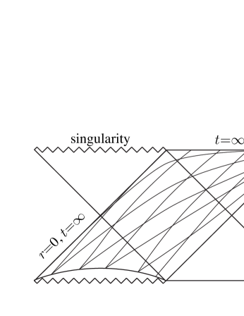
FIG. 1.: This is the Penrose diagram of the Schwarzschild-de Sitter space-times. The $K_{\mu\nu}=Hq_{\mu\nu}$ slice foliates a part of the whole space-times. $t=const.$ and $r=const.$ lines are drawn schematically.

REFERENCES

- [1] E. Witten, hep-th/0106109; M. Li, hep-th/0106184; D. Klemm, hep-th/0106247; V. Balasubramanian, P. Horava and D. Minic, JHEP 0105, 043 (2001); A. Chamblin and N. D. Lambert, Phys. Lett. B508, 369 (2001); hep-th/0107031; Y. Gao, hep-th/0107067; J. Bros, H. Epstein and U. Moschella, hep-th/0107091; S. Nojiri and S. D. Odintsov, hep-th/0107134; E. Halyo, hep-th/0107169; I. Sachs and S. N. Solodukhin, hep-th/0107173; A. J. Tolley and N. Turok, hep-th/0108119.
- [2] G. W. Gibbons and S. W. Hawking, Phys. Rev. D15, 2738 (1977).
- [3] A. Strominger and C. Vafa, Phys. Lett. B379, 99 (1996).
- [4] S. Perlmutter et al, Astrophys. J. 517, 565 (1999).
- [5] A. Strominger, hep-th/0106113.
- [6] J. Maldacena, Adv. Theor. Math. Phys., 2, 231 (1998); O. Aharony, S. S. Gubser, J. Maldacena, H. Ooguri and Y. Oz, Phys. Rep. 323, 183 (2000).
- [7] S. Nojiri and S. D. Odintsov, hep-th/0106191.
- [8] L. Randall and R. Sundrum, Phys. Rev. Lett. 83, 3370 (1999); 4690 (1999).
- [9] J. de Boer, E. Verlinde and H. Verlinde, JHEP 0008, 003 (2000).
- [10] T. Shiromizu and D. Ida, Phys. Rev. D64, 044015 (2001).
- [11] A. Ashtekar and S. Das, hep-th/9911230.
- [12] S. W. Hawking and I. Moss, Phys. Lett. 110B, 35 (1982).
- [13] K. Nakao, T. Shiromizu and K. Maeda, Class. Quantum Grav. 11, 2059 (1994).
- [14] L. F. Abbott and S. Deser, Nucl. Phys. B195, 76 (1982).
- [15] T. Shiromizu, K. Nakao, H. Kodama and K. Maeda, Phys. Rev. D47, 3099 (1993).
- [16] R. Arnowitt, S. Deser and C.W. Misner, in Gravitation, an Introduction to Current Research, edited by L. Witten (Wiley, New York, 1962).
- [17] R. Bartnik, Commun. Math. Phys. 94, 155 (1984); R. Bartnik, P. T. Chrusciel and N. O. Murchadha, Commun. Math. Phys. 130, 95 (1990).
- [18] K. Nakao, K. Maeda, T. Nakamura and K. Oohara, Phys. Rev. D44, 1326 (1991).
- [19] G. C. MacVittie, Month. Not. Roy. Astron. Soc. 93, 325 (1933); M. Kihara and H. Nariai, Prog. Theor. Phys. 65, 1613 (1981).
- [20] T. Shiromizu, Phys. Rev. D49, 5026 (1994); D. Kastor and J. Traschen, Class. Quantum Grav. 13, 2753 (1996); T. Shiromizu, Phys. Rev. D60, 064019 (1999).
- [21] A. Ashtekar and R. O. Hansen, J. Math. Phys. 19, 1542 (1978); A. Ashtekar and A. Magnon, J. Math. Phys. 25, 2682 (1984).
- [22] A. Komar, Phys. Rev. 113, 934 (1959).
- [23] V. Balasubramanian and P. Kraus, Commun. Math. Phys. 208, 413 (1999).
- [24] J. D. Brown and J. W. York, Phys. Rev. D47, 1407 (1993).
- [25] S. B. Gidding, E. Katz and L. Randall, JHEP 0003, 023 (2000).
- [26] O. Henkel, gr-qc/0108003.