Density Perturbations in the Ekpyrotic Scenario

Abstract

We study the generation of density perturbations in the ekpyrotic scenario for the early universe, including gravitational backreaction. We expose interesting subtleties that apply to both inflationary and ekpyrotic models. Our analysis includes a detailed proposal of how the perturbations generated in a contracting phase may be matched across a ‘bounce’ to those in an expanding hot big bang phase. For the physical conditions relevant to the ekpyrotic scenario, we re-obtain our earlier result of a nearly scale-invariant spectrum of energy density perturbations. We find that the perturbation amplitude is typically small, as desired to match observation.

We recently proposed a novel scenario for the early Universe in which the hot big bang is created by the collision between two M-theory branes[1]. The scenario assumes the Universe begins in an almost static, nearly BPS initial state consisting of empty, flat, parallel three-branes. In the effective 4d theory, the BPS state is homogeneous and has zero spatial curvature. Due to non-perturbative effects, however, a tiny force attracts the branes to one another. As the branes come together, quantum fluctuations create ripples in the brane surfaces that result in spatial variations in the time of collision. Consequently, some regions heat up and begin to cool before others, producing a spectrum of long wavelength density perturbations which can seed structure formation in the Universe.

We estimated the perturbation spectrum using a ‘time delay’ formalism[2], often used in simplified treatments of inflationary models. In that context, spatial variations in the time when inflation ends result in long wavelength density inhomogeneities. We applied the same formalism to variations in the time of collision in the ekpyrotic scenario. The equation for fluctuations in the scalar field $\phi$ describing the inter-brane separation in the ekpyrotic model is almost identical to that describing fluctuations in the inflaton during slow-roll inflation. Consequently, a nearly scale-invariant spectrum of fluctuations is found. The result is remarkable because it shows that the Harrison-Zel’dovich spectrum can be obtained without inflation in a space-time which is very nearly static Minkowski space.

The time delay formalism is a crude approximation, and only quantitatively accurate for a small class of inflationary potentials [3]. Nevertheless, it often gives a good estimate of the spectral index for the power spectrum of perturbations. One of the goals of this paper is to investigate whether the same statement is true for the ekpyrotic model.

In the case of the ekpyrotic model, there is the major complication that the perturbations are produced when the effective 4d scale factor is contracting. In order to have a viable scenario, a mechanism must be found to reverse from contraction to expansion. This issue has been addressed in a recent paper we have written with N. Seiberg[4], where we argue that such a ‘bounce’ may be allowed in the context of M-theory, where it corresponds to a collision and rebound of the outer boundary branes. A matching rule linking the homogeneous background variables of the contracting phase to those describing the expanding phase was suggested there. Assuming this proposal is valid, what remains is to apply and extend those ideas to describe the evolution of perturbations through the moment of reversal.

A stimulus for the present work was a paper by D. Lyth[5], which calculated the growth of the perturbation variable $\zeta$ (also commonly termed ${\cal R}$) representing the curvature perturbation of spatial slices which are comoving with the matter. Lyth correctly showed that $\zeta$ was not amplified in the contracting phase of the ekpyrotic universe. He claimed this implied that when gravitational back-reaction was included, the spectrum of density perturbations became strongly scale-dependent with negligible power on large scales, making the ekpyrotic scenario incompatible with observations. His analysis employed a certain class of analytically solvable models with exponential potentials, previously used to describe power law inflation[6] and simply extended to the situation of slow contraction relevant to the ekpyrotic scenario. We repeat his analysis here, but also compute the perturbation in the Newtonian potential $\Phi$. We show that in the contracting phase gravitational back-reaction actually enhances rather than suppresses long wavelength fluctuations, but these fluctuations show up purely in $\Phi$ and not in $\zeta$. Therefore gravitational back-reaction does not spoil the ekpyrotic mechanism, at least in the contracting phase.

The remaining issue regards the appropriate matching condition for tracking the perturbations across the bounce and into the expanding hot big bang. Consistent with the arguments of Ref. 4, we seek to identify variables which are non-singular at the bounce, both for the background and perturbation variables. We then match the amplitudes of the two linearly independent solutions for the perturbation variables across the bounce. With our prescription, we find that the long wavelength perturbations developed in the contracting phase do indeed survive to the expanding phase, provided there is a change in the equation of state at the bounce, such as occurs if a sub-dominant component of radiation is produced there. Our final expression for the density perturbation spectrum agrees well with the more naive time delay estimate.

After communicating a preliminary version of this paper to Lyth and R. Brandenberger, Lyth prepared a second manuscript[7] proposing that contraction be matched to expansion on a time-slice of fixed energy density[7]. With this procedure, he argues that the curvature perturbation $\zeta$ is conserved across the bounce. But since $\zeta$ does not acquire a scale invariant spectrum in the contracting phase, he argues that $\zeta$ will not have such a spectrum in the expanding phase, where it represents the amplitude of growing mode adiabatic perturbations. Lyth’s conclusion is that any growing mode density perturbations developed in the contracting phase match perfectly onto pure decaying mode perturbations in the expanding phase. Brandenberger and Finelli[8], and Hwang[9], have recently produced preprints repeating this argument. In a note added, at the end of this paper, we explain why we do not believe these conclusions are valid for the ekpyrotic scenarios proposed in Refs. 1 and 4.

Let us outline our approach to the matching problem. We want to evolve background and perturbation variables according to the appropriate field equations, all the way to to zero scale factor in the four dimensional effective theory. We identify a complete set of variables which are non-singular at the bounce, and match those non-singular variables across it. This prescription automatically excludes the variables $\Phi$ and $\zeta$, both of which diverge. More generally, geometrical quantities such as the synchronous gauge comoving metric perturbation $h_{ij}$ also diverge. Indeed the meaning of the three-geometry is unclear at zero scale factor.

Instead our approach is essentially algebraic rather than geometrical. We focus on gauge invariant perturbation variables which are consistently small at all times and match these across the bounce at $t=0$. We argue that this matching would give consistent results for an infinite class of perturbation variables so defined. Our prescription can only be fully justified by a satisfactory microscopic description of the relevant degrees of freedom. Nevertheless, if string theory shows that the scale factor can truly pass through zero and bounce, then tracking perturbative gauge-invariant degrees of freedom which remain small and finite seems likely to be the right approach to matching fluctuations across the bounce.

Our analysis shall be performed entirely within the context of four dimensional effective field theory. This does not capture all the low energy degrees of freedom relevant to the five (or indeed eleven) dimensional brane-world. As in Ref. 1, we shall assume those other degrees of freedom are frozen, or at least so slowly varying that their inclusion would not substantially alter the result. We shall focus here on single moduli field $\phi$ which determines the outer brane separation in a brane-world Universe. In Ref. 1 we considered a model in which the perturbations are produced by the collision of a bulk brane with one of the boundary branes. As we pointed out there, if the 4d effective theory is valid, the scale factor in that theory must continue to contract until the outer branes collide and bounce. In Ref. 4 we suggested a simplified model in which there is only one collision between the boundary branes and no bulk brane is needed. The perturbations are produced as the outer branes approach one another. For simplicity, here we shall restrict ourselves to this two-brane scenario, in which the same scalar field $\phi$ is responsible both for the development of the perturbations, and for describing the the outer-brane collision and bounce. Generalizations to bulk-boundary collisions, as in the original scenario of Ref. 1, are a straightforward extension and will be briefly mentioned when appropriate.

The outline of this paper is as follows. In Section I we discuss the properties of the inter-brane potential relevant to the ekpyrotic scenario, an issue referred to again in the note added at the end of this paper. We then review the application of the time delay formalism to the ekpyrotic scenario, as described in Ref. 1, showing that a scale invariant spectrum of fluctuations is naturally predicted. In Section II, we show that including gravitational back-reaction has, in Newtonian gauge, only negligible effects on the fluctuations acquired by the scalar field. Section III is devoted to a discussion of the role of the curvature perturbation $\zeta$ (or ${\cal R}$) conventionally used in the analysis of inflationary models, which is in fact insensitive to the growing mode perturbation in the contracting phase of the ekpyrotic model. This is further elaborated in Section IV where we show that $\zeta$ is canonically conjugate to the direction of amplification, which is proportional to the variable $\Phi$. As a consequence of Liouville’s theorem, $\zeta$ is ‘squeezed’ as the perturbations develop during the collapsing phase of the ekpyrotic scenario.

Section V addresses the key moment of reversal, which is when, in the four dimensional effective description, the Universe ‘bounces’ as the scale factor $a$ hits zero. Since the four dimensional spacetime geometry is singular there, a four dimensional geometrical description using the Einstein frame metric is inappropriate. However, our approach is to identify a complete set of dynamical variables which remain finite at the bounce and to match them at the transition from contraction to expansion. We ignore divergent quantities as unphysical, attributing their bad behavior to a singular choice of field and metric variables. We used this approach in Ref. References to describe the homogeneous background evolution during the bounce. Here we shall show that there is also a set of gauge invariant linear perturbation variables which are well-behaved at the bounce. When the theory is formulated in these variables, there is a well defined matching prescription, even in the four dimensional effective field theory, which seems to yield physically sensible results.

In order for the well-behaved variables to exist, we emphasize that it is important to have two conditions: (1) there must be a free scalar field (the modulus $\phi$ in our case) whose kinetic energy diverges at the bounce and (2) the scalar potential $V(\phi)$ must be sufficiently non-singular at the bounce. The simplest case is where $V(\phi)$ approaches zero at the bounce, as suggested by the mapping from M-theory to weakly coupled string theory[4]. If these two conditions are fulfilled, then it is possible to follow the perturbations and match at $a=0$.

Our main finding, in Sections V and VI, is that as long as radiation is produced or fields are excited at the outer-brane collision so that there is a jump in the first or second time derivative of the equation of state parameter $w\equiv P/\rho$, the scale invariant perturbation spectrum developed during the contracting phase propagates through the bounce and into the final expanding Universe. Intriguingly, the final density perturbation amplitude derived in Section VI is naturally suppressed by a small numerical coefficient, by quantities which are automatically small in Horava-Witten theory, and by factors involving the efficiency with which brane kinetic energy is converted into radiation. We comment on how this suppression may naturally explain the small perturbation amplitude $\sim 10^{-5}$ we see via observations of the cosmic microwave sky in the universe today.

I Time Delay Neglecting Gravity Pre-Collision

We first derive the ekpyrotic spectrum in a very naive ‘time delay’ approach which totally neglects cosmological expansion, gravity and all moduli other than $\phi$. We also ignore the crucial element of reversal from contraction to expansion, which will be a critical aspect of the discussion in Sections V and VI. As we shall see, despite the fact that the time delay argument ignores these very important features, it nevertheless comes close to matching our final answer. Thus, as is the case in inflation, the time delay argument turns out to be a convenient heuristic even though it is neither physically rigorous nor numerically accurate.

We assume that at large positive $\phi$ the effective potential governing the evolution of $\phi$ takes the form

$$V=-V_{0}e^{-c\phi},$$ (1)

where $V_{0}$ and $c$ are positive constants. The ekpyrotic scenario starts at large positive $\phi$, in a state of nearly zero energy, and rolls towards negative values. As $\phi$ becomes increasingly negative and the branes come close together, $V(\phi)$ must turn upwards and approach zero. As discussed in Ref. References, for example, this is the behavior to be expected in M-theory because the string coupling constant vanishes as the outer branes collide. (A similar constraint applies in the bulk brane collision, as discussed in Ref. 1.)

Generally, in brane world models, the separation of the two boundary branes can be described by a canonically normalized, minimally coupled scalar field $\phi$ (the ‘radion’). As the brane separation $d$ goes to zero, one can ignore the effect of the bulk ‘warp factor’ and one obtains the Kaluza-Klein result in which $d\sim e^{\sqrt{2/3}\phi/M_{Pl}}\rightarrow 0$ as $\phi\rightarrow-\infty$. (Here and below, $M_{Pl}=(8\pi G)^{-{1\over 2}}$ is the four dimensional reduced Planck mass.) In standard Kaluza-Klein theory, the same dependence holds at large $\phi$, so the range of $\phi$ is $-\infty<\phi<\infty$. But the presence of a bulk warp factor alters this. In many models, when the outer-brane distance $d$ tends to infinity, $\phi$ tends to a finite value, which may be taken to be zero. For example, for a pair of positive and negative tension boundary branes with a bulk Anti-de Sitter space, the inter-brane distance is $d=L$ ln(coth($-\phi/\sqrt{6}M_{Pl}))$ where $L$ is the AdS radius [1]. A suitable ekpyrotic potential would then behave as $\sim-(-\phi)^{N}\sim-e^{(-Nd/L)}$, at small $\phi$, and we would be interested in starting the system in a state such that $\phi\rightarrow 0$ at large negative times. In models with a bulk brane, such as those considered in Ref. 1, the location of the bulk brane would again be described by a scalar field, but this time its range would be finite. The exponential model (1) is useful, since it is mathematically tractable. However, one should remember, in general it should only be expected to apply over some finite range of $\phi$.

We now review how the time delay formalism can be applied to our example. The classical solution is given by solving $\dot{\phi}=-\sqrt{-2V}$. For $V(\phi)$ given in (1), we obtain

$$-t=\int_{-\infty}^{\phi}{d\phi\over\sqrt{2V_{0}}}e^{c\phi/2}={2\over c\sqrt{2V_{0}}}e^{c\phi/2}=\sqrt{2\over-V_{,\phi\phi}}.$$ (2)

where the time $t$ is large and negative at large $\phi$. We follow the evolution to some finite, small negative $t$, at which point the modes of interest are ‘frozen in’. For small fluctuations, expanding in plane waves $\delta\phi\equiv\sum_{\vec{k}}e^{i\vec{k}\cdot\vec{x}}\delta\phi_{\vec{k}}(t)$, one finds

$$\delta\ddot{\phi}_{\vec{k}}=-k^{2}\delta\phi_{\vec{k}}-V_{,\phi\phi}\delta\phi_{\vec{k}}=-k^{2}\delta\phi_{\vec{k}}+{2\over t^{2}}\delta\phi_{\vec{k}}$$ (3)

(using the solution Eq. (2) above). Curiously, even though the background here is nearly static, this is the same equation as that governing a massless field $\chi$ in a de Sitter background (with $\chi=\phi/a$, with $a$ the scale factor and $t$ conformal time). As in that case, starting from an initial Minkowski vacuum one generates a long wavelength spectrum of scale invariant fluctuations.

We assume that the quantum fluctuation $\delta\phi_{\vec{k}}$ starts in the Minkowski vacuum, $\langle|\delta\phi_{\vec{k}}|^{2}\rangle\propto k^{-1}$, so the amplitude of normalized modes with wavenumber $k$ is $\sim k^{-1/2}$. Consider a mode where $-kt_{i}\gg 1$, where $t_{i}$ is the initial time. The mode oscillates at fixed amplitude $k^{-1/2}$ until $t$ increases to $t_{1}\approx-k^{-1}$, when the destabilizing $2/t^{2}$ term in (3) begins to dominate over the stabilizing $k^{2}$ term. One then has $\delta\ddot{\phi}_{\vec{k}}\sim(2/t^{2})\delta\phi_{\vec{k}}$, with growing solution $\delta\phi_{\vec{k}}\propto(-t)^{-1}$. Hence, the final amplitude for the fluctuation, as $t$ approaches zero, is $\delta\phi_{\vec{k}}\sim k^{-1/2}(-t_{1})/(-t)\sim k^{-3/2}(-t)^{-1}$. The precise result for the long wavelength spectrum is

$$\langle|\delta\phi_{\vec{k}}|^{2}\rangle={1\over 2k^{3}t^{2}},\qquad-kt<<1,$$ (4)

which is scale-invariant as claimed.

A naive estimate of the final density perturbation amplitude runs as follows. The scalar field fluctuations give rise to a time delay in the moment of collision. Neglecting gravitational effects, the time delay between collisions relative to the mean collision time is $-\delta\phi/\dot{\phi}_{0}$. The net density perturbation after collision is then just ${\delta\rho\over\rho}\sim-4H\delta t$ where $H$ is the Hubble parameter at the time of collision. Despite the deficiencies of this time delay approach, this answer is quite close to the result we shall eventually derive, including gravitational back-reaction and matching across the bounce, which we give in equation (74) below.

The first step in improving the above treatment is to include gravitational backreaction in the initial, contracting phase. For this purpose, we focus on the gravitational backreaction corrections to Eq. (4).

II Including Gravitational Backreaction

For exponential potentials, there exist analytic scaling solutions to the Friedmann-Robertson-Walker equations which at large negative $t$ approximate the assumed initial conditions in the ekpyrotic setup, and which allow an analytic treatment [6]. For the exponential potential considered as an approximation over some range of $\phi$ in the ekpyrotic scenario, one has the background solution

$$a(t)=(-t)^{p},\qquad\phi_{0}(t)={2\over c}{\rm ln}(-Mt),$$ (5)

where $a(t)$ is the scale factor, $t$ is proper FRW time, taking negative values, and

$$p={2\over c^{2}M_{Pl}^{2}},\qquad M^{2}={V_{0}\over M_{Pl}^{2}p(1-3p)},$$ (6)

and $M_{Pl}=(8\pi G)^{-{1\over 2}}$ is the reduced Planck mass. Some useful quantities are:

$$H\equiv{\dot{a}\over a}={p\over t},\qquad\dot{\phi}_{0}=\sqrt{2p}{M_{Pl}\over t},\qquad V=-p(1-3p){M_{Pl}^{2}\over t^{2}},\qquad V_{,\phi\phi}=-{2\over t^{2}}(1-3p),$$ (7)

where dot denotes $d/dt$. In ekpyrotic models, we are interested in potentials in which the evolution is very slow or, equivalently, for which $p<<1$. (Parenthetically, note that the same solution, for $p>1$, describes a universe undergoing power law inflation). The conformal time is

$$\tau=-\int_{t}^{0}{dt\over a(t)}=-{(-t)^{1-p}\over(1-p)}={t\over a(1-p)},$$ (8)

running from $-\infty$ to $0$ as $t$ does, although as mentioned we shall have to alter the form of the potential as $t$ and $\tau$ approach zero, to avoid its diverging to minus infinity. Derivatives with respect to $t$ shall, as above, be denoted by dots and henceforth, derivatives with respect to $\tau$ shall be denoted by primes.

Mathematically, Newtonian gauge is convenient for studying scalar field perturbations since the linearized equations reduce to a single second order differential equation for the Newtonian potential $\Phi$ (for a derivation see e.g. Ref. References),

$$\Phi^{\prime\prime}+2{A^{\prime}\over A}\Phi^{\prime}+k^{2}\Phi+2\phi_{0}^{\prime}\left({{\cal H}\over\phi^{\prime}_{0}}\right)^{\prime}\Phi=0,$$ (9)

where $A\equiv(\dot{\phi}_{0})^{-1}$, and ${\cal H}\equiv a^{\prime}/a$. Here, and below, the wavenumber dependence of all perturbation quantities is not shown explicitly. For $\Phi$ one should read $\Phi_{\vec{k}}$ and so on.

We now eliminate the first derivative term by setting $\Phi=u/A$, obtaining

$$u^{\prime\prime}-{A^{\prime\prime}\over A}u+k^{2}u+2\phi_{0}^{\prime}\left({H\over\dot{\phi}_{0}}\right)^{\prime}u=0.$$ (10)

Substituting the above scaling solution, we obtain

$$u^{\prime\prime}=-k^{2}u+{p\over(1-p)^{2}\tau^{2}}u,$$ (11)

which is a form of Bessel’s equation, with corresponding order $\nu={1\over 2}(1+p)/(1-p)$. Note that our notation for the variable $u$, and for the variable $v$ introduced later, matches Mukhanov’s original notation [12].

The initial conditions are that the scalar field fluctuations should be in the Minkowski vacuum state as $\tau\rightarrow-\infty$: in Newtonian gauge, two constraints determine $\Phi$ and $\dot{\Phi}$ in terms of $\delta\phi$ and $\dot{\delta\phi}$:

$$\delta\phi = {2M_{Pl}^{2}\over\dot{\phi}_{0}}\left[\dot{\Phi}+H\Phi\right],$$ (12)

$$\dot{\delta\phi} = -{2M_{Pl}^{2}\over\dot{\phi}_{0}}\left[-{\ddot{\phi}_{0}\over\dot{\phi}_{0}}\dot{\Phi}+\left\{{k^{2}\over a^{2}}+\dot{\phi}_{0}~{}\partial_{t}\left({H\over\dot{\phi}_{0}}\right)\right\}\Phi\right].$$ (13)

At large $-kt$, for $\delta\phi\sim e^{-ik\tau}/(a\sqrt{2k})$, which is the incoming Minkowski vacuum, one finds

$$\Phi\sim{i\sqrt{p}\over 2M_{Pl}k^{3\over 2}t}e^{-ik\tau}$$ (14)

which vanishes at early times, consistent with our ekpyrotic initial condition that the space is asymptotically Minkowski in the past.

Neglecting an irrelevant phase factor, the solution for $u$ is then

$$u=(-k\tau)^{1\over 2}\sqrt{{\pi\over 2}}H_{\nu}^{1}(-k\tau)\cdot{\sqrt{p}\over(2k)^{3\over 2}M_{Pl}},$$ (15)

where $H_{\nu}^{1}$ is a Hankel function and $\nu$ was given above. We follow this solution forward to conformal times at which $-k\tau<<1$, when the modes become frozen in. Converting back to $\Phi$, and using the small argument expansion for the Hankel function, again neglecting phase factors we find

$$\Phi\sim{\sqrt{p}\over 2M_{Pl}}k^{-(1+\nu)}(-\tau)^{-2\nu}(1+O(p)).$$ (16)

Since we are interested in $p<<1$, we henceforth neglect corrections of order $p$ to the numerical coefficient. But we keep the $p$ dependence in the scaling with wavelength and time for comparison with later results.

Now we can convert back to the scalar field $\delta\phi$, using the formulae (13) given above, and obtain:

$$\delta\phi={2M_{Pl}^{2}\over\dot{\phi}_{0}}\left[\dot{\Phi}+H\Phi\right]\sim 2^{-1/2}k^{-(1+\nu)}(-t)^{-(1+p)}.$$ (17)

where we used $\Phi\propto(-\tau)^{-2\nu}\propto(-t)^{-(1+p)}$. The resulting power spectrum of fluctuations is:

$$\langle|\delta\phi_{\vec{k}}|^{2}\rangle\sim\frac{1}{2}k^{-2(1+\nu)}(-t)^{-2(1+p)}=\langle|\delta\phi_{\vec{k}}|^{2}\rangle^{(0)}{1\over k^{2p/(1-p)}(-t)^{2p}},$$ (18)

where $\langle|\delta\phi_{\vec{k}}|^{2}\rangle^{(0)}$ is the result obtained in Eq. (4) ignoring gravitational backreaction. Recalling that the regime of interest for the ekpyrotic scenario is small $p$, we see that we obtain the same answer as in Eq. (4) up to small corrections. The backreaction produces a slight reddening of the power spectrum, presumably because long wavelength perturbations were generated sooner and had longer to self-gravitate. However, since in the ekpyrotic scenario we have $p<<1$, these corrections to the spectral index are actually smaller than corrections arising from the nontrivial kinetic term for $\phi$, which were computed in Ref. 1. The result shows that backreaction and metric fluctuations have an insignificant effect on the density perturbations developed during the initial, contracting phase of the ekpyrotic universe.

III The curvature perturbation in the contracting phase

Rather than solve for the evolution of the Newtonian potential in Eq. (9), a common procedure used for inflationary models is to track the curvature perturbation on spatial slices which are comoving with the matter. As we shall discuss, this variable is in fact insensitive to the growing mode density perturbation in the contracting phase.

Following the notation of Mukhanov et al. [12], we denote the curvature perturbation on comoving slices by $\zeta$, defined by

$$\zeta\equiv\frac{2}{3}\frac{{\cal H}^{-1}\Phi^{\prime}+\Phi}{1+w}+\Phi={{\cal H}\Phi^{\prime}+{\cal H}^{2}\Phi\over 4\pi G\phi_{0}^{\prime 2}}+\Phi,$$ (19)

where ${\cal H}\equiv a^{\prime}/a$ and $w$ is the ratio of pressure to density in the background universe. The variable $\zeta$ was introduced by Bardeen[11] in his classic paper, in which it was termed $\phi_{m}$. It was employed in the context of inflation by Bardeen, Steinhardt, and Turner [13] and its use later elaborated upon by many authors [12, 14, 6]. Mukhanov et al. [12] re-express $\zeta$ as $\zeta=v/z$ (for spatially flat hypersurfaces) and thereby derive the ‘$v$-equation’:

$$v^{\prime\prime}=-k^{2}v+\frac{z^{\prime\prime}}{z}v$$ (20)

where $z=a\phi_{0}^{\prime}/{\cal H}$. For the power law solution given in equation (7), this reads:

$$v^{\prime\prime}=-k^{2}v-{p(1-2p)\over(1-p)^{2}\tau^{2}}v.$$ (21)

Since the last term is negative, it follows that there is no classical instability in the variable $v$, a point emphasized by Ref. 3. (Note that Ref. 3 relabels Mukhanov’s $v$ variable as $u$; here we have kept to the original notation.)

However, this does not at all imply the absence of a growing mode density perturbation: the variable $\Phi$ does exhibit an instability, as we have discussed above. Given a solution $v$, the potential $\Phi$ can be obtained by solving

$$k^{2}\Phi=-4\pi G{\phi_{0}^{\prime 2}\over{\cal H}}(v/z)^{\prime}.$$ (22)

The general solution to the $v$-equation to order $k^{2}$ is:

$$v=C_{1}z\left(1-k^{2}\int^{\tau}_{-\infty}\frac{d\tau^{\prime}}{z^{2}}\int^{\tau^{\prime}}_{-\infty}z^{2}d\tau^{\prime\prime}\right)+C_{2}z\left(\int^{\tau}_{-\infty}\frac{d\tau^{\prime}}{z^{2}}-k^{2}\int^{\tau}_{-\infty}\frac{d\tau^{\prime}}{z^{2}}\int^{\tau^{\prime}}_{-\infty}z^{2}d\tau^{\prime\prime}\right),$$ (23)

where $C_{1}$ and $C_{2}$ are arbitrary constants. Substituting into Eq. (22), we obtain

$$\Phi=\bar{C}_{1}\Phi_{0}\int^{\tau}_{-\infty}z^{2}d\tau^{\prime}+\bar{C}_{2}\Phi_{0}$$ (24)

where $\Phi_{0}\equiv a^{\prime}/a^{3}$, and $\bar{C}_{0}$ and $\bar{C}_{2}$ are constants. For the power law solutions studied here, $z\propto a$. For an expanding universe, the first term dominates the second as $t\rightarrow\infty$. However, for a contracting universe, the second term is the proper growing mode as $t\rightarrow 0$. The solution is the same as that found in Eq. (16), from which we derived the scale-invariant spectrum.

Various subtleties are worthy of further comment. First note that $\Phi_{0}\equiv a^{\prime}/a^{3}$ is an exact solution of the perturbation equation (9) for $k=0$. In fact, for $k=0$, the perturbation $\Phi_{0}$ just represents a coordinate transformation of the the time $t$, and is therefore unphysical. However, for nonzero $k$ the solutions tending towards $\Phi_{0}$ are not gauge modes and therefore represent a real gravitational instability.

Second, note that $\zeta$ is insensitive to any component of $\Phi$ tending towards $\Phi_{0}$, as may be seen from the expression

$$\zeta=\frac{2}{3a^{2}(1+w)}\left(\frac{\Phi}{a^{\prime}/a^{3}}\right)^{\prime}.$$ (25)

For inflationary models, tracking $\zeta$, as is done in many analyses, is useful because the components that are projected out in this formula are harmless decaying modes. However, for the ekpyrotic model, the growing mode tends to $\Phi_{0}$. One can in fact recover the the growing mode solution from $\zeta$ or $v$, but special care has to be taken to do so, by keeping the next order terms in $k^{2}$ as we have done above.

IV Canonical Conjugates and ‘Squeezing’

In this section we show that the variables $u$ in Eq. (10) and $v$ in Eq. (20) at the heart of the analysis of the previous sections are in fact canonically conjugate. The importance of this is that in the $(p,q)$ phase space plane, the trajectories of the system are focused towards certain lines - for example the line $p=q$ in the case of the upside-down harmonic oscillator. These lines are then the classically amplified directions in phase space, and from Liouville’s theorem the phase space density is necessarily squeezed in the orthogonal directions. While the calculation of Reference 5 is indeed correct, it does not by itself indicate the absence of a growing mode density perturbation, because the curvature perturbation which was computed is actually orthogonal to the direction in which fluctuations are amplified in the ekpyrotic setup. (We note that References References and References agree with this conclusion).

Our starting point is the action for gravity plus a scalar field in canonical (first order) form. The relevant formulae may be found for example in Ref. References. The Newtonian potential $\Phi$ is written in terms of $u$, and $\zeta$ is written in terms of $v$ as above. One finds the quadratic action for perturbations reduces to

$${\cal S}={2M_{Pl}^{2}\over p}\int d\tau\left(vF^{\prime}+{\beta\over\tau}vF-{1\over 2}F^{2}-{k^{2}\over 2}v^{2}\right),$$ (26)

where $\beta=p/(1-p)$, $F\equiv k^{2}u$, and we have written the Laplacian $\nabla^{2}$ as $-k^{2}$. The sum over all Fourier modes is implicit.

The action (26) is in canonical form $\int pq^{\prime}-H(p,q)$, with $H$ the Hamiltonian. Therefore, up to normalization, $v$ and $F$ are canonically conjugate. The equations of motion are

$$F=-\tau^{\beta}\left({v\over\tau^{\beta}}\right)^{\prime}\qquad k^{2}v=\tau^{-\beta}\left({F\tau^{\beta}}\right)^{\prime},$$ (27)

which are just the relations above: equation (22), which expresses $\Phi$ in terms of $\zeta$ and $\zeta^{\prime}$, and equation (25), which expresses $\zeta$ in terms of $\Phi$ and $\Phi^{\prime}$. These imply the equations of motion (11) and (20) used in the previous sections.

In the inflationary case, which corresponds to $p>1$ in the above analysis, both the variable $v$ and its canonical conjugate momentum $F$ (or $u$) obey equations exhibiting a classical instability: both are amplified as $\tau$ approaches zero. The system starts near $v=u=0$, with only small quantum fluctuations. As time proceeds the system evolves away from the origin along a certain line, $u\propto v$ in phase space. By Liouville’s theorem, the phase space density is ‘squeezed’ in the direction orthogonal to this line. But in the ekpyrotic case, $p<<1$, the $v$ (or $\zeta$) variable is instead stable and classical trajectories instead run out along the $u$ (or $\Phi$) axis. The $v$ (or $\zeta$) direction must in consequence be ‘squeezed’. Thus there is no classical growth in $\zeta$, consistent with the finding of Reference References.

V Reversal and A Nonsingular Matching Condition

Having established that there is indeed a growing mode scale-invariant spectrum of density perturbations in the collapsing phase, we now turn to the more challenging question of whether these perturbations survive the reversal to expansion. We have recently addressed the issue of reversal in a paper with N. Seiberg[4], and we shall employ and extend the analysis of that paper here.

As we have discussed, the variable $\zeta$ is not amplified in the collapsing phase, since it is insensitive to the growing mode perturbation. However, $\zeta$ does yield the amplitude of the growing mode perturbation in the expanding phase. Therefore, if $\zeta$ was in fact the correct variable to match at $\tau=0$, the growing mode perturbation which developed in the collapsing phase would just match onto a pure decaying mode perturbation in the expanding phase. This has indeed been suggested by Lyth in a follow-up paper following our communication of the above calculations to him [7]. The new argument is essentially that perturbation evolution may reverse at collision. That is, $\Phi$ began negligibly small, grew to be very large at the bounce but then, after reversal to expansion, $\Phi$ shrank precisely back to zero.

In this section, we wish to explain why matching $\zeta$ across the bounce is not appropriate in the scenarios we consider. Instead, we claim, the scale invariant growing mode spectrum generated in the contracting phase matches onto a linear combination of growing and decaying modes at reversal. Consequently, the density perturbations survive the reversal of the scale factor to seed structure formation in the hot big bang.

In order to analyze matching at the bounce, gauge invariant variables must be identified which are well-behaved as $a$ and $\tau$ approach zero. We have already seen that the growing mode solution for $\Phi$ is proportional to $a^{\prime}/a^{3}$, which is divergent as $\tau$ tends to zero. Likewise, as discussed below, in the situation of interest, $\zeta$ is logarithmically divergent. Since linear perturbation theory can only be valid when the perturbation variables are small, it follows that $\zeta$ is not a good matching variable. Nevertheless, with careful treatment to exclude the logarithmic divergence, $\zeta$ shall be very useful in the analysis after $\tau=0$, just because it’s ‘long wavelength’ component is nearly constant in the expanding phase, and gives the amplitude of the growing mode linear density perturbation.

As mentioned in the introduction, the potential $V(\phi)$ in (1) cannot hold as $\phi\rightarrow-\infty$. In the main example we treat here, we instead assume $V(\phi)$ bends upward so that $V(\phi)\rightarrow 0$ as $\phi\rightarrow-\infty$. In this case, just before collision the system is completely described as a massless scalar field coupled to gravity, in a collapsing Universe. As discussed in Ref. 4, one can in this case define regular variables, in which the evolution through $a=0$ becomes well defined.

For the perturbation analysis, it is very important that, as $a\rightarrow 0$, the Universe is dominated by scalar field kinetic energy. In this situation, a good perturbation variable is the fractional energy density perturbation on spatial slices which are comoving with the matter, termed $\epsilon_{m}$ by Bardeen in his discussion of gauge invariant cosmological perturbation theory [11]. This variable (defined in his equation 3.13) is a linear combination of the energy density perturbation $\delta T^{0}_{0}$, and the velocity perturbation $T^{0}_{i}$, which is invariant under linearized coordinate transformations. It equals the energy density perturbation in any gauge in which the matter worldlines are orthogonal to the $\tau=$constant hypersurfaces, and as Bardeen emphasized it is the natural choice of perturbation amplitude from the point of view of the matter.

The equations of motion for the matter, $T^{\mu}_{\nu;\mu}=0$, lead to the following equations of motion,

$$(\rho a^{3}\epsilon_{m})^{\prime} = -(\rho+p)a^{3}kv_{s}^{(0)}$$ (28)

$${v_{s}^{(0)}}^{\prime}+{\cal H}v_{s}^{(0)} = k\Phi+{k\over(1+w)}(c_{s}^{2}\epsilon_{m}+w\eta),$$ (29)

where $v_{s}^{(0)}$ is the gauge-invariant velocity perturbation defined by Bardeen. Here we introduce $w=p/\rho$ parameterizing the equation of state for pressure $p$ and energy density $\rho$, $c_{s}^{2}=dp/d\rho$ being the sound speed, and $\eta$ being the ‘entropy perturbation’, defined as the difference between the pressure perturbation and that expected from the density perturbation and the background pressure-density relation. In most of the analysis below we shall assume $\eta$ is zero, which is to say that the density perturbations are ‘adiabatic’. For the types of matter we consider (perfect fluids and scalar fields), the anisotropic stress is zero, and Bardeen’s potentials are related to our potential $\Phi$ by $\Phi=\Phi_{A}=-\Phi_{H}$. With these simplifications, and for the flat universe we consider, equations (4.5) and (4.8) of Bardeen’s paper[11] reduce to (29) above.

Remarkably, scalar field kinetic energy domination implies that $\epsilon_{m}$ is actually finite at $\tau=0$. This can be seen from the Einstein constraint equation, which reads

$$\nabla^{2}\Phi=4\pi G\rho a^{2}\epsilon_{m},$$ (30)

where $\rho$ is the total background energy density. For scalar field kinetic domination, $\rho\propto a^{-6}$ as $a$ tends to zero. But the growing mode perturbation $\Phi\propto a^{\prime}/a^{3}\propto a^{-4}$ and, from Eq. (30), $\epsilon_{m}$ is finite as $a$ tends to zero.

Having identified a non-singular matching variable, we still need to decide which time slice to match on. In the present situation, this is unambiguously defined as time slice where $\phi$ tends to $-\infty$, or, re-phrased in terms of the brane separation, the time when $d\propto e^{\sqrt{2/3}\phi/M_{Pl}}\rightarrow 0$. If we assume that no radiation is present in the contracting phase, so that the only energy density present is that in $\phi$, then the surfaces of constant $\phi$ are also the comoving surfaces (because the perturbation to the momentum is proportional to $\delta\phi$), and $\epsilon_{m}$ is the fractional energy density perturbation evaluated upon these surfaces.

At the bounce, we assume that there is a change in the internal state of the branes so that $V(\phi)$ switches off and the boundary branes no longer attract. After the bounce, $\phi$ is therefore a massless, free field. We also assume some radiation is produced on the branes. Again the matching surface is defined in terms of $\phi$, but with radiation present it is not obvious that the surfaces of constant $\phi$ are still comoving with the matter. However this is indeed the case for adiabatic perturbations as the following calculation reveals.

We perform the calculation in conformal Newtonian gauge. The equation governing the evolution of the radiation perturbation is given in this gauge by

$$(\delta_{r}-4\Phi)^{\prime}={4\over 3}kv_{r},$$ (31)

where $\delta_{r}$ is the fractional energy density perturbation in the radiation and $v_{r}$ the velocity perturbation. We now make the assumption of adiabaticity, equivalent to the statement that the ratio of radiation to scalar field energy density is spatially uniform being determined locally by the microphysics of brane collision. The condition for the ‘entropy perturbation’ $\eta$, defined above, to be zero at early times is that $\delta_{r}={2\over 3}\delta_{\phi}$, where $\delta_{\phi}$ is the fractional density perturbation in the scalar field. In Newtonian gauge we have

$$\delta_{\phi}=2\left({\delta\phi^{\prime}\over\phi_{0}^{\prime}}-\Phi\right).$$ (32)

The final ingredient in calculating $v_{r}$ is the equation for perturbations in the massless scalar field,

$$\delta\phi^{\prime\prime}+2{\cal H}\delta\phi^{\prime}=4\phi_{0}^{\prime}\Phi^{\prime}-k^{2}\delta\phi.$$ (33)

¿From the adiabaticity condition and equations (31), (32) and (33), as well as the background equation $\phi_{0}^{\prime\prime}+2{\cal H}\phi_{0}^{\prime}=0$, one determines

$$v_{r}=-k{\delta\phi\over\phi_{0}^{\prime}}.$$ (34)

This is the velocity of the radiation in Newtonian gauge. We wish to transform to the time-orthogonal gauge in which $\delta\phi$ is zero. The transformation required is a shift in conformal time by $T=-\delta\phi/\phi_{0}^{\prime}$ accompanied by a shift in spatial coordinates with a potential $L$ such that $L^{\prime}=-kT$, to ensure the absence of time-space components of the metric (in the notation of Section III in Bardeen’s paper[11]). The result of these transformations is that in the $\delta\phi=0$ gauge, the velocity potential for the radiation equals $v_{r}+L^{\prime}$, which is zero. Therefore, for adiabatic initial conditions, the radiation fluid is actually comoving with the massless scalar field. Therefore the comoving slices correspond to constant scalar field slices, both before and after the bounce.

So we may therefore focus on the evolution of the energy density perturbation on comoving slices, $\epsilon_{m}$, and attempt to match it across the bounce at $\tau=0$. The equation of motion for $\epsilon_{m}$ is straightforwardly derived from (29) by eliminating $v_{s}^{(0)}$, to obtain

$$\epsilon_{m}^{\prime\prime}+f(\tau)\epsilon_{m}^{\prime}+g(\tau)\epsilon_{m}=-k^{2}w\eta,$$ (35)

where

$$f(\tau)={\cal H}(1+3c_{s}^{2}-6w),$$ (36)

$$g(\tau)={\cal H}^{2}(9c_{s}^{2}+{9\over 2}w^{2}-12w-{3\over 2})+k^{2}c_{s}^{2}.$$ (37)

As an aside, we now infer the behavior of the variable $\zeta$ at small $\tau$. One has

$$\zeta=-{(a^{2}{\cal H}\epsilon_{m})^{\prime}\over(1+w)k^{2}a^{2}}.$$ (38)

Employing the background relations

$${\cal H}^{\prime}=-{1\over 2}(1+3w){\cal H}^{2},\qquad w^{\prime}=-3{\cal H}(c_{s}^{2}-w)(1+w),$$ (39)

one obtains

$$\zeta^{\prime}={{\cal H}c_{s}^{2}\epsilon_{m}\over 1+w}.$$ (40)

Since $\zeta^{\prime}$ is down by $k^{2}$ relative to $\zeta$, the rate of change of $\zeta$ is typically much smaller than ${\cal H}\zeta$ for the low $k$ modes of interest. So one might imagine $\zeta$ would be a good matching variable. However, as noted above, $\epsilon_{m}$ is finite as $\tau$ tends to zero. From Eq. (40) and the fact that ${\cal H}\propto\tau^{-1}$ for small $\tau$, one observes that $\zeta$ diverges logarithmically at small $\tau$. Hence, as stated above, in linear perturbation theory $\zeta$ is not a good variable for establishing a matching condition at $\tau=0$. Nevertheless, $\zeta$ does have some utility. If one separates out the short wavelength piece which is divergent, the remaining long wavelength component of $\zeta$ is finite and nearly constant. This finite piece is then very useful, since it gives the amplitude of the final growing mode linear density perturbation in the expanding Universe.

We now turn to an analysis of Eq. (35). The first thing to note is that in the setup considered here, ${\cal H}$, $w$ and $c_{s}^{2}$ all have expansions in terms of simple powers of $\tau$, for either $\tau<0$ or $\tau>0$:

$${\cal H}={1\over 2}\tau^{-1}+h_{0}+h_{1}\tau+\dots,$$ (41)

$$w=1+w_{1}\tau+w_{2}\tau^{2}+\dots,$$ (42)

$$c_{s}^{2}=1+c_{1}\tau+c_{2}\tau^{2}+\dots.$$ (43)

This follows from computing

$${\cal H} = {1\over 2}{{a^{2}}^{\prime}\over a^{2}},$$ (44)

$$w = {{1\over 2}\phi^{\prime 2}-a^{2}V\over{1\over 2}\phi^{\prime 2}+a^{2}V}={3M_{Pl}^{2}Q^{2}-a^{2}U\over 3M_{Pl}^{2}Q^{2}+a^{2}U},$$ (45)

$$c_{s}^{2} = 1+{2\over 3}{V_{,\phi}a^{5}\over a^{\prime}\phi^{\prime}a^{2}}=1+{2\over 3}{a_{1}U_{,0}+a_{0}U_{,1}\over{\cal H}M_{Pl}Q},$$ (46)

where $a^{2}={1\over 4}(a_{0}^{2}-a_{1}^{2})$, $U=Va^{4}$ and $Q\equiv{1\over 4}(a_{0}a_{1}^{\prime}-a_{1}a_{0}^{\prime})$. As discussed in Ref. 4, the variables $a_{0}=2a\,{\rm cosh}(\phi/\sqrt{6}M_{Pl})$, and $a_{1}=-2a\,{\rm sinh}(\phi/\sqrt{6}M_{Pl})$ are both finite at $\tau=0$. These variables were introduced in Ref. References, with motivation from the five dimensional geometry. In the AdS case, $a_{0}$ and $a_{1}$ are the scale factors on the positive and negative tension boundary branes respectively. Although the four dimensional Einstein frame scale factor $a$ tends to zero at an outer-boundary collision, $\phi$ tends to minus infinity in just such a manner as to leave $a_{0}$ and $a_{1}$ finite at collision.

The physics of bounce and reversal are discussed in Ref. References, the results of which are assumed here. The key point for our analysis is that the equations of motion for $a_{0}$ and $a_{1}$,

$${3\over 2}M_{Pl}^{2}a_{0}^{\prime\prime}={\partial U\over\partial a_{0}}\qquad{3\over 2}M_{Pl}^{2}a_{1}^{\prime\prime}=-{\partial U\over\partial a_{1}},$$ (47)

are actually regular at $\tau=0$. It follows that all the variables in Eq. (46) have simple power series expansions around $\tau=0$, as shown in Eq. (43), for either positive or negative $\tau$.

It will be important below to include a component of radiation after the bounce. As discussed in Ref. References, the density and temperature of radiation on the branes is actually finite at $a=0$, as long as the radiation couples to the scale factors $a_{0}$ or $a_{1}$, which are both finite (and equal) as $\phi\rightarrow-\infty$. If, for example, $U$ is zero after the collision but there is a density $\bar{\rho}_{r}$ of radiation produced on the brane with scale factor $\bar{a}$ (in the simplest models, we have $\bar{a}=a_{0}$ or $a_{1}$ for the positive or negative tension branes respectively). Then the expression for $w$ in Eq. (46) is replaced by

$$w = {3M_{Pl}^{2}Q^{2}+{1\over 3}(\bar{\rho}_{r}\bar{a}^{4})a^{2}\over 3M_{Pl}^{2}Q^{2}+(\bar{\rho}_{r}\bar{a}^{4})a^{2}}.$$ (48)

Before proceeding to analyze Eq. (35), it is important to recognize that the expansion coefficients in Eq. (43) are not independent, but are related by Eq. (39). These imply, for example, that $h_{0}=-{3\over 16}w_{1}$ and $c_{1}={2\over 3}w_{1}$. The coefficient functions in Eq. (35) have the following expansions

$$f(\tau)=-{1\over\tau}+f_{0}+f_{1}\tau+\dots,\qquad g(\tau)=g_{-1}\tau^{-1}+g_{0}+g_{1}\tau+\dots,$$ (49)

with $f_{0}=-{13\over 8}w_{1}$, $g_{-1}={3\over 4}w_{1}$, and $g_{0}={21\over 32}w_{1}^{2}+k^{2}$. Now the general solution of the perturbation equation (Eq. (35)) is a sum of the two linearly independent solutions

$$\epsilon_{m} = \epsilon_{0}D(\tau)+\epsilon_{2}E(\tau),$$ (50)

where $\epsilon_{0}$ and $\epsilon_{2}$ are arbitrary constants, and

$$D(\tau) = 1+d_{1}\tau+\hat{d}_{2}\tau^{2}{\rm ln}|\tau|+\hat{d}_{3}\tau^{3}{\rm ln}|\tau|+d_{3}\tau^{3}+\dots,$$ (51)

$$E(\tau) = \tau^{2}+e_{3}\tau^{3}+\dots,$$ (52)

The equation of motion determines all the coefficients $d_{n}$, $n=1,3,4,\dots$, $\hat{d}_{n}$, $n=2,3,\dots$ and $e_{n}$, $n=3,4,\dots$. One finds $d_{1}=g_{-1}={3\over 4}w_{1}$, $\hat{d}_{2}=-{1\over 2}(d_{1}(f_{0}+g_{-1})+g_{0})=-{1\over 2}k^{2}$, and so on. Since the coefficients $w_{1}$, $w_{2}$, $\dots$ change across $\tau=0$, the two series expansions are different for $\tau<0$ and $\tau>0$. We denote the coefficients in (50), for $\tau<0$ and $\tau>0$ respectively, as $\epsilon_{0}(0^{-})$, $\epsilon_{2}(0^{-})$, and $\epsilon_{0}(0^{+})$, $\epsilon_{2}(0^{+})$. The matching rule we seek should determine the latter two constants in terms of the former.

It seems clear that we should match the amplitude of the finite perturbation variable $\epsilon_{m}$ across $\tau=0$, and this fixes $\epsilon_{0}(0^{+})=\epsilon_{0}(0^{-})$. But how should we determine $\epsilon_{2}(0^{+})$? The simplest prescription is just to set $\epsilon_{2}(0^{+})=\epsilon_{2}(0^{-})$. This amounts to matching the amplitude of the linearly independent solution which vanishes at $\tau=0$, as well as that which is finite at $\tau=0$. This prescription is invariant under redefining the independent solutions, e.g. by adding an arbitrary amount of the solution $E(\tau)$ to $D(\tau)$. Matching any other non-singular perturbation variable, defined to be an arbitrary linear combination of $\epsilon_{m}$ and $\epsilon_{m}^{\prime}$ with coefficients which are non-singular background variables (defined to possess power series expansions in $\tau$, as above) will, with the same prescription of matching the amplitudes of both linearly independent solutions, also yield precisely the same result.

This prescription is simple, but it is certainly not unique, and we emphasize that a proper understanding of the correct matching condition must ultimately rest on a better understanding of the singularity, either directly from string or M theory or from a well defined regularization and renormalization procedure.

Note that any such matching rule applied at $\tau=0$ cannot match both $\epsilon_{m}$ and $\epsilon_{m}^{\prime}$, as would be appropriate at a regular point of the differential equation. This is because $\epsilon_{m}$ and $\epsilon_{m}^{\prime}$ cannot be independently specified at $\tau=0$, just because $\tau=0$ is a singular point of the differential equation. The value of $\epsilon_{2}$ is fixed by the limit as $\tau$ tends to zero of ${1\over 2}(\epsilon_{m}(\tau)-\epsilon_{0}D(\tau))^{\prime\prime}$, so one needs to know $\epsilon_{m}^{\prime\prime}$ as $\tau$ tends to zero, in order to determine $\epsilon_{2}$.

Recall that since $\zeta$ diverges logarithmically as $\tau\rightarrow 0$, it is not a good matching variable. However, this divergence only affects the short wavelength part of $\zeta$, and the long wavelength part is still very useful since it yields the amplitude of the growing mode perturbations in the expanding phase. As we now see, the above prescription for matching $\epsilon_{m}$ actually implies that the long wavelength part of $\zeta$ has a jump across $\tau=0$. Using Eq. (39), we re-express Eq. (38) as

$$\zeta=-{{\cal H}\over(1+w)k^{2}}\left(\epsilon_{m}^{\prime}+{3\over 2}{\cal H}(1-w)\epsilon_{m}\right).$$ (53)

Substituting the above expansions, one finds the leading order behavior

$$\zeta\sim{\epsilon_{0}\over 4}({\rm ln}|\tau|-{1\over 2})+k^{-2}({1\over 2}\epsilon_{2}-{3\over 16}\epsilon_{0}w^{(2)}),$$ (54)

where $w^{(2)}\equiv w_{2}+{3\over 8}w_{1}^{2}$, plus terms which vanish as $\tau$ tends to zero. The first term is logarithmically divergent at $\tau=0$. However, since it is down by a factor of $k^{2}$, it rapidly becomes irrelevant as $\tau$ increases away from zero. The second term, the long wavelength piece $\zeta^{lw}$, is the quantity we are actually interested in. This constant, long wavelength piece is accurately conserved after the bounce as long as the matter evolution remains adiabatic, and yields the amplitude of the growing mode adiabatic density perturbation in the late Universe.

As we have discussed above, $\epsilon_{m}$ is finite at $\tau=0$ and from Section III and IV, there is no long wavelength contribution to $\zeta$ in the collapsing phase. It follows that $\epsilon_{2}={3\over 8}\epsilon_{0}w^{(2)}$ in that phase. One situation of sepcial interest is where $w^{(2)}=0$ in the collapsing phase, where the potential is irrelevant at $\phi\rightarrow-\infty$ and there is no radiation in the incoming state. In this case, $\epsilon_{2}(0^{-})=0$. In this case, we would obtain the same final result from any matching rule which set $\epsilon_{2}(0^{+})=A\epsilon_{2}(0^{-})$, with any constant $A$.

The key point is that generically $w^{(2)}$ jumps across $\tau=0$, since the background equation of state changes at the brane collision. Matching $\epsilon_{0}$ and $\epsilon_{2}$ we obtain a long wavelength contribution to $\zeta$ in the expanding phase,

$$\zeta^{lw}(\tau>0)\sim-{3\over 16}k^{-2}\epsilon_{0}(w^{(2)<}-w^{(2)>}),$$ (55)

where $w^{(2)<}$ and $w^{(2)>}$ are the values of $w^{(2)}$ for $\tau<0$ and $\tau>0$ respectively. Since $\epsilon_{m}\propto k^{2}\Phi$ and, as discussed earlier, $\Phi$ has a nearly scale invariant power spectrum, it follows from Eq. (55) that if $w^{(2)}$ undergoes a jump, then $\zeta$ will inherit a scale invariant long wavelength piece. This is our main result. In the following sections we will study a simple example of a situation where $w^{(2)}$ is discontinuous.

We shall need explicit formulae for the jump in $w^{(2)}$, and for $\epsilon_{0}$. The formulae for $w^{(2)}$ are obtained from Eqs. (46) and (48) above. If we assume that prior to $\tau=0$ there is no radiation, so that in addition to scalar kinetic energy we have only the potential $U$, then taking the limit as $\tau$ tends to zero from below one finds that

$$w^{(2)<}={2U_{0}^{2}+{4\over 3}M_{Pl}^{2}QU_{1}\over M_{Pl}^{4}Q^{2}},\qquad U_{1}=U^{\prime}|_{0}=a_{0}^{\prime}{\partial U\over\partial a_{0}}+a_{1}^{\prime}{\partial U\over\partial a_{1}},$$ (56)

where $Q={1\over 4}(a_{0}a_{1}^{\prime}-a_{1}a_{0}^{\prime})$. Likewise, for the expanding phase, if we assume $U=0$ but radiation is now present, we obtain

$$w^{(2)>}={8\over 27}{(\bar{\rho_{r}}\bar{a}^{4})^{2}\over M_{Pl}^{4}Q^{2}}.$$ (57)

Since in general $w^{(2)<}\neq w^{(2)>}$, we infer that generically, a scale invariant spectrum of perturbations will, with our prescription above, propagate across $\tau=0$ into the expanding hot big bang phase.

Finally, to compute the perturbation amplitude given in Eq. (55) we need $\epsilon_{0}$. This can be read off from the expression Eq. (16) above, by translating the $\tau$ dependence into $a^{\prime}/a^{3}$ and employing the fact that the latter gives the exact dependence for the long wavelength modes of interest even when the potential breaks away from the pure exponential form used in the first half of this paper. We find that at $\tau=0$,

$$\epsilon_{0}={4k^{1-\nu}\over 3M_{Pl}\sqrt{p}a_{0}(a_{0}^{\prime}-a_{1}^{\prime})}.$$ (58)

To summarize the results of this section, we have elaborated the conditions under which a scale invariant spectrum of perturbations survives the passage through $a=0$. Basically this requires that the equation of state, as parametrized by $w(\tau)$, have a discontinuous first or second derivative with respect to $\tau$ at $\tau=0$. This condition would appear to be quite generically fulfilled, in any situation where entropy is generated at a brane collision. A key assumption in the calculation was that the energy density is dominated by scalar field kinetic energy as we approach $a=0$. This assumption is natural in the ekpyrotic scenario, where the scalar field represents the separation of the boundary branes. We shall explore one particular, simplified model in the next section.

VI Background Evolution in a Nearly Light-like Bounce

In this section we review and extend the description of reversal from contraction to expansion, as elaborated in Reference 4. As discussed there, the background evolution is described by the variables $a_{0}$ and $a_{1}$, which for the simplest brane model (i.e. branes in AdS) represent the scale factors on the positive and negative tension boundary branes. The four dimensional effective scale factor $a$ is given by ${1\over 2}\sqrt{a_{0}^{2}-a_{1}^{2}}$, and this vanishes at the bounce.

If the potential $V(\phi)$ vanishes as $\phi$ runs off to $-\infty$ (more precisely, if the quantity $a^{4}V(\phi)$ vanishes), then the Friedmann constraint equation implies that trajectory in the $(a_{0},a_{1})$-plane intersects the boundary of moduli space $a_{0}=a_{1}$ along a light-like direction [4]. Then, if no radiation is produced on the branes, the trajectory simply reverses, corresponding to the matching condition ${a}_{0,1}^{\prime}({\rm out})=-{a}_{0,1}^{\prime}({\rm in})$. We describe this as an elastic collision, since the internal states of the two branes are unchanged by the collision.

However, at any finite velocity, the boundary brane collision must result in the production of radiation on the branes, since it is a non-adiabatic process. In the M theory context the corresponding string theory is weakly coupled near the collision, and this production of radiation should be computable once the correct matching conditions are understood.

Let us consider the case where the incoming state has no radiation, and the potential $V(\phi)$ vanishes at $t=0$ and thereafter. This requires that the potential is turned off at collision, requiring a sudden and permanent change in the internal state of the branes. Associated with this change, we assume that a small amount of radiation, with density $\bar{\rho_{r}}$ is generated, on a brane with scale factor $\bar{a}$. The collision is therefore inelastic. We parameterize the inelasticity as follows. The Friedmann constraint after collision reads

$${a}_{0}^{\prime}({\rm out})^{2}-{a}_{1}^{\prime}({\rm out})^{2}={4(\bar{\rho_{r}}\bar{a}^{4})\over 3M_{Pl}^{2}}.$$ (59)

Since right hand side is positive, the outgoing trajectory must be time-like in the $(a_{0},a_{1})$-plane. Since radiation redshifts as $\bar{a}^{-4}$, the expression $(\bar{\rho_{r}}\bar{a}^{4})$ is a constant. If radiation is generated on both branes, this term can be taken to represent the sum of the corresponding terms for both branes.

We then define the the efficiency $\xi$ with which radiation is produced by

$$\xi\equiv\frac{4(\bar{\rho_{r}}\bar{a}^{4})}{3M_{Pl}^{2}\,{{a}_{1}^{\prime}({\rm in})}^{2}},$$ (60)

which with (59) yields a single equation for the two velocities ${a}_{0}^{\prime}({\rm out})$ and ${a}_{1}^{\prime}({\rm out})$. We need another equation to fix both.

In the special case of dimensional reduction from five to four dimensions, there is a natural candidate for an approximately conserved quantity, analogous to the total momentum for an inelastic particle collision. As mentioned above, at small brane separations one has the standard Kaluza-Klein result that the size of the extra dimension is proportional to $e^{\sqrt{2/3}\phi/M_{Pl}}$. As stated above, we are assuming that the potential $V(\phi)$ vanishes as $\phi$ tends to $-\infty$. Other terms in the Lagrangian describing matter on the branes may in principle acquire $\phi$-dependence upon dimensional reduction. However, the terms describing massless gauge fields and fermions do not obtain any such $\phi$-dependence due to their conformal invariance in four dimensions. (To see this, note that the four dimensional Einstein-frame metric $g_{\mu\nu}$ is conformally related to the four dimensional components of the five dimensional metric.) Therefore at the classical level, in the $\phi\rightarrow-\infty$ limit, the Lagrangian describing gravity, $\phi$ and four dimensional radiation possesses a global symmetry $\phi\rightarrow\phi\,+\,{\rm constant}$, and it is plausible that the corresponding Noether charge $Q$,

$$Q\equiv{1\over 4}(a_{0}{a}_{1}^{\prime}-a_{1}{a}_{0}^{\prime})\propto a^{2}{\phi^{\prime}},$$ (61)

tends to a constant as the collision approaches. In this limit the classical equation of motion of $\phi$ is just $Q^{\prime}=0$.

However, the sign of $Q$ must flip at the bounce. As argued in Ref. 4, this is essential in order that the trajectory remains in the physical region of the $(a_{0},a_{1})$-plane. The reversal of $Q$ may be also understood by the following higher-dimensional argument. The value of $Q$ at collision is proportional to the time derivative of log$(a_{0}/a_{1})$. The latter quantity is the distance, rather than the vector displacement, between the boundary branes. Hence, if the branes come together and then draw apart, $Q$ must change sign although its magnitude remains constant. It is therefore natural to impose the $Z_{2}$ symmetry at $t=0$, $Q\rightarrow-Q$, which should become exact in the limit that the collision velocity approaches zero.

These arguments suggest that we parameterize $Q$-violation at the bounce (brane collision) using

$$\Delta\equiv{Q({\rm out})+Q({\rm in})\over Q({\rm in})},$$ (62)

where $\Delta$ is expected to be small. Equations (59), (60) and (62) together uniquely parameterize the final values of $a_{0}^{\prime}$ and $a_{1}^{\prime}$ after the bounce:

$${a}_{0}^{\prime}({\rm out}) = \left(1-\Delta+{\xi\over 4(1-\Delta)}\right){a}_{1}^{\prime}({\rm in})$$ (63)

$${a}_{1}^{\prime}({\rm out}) = -\left(1-\Delta-{\xi\over 4(1-\Delta)}\right){a}_{1}^{\prime}({\rm in}).$$ (64)

An example of an ekpyrotic two-brane collision is shown in Figure 1, for a specific choice of the inter-brane potential. Both branes initially expand under the influence of the attractive potential. But when they get close, and the potential rises to zero, this decelerates $a_{0}$ so that it begins to contract. At collision, $a_{0}^{\prime}({\rm in})=-a_{1}^{\prime}({\rm in})$. Immediately afterwards, $a_{0}^{\prime}$ is positive and, for small $\xi$, $a_{1}^{\prime}$ is negative.

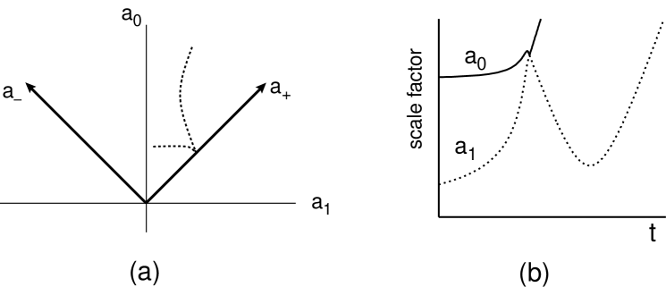
Figure 1: Sketch of a nearly light-like collision between two boundary branes. The potential employed was $a^{4}V(\phi)=-a_{1}^{4}(a_{1}/a_{0})^{4}e^{-f}$ where $f={1\over 10}\left((a_{0}/a_{1})-1\right)^{-1}$, chosen so that when expressed in terms of $\phi$, the potential $V$ vanishes as $\phi\rightarrow-\infty$, in a manner mimicking the vanishing of a non-perturbative potential $V\propto e^{-{1\over g^{2}}}$ or $V\propto e^{-{1\over g}}$. At collision, $a_{0}^{\prime}$ and $a_{1}^{\prime}$ are equal and opposite. The matching rule we propose is given in equation (64); in the Figure it is assumed that the efficiency $\xi$ and $Q$-violation parameter $\Delta$ are small. The scale factor $a_{1}$ is decreasing after collision: we assume it couples to a massless modulus $\chi$ which causes $a_{1}$ to be repelled from $a_{1}=0$. In the final state both $a_{0}$ and $a_{1}$ are expanding, and the universe becomes radiation-dominated with the outer-brane separation tending to a finite constant.

Assuming that the potential remains zero after collision, and that only radiation is present, we have $a_{0}$ and $a_{1}$ flying apart linearly in $t$ after collision, corresponding to an expanding $a$. According to (64), $a_{1}$ is decreasing after collision, and it tends to zero. This would lead to the separation between the branes going to infinity. However, it is easily avoided, essentially because the $a_{1}$ modulus has a positive kinetic term. If there is one or more massless moduli fields $\chi$ coupling to $a_{1}$ as $a_{1}^{2}{\chi^{\prime}}^{2}$, they produce an effective potential in the $a_{1}$ equation which is proportional to $a_{1}^{-2}$. This repels the $a_{1}$ modulus from $a_{1}=0$. Figure 1 shows an example of the full evolution, including the brane collision, reversal and turn-around of $a_{1}$ so that $a_{0}$ and $a_{1}$ are both expanding at late times. The final evolution of $a_{1}$ is insensitive to the value of $\chi^{\prime}$, which only affects the evolution at small $a_{1}$. In the long time limit, the scalar field $\phi$ also tends to a constant and therefore so does the inter-brane separation.

One can generalize these considerations to examples where the potential $U\equiv a^{4}V(\phi)$ is finite and negative at brane collision. This requires rather special potentials $V(\phi)$, which diverge at large $\phi$, but not too strongly. In this case, the trajectories are space-like at collision.

Having specified the background evolution for the ‘nearly light-like bounce’, we can now consider the matching of perturbations. We have assumed that $U$ vanishes at collision. For simplicity we shall assume that its first derivatives $\partial U/\partial a_{0}$ and $\partial U/\partial a_{1}$ also vanish there. Now we can read off from Eq. (56) that $w^{(2)<}=0$, but we have from Eq. (57) and the formulae of this section that

$$w^{(2)>}={2\over 3}\xi^{2}{{a_{1}^{\prime}({\rm in})}^{2}\over a_{1}^{2}}.$$ (65)

We can also read off from Eq. (58) that for the ‘nearly light-like bounce’,

$$\epsilon_{0}=-{2k^{1-\nu}\over 3M_{Pl}\sqrt{p}a_{1}a_{1}^{\prime}({\rm in})},$$ (66)

where we assumed $\xi,\Delta<<1$. Putting these together in (55), we find the final density perturbation amplitude is

$$\zeta^{lw}\sim{1\over 12}\xi^{2}{k^{-1-\nu}\over M_{Pl}\sqrt{p}}{a_{1}^{\prime}({\rm in})\over a_{1}^{3}}.$$ (67)

It remains to compute $a_{1}$ and $a_{1}^{\prime}({\rm in})$ at collision using the detailed behavior of the potential $V(\phi)$ for negative $\phi$.

As discussed in Ref. 4, as $\phi\rightarrow-\infty$, the string coupling constant tends to zero. It is natural to expect that the potential $V(\phi)$ goes to zero in this limit. We shall adopt a very simplified model here, in which the potential jumps to zero at some particular, negative value of $\phi_{j}$. In this case it is straightforward to compute $a_{1}$ and $a_{1}^{\prime}$ as $\tau$ tends to zero from below. First, assume the jump happens at some time $t_{j}$, before which equations (7) are valid. The total energy in the scalar field is ${1\over 2}\dot{\phi}^{2}+V(\phi)=3p^{2}M_{Pl}^{2}/t^{2}$, and this is equal to the kinetic energy in the scalar field after the potential jump. So, just after the jump we have

$$\dot{\phi}=-\sqrt{6}{pM_{Pl}\over(-t_{j})}.$$ (68)

Now, from $a_{0}\equiv 2a{\rm cosh}(\phi/\sqrt{6}M_{Pl}),$ we have

$$a_{0}^{\prime}=a\left(Ha_{0}-{\dot{\phi}\over\sqrt{6}M_{Pl}}a_{1}\right)$$ (69)

and similarly for $a_{1}^{\prime}$. Since the potential vanishes, and no radiation is present, $a_{0}^{\prime}$ and $a_{1}^{\prime}$ are both constant up to collision. Then equations (5), (7) and (69) imply that

$$a_{0}^{\prime}({\rm in})=-2p(-t_{j})^{2p-1}e^{\phi_{j}/(\sqrt{6}M_{Pl})}=-a_{1}^{\prime}({\rm in}).$$ (70)

After the potential jump, $a_{0}$ and $a_{1}$ evolve linearly in $\tau$. To leading order in $\xi$ and $\Delta$ we have

$$a_{0} = (-t_{j})^{p}\left(2{\rm cosh}(\phi_{j}/\sqrt{6}M_{Pl})+a_{1}^{\prime}({\rm in})(\tau-\tau_{j})\right)$$ (71)

$$a_{1} = (-t_{j})^{p}\left(2{\rm sinh}(-\phi_{j}/\sqrt{6}M_{Pl})-a_{1}^{\prime}({\rm in})(\tau-\tau_{j})\right).$$ (72)

Setting these equal determines the time of collision and brane scale factors at collision,

$$a_{0}=a_{1}=(-t_{j})^{p}e^{-\phi_{j}/(\sqrt{6}M_{Pl})}.$$ (73)

Now we have all we need to determine the final fluctuation spectrum. From equations (67), (70) and (73), we have

$$\zeta^{lw}\sim{1\over 6}{\sqrt{p}\over M_{Pl}k^{1+\nu}(-t_{j})^{1+p}}\xi^{2}e^{4\phi_{j}/(\sqrt{6}M_{Pl})}.$$ (74)

The dependence on $k$, $t_{j}$ and $p$ is the same as that one obtains from the naive ‘time delay’ formula mentioned in Section II. Using equation (17) for $\delta\phi$, the time delay method yields a perturbation amplitude $\sim H\delta\phi/\dot{\phi}\sim M_{Pl}^{-1}\sqrt{p}k^{-(1+\nu)}(-t)^{-(1+p)}$, in agreement with the dependence upon these quantities in equation (74). In the time delay argument, however, one uses the Hubble constant on the branes at collision, which is close to but not quite the same as the factor occurring in (74).

Let us now translate the dependence of the last factor in equation (74) into quantities determined by observations in the final expanding, radiation dominated Universe. After collision, we assume the potential $V(\phi)$ is zero (because the internal state of the branes has changed so they no longer attract each other), so that the $\phi$ modulus describing the inter-brane separation is a free massless field. We also assume radiation is present, in an abundance parameterized by $\xi$. It is straightforward to analytically solve the equations of motion post-collision, assuming the presence of the additional modulus needed to keep $a_{1}$ away from zero. This modulus becomes irrelevant at late times. In the long time limit, one finds $a_{0}$ and $a_{1}$ increasing linearly in conformal time $\tau$, with $a_{0}/a_{1}\rightarrow|a_{0}^{\prime}({\rm out})/a_{1}^{\prime}({\rm out})|\approx 1+{1\over 2}\xi$, neglecting the dependence on $\Delta$ which is reasonable if $\Delta$ is small. Equating this to coth$(-\phi/\sqrt{6}M_{Pl})$, we find that the final resting value for $\phi$ is given by

$$e^{(2\phi_{f}/\sqrt{6}M_{Pl})}={\xi\over 4}.$$ (75)

However, what enters equation (74) is not $\phi_{f}$, but $\phi_{j}$, the value of $\phi$ at which the potential $V(\phi)$ switches off. We can translate both values of $\phi$ into the corresponding string coupling constants, using the relation $g_{s}\propto e^{\sqrt{3/2}\phi/M_{Pl}}$, which follows from M theory with the assumption that the six Calabi-Yau dimensions are fixed in the 11 dimensional metric [16].

For $p$ close to zero, we find the final result

$$k^{3\over 2}\zeta^{lw}_{k}\sim\sqrt{-V_{j}\over M_{Pl}^{4}}{\xi^{4}\over 96}\left({g_{s}(j)\over g_{s}(f)}\right)^{4\over 3}.$$ (76)

The right hand side is the amplitude of the growing mode adiabatic density perturbation relevant to structure formation in the late Universe. (For an accurate calculation one should of course retain the $p$ dependence, since over the many orders of magnitude of $k$ involved, this can significantly affect the final normalization. We leave this complication for future work.)

Our result for $\zeta^{lw}_{k}$ depends on the square root of the potential energy $V$ at its minimum, in Planck units. This is reminiscent of the usual inflationary result. However, additional suppression factors arise. First, the numerical coefficient is small. Second, the factor $\xi^{4}$ is small if the efficiency of production of radiation at collision is small. Finally, the string coupling constant where the potential turns off, which we have crudely parameterized as $g_{s}(j)$, would be expected to be substantially smaller than the value of the string coupling constant in the asymptotic outgoing state. Translating the formulae relevant to Horava-Witten theory, given by Witten[16], one finds for today’s value of the string coupling constant

$$g_{s}(f)=\left({M_{Pl}\over M_{GUT}}\right)^{3}{g_{GUT}^{4}\over\sqrt{2}}v_{0}^{1\over 2},$$ (77)

where the volume of the Calabi-Yau manifold is $v_{0}M_{GUT}^{-6}.$

Before discussing numerical values, it is important to make the following caveats. First, the resting value of the scalar field $\phi$ determined during the radiation era following the bounce is not necessarily that measured in today’s universe. If there is a stabilizing potential for $\phi$, that will instead determine the final resting value. Nevertheless it is conceivable that the resting value early in the hot big bang phase is closely related to the final value (as for example if $\phi$ develops a potential with many closely spaced degenerate minima). Second, the presence of additional moduli (such as are found in Horava-Witten theory) could have important consequences on the dynamical evolution of $\phi$ in these early stages. In the above calculation we have limited ourselves to only one modulus, translating that directly into the string coupling constant. So the final numerical result can only be suggestive.

For example, plausible values of the GUT coupling are $g_{GUT}^{2}\sim 0.5$, and the GUT mass $10^{17}$ GeV, giving $g_{s}(f)\sim 10^{3}v_{0}^{1\over 2}$. The turn-off of non-perturbative potentials might plausibly occur at $g_{s}(j)\sim 10$, if instanton effects produce factors of the form exp($-8\pi^{2}/g^{2}$). The last factor in (76) then yields $\sim 10^{-5}v_{0}^{-{2\over 3}}$. For $v_{0}\sim 10^{-3}$, and $\xi^{4}(-V_{j})/M_{Pl}^{4}\sim 10^{-2}$, we can obtain an amplitude $\sim 10^{-5}$, as required by observations.

We conclude that the ekpyrotic scenario may offer a natural explanation for the smallness of the observed density perturbations. As we have emphasized, this is only suggestive at this stage, and will remain so in the absence of:

$\bullet$ a microscopic check of the matching condition used for $\epsilon_{m}$, within the context of M theory and string theory,

$\bullet$ a computation of the efficiency parameter $\xi$ describing the production of radiation on the branes,

$\bullet$ a check that the parameter $\Delta$ is indeed small, as was assumed,

$\bullet$ and, a full calculation of a realistic inter-brane potential $V(\phi)$ and a numerical solution of the equations improving the jump approximation used above.

Although we have focused here on matching scalar perturbations, in principle one also needs a matching condition for tensor and vector modes. Neither acquire long wavelength power in the contracting phase of the ekpyrotic model, and it seems unlikely they will be generated at the brane collision. Nevertheless one can attempt to study possible matching conditions. It is not hard to see that the tensor amplitude $h_{ij}^{T}$ exhibits the same logarithmic divergence as the perturbation in the three-curvature of comoving slices, $\zeta$. However, the canonically conjugate momentum $a^{2}{h_{ij}^{T}}^{\prime}$ does tend to a finite constant at $\tau=0$, suggesting it provides a possible matching variable. Again, establishing this will probably require a satisfactory microscopic theory.

VII Conclusions

We have shown that inclusion of gravitational backreaction has a negligible effect on the density perturbations produced in the ekpyrotic universe, during the initial phase which is slowly contracting from the point-of-view of the four dimensional effective theory.

We have proposed what we believe is a physically sensible matching condition at the bounce, based upon identifying physical perturbation variables which are well behaved (i.e. small) at $\tau=0$, and matching on surfaces defined by the scalar field $\phi$. The variables we used are well-behaved, we should emphasize, provided certain conditions are met as the 4d effective scale factor approaches zero, namely (1) the energy density is dominated by the kinetic energy of a scalar field (the modulus $\phi$ in our case) and (2) the inter-brane potential $V(\phi)$ does not diverge as $\phi$ tends to $-\infty$. We showed that with the simplest matching prescription, namely matching the two linearly independent solutions at $\tau=0$, the scale invariant spectrum of perturbations developed in $\Phi$ early on in the contracting phase is generically passed on to the variable $\zeta$ representing the amplitude of the long wavelength growing mode density perturbation in the expanding phase. We also identified examples where no density perturbations are generated in the final Universe. If no radiation is generated at the brane collision, and if the potential vanishes sufficiently smoothly there, the perturbations ‘time-reverse’ at $a=0$ and the amplitude of the growing mode perturbation is precisely zero in the final expanding Universe. Such examples are not realistic since there is no entropy generation at the brane collision, and in any case seem highly unlikely given that the outer-brane collision is not an adiabatic event.

The existence of a ‘zero-perturbation limit’ is an intriguing feature of the ekpyrotic model and the matching prescription given here, since it suggests a natural explanation for the smallness of the observed density perturbations. Recall that a feature of inflation is that it naturally predicts a value of the density perturbation amplitude that is far too large, and fine-tuning of potentials is required to obtain a sufficiently small amplitude.

We conclude that, while many issues connected to the microphysics at brane collision remain to be settled by rigorous investigation of string theory in the limit of outer-brane collision, the basic idea of Ref. References for producing density perturbations during the early stages of the ekpyrotic Universe, in a phase which is slowly contracting from the four dimensional point of view, remains viable.

Acknowledgements: We thank V. Mukhanov for insightful remarks and contributions. We have greatly benefited from explaining our arguments and criticisms to D. Lyth prior to publication and obtaining his comments. We especially thank D. Wands for helpful correspondence and important questions. We also thank R. Brandenberger for showing us a preliminary version of his preprint. This work was supported in part by the Natural Sciences and Engineering Research Council of Canada (JK), the US Department of Energy grants DE-FG02-91ER40671 (JK and PJS) and DE-AC02-76-03071 (BAO), and by PPARC-UK (NT).

Note Added: As mentioned in the Introduction, our conclusions differ from those of Lyth, Brandenberger and Finelli, and Hwang[7, 8, 9]. The disagreement is due to different assumptions about physical conditions near the bounce, and to a different prescription for matching across it. We believe that the assumptions made by the authors of Refs. 7-9 are inconsistent with what we proposed in Refs. 1 and 4, because

$\bullet$ they use a scalar field potential which diverges to minus infinity as the bounce is approached. This potential is not compatible with the bounce prescription discussed in Ref. 4, since it is too singular.

$\bullet$ they choose to match on a surface of constant energy density in the contracting phase, assuming that the scale factor of the universe reverses from contraction to expansion on this surface. This behavior is incompatible with the field equations describing the cosmological background solution. We instead follow the classical field equations all the way to the bounce, and apply a matching prescription consistent with our treatment of the background at this point. As we have explained above the appropriate matching surface in the ekpyrotic setup is defined by the scalar field specifying the inter-brane separation, and not by the energy density.

$\bullet$ Brandenberger and Finelli claim our matching prescription based on the energy density perturbation on slices of constant scalar field is inconsistent with results given in the literature for models where the equation of state undergoes a sudden jump[17]. It is easy to see why matching $\epsilon_{m}$ and its time derivative in this situation is incorrect. The equation of motion (35) for $\epsilon_{m}$ involves $c_{s}^{2}$, related by (39) to the time derivative of $w$. Hence, if $w$ jumps, $c_{s}^{2}$ acquires a delta function contribution, which causes a jump in $\epsilon_{m}^{\prime}$ across the matching point, which may be straightforwardly computed. The key point, however, is in the situation we are discussing, $w$ is continuous across the bounce, thus there are no such delta function contributions. Therefore this ‘counterexample’ is truly a red herring.

$\bullet$ Brandenberger and Finelli mistakenly imply that reversal from contraction to expansion would occur at a bulk brane-boundary brane collision. If the four dimensional effective description is valid, then reversal can only happen at a boundary brane-boundary brane collision, as described in Ref. 4. In the four dimensional effective description the universe continues to contract after a bulk-boundary collision, so $\zeta$ remains small and $\Phi$ continues to grow. Only when the outer boundary brane collision occurs as it must, can the growing perturbations in $\Phi$ get converted to long wavelength fluctuations in $\zeta$.

References

- [1] J. Khoury, B.A. Ovrut, P.J. Steinhardt and N. Turok, hep-th/0103239.
- [2] A. Guth and S.-Y. Pi, Phys. Rev. Lett. 49, 1110 (1982).
- [3] L. Wang, V. Mukhanov and P.J. Steinhardt, Phys. Lett. B414, 18 (1997).
- [4] J. Khoury, B.A. Ovrut, N. Seiberg, P.J. Steinhardt and N. Turok, hep-th/0108187.
- [5] D. Lyth, hep-ph/0106153.
- [6] D.H. Lyth and E.D. Stewart, Phys. Lett B274, 168 (1992).
- [7] D. Lyth, Lancaster preprint, in preparation (2001).
- [8] R. Brandenberger and F. Finelli, hep-th/0109001.
- [9] J. Hwang, astro-ph/0109045.
- [10] M. Bucher, A.S. Goldhaber and N. Turok, Phys. Rev. D52, 3314 (1995).
- [11] J.M. Bardeen, Physical Review D22 (1980) 1882.
- [12] V. F. Mukhanov, JETP Lett. 41, 493 (1985); Sov. Phys. JETP 68 (1988) 1297; V.F. Mukhanov, H.A. Feldman and R.H. Brandenberger, Phys. Reports 215 (1992) 203.
- [13] J.M. Bardeen, P.J. Steinhardt and M.S. Turner, Phys. Rev. D 28 (1983) 679.
- [14] R. Brandenberger and R. Kahn, Phys. Rev. D29, 2172 (1984).
- [15] S. Gratton and N. Turok, Physical Review D60 (1999) 123507.
- [16] E. Witten, hep-th/9602070.
- [17] N. DeRuelle and V.F. Mukhanov, gr-qc/9503050, Phys.Rev. D52 (1995) 5549.