Twistor representation of null two-surfaces

Abstract

We present a twistor description for null two-surfaces (null strings) in 4D Minkowski space-time. The Lagrangian density for a variational principle is taken as a surface-forming null bivector. The proposed formulation is reparametrization invariant and free of any algebraic and differential constraints. The spinor formalism of Cartan–Penrose allows us to derive a non-linear evolution equation for the world-sheet coordinate $x{}^{a}(\tau,\sigma)$. An example of null two-surface given by the two-dimensional self-intersection (caustic) of a null hypersurface is studied.

I Introduction

The study of massless (null) objects in 4D Minkowski and curved space-times has drawn considerable attention over the recent years Brink1 ; Hughston-Shaw ; Bandos-Zheltukhin2 ; Kar ; Gusev-Zheltukhin ; Lousto-Sanchez ; Dabrowski-Larsen ; Frittelli_et_al. . These investigations are concerned not only with physical implications stemming from the theory of massless particles and string theory but also with the geometrical entities which found a convenient representation as extended null objects. The research is mainly confined to one-dimensional null objects (massless particles and super-particles) Brink2 ; Brink1 ; Shirafuji ; Volkov-Zheltukhin ; Soroka-et.al. and to the null hypersurfaces because of their relevance in relativity SST ; Kossowski ; Frittelli_et_al. ; Ashtekar_et_al. ; Dreyer_et_al. . It is surprising that a study of generic null two-dimensional surfaces is quite rare (see, however, Refs. Penrose_97 ; Duggal-Bejancu ). This situation is rather unfortunate because a generic null two-surface corresponds to the notion of a tensionless string, which plays an important role in the current research on the string theory Gusev-Zheltukhin ; Zheltukhin2 ; Lousto-Sanchez ; Zheltukhin-Linstroem . Besides that, null two-surfaces can naturally arise as two-dimensional caustics of null hypersurfaces and the availability of such a description could provide additional insights into the geometry of the latter ones. Finally, our understanding of the geometry of the null submanifolds in space-times of special and general relativity is certainly incomplete without a satisfactory description of the null two-surfaces.

Initially, the notion of a null two-surface was put forward by Schild Schild in the form of a geodesic null string, i.e. a two-dimensional degenerate submanifold of 4D Minkowski or curved space-time ruled by null geodesics. The degenerate property of the induced metric can be written in the form

$$\dot{x}^{2}\acute{x}^{2}-(\dot{x}\acute{x})^{2}=0.$$ (1)

Here $x^{a}(\tau,\sigma)$ is the world-sheet coordinate, $\dot{x}\acute{x}$ stands for $\dot{x}{}^{a}\acute{x}_{a}$, etc. The dots and primes denote differentiation with respect to $\tau$ and $\sigma$, respectively. It is worth noting that the degenerate property (1) is manifestly reparametrization invariant while the Schild’s variational principle does not possess this feature.

In the paper Bandos-Zheltukhin2 Bandos and Zheltukhin proposed a spinor version of the null string action functional. A study of null string dynamics in external fields in 3D and 4D Minkowski space-times was undertaken in Refs. Zheltukhin ; Ilienko1 ; Ilienko2-Zheltukhin ; Disser . In Refs. Ilienko1 ; Ilienko2-Zheltukhin Ilyenko and Zheltukhin showed that interaction with antisymmetric tensor gauge field can lead to the violation of the geodesic property of the resulting null two-dimensional submanifold of the 4D Minkowski space-time.

A different approach was employed in the articles Stachel ; Gusev-Zheltukhin . The idea was to use an algebraically special differential two-form obeying certain integrability conditions. In Ref. Stachel Stachel took a null bivector field $p_{ab}(x)$ ($p_{ab}=-p_{ba}$, $p_{ab}{}^{*}p^{ab}=0$, $p_{ab}p^{ab}=0$ and $p_{a[b}\nabla_{c}p_{de]}$ = $0$; the star denotes dualization) as the Lagrangian density and showed that Schild’s null string could be treated in this way. Recently, Gusev and Zheltukhin Gusev-Zheltukhin have used a fundamental result of spinor calculus on the representation of a real null bivector in 4D Minkowski space-time to cast the variational principle in the form

$$S=\int(\bar{\pi}_{A}\bar{\pi}_{B}\epsilon_{A^{\prime}B^{\prime}}+\pi_{A^{\prime}}\pi_{B^{\prime}}\epsilon_{AB})dx^{AA^{\prime}}\wedge dx^{BB^{\prime}}.$$

They proved the degenerate property of the resulting two-dimensional manifold and treated the case of geodesic null string.

In the present article we show that the above variational principle admits a natural twistor form. The corresponding Euler-Lagrange equations possess solutions not only in the form of ruled null two-surfaces (geodesic null strings) but also generic (i.e. non-geodesic, cf. Ref. Ilienko2-Zheltukhin ) null strings. A non-linear counterpart of the geodesic evolution equation for a generic null string is derived.

An outline of the paper is as follows. In Sec. II we propose a twistor variational principle for null two-surfaces in 4D Minkowski space-time. Next section is devoted to a study of the corresponding equations of motion. An evolution equation for a generic non-geodesic null two-surface is derived in Sec. IV. Sec. V contains an example of non-geodesic null two-surface as a two-dimensional caustic of a wave-front. Discussion and outlook are presented in the final section.

The conventions are those of Penrose–Rindler SST .

II Variational principle

We begin with the Stachel’s variational principle. By definition, a bivector $p_{ab}(x)=-p_{ba}(x)$ is simple if the condition $\det{(p_{ab})}=0$ holds. In 4D Minkowski space-time one can show that $\det{(p_{ab})}=(1/16)(p_{ab}{}^{*}p^{ab}){}^{2}$ (see Ref. (SST, , Vol. 1)), where ${}^{*}p^{ab}=(1/2!)\varepsilon^{abcd}p_{cd}$ ($\varepsilon_{0123}=-\varepsilon^{0123}=1$) is the dual of $p_{ab}$. This means that there exists a pair of vector fields $u_{a}(x)$ and $v_{b}(x)$ which obey the identity $p_{ab}=u_{[a}v_{b]}$. The null property $p_{ab}p^{ab}$ = $0$ gives

$$u_{a}u^{a}=0,\hskip 15.00002ptv_{a}v^{a}<0$$ (2)

and without loss of generality we shall assume that they are normalized by the conditions

$$u_{a}v^{a}=0,\hskip 15.00002ptv_{a}v^{a}=-2.$$ (3)

Let the spinors $\bar{\pi}^{A}$ and $\bar{\eta}^{A}$ constitute a normalized Newman–Penrose dyad (spin-frame) and spinor $\bar{\pi}^{A}$ be chosen as to represent the coincident principal null directions of the null bivector $p_{ab}$. Then, one can write the following representation for $u_{a}$ and $v_{b}$

$$u_{a}=\bar{\pi}_{A}\pi_{A^{\prime}},\hskip 15.00002ptv_{b}=\bar{\pi}_{B}\eta_{B^{\prime}}+\pi_{B^{\prime}}\bar{\eta}_{B}.$$ (4)

Introducing a null twistor $Z^{\alpha}\stackrel{{\scriptstyle\mathrm{def}}}{{=}}(\bar{\omega}^{A},\pi_{A^{\prime}})$ and its complex conjugate $\overline{Z}_{\alpha}=(\bar{\pi}_{A},\omega^{A^{\prime}})$, where $\bar{\omega}{}^{A}$ is given by the usual definition $\bar{\omega}^{A}=ix^{AA^{\prime}}\pi_{A^{\prime}}$, we obtain

$$iu_{a}dx^{a}=i\bar{\pi}_{A}\pi_{A^{\prime}}dx^{AA^{\prime}}=\overline{Z}_{\alpha}dZ^{\alpha}.$$ (5)

The null property of the twistor $Z^{\alpha}$ corresponds to the Hermitian property of $x^{AA^{\prime}}$ and reflects the reality condition imposed on the points of 4D Minkowski space-time.

Next we consider another one-form

$$iv_{b}dx^{b} = i(\bar{\pi}_{B}\eta_{B^{\prime}}+\pi_{B^{\prime}}\bar{\eta}_{B})dx^{BB^{\prime}}$$

$$= \frac{i}{2}\left[(\bar{\pi}_{B}+\bar{\eta}_{B})(\pi_{B^{\prime}}+\eta_{B^{\prime}})\right.$$

$$- \left.(\bar{\pi}_{B}-\bar{\eta}_{B})(\pi_{B^{\prime}}-\eta_{B^{\prime}})\right]dx^{BB^{\prime}}$$

and introduce a second null twistor $W^{\beta}\stackrel{{\scriptstyle\mathrm{def}}}{{=}}(\bar{\xi}^{B},\eta_{B^{\prime}})$ and its complex conjugate $\overline{W}_{\beta}=(\bar{\eta}_{B},\xi^{B^{\prime}})$. Calculating $d(\bar{\xi}^{B}\pm\bar{\omega}^{B})$ = $i(\pi_{B^{\prime}}\pm\eta_{B^{\prime}})dx^{BB^{\prime}}$ + $ix^{BB^{\prime}}d(\pi_{B^{\prime}}\pm\eta_{B^{\prime}})$, we find

$$i(\bar{\pi}_{B}+\bar{\eta}_{B})(\pi_{B^{\prime}}+\eta_{B^{\prime}})dx^{BB^{\prime}} = {}\hphantom{-}(\bar{\pi}_{B}+\bar{\eta}_{B})d(\bar{\xi}^{B}+\bar{\omega}^{B})+(\xi^{B^{\prime}}+\omega^{B^{\prime}})d(\pi_{B^{\prime}}+\eta_{B^{\prime}}),$$

$$i(\bar{\pi}_{B}-\bar{\eta}_{B})(\pi_{B^{\prime}}-\eta_{B^{\prime}})dx^{BB^{\prime}} = -(\bar{\pi}_{B}-\bar{\eta}_{B})d(\bar{\xi}^{B}-\bar{\omega}^{B})-(\xi^{B^{\prime}}-\omega^{B^{\prime}})d(\pi_{B^{\prime}}-\eta_{B^{\prime}}).$$ (7)

Subtracting these two equations and using (II) we obtain

$$iv_{b}dx^{b}=\overline{Z}_{\beta}dW^{\beta}+\overline{W}_{\beta}dZ^{\beta}.$$ (8)

Since

$$p_{ab}dx^{a}\wedge dx^{b}=u_{[a}v_{b]}dx^{a}\wedge dx^{b}=u_{a}dx^{a}\wedge v_{b}dx^{b},$$ (9)

we can take the following expression:

$$S=\int\overline{Z}_{\alpha}dZ^{\alpha}\wedge\left(\overline{Z}_{\beta}dW^{\beta}+\overline{W}_{\beta}dZ^{\beta}\right)$$ (10)

as a twistor variational principle for the null two-surfaces. The two-form in (10) is understood to be restricted to a two-dimensional submanifold of 4D Minkowski space-time parametrized by $\tau$ and $\sigma$. The null property of the twistors $Z^{\alpha}$ and $W^{\alpha}$ leads to the following identities:

$$\overline{Z}_{\alpha}Z^{\alpha}=\overline{W}_{\alpha}W^{\alpha}=\overline{Z}_{\alpha}W^{\alpha}=\overline{W}_{\alpha}Z^{\alpha}=0.$$ (11)

The Lagrangian density of the twistor action functional (10) is multiplied by the factor $q^{2}$ under the gauge transformations of the form

$$Z^{\alpha}\rightarrow qZ^{\alpha},\hskip 15.00002ptW^{\alpha}\rightarrow q^{-1}W^{\alpha}+pZ^{\alpha}.$$ (12)

Here $q(\tau,\sigma)$ is a nowhere vanishing real-valued function and $p(\tau,\sigma)$ is an arbitrary complex-valued function. This is admissible freedom for a differential form representing a surface Schouten . It gives rise to the invariance of the Euler-Lagrange equations under the above mentioned transformations. The invariance corresponds to the possibility of rescaling with real multiples of the extent of the null direction tangent to the null two-surface and to addition of any real multiple of the null direction to the space-like tangent direction

$$\bar{\pi}^{A}\rightarrow q\bar{\pi}^{A},\hskip 15.00002pt\bar{\eta}^{A}\rightarrow q^{-1}\bar{\eta}^{A}+p\bar{\pi}^{A}.$$ (13)

These transformations comprise the null-rotations and boost-rotations (cf. Ref. New_Pen ).

III Equations of motion

III.1 Euler-Lagrange equations.

The Lagrangian of the twistor variational principle derived in the previous section has the form

$${\cal L}=\varepsilon^{\mu\nu}\partial_{\mu}Z^{\alpha}\overline{Z}_{\alpha}\Bigl{(}\overline{Z}_{\beta}\partial_{\nu}W^{\beta}+\overline{W}_{\beta}\partial_{\nu}Z^{\beta}\Bigr{)},$$ (14)

where the indices $\mu$, $\nu$ run over $\tau$, $\sigma$ and $\varepsilon^{\tau\sigma}=-\varepsilon^{\sigma\tau}=1$. We also write $\partial_{\mu}=\partial/\partial\xi^{\mu}=(\partial/\partial\tau,\,\partial/\partial\sigma)$ and extensively use the shorthand notations “ $\dot{}$ ” = $\partial_{\tau}$ and “ $\acute{}$  ” = $\partial_{\sigma}$. The Euler-Lagrange equations are

$$\frac{\partial{\cal L}}{\partial\Upsilon^{u}}-\frac{\partial}{\partial\xi^{\mu}}\left[\frac{\partial{\cal L}}{\partial(\partial_{\mu}\Upsilon^{u})}\right]=0.$$ (15)

Here $\Upsilon^{u}$ = $\{Z^{\alpha},W^{\alpha},\overline{Z}_{\alpha},\overline{W}_{\alpha}\}$ are the dynamical quantities. The substitution of the Lagrangian density (14) into the equations yields

$$\varepsilon^{\mu\nu}\left(\overline{Z}_{\alpha}\partial_{\mu}\overline{Z}_{\beta}\partial_{\nu}W^{\beta}+\partial_{\mu}\overline{Z}_{\alpha}\overline{Z}_{\beta}\partial_{\nu}W^{\beta}+\overline{Z}_{\alpha}\partial_{\mu}\overline{W}_{\beta}\partial_{\nu}Z^{\beta}+\partial_{\mu}\overline{Z}_{\alpha}\overline{W}_{\beta}\partial_{\nu}Z^{\beta}-\overline{W}_{\alpha}\partial_{\mu}\overline{Z}_{\beta}\partial_{\nu}Z^{\beta}-\partial_{\mu}\overline{W}_{\alpha}\overline{Z}_{\beta}\partial_{\nu}Z^{\beta}\right)=0,$$

$$\varepsilon^{\mu\nu}\left(\partial_{\mu}Z^{\alpha}\overline{Z}_{\beta}\partial_{\nu}W^{\beta}+\partial_{\mu}Z^{\alpha}\overline{W}_{\beta}\partial_{\nu}Z^{\beta}-\partial_{\mu}W^{\alpha}\overline{Z}_{\beta}\partial_{\nu}Z^{\beta}\right)=0,$$ (16)

$$\varepsilon^{\mu\nu}\left(\overline{Z}_{\alpha}\partial_{\mu}\overline{Z}_{\beta}+\partial_{\mu}\overline{Z}_{\alpha}\overline{Z}_{\beta}\right)\partial_{\nu}Z^{\beta}=0,\hskip 6.02773pt\varepsilon^{\mu\nu}\partial_{\mu}Z^{\alpha}\overline{Z}_{\beta}\partial_{\nu}Z^{\beta}=0.$$

We can rewrite these equations in terms of the spinor fields $\bar{\pi}^{A}$ and $\bar{\eta}^{A}$ and the world-sheet derivatives of $x^{AA^{\prime}}$ employing the definitions of the null twistors $Z^{\alpha}$ and $W^{\alpha}$. In what follows it will be also convenient to take the advantage of the identities

$$\bar{\pi}^{A}\pi^{A^{\prime}}\bar{\eta}^{B} - (\bar{\pi}^{A}\eta^{A^{\prime}}+\pi^{A^{\prime}}\bar{\eta}^{A})\bar{\pi}^{B}=\pi^{A^{\prime}}\epsilon^{AB}-\eta^{A^{\prime}}\bar{\pi}^{A}\bar{\pi}^{B},$$

$$\dot{x}^{AA^{\prime}}\acute{x}^{BB^{\prime}} - \acute{x}^{AA^{\prime}}\dot{x}^{BB^{\prime}}=\phi^{AB}\epsilon^{A^{\prime}B^{\prime}}+\bar{\phi}^{A^{\prime}B^{\prime}}\epsilon^{AB}.$$ (17)

Here we use the normalization condition

$$\varepsilon_{AB}=\bar{\pi}_{A}\bar{\eta}_{B}-\bar{\eta}_{A}\bar{\pi}_{B}$$ (18)

and the symmetric spin-tensor $\phi^{AB}$ is given by the expression $\phi^{AB}$ = $\dot{x}^{(A}{}_{C^{\prime}}\acute{x}^{B)\,C^{\prime}}$.

Let us consider the first equation in the system (16). Utilizing the formulae presented above, we obtain that this equation is equivalent to the following system:

$$\dot{x}{}^{BB^{\prime}}[x^{AA^{\prime}}(\pi_{B^{\prime}}\epsilon_{AB}+\eta_{B^{\prime}}\bar{\pi}_{A}\bar{\pi}_{B})]\,\acute{} - \acute{x}{}^{BB^{\prime}}[x^{AA^{\prime}}(\pi_{B^{\prime}}\epsilon_{AB}+\eta_{B^{\prime}}\bar{\pi}_{A}\bar{\pi}_{B})]\,\dot{}=0,$$

$$\dot{x}^{BB^{\prime}}\left(\pi_{B^{\prime}}\epsilon_{AB}+\eta_{B^{\prime}}\bar{\pi}_{A}\bar{\pi}_{B}\right)\acute{} - \acute{x}\left(\pi_{B^{\prime}}\epsilon_{AB}+\eta_{B^{\prime}}\bar{\pi}_{A}\bar{\pi}_{B}\right)\dot{}=0.$$ (19)

Substituting the second equation in (19) into the first one and using the second identity in (17), we can represent the first equation in (16) in the form

$$\dot{x}^{BB^{\prime}}[\bar{\eta}_{A}\bar{\pi}_{B}\pi_{B^{\prime}}-\bar{\pi}_{A}(\bar{\pi}_{B}\eta_{B^{\prime}}+\bar{\eta}_{B}\pi_{B^{\prime}})]\,\acute{} - \acute{x}^{BB^{\prime}}[\bar{\eta}_{A}\bar{\pi}_{B}\pi_{B^{\prime}}-\bar{\pi}_{A}(\bar{\pi}_{B}\eta_{B^{\prime}}+\bar{\eta}_{B}\pi_{B^{\prime}})]\,\dot{}=0,$$

$$2\bar{\phi}{}^{A^{\prime}B^{\prime}}\pi_{B^{\prime}} + \eta^{A^{\prime}}(\phi^{AB}\bar{\pi}_{A}\bar{\pi}_{B})=0.$$ (20)

The second equation in the system (16) yields

$$\dot{x}{}^{BB^{\prime}}[(x^{AA^{\prime}}\eta_{A^{\prime}})\,\acute{}\,\bar{\pi}_{B}\pi_{B^{\prime}}-(x^{AA^{\prime}}\pi_{A^{\prime}})\,\acute{}\,(\bar{\pi}_{B}\eta_{B^{\prime}}+\bar{\eta}_{B}\pi_{B^{\prime}})]-$$

$$\acute{x}{}^{BB^{\prime}}[(x^{AA^{\prime}}\eta_{A^{\prime}})\,\dot{}\,\bar{\pi}_{B}\pi_{B^{\prime}}-(x^{AA^{\prime}}\pi_{A^{\prime}})\,\dot{}\,(\bar{\pi}_{B}\eta_{B^{\prime}}+\bar{\eta}_{B}\pi_{B^{\prime}})]=0,$$

$$\dot{x}{}^{BB^{\prime}}[\acute{\eta}_{A^{\prime}}\bar{\pi}_{B}\pi_{B^{\prime}}-\acute{\pi}_{A^{\prime}}(\bar{\pi}_{B}\eta_{B^{\prime}}+\bar{\eta}_{B}\pi_{B^{\prime}})]-$$ (21)

$$\acute{x}{}^{BB^{\prime}}[\dot{\eta}_{A^{\prime}}\bar{\pi}_{B}\pi_{B^{\prime}}-\dot{\pi}_{A^{\prime}}(\bar{\pi}_{B}\eta_{B^{\prime}}+\bar{\eta}_{B}\pi_{B^{\prime}})]=0.$$

Substituting the second equation in this system into the first and using (17) again, we find that the second equation in (16) results in

$$\dot{x}{}^{BB^{\prime}}[\acute{\eta}_{A^{\prime}}\bar{\pi}_{B}\pi_{B^{\prime}}-\acute{\pi}_{A^{\prime}}(\bar{\pi}_{B}\eta_{B^{\prime}}+\bar{\eta}_{B}\pi_{B^{\prime}})] - \acute{x}{}^{BB^{\prime}}[\dot{\eta}_{A^{\prime}}\bar{\pi}_{B}\pi_{B^{\prime}}-\dot{\pi}_{A^{\prime}}(\bar{\pi}_{B}\eta_{B^{\prime}}+\bar{\eta}_{B}\pi_{B^{\prime}})]=0,$$

$$2\phi^{AB}\bar{\pi}_{B} + \bar{\eta}^{A}(\bar{\phi}^{A^{\prime}B^{\prime}}\pi_{A^{\prime}}\pi_{B^{\prime}})=0.$$ (22)

We incidentally observe that the second equations in the systems (20) and (22) are complex conjugates of one another. We next consider the third equation of the system (16). It can be presented as follows:

$$\dot{x}{}^{BB^{\prime}}(x^{AA^{\prime}}\bar{\pi}_{A}\bar{\pi}_{B}\pi_{B^{\prime}})\,\acute{} - \acute{x}{}^{BB^{\prime}}(x^{AA^{\prime}}\bar{\pi}_{A}\bar{\pi}_{B}\pi_{B^{\prime}})\,\dot{}=0,$$

$$\dot{x}{}^{BB^{\prime}}(\bar{\pi}_{A}\bar{\pi}_{B}\pi_{B^{\prime}})\,\acute{} - \acute{x}{}^{BB^{\prime}}(\bar{\pi}_{A}\bar{\pi}_{B}\pi_{B^{\prime}})\,\dot{}=0.$$ (23)

The substitution of the second equation above into the first and the use of (17) allow us to write this pair of equations in the form

$$\dot{x}{}^{BB^{\prime}}(\bar{\pi}_{A}\bar{\pi}_{B}\pi_{B^{\prime}})\,\acute{}-\acute{x}{}^{BB^{\prime}}(\bar{\pi}_{A}\bar{\pi}_{B}\pi_{B^{\prime}})\,\dot{} = 0,$$

$$\phi^{AB}\bar{\pi}_{A}\bar{\pi}_{B} = 0.$$ (24)

The fourth equation in (16) gives

$$[\dot{x}{}^{BB^{\prime}}(x^{AA^{\prime}}\pi_{A^{\prime}})\,\acute{} - \acute{x}{}^{BB^{\prime}}(x^{AA^{\prime}}\pi_{A^{\prime}})\,\dot{}\,]\bar{\pi}_{B}\pi_{B^{\prime}}=0,$$

$$(\dot{x}{}^{BB^{\prime}}\acute{\pi}_{A^{\prime}} - \acute{x}{}^{BB^{\prime}}\dot{\pi}_{A^{\prime}})\bar{\pi}_{B}\pi_{B^{\prime}}=0.$$ (25)

The second equation in (25) can be used to rewrite these two equations as follows:

$$(\dot{x}{}^{BB^{\prime}}\acute{\pi}_{A^{\prime}}-\acute{x}{}^{BB^{\prime}}\dot{\pi}_{A^{\prime}})\bar{\pi}_{B}\pi_{B^{\prime}} = 0,$$

$$\bar{\phi}{}^{A^{\prime}B^{\prime}}\pi_{A^{\prime}}\pi_{B^{\prime}} = 0.$$ (26)

We also find that the second equation in (24) is complex conjugate of the second equation in (26).

Let us use the first equation in (22) to simplify the first equation in the system (20). The calculation gives

$$[\dot{x}{}^{BB^{\prime}}(\bar{\pi}_{B}\eta_{B^{\prime}}+\bar{\eta}_{B}\pi_{B^{\prime}})\,\acute{}-\acute{x}{}^{BB^{\prime}}(\bar{\pi}_{B}\eta_{B^{\prime}}+\bar{\eta}_{B}\pi_{B^{\prime}})\,\dot{}\,]\bar{\pi}_{A}-$$

$$[\dot{x}{}^{BB^{\prime}}(\bar{\pi}_{B}\pi_{B^{\prime}})\,\acute{}-\acute{x}{}^{BB^{\prime}}(\bar{\pi}_{B}\pi_{B^{\prime}})\,\dot{}\,]\bar{\eta}_{A}=0.$$ (27)

Since $\bar{\pi}{}^{A}$ and $\bar{\eta}{}^{A}$ constitute a normalized basis for the two-dimensional vector space $\mathbb{C}^{2}$, the equation above is equivalent to the following pair:

$$\dot{x}^{AA^{\prime}}(\bar{\pi}_{A}\eta_{A^{\prime}}+\bar{\eta}_{A}\pi_{A^{\prime}})\,\acute{} - \acute{x}^{AA^{\prime}}(\bar{\pi}_{A}\eta_{A^{\prime}}+\bar{\eta}_{A}\pi_{A^{\prime}})\,\dot{}=0,$$

$$\dot{x}^{AA^{\prime}}(\bar{\pi}_{A}\pi_{A^{\prime}})\,\acute{} - \acute{x}^{AA^{\prime}}(\bar{\pi}_{A}\pi_{A^{\prime}})\,\dot{}=0.$$ (28)

Performing the same procedure with the first equations in (24) and (26), we derive the equation

$$\dot{x}^{AA^{\prime}}(\bar{\pi}_{A}\pi_{A^{\prime}})\,\acute{}-\acute{x}^{AA^{\prime}}(\bar{\pi}_{A}\pi_{A^{\prime}})\,\dot{}=0.$$ (29)

It coincides with the second equation in the system (28).

Finally, for the purposes of the future analysis, we divide the independent Euler-Lagrange equations in the following three pairs:

$$(\dot{x}^{AA^{\prime}}\acute{\bar{\pi}}_{B}-\acute{x}^{AA^{\prime}}\dot{\bar{\pi}}_{B})(\bar{\pi}_{A}\eta_{A^{\prime}}+\pi_{A^{\prime}}\bar{\eta}_{A})-$$

$$\hskip 47.00003pt(\dot{x}^{AA^{\prime}}\acute{\bar{\eta}}_{B}-\acute{x}^{AA^{\prime}}\dot{\bar{\eta}}_{B})\bar{\pi}_{A}\pi_{A^{\prime}}=0,$$ (30)

$$\dot{x}^{AA^{\prime}}\left(\bar{\pi}_{A}\eta_{A^{\prime}}+\pi_{A^{\prime}}\bar{\eta}_{A}\right)\acute{}-\acute{x}^{AA^{\prime}}\left(\bar{\pi}_{A}\eta_{A^{\prime}}+\pi_{A^{\prime}}\bar{\eta}_{A}\right)\dot{}=0;$$

$$\dot{x}^{AA^{\prime}}(\bar{\pi}_{A}\pi_{A^{\prime}})\,\acute{}-\acute{x}^{AA^{\prime}}(\bar{\pi}_{A}\pi_{A^{\prime}})\,\dot{} = 0,$$

$$(\dot{x}^{AA^{\prime}}\acute{\bar{\pi}}_{B}-\acute{x}^{AA^{\prime}}\dot{\bar{\pi}}_{B})\bar{\pi}_{A}\pi_{A^{\prime}} = 0;$$ (31)

$$2\bar{\phi}^{A^{\prime}B^{\prime}}\pi_{A^{\prime}}+(\phi^{AB}\bar{\pi}_{A}\bar{\pi}_{B})\eta^{B^{\prime}} = 0,$$

$$\phi^{AB}\bar{\pi}_{A}\bar{\pi}_{B} = 0.$$ (32)

Here we made the substitutions of dummy indices where appropriate and presented complex conjugate versions of some equations.

III.2 Preliminary analysis

Now we shall establish a few auxiliary results.

The third pair of the motion equations (32) gives $\phi^{AB}\bar{\pi}_{B}=0$, which means that

$$2\phi^{AB}=v\bar{\pi}^{A}\bar{\pi}^{B}$$ (33)

for some complex-valued function $v(\tau,\sigma)$.

Let us substitute the representation (33) into the second equation of (17)

$$2(\dot{x}^{AA^{\prime}}\acute{x}^{BB^{\prime}}-\acute{x}^{AA^{\prime}}\dot{x}^{BB^{\prime}})=v\bar{\pi}^{A}\bar{\pi}^{B}\epsilon^{A^{\prime}B^{\prime}}+\bar{v}\pi^{A^{\prime}}\pi^{B^{\prime}}\epsilon^{AB}.$$ (34)

Multiplying both sides of this equation by $\dot{x}_{BB^{\prime}}$ we obtain

$$2[\dot{x}^{2}\acute{x}^{AA^{\prime}}-(\dot{x}\acute{x})\dot{x}^{AA^{\prime}}]=v\bar{\pi}^{A}\bar{\pi}_{B}\dot{x}^{BA^{\prime}}+\bar{v}\pi^{A^{\prime}}\pi_{B^{\prime}}\dot{x}^{AB^{\prime}}.$$ (35)

Following Ref. Gusev-Zheltukhin we calculate

$$2\dot{x}^{A}{}_{C^{\prime}}\acute{x}^{BC^{\prime}} = 2\dot{x}^{(A}{}_{C^{\prime}}\acute{x}^{B)\,C^{\prime}}+2\dot{x}^{[A}{}_{C^{\prime}}\acute{x}^{B]\,C^{\prime}}$$ (36)

$$= 2\phi^{AB}+(\dot{x}\acute{x})\epsilon^{AB}$$

$$= v\bar{\pi}^{A}\bar{\pi}^{B}+(\dot{x}\acute{x})\epsilon^{AB}.$$

Using this result one obtains

$$2\dot{x}^{A}{}_{C^{\prime}}\acute{x}^{BC^{\prime}}\dot{x}_{AD^{\prime}}\acute{x}_{B}{}^{D^{\prime}}=(\dot{x}\acute{x})^{2}.$$ (37)

On the other hand,

$$\dot{x}^{A}{}_{D^{\prime}}\acute{x}^{BC^{\prime}}\dot{x}_{AC^{\prime}}\acute{x}_{B}{}^{D^{\prime}}=-\dot{x}^{A}{}_{C^{\prime}}\dot{x}_{AD^{\prime}}\acute{x}^{BC^{\prime}}\acute{x}_{B}{}^{D^{\prime}}$$ (38)

and this fact can be used to show that the left hand side of equation (37) is also given by

$$2\dot{x}^{A}{}_{C^{\prime}}\acute{x}^{BC^{\prime}}\dot{x}_{AD^{\prime}}\acute{x}_{B}{}^{D^{\prime}}=$$ (39)

$$=(\dot{x}^{A}{}_{C^{\prime}}\dot{x}_{AD^{\prime}}-\dot{x}^{A}{}_{D^{\prime}}\dot{x}_{AC^{\prime}})\acute{x}^{BC^{\prime}}\acute{x}_{B}{}^{D^{\prime}}$$

$$=2\dot{x}^{A}{}_{[C^{\prime}}\dot{x}_{|A|\,D^{\prime}]}\acute{x}^{BC^{\prime}}\acute{x}_{B}{}^{D^{\prime}}=\dot{x}^{2}\acute{x}^{2}.$$

The equations (37) and (39) result in the identity (1). The left hand side of (1) is the determinant of the induced metric on the null string world-sheet, or equivalently, on a two-dimensional real null submanifold of 4D Minkowski space-time, and this equation shows that it vanishes identically. The vanishing property of the determinant of the induced metric is invariant under the group of non-degenerate diffeomorphisims of the null string world-sheet

$$\tau\rightarrow f(\tau,\sigma),\,\,\,\,\sigma\rightarrow\varphi(\tau,\sigma).$$ (40)

According to the second Noether theorem Noether ; Barbashov-Nesterenko , the reparametrization invariance (40) of the twistor action functional implies that the equations of motion contain two arbitrary real-valued functions. Then, without loss of generality, we can choose one of them in such a way as to ensure that $\dot{x}^{2}=0$. Taking into account (1), this entails

$$\dot{x}^{2}=0,\,\,\,\,\dot{x}\acute{x}=0.$$ (41)

Having fixed the orthogonal gauge (41), we restrict the group of diffeomorphisms of the null string world-sheet to the following subgroup of transformations:

$$\tau\rightarrow f(\tau,\sigma),\,\,\,\,\sigma\rightarrow\varphi(\sigma).$$ (42)

It, therefore, follows from (35) and (41) that

$$v\bar{\pi}^{A}\dot{x}^{BA^{\prime}}\bar{\pi}_{B}+\bar{v}\pi_{B^{\prime}}\dot{x}^{AB^{\prime}}\pi^{A^{\prime}}=0,$$ (43)

and projection of this equation on the elements of the spin-tensor basis $\bar{\pi}_{A}\pi_{A^{\prime}}$, $\bar{\pi}_{A}\eta_{A^{\prime}}$, $\pi_{A^{\prime}}\bar{\eta}_{A^{\prime}}$ and $\bar{\eta}_{A}\eta_{A^{\prime}}$ yields

$$v\dot{x}^{AA^{\prime}}\bar{\pi}_{A}\eta_{A^{\prime}}+\bar{v}\dot{x}^{AA^{\prime}}\bar{\eta}_{A}\pi_{A^{\prime}}=0,$$

$$\dot{x}^{AA^{\prime}}\bar{\pi}_{A}\pi_{A^{\prime}}=0.$$ (44)

The second equation in the system (44), together with the null property (41) of the vector field $\dot{x}^{a}$, gives rise to the representation for this vector field in the form

$$\dot{x}^{AA^{\prime}}=r\bar{\pi}^{A}\pi^{A^{\prime}},$$ (45)

where $r(\tau,\sigma)$ is a real-valued function. This representation for one of the two vector fields tangent to the null string world-sheet automatically solves the first equation of the system (44). The result (45) and the second equation in (41) imply

$$\acute{x}^{AA^{\prime}}\bar{\pi}_{A}\pi_{A^{\prime}}=0.$$ (46)

Now $\acute{x}{}^{AA^{\prime}}$ can be written in the form

$$\acute{x}^{AA^{\prime}}=\bar{\zeta}\bar{\pi}^{A}\eta^{A^{\prime}}+\zeta\bar{\eta}^{A}\pi^{A^{\prime}}+g\bar{\pi}^{A}\pi^{A^{\prime}},$$ (47)

where $\zeta(\tau,\sigma)$ and $g(\tau,\sigma)$ are complex- and real-valued functions, respectively. Therefore, the representation for two linearly independent vector fields tangent to the null string world-sheet which obey constraints (41) has the form

$$\dot{x}^{AA^{\prime}}=r\bar{\pi}^{A}\pi^{A^{\prime}},\,\,\,\,\acute{x}^{AA^{\prime}}=\bar{\zeta}\bar{\pi}^{A}\eta^{A^{\prime}}+\zeta\bar{\eta}^{A}\pi^{A^{\prime}}+g\bar{\pi}{}^{A}\pi^{A^{\prime}}.$$ (48)

The substitution of the representation (48) into the first equation of the system (30) gives

$$\dot{\bar{\pi}}{}^{A}(\zeta+\bar{\zeta})=0.$$ (49)

The situation when $\dot{\bar{\pi}}{}^{A}$ vanishes corresponds to the geodesic property of the null string world-sheets and it has been considered in Ref. Gusev-Zheltukhin . Unfortunately, the authors of that article had overlooked the other possibility, given by the vanishing of the expression in the round brackets in the equation (49), and had not paid any attention to non-geodesic null strings. The remainder of this paper will be devoted to the analysis of the non-geodesic case, which corresponds, as we shall see, to the situation when the function $\zeta(\tau,\sigma)$ is purely imaginary.

It is convenient to redefine the function $\zeta$ to be a real-valued function in the null string motion equations and in the representations for the vector fields $\dot{x}{}^{AA^{\prime}}$ and $\acute{x}{}^{AA^{\prime}}$ by means of the substitution $\zeta$ $\rightarrow$ $-i\zeta$. Taking into account (48), we can reduce the remainder of the motion equations (30) – (31) to the system

$$r(\bar{\pi}^{A}\acute{\bar{\pi}}_{A}+\pi^{A^{\prime}}\acute{\pi}_{A^{\prime}}) =$$

$$2i\zeta(\pi^{A^{\prime}}\dot{\eta}_{A^{\prime}}-\bar{\pi}^{A}\dot{\bar{\eta}}_{A}) + g(\bar{\pi}^{A}\dot{\bar{\pi}}_{A}+\pi^{A^{\prime}}\dot{\pi}_{A^{\prime}}),$$ (50)

$$\bar{\pi}^{A}\dot{\bar{\pi}}_{A}-\pi^{A^{\prime}}\dot{\pi}_{A^{\prime}} = 0.$$

Finally, we obtain the motion equations of the null string in the form

$$\dot{x}^{AA^{\prime}}=r\bar{\pi}^{A}\pi^{A^{\prime}},\acute{x}^{AA^{\prime}}\!\! = \!\!\hphantom{2}i\zeta(\bar{\pi}{}^{A}\eta^{A^{\prime}}-\bar{\eta}{}^{A}\pi^{A^{\prime}})+g\bar{\pi}{}^{A}\pi^{A^{\prime}},$$

$$r(\bar{\pi}^{A}\acute{\bar{\pi}}_{A}+\pi^{A^{\prime}}\acute{\pi}_{A^{\prime}}) = 2i\zeta(\pi^{A^{\prime}}\dot{\eta}_{A^{\prime}}-\bar{\pi}^{A}\dot{\bar{\eta}}_{A})+$$ (51)

$$g(\bar{\pi}{}^{A}\dot{\bar{\pi}}_{A}+\pi^{A^{\prime}}\dot{\pi}_{A^{\prime}}), \bar{\pi}^{A}\dot{\bar{\pi}}_{A}-\pi^{A^{\prime}}\dot{\pi}_{A^{\prime}}=0,$$

where $r(\tau,\sigma)$ and $\zeta(\tau,\sigma)$ are arbitrary real-valued functions.

Let us briefly explore the effects of the gauge transformations (13) and the null string world-sheet reparametrizations (42) on the equations of motion. The gauge transformations (13) leave the null string motion equations (51) invariant and result in simple redefinitions of the functions $r$ and $g$

$$r\rightarrow q^{2}r,\,\,\,\,g\rightarrow q^{2}g-iq(p-\bar{p})\zeta.$$ (52)

Under the world-sheet reparametrizations (42)

$$\dot{x}{}^{a}\rightarrow\dot{f}{}^{-1}\dot{x}{}^{a},\,\,\,\,\,\,\,\,\acute{x}^{a}\rightarrow\acute{\varphi}{}^{-1}\acute{x}{}^{a}-(\acute{\varphi}\dot{f}){}^{-1}\acute{f}\dot{x}{}^{a}.$$ (53)

We then observe that the reparametrizations (42) preserve the form of the null string motion equations (51) while leading to the following redifinitions of the functions $r$, $g$ and $\zeta$:

$$r\rightarrow\dot{f}{}^{-1}r,\,\,g\rightarrow\acute{\varphi}{}^{-1}g-(\acute{\varphi}\dot{f}){}^{-1}\acute{f}r,\,\,\zeta\rightarrow\acute{\varphi}{}^{-1}\zeta.$$ (54)

One can easily check that the null property of the vector field $\dot{x}{}^{a}$ and the orthogonal character of the vector fields $\dot{x}{}^{a}$ and $\acute{x}^{a}$ are preserved with respect to both those transformations.

The invariant property of the twistor action functional with respect to either of those transformations can be used in order to eliminate the null component, $g\bar{\pi}{}^{A}\pi^{A^{\prime}}$, of the space-like vector field $\acute{x}{}^{AA^{\prime}}$ from the null string equations of motion (51). This can be achieved by performing the transformations (13) with the parameters

$$q=1,\,\,\,\,i(p-\bar{p})=\zeta^{-1}g,$$ (55)

where the real part of the function $p$ may remain arbitrary. Then, the null string equations of motion take the reduced form

$$\dot{x}^{AA^{\prime}}=r\bar{\pi}^{A}\pi^{A^{\prime}},\,\,\,\,\acute{x}^{AA^{\prime}} = i\zeta(\bar{\pi}{}^{A}\eta^{A^{\prime}}-\bar{\eta}{}^{A}\pi^{A^{\prime}}),$$

$$r(\bar{\pi}^{A}\acute{\bar{\pi}}_{A}+\pi^{A^{\prime}}\acute{\pi}_{A^{\prime}}) = 2i\zeta(\pi^{A^{\prime}}\dot{\eta}_{A^{\prime}}-\bar{\pi}^{A}\dot{\bar{\eta}}_{A}),$$

$$\bar{\pi}^{A}\dot{\bar{\pi}}_{A}-\pi^{A^{\prime}}\dot{\pi}_{A^{\prime}} = 0.$$ (56)

They are invariant under the gauge transformations (13) with real functions $p(\tau,\sigma)$. These restricted gauge transformations result in trivial rescaling of the function $r(\tau,\sigma)$ in the null string motion equations (56)

$$r\rightarrow q^{2}r$$ (57)

and reflect the freedom inherent in the choice of the extent of the null direction represented by the vector field $\dot{x}{}^{a}$. This restriction of the admissible gauge transformations to those with real $p$s further reduces the reparametrization freedom of the null string world-sheet. The invariance of the null string equations of motion in the form (56) requires that the function $f$ entering the reparametrization transformations (42) is a function of $\tau$ alone, thereby restricting the reparametrization freedom to the following transformations:

$$\tau\rightarrow f(\tau),\,\,\,\,\sigma\rightarrow\varphi(\sigma).$$ (58)

In the equations above the function $r$ defines the extent of the flagpole direction $l^{a}\equiv\bar{\pi}^{A}\pi^{A^{\prime}}$ tangent to the null string world-sheet. We also note that unrestricted gauge transformations (13) preserve the associated flag plane represented by the space-like vector field $\mu^{a}\equiv\bar{\pi}^{A}\eta^{A^{\prime}}+\pi^{A^{\prime}}\bar{\eta}^{A}$. This vector is orthogonal to the space-like vector field $q^{a}\equiv i(\bar{\pi}{}^{A}\eta^{A^{\prime}}-\bar{\eta}{}^{A}\pi^{A^{\prime}})$ tangent to the null string world-sheet. The vector fields $l^{a}$, $\mu^{a}$, and $q^{a}$ together with the second null vector field $n^{a}\equiv\bar{\eta}{}^{A}\eta^{A^{\prime}}$ define a (non-normalized) Newman-Penrose tetrad for 4D Minkowski space-time. Here the vector fields $\mu^{a}$ and $q^{a}$ can be expressed in the terms of the usual complex elements of the tetrad as follows:

$$\mu^{a}=m^{a}+\bar{m}{}^{a},\,\,\,\,q^{a}=i(m^{a}-\bar{m}{}^{a}).$$ (59)

III.3 Integrability conditions

The representations for $\dot{x}{}^{AA^{\prime}}$ and $\acute{x}{}^{AA^{\prime}}$ in (56) must satisfy the compatibility conditions

$$(\dot{x}{}^{AA^{\prime}})\acute{}=(\acute{x}{}^{AA^{\prime}})\dot{}.$$ (60)

In turn, this leads to some compatibility conditions on the $\tau$- and $\sigma$-derivatives of the basis spinor fields $\bar{\pi}{}^{A}$ and $\bar{\eta}{}^{A}$. It will have proven interesting to explore the geometrical significance of the compatibility conditions (60).

Using the definitions of the vector fields $l^{a}$ and $q^{a}$ we find

$$\frac{\partial}{\partial\tau}=\frac{\partial x^{a}}{\partial\tau\hskip 5.69054pt}\frac{\partial}{\partial x^{a}} \equiv \dot{x}{}^{a}\nabla_{a}=rl^{a}\nabla_{a},$$

$$\frac{\partial}{\partial\sigma}=\frac{\partial x^{a}}{\partial\sigma\hskip 5.69054pt}\frac{\partial}{\partial x^{a}} \equiv \acute{x}{}^{a}\nabla_{a}=\zeta q^{a}\nabla_{a}.$$ (61)

We next calculate the Lie derivative of the vector field $\partial_{\sigma}$ along $\partial_{\tau}$

$$\pounds_{rl}(\zeta q^{a})=\tilde{a}l^{a}+\tilde{b}q^{a}+r\zeta\pounds_{l}\eta^{a},$$ (62)

where we have defined $\tilde{a}=-\zeta q^{a}\nabla_{a}r$ and $\tilde{b}=rl^{a}\nabla_{a}\zeta$. In the derivation we have used the fact that in 4D Minkowski space-time the derivatives $\nabla_{a}$ commute. Now, geometrical meaning of the condition (60) becomes apparent, it requires the Lie derivative of the connecting vector field $q^{a}$ along the vector field $l^{a}$ to be contained in the subspace spanned by those vector fields

$$\pounds_{l}\eta^{a}=al^{a}+bq^{a}.$$ (63)

Here $a=-r^{-1}q^{a}\nabla_{a}r$ and $b=\zeta^{-1}l^{a}\nabla_{a}\zeta$ are some real-valued functions of $\tau$ and $\sigma$. This equation can be recognized as the Frobenius integrability condition applied to the vector fields $l^{a}$ and $q^{a}$. We note in passing that the vector field $\zeta q^{a}$ plays the role of the Jacobi field along the null congruence given by the vector field $rl^{a}$ and, therefore, is simply a Lie-dragged vector field. This condition can be phrased in a yet another form by observing that (63) entails that the projections of the vector field $\pounds_{l}\eta^{a}$ on the elements $l^{a}$ and $\mu^{a}$ of the Newman-Penrose tetrad must vanish

$$l_{a}\pounds_{l}q^{a}=0,\,\,\,\,\mu_{a}\pounds_{l}q^{a}=0.$$ (64)

Having established the geometrical meaning of the compatibility conditions (60), or equivalently (64), we can proceed with their analysis. The first equation in (64) gives

$$l^{a}l^{b}\nabla_{b}q_{a}-l^{a}q^{b}\nabla_{b}l_{a}=0.$$ (65)

Noting that the second term on the left hand side vanishes identically and using the orthogonal property of the vector fields $l^{a}$ and $q^{a}$ we obtain the equation

$$q^{a}l^{b}\nabla_{b}l_{a}=0$$ (66)

as the first integrability condition. The second equation in (64) yields

$$\mu^{a}q^{b}\nabla_{b}l_{a}-\mu^{a}l^{b}\nabla_{b}q_{a}=0.$$ (67)

Summarizing, the Frobenius integrability conditions for the two-dimensional submanifold of 4D Minkowski space-time representing the null string world-sheet are given by the formulae (66) and (67). A straightforward calculation shows that these equations are invariant under the restricted (to real $q$s and $p$s) gauge transformations of the form (13).

At this point we can compare the different forms of the integrability conditions, namely, the differential condition for the null bivector $p_{ab}(x)$ stated in Sec. I and (63). For this purpose, we note that the null bivector can be written in the form

$$2p_{ab}=\bar{\pi}{}_{A}\bar{\pi}{}_{B}\epsilon_{A^{\prime}B^{\prime}}+\pi_{A^{\prime}}\pi_{B^{\prime}}\epsilon_{AB}.$$ (68)

Here we have used the definitions (9) and (4) for the null bivector and the vector fields $u^{a}$ and $v^{a}$, the normalization conditions (3) and identity (18). The integrability condition mentioned above is equivalent to the following equation:

$$p_{ab}\nabla_{c}p_{de}\epsilon^{bcde}=0,$$ (69)

where the totally antisymmetric tensor density $\epsilon^{bcde}$ is given by the expression, (SST, , Vol. 1),

$$\epsilon^{bcde}=i(\epsilon^{BD}\epsilon^{CE}\epsilon^{B^{\prime}E^{\prime}}\epsilon^{C^{\prime}D^{\prime}}-\epsilon^{BE}\epsilon^{CD}\epsilon^{B^{\prime}D^{\prime}}\epsilon^{C^{\prime}E^{\prime}}).$$ (70)

First, we write

$$2\nabla_{c}p_{de} = \bar{\pi}_{E}\epsilon_{D^{\prime}E^{\prime}}\nabla_{CC^{\prime}}\bar{\pi}_{D}+\bar{\pi}_{D}\epsilon_{D^{\prime}E^{\prime}}\nabla_{CC^{\prime}}\bar{\pi}_{E}+$$ (71)

$$\pi_{E^{\prime}}\epsilon_{DE}\nabla_{CC^{\prime}}\pi_{D^{\prime}}+\pi_{D^{\prime}}\epsilon_{DE}\nabla_{CC^{\prime}}\pi_{E^{\prime}}.$$

Second, we calculate

$$\epsilon^{bcde}\nabla_{c}p_{de} = i(\bar{\pi}{}^{B}\nabla^{CB^{\prime}}\bar{\pi}_{C}-\pi^{B^{\prime}}\nabla^{BC^{\prime}}\pi_{C^{\prime}}+$$ (72)

$$\hskip 7.5pt\bar{\pi}{}_{C}\nabla^{CB^{\prime}}\bar{\pi}^{B}-\pi_{C^{\prime}}\nabla^{BC^{\prime}}\pi^{B^{\prime}}).$$

Finally, we obtain

$$2p_{ab}\nabla_{c}p_{de}\epsilon^{bcde} = i[\bar{\pi}_{A}\bar{\pi}^{B}\pi^{B^{\prime}}\nabla_{BB^{\prime}}\pi_{A^{\prime}}-\pi_{A^{\prime}}\bar{\pi}{}^{B}\pi^{B^{\prime}}\nabla_{BB^{\prime}}\bar{\pi}_{A}+\pi_{A^{\prime}}\pi^{B^{\prime}}\pi^{C^{\prime}}\nabla_{AC^{\prime}}\pi_{B^{\prime}}-$$ (73)

$$\bar{\pi}_{A}\bar{\pi}{}^{B}\bar{\pi}^{C}\nabla_{CA^{\prime}}\bar{\pi}_{B}+\bar{\pi}_{A}\pi_{A^{\prime}}(\bar{\pi}{}^{B}\nabla_{BB^{\prime}}\pi^{B^{\prime}}-\pi^{B^{\prime}}\nabla_{BB^{\prime}}\bar{\pi}_{B})].$$

Then, the desired result follows from equating the right hand side of the formula (73) to zero. Since the equation (69) is equivalent to its projections on the spin-tensor basis elements $\bar{\pi}{}^{A}\pi^{A^{\prime}}$, $\bar{\pi}{}^{A}\eta^{A^{\prime}}$, $\bar{\eta}{}^{A}\pi^{A^{\prime}}$ and $\bar{\eta}^{A}\eta^{A^{\prime}}$, we derive the results which are presented below. Firstly, the projection of equation (69) on $\bar{\pi}{}^{A}\pi^{A^{\prime}}$ vanishes identically. Secondly, its projections on the spin-tensor basis elements $\bar{\pi}{}^{A}\eta^{A^{\prime}}$ and $\bar{\eta}^{A}\pi^{A^{\prime}}$ are the complex conjugates of one another and can be represented in the form

$$\bar{\pi}{}^{A}\bar{\pi}^{B}\pi^{B^{\prime}}\nabla_{BB^{\prime}}\bar{\pi}_{A}-\pi^{A^{\prime}}\bar{\pi}^{B}\pi^{B^{\prime}}\nabla_{BB^{\prime}}\pi_{A^{\prime}}=0.$$ (74)

Finally, the projection of (69) on the remaining element of the spin-tensor basis, $\bar{\eta}{}^{A}\eta^{A^{\prime}}$, is given by

$$2(\bar{\pi}{}^{A}\bar{\pi}{}^{B}\pi^{B^{\prime}}\nabla_{BB^{\prime}}\bar{\eta}_{A} - \pi^{A^{\prime}}\bar{\pi}{}^{B}\pi^{B^{\prime}}\nabla_{BB^{\prime}}\eta_{A^{\prime}})+\pi^{A^{\prime}}\bar{\pi}{}^{B}\eta^{B^{\prime}}\nabla_{BB^{\prime}}\pi_{A^{\prime}}-$$

$$\pi^{A^{\prime}}\bar{\eta}{}^{B}\pi^{B^{\prime}}\nabla_{BB^{\prime}}\pi_{A^{\prime}} - \bar{\pi}{}^{A}\bar{\eta}{}^{B}\pi^{B^{\prime}}\nabla_{BB^{\prime}}\bar{\pi}_{A}+\bar{\pi}{}^{A}\bar{\pi}{}^{B}\eta^{B^{\prime}}\nabla_{BB^{\prime}}\bar{\pi}_{A}=0.$$ (75)

The substitution of the definitions for the vector fields $l^{a}$, $q^{a}$ and $\mu^{a}$ through the spinors $\bar{\pi}^{A}$ and $\bar{\eta}^{A}$ into (74) and (75) reduces those equations to the system (66) and (67). This concludes our demonstration of the equivalence of the integrability conditions (69) and (63).

Using (61) we can rewrite the formulae (74) and (75) as

$$r(\bar{\pi}{}^{A}\acute{\bar{\pi}}_{A}+\pi^{A^{\prime}}\acute{\pi}_{A^{\prime}}) = 2i\zeta(\pi^{A^{\prime}}\dot{\eta}_{A^{\prime}}-\bar{\pi}^{A}\dot{\bar{\eta}}_{A}),$$

$$\bar{\pi}{}^{A}\dot{\bar{\pi}}_{A}-\pi^{A^{\prime}}\dot{\pi}_{A^{\prime}} = 0.$$ (76)

We find that the integrability conditions (76) coincide with the null string equations of motion in the system (56).

The conclusion of the subsection is that the integrability conditions do not contribute additional constraints to the null string equations of motion (56). Moreover, the complete system of the null string equations of motion consists of the spinor representations for $\dot{x}{}^{a}$ and $\acute{x}{}^{a}$ in (56) together with their compatibility conditions (60).

It is easy to show that non-geodesic null string equations of motion derived in the article Ilienko2-Zheltukhin can be cast into the form (56). This proves that the two variational formulations are equivalent on the classical level. All the results on the properties of those equations also hold in our case. For more details we refer an interested reader to that paper. It is also remarkable that the present formulation is free of the pair of artificial auxiliary world-sheet quantities, $\rho^{\mu}$, in the action principle, which was proposed by Bandos and Zheltukhin in Ref. Bandos-Zheltukhin2 and studied by Zheltukhin and Ilyenko in Refs. Zheltukhin ; Ilienko1 ; Ilienko2-Zheltukhin ; Disser . The action principle of Ilienko2-Zheltukhin contains eight arbitrary functions of $\tau$ and $\sigma$, namely, two $\rho^{\mu}$s and six components of the external antisymmetric gauge field $B_{ab}(x)$. Nevertheless, as we showed there, only two gauge invariant combinations of the field strength components of $B_{ab}(x)$ enter the equations of motion. This means that only four functions define generic null string dynamics in 4D Minkowski space-time, as is the case with the present formulation.

Summarizing, in this section we have shown that the twistor action functional (10) describes the null string as a two-dimensional submanifold of 4D Minkowski space-time with a degenerate induced metric.

IV Evolution equation

IV.1 Preliminary results

The invariance of the null string equations of motion under the restricted gauge transformations of the form (13) with real functions $q$ and $p$ enables us to impose one more gauge condition on the functions entering the complete equations of motion of a null string. It will prove convenient in the non-geodesic case to fix the extents of the null directions tangent to the null string world-sheet by imposing the so-called natural parametrization

$$\dot{\bar{\pi}}_{A}\bar{\pi}{}^{A}=1.$$ (77)

This amounts to taking $r=\kappa^{-1}$, where $\kappa$ is the spin-coefficient, whose non-vanishing property shows that a null congruence is non-geodesic (cf. (SST, , Vol. 2, p. ??)). The resulting equations are invariant under the residual gauge transformations

$$\bar{\pi}{}^{A}\rightarrow\bar{\pi}{}^{A},\,\,\,\,\bar{\eta}{}^{A}\rightarrow\bar{\eta}{}^{A}+p\bar{\pi}{}^{A}.$$ (78)

Here $p$ is a real-valued function of $\tau$ and $\sigma$. The gauge transformations of the form (78) correspond to the freedom inherent in the definition of the flag planes, which are associated with the flagpole directions $l^{a}$ tangent to the null string world-sheet. The condition (77) fixes natural parameter, $\tau$, along the integral curves of the vector field $l^{a}$, thus restricting the reparametrization invariance (58) to trivial transformations

$$\tau\rightarrow\tau,\,\,\,\,\sigma\rightarrow\varphi(\sigma).$$ (79)

Under these transformations the flagpole extent, $\kappa^{-1}$, remains invariant, whereas $\zeta$ changes to $\acute{\varphi}{}^{-1}\zeta$.

The condition for the natural parametrization (77) leads to the identity

$$\ddot{\bar{\pi}}_{A}\bar{\pi}{}^{A}=0.$$ (80)

It follows that $\ddot{\bar{\pi}}{}^{A}$ is proportional to $\bar{\pi}{}^{A}$. Using the definition of the spin-coefficients $\kappa$, $\varepsilon$ and $\tau\acute{}$ and noting that $D\equiv l^{a}\nabla_{a}$, we obtain

$$\ddot{\bar{\pi}}{}^{A}=[\kappa^{-1}D(\varepsilon\kappa^{-1})+\kappa^{-2}(\varepsilon^{2}+\kappa\tau\,\acute{}\,)]\bar{\pi}{}^{A}.$$ (81)

In what follows, we shall denote the expression in the square brackets in the equation (81) as $U$. The natural parametrization (77) also gives that

$$\bar{\eta}{}^{A}=-\dot{\bar{\pi}}{}^{A}$$ (82)

up to addition of real multiples of $\bar{\pi}{}^{A}$.

IV.2 Derivation of equation

We use the spinor representations in (56) for the vector fields $\dot{x}{}^{a}$ and $\acute{x}{}^{a}$ to find a non-linear evolution equation obeyed by the coordinate, $x^{a}(\tau,\sigma)$, of the null string world-sheet. Since the analysis here is applicable only to the non-geodesic case, we shall restrict our derivation to the situation when the natural parametrization is applied.

Let us substitute (82) and $r=\kappa^{-1}$ into the definitions of $\dot{x}{}^{a}$ and $\acute{x}{}^{a}$ in (56), the result reads

$$\dot{x}{}^{a}=\kappa^{-1}\bar{\pi}{}^{A}\pi^{A^{\prime}},\,\,\,\,\acute{x}{}^{a}=i\zeta(\dot{\bar{\pi}}{}^{A}\pi^{A^{\prime}}-\bar{\pi}{}^{A}\dot{\pi}{}^{A^{\prime}}).$$ (83)

First, taking the $\tau$-derivative of $\acute{x}{}^{a}$, we calculate with the aid of (81):

$$x\!\!\dot{}\,\acute{}\,{}^{a}=i\dot{\zeta}(\dot{\bar{\pi}}{}^{A}\pi^{A^{\prime}}-\bar{\pi}^{A}\dot{\pi}^{A^{\prime}})+i\zeta(U-\bar{U})\bar{\pi}{}^{A}\pi^{A^{\prime}}.$$ (84)

Second, taking the $\tau$-derivative of $\dot{x}^{a}$, we obtain

$$\ddot{x}^{a}=-\kappa^{-2}\dot{\kappa}\bar{\pi}{}^{A}\pi^{A^{\prime}}+\kappa^{-1}(\dot{\bar{\pi}}{}^{A}\pi^{A^{\prime}}+\bar{\pi}{}^{A}\dot{\pi}^{A^{\prime}}),\ddot{x}{}^{2}=-2\kappa^{-2}.$$ (85)

One can also find that

$$\acute{x}{}^{2}=-2\zeta^{2},\,\,\,\,\acute{x}x\!\!\dot{}\,\acute{}=-2\zeta\dot{\zeta},\,\,\,\,\ddot{x}x\!\!\dot{}\,\dot{}\,\acute{}=2\kappa^{-3}\acute{\kappa}.$$ (86)

Here we have made the use of the identity $(\ddot{x}{}^{2})\acute{}\,=2\ddot{x}x\!\!\dot{}\,\dot{}\,\acute{}$. In order to obtain the $\sigma$-derivative of $\kappa$ we can employ the compatibility conditions of Sec. III.3 with the necessary substitution $\bar{\eta}{}^{A}\mapsto-\dot{\bar{\pi}}{}^{A}$. Taking the $\sigma$-derivative of $\dot{x}{}^{a}$ and using (83), we derive

$$x\!\!\dot{}\,\acute{}\,{}^{A}=-\kappa^{-2}\acute{\kappa}\bar{\pi}{}^{A}\pi^{A^{\prime}}+\kappa^{-1}(\acute{\bar{\pi}}{}^{A}\pi^{A^{\prime}}+\bar{\pi}{}^{A}\acute{\pi}{}^{A^{\prime}}).$$ (87)

Since $(\dot{x}{}^{a})\acute{}$ equals to $(\acute{x}{}^{a})\dot{}$, we must also have $\dot{\bar{\pi}}_{A}\dot{\pi}_{A^{\prime}}(\acute{x}{}^{AA^{\prime}})\dot{}$ $=$ $\dot{\bar{\pi}}_{A}\dot{\pi}_{A^{\prime}}(\dot{x}{}^{AA^{\prime}})\acute{}\,$. This entails

$$-\kappa^{-2}\acute{\kappa}+\kappa^{-1}(\dot{\bar{\pi}}_{A}\acute{\bar{\pi}}{}^{A}+\dot{\pi}_{A^{\prime}}\acute{\pi}{}^{A^{\prime}})=i\zeta(U-\bar{U}),$$ (88)

where we used the normalization condition (77). Employing the same normalization condition again we find

$$\dot{\bar{\pi}}_{A}\acute{\bar{\pi}}{}^{A}-\bar{\pi}_{A}\bar{\pi}\!\!\dot{\vphantom{\bar{\pi}}}\hskip 6.88889pt\acute{\vphantom{\bar{\pi}}}\,\,\,{}^{A}=0.$$ (89)

On the other hand, taking into account (81), the first motion equation in (56) gives

$$\bar{\pi}_{A}\acute{\bar{\pi}}{}^{A}+\pi_{A^{\prime}}\acute{\pi}{}^{A^{\prime}}=0.$$ (90)

Differentiating this equation with respect to $\tau$ and making the use of (89) we obtain

$$2(\dot{\bar{\pi}}_{A}\acute{\bar{\pi}}{}^{A}+\dot{\pi}_{A^{\prime}}\acute{\pi}{}^{A^{\prime}})=(\bar{\pi}_{A}\acute{\bar{\pi}}{}^{A}+\pi_{A^{\prime}}\acute{\pi}{}^{A^{\prime}})\dot{}\,=0.$$ (91)

The substitution of this result into the equation (88) finally yields

$$\acute{\kappa}=-i\kappa^{2}\zeta(U-\bar{U}).$$ (92)

In a generic situation of a non-geodesic case neither $\kappa$ nor $\zeta$ are equal to zero. Let us then multiply the equation (84) by $\kappa^{-2}\zeta^{2}$; the results (83), (85), (86) and (92) can be used to show that the evolution equation has the form

$$\ddot{x}^{2}\big{[}\acute{x}{}^{2}x\!\!\dot{}\,\acute{}\,{}^{a}-(\acute{x}x\!\!\dot{}\,\acute{}\,)\acute{x}{}^{a}\big{]}-\acute{x}^{2}(\ddot{x}x\!\!\dot{}\,\dot{}\,\acute{}\,)\dot{x}{}^{a}=0.$$ (93)

This equation is accompanied by the two constraints (41). A straightforward but tedious calculation shows that the evolution equation and the constraints are invariant under the world-sheet reparametrizations of the form (58).

The evolution equation (93), obeyed by the coordinate $x^{a}(\tau,\sigma)$ of the non-geodesic null string world-sheet, is a non-linear counterpart of the free (geodesic) null string evolution equation

$$\ddot{x}{}^{a}=0.$$ (94)

V Wave-front caustic

Here we present an example of a non-geodesic null two-surface and explore its connections with the null string interpretation of such surfaces in 4D Minkowski space-time and the evolution equation derived for the non-geodesic null two-surfaces in the previous section. We shall build this example as a two-dimensional caustic of a suitable null hypersurface in 4D Minkowski space-time.

V.1 Null hypersurface

Let us start with considering the hypersurface given parametrically:

$$x^{a}(u,v,w)=\frac{a}{4}\left[\begin{array}[]{c}\hskip 14.22636ptu\\ (1+2\sin^{2}v+u)\cos v\cos w\\ (1+2\sin^{2}v+u)\cos v\sin w\\ (3-2\sin^{2}v-u)\sin v\end{array}\right].$$ (95)

Here $a$ is a constant with the dimension of length. Taking the advantage of an axial symmetry present in our example, we schematically draw the hypersurface using coordinates ($\rho$=$\sqrt{x^{2}+y^{2}}$, $z$, $ct$) in Fig. 1. Denoting $x^{a}_{u}=\partial x^{a}/\partial u$, $x^{a}_{v}=\partial x^{a}/\partial v$ and $x^{a}_{w}=\partial x^{a}/\partial w$, we can calculate the vector fields spanning the tangent space to this hypersurface. The result reads

$$x^{a}_{u} = \frac{a}{4}[1,\cos v\cos w,\cos v\sin w,-\sin v],$$ (96)

$$x^{a}_{v} = \frac{a}{4}\,(3\cos 2v-u)[0,\sin v\cos w,\sin v\sin w,\cos v],$$

$$x^{a}_{w} = \frac{a}{4}\,(u+2-\cos 2v)\cos v[0,-\sin w,\cos w,0].$$

For the Lorentz norms of the vector fields we have

$$x^{2}_{u} = 0,\,\,\,\,x^{2}_{v}=-\frac{a^{2}}{16}\,(u-3\cos 2v)^{2},$$

$$x^{2}_{w} = -\frac{a^{2}}{16}\cos^{2}v(u+2-\cos 2v)^{2}.$$ (97)

One can also check the orthogonal property of these vector fields in the Lorentz norm $x_{u}x_{v}$ = $x_{u}x_{w}$ = $x_{v}x_{w}$ = $0$. The equations above show that the hypersurface (95) is null. We can also write the necessarily degenerate induced metric, $G_{\mu\nu}$. Here the subscript indices $\mu$ and $\nu$ run over $u$, $v$ and $w$. By definition, it is given by $G_{\mu\nu}$ = $\partial_{\mu}x^{a}\partial_{\nu}x_{a}$. Writing $G_{\mu\nu}$ as a three by three matrix we obtain

$$G_{\mu\nu}=-\frac{a^{2}}{16}\,\mbox{diag}\,[0,(u-3\cos 2v)^{2},\cos^{2}v(u+2-\cos 2v)^{2}].$$ (98)

This matrix has the rank of two everywhere with the exception of the following parameter values:

$$u=3\cos 2v,\,\,\,\,\cos v=0\,\,\,\,\mbox{or}\,\,\,\,u=\cos 2v-2.$$ (99)

It is of rank one matrix there excluding two points $x^{a}=(-3a/4,0,0,\pm a)$, where the induced metric is of zero rank. One can show that parameter values $\cos v=0$ determine two null straight lines

$$ct=\frac{a}{4}\pm z,\,\,\,\,x=y=0$$ (100)

and the parameter values given by the last equality in (99) correspond to the segment $|z|\leq a$ contained by the null plain curve

$$ct=-\frac{1}{4a}\,(2z^{2}+a^{2}).$$ (101)

On the contrary, the first equality in (99) defines a two-dimensional surface. Substituting $u=3\cos 2v$ into (95), we find for the space-time points belonging to it:

$$\tilde{x}^{a}=a\,[\frac{3}{4}\cos 2v,\cos^{3}v\cos w,\cos^{3}v\sin w,\sin^{3}v].$$ (102)

By construction, this is a caustic two-surface for the null hypersurface (95) and the tangent plains to the two-surface span the null hypersurface. Accounting for the axial symmetry of our example, the caustic null two-surface is shown by thick solid and dashed lines in Fig. 1.

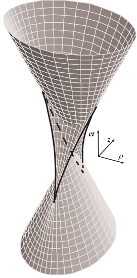
Figure 1: The null hypersurface (95). One dimension is suppressed. The dark solid and dashed lines show its two-dimensional null caustic surface.

The new tangent fields at the two-surface are

$$\tilde{x}^{a}_{v} = -\frac{3}{2}\,a\sin 2v[1,\cos v\cos w,\cos v\sin w,-\sin v]$$

$$\tilde{x}^{a}_{w} = \hphantom{-\frac{3}{2}}\,a\cos^{3}v[0,-\sin w,\cos w,0].$$ (103)

The latter new tangent field coincides with the field obtained as the result of substitution $u=3\cos 2v$ in the expression for $x^{a}_{w}$ in (96), while the former is only a multiple of the null vector field $x^{a}_{u}$ in (96). For this reason and to simplify subsequent calculations, we can equally use the null vector field $x^{a}_{u}$ in order to find the spinor corresponding to the null direction tangent to the two-surface. Since the first tangent vector field $\tilde{x}^{a}_{v}$ has zero Lorentz norm and the second tangent vector field $\tilde{x}^{a}_{w}$ is space-like at the points given by the equation (102), we infer that the two-surface is a null two-surface in 4D Minkowski space-time. The parametric representation (102) also provides a representation for this surface as an intersection of two hypersurfaces:

$$x^{2}+y^{2}+z^{2} = \frac{a^{2}}{4}\left[1+3\left(\frac{4ct}{3a}\right)^{2}\right],$$ (104)

$$x^{2}+y^{2}-z^{2} = \frac{a^{2}}{4}\left(\frac{4ct}{3a}\right)\left[3+\left(\frac{4ct}{3a}\right)^{2}\right].$$

Here $\left|4ct/3a\right|$ $\leq$ $1$. Eliminating $4ct/3a$ from the equations in (104), we observe that in a particular reference frame the projection of this null two-surface in a hyperplane of constant time is an astroid of revolution with the parameter $a$ given by the equation:

$$[x^{2}+y^{2}+z^{2}-a^{2}]^{3}+27a^{2}[x^{2}+y^{2}]z^{2}=0$$ (105)

(see Fig. 2).

As well known, a compact space-like two-surface in 4D Minkowski space-time can be represented as an intersection of two null hypersurfaces. Somewhat analogues to that situation, two-dimensional self-intersections (caustics) of null hypersurfaces provide examples of non-geodesic null two-surfaces in 4D Minkowski space-time.

In order to make connection with the description of the previous sections, we need the spin-tensor expressions of various vector field quantities. As mentioned above, the null vector field $x^{a}_{u}$ can be employed to obtain the spinor field describing the null directions tangent to the null two-surface. First, we explicitly calculate

$$x^{AA^{\prime}}_{u}[\,=x^{a}_{u}(\sigma_{a})^{AA^{\prime}}]=\frac{a}{4\sqrt{2}}\left[\begin{array}[]{ll}1-\sin v&\cos v\,\mbox{e}^{iw}\\ \cos v\,\mbox{e}^{-iw}&1+\sin v\end{array}\right].$$ (106)

[Here $(\sigma_{a})^{AA^{\prime}}$ are the Pauli matrices.] Since the vector field $x^{a}_{u}$ is real-valued and null, the determinant of the matrix in (106) vanishes and we must have $x^{AA^{\prime}}_{u}\propto\bar{\pi}{}^{A}\pi^{A^{\prime}}$. The components of the spinor $\bar{\pi}_{A}$ can be taken as follows:

$$\bar{\pi}_{A}=-i\sqrt{2}\left[\begin{array}[]{r}\cos\left(\frac{v}{2}-\frac{\pi}{4}\right)\mbox{e}^{-iw/2}\\ \sin\left(\frac{v}{2}-\frac{\pi}{4}\right)\mbox{e}^{\,\hskip 5.69054ptiw/2}\end{array}\right].$$ (107)

V.2 Non-geodesic null string

Now we are in a position to explore connections between the example null two-surface and a non-geodesic null string world-sheet in 4D Minkowski space-time, Ilienko2-Zheltukhin . Changing the parameters $(v,w)$ to $(\tau,\sigma)$ we can rewrite the parametric representation (102) for the null two-surface as $x^{a}$ = $a$$[(3/4)\cos 2\tau,$ $\cos^{3}\tau\cos\sigma,$ $\cos^{3}\tau\sin\sigma,$ $\sin^{3}\tau]$. The range of the parameters is $\tau\in$ $[\pi/2,\pi]$ and $\sigma\in$ $[0,2\pi]$. This corresponds to a closed null string with the parameter $\tau$ playing the role of a time variable. The results (106) and (107) allow us to write

$$\dot{x}^{AA^{\prime}}=\frac{3a}{2\sqrt{2}}\sin 2\tau\,\bar{\pi}{}^{A}\pi^{A^{\prime}}.$$ (108)

Here $\bar{\pi}_{A}$ is given by the formula (107) with the necessary change of $(v,w)$ to $(\tau,\sigma)$. Next, we introduce a second spinor field $\bar{\eta}{}^{A}$:

$$\bar{\eta}{}^{A}=\frac{i}{\sqrt{2}}\left[\begin{array}[]{l}\cos\left(\frac{\tau}{2}-\frac{\pi}{4}\right)\mbox{e}^{\hskip 5.69054pti\sigma/2}\\ \,\sin\left(\frac{\tau}{2}-\frac{\pi}{4}\right)\mbox{e}^{-i\sigma/2}\end{array}\right].$$ (109)

which, together with $\bar{\pi}_{A}$, constitutes a normalized Newman-Penrose dyad (spin-frame) for all admissible values of the parameters $\tau$ and $\sigma$. Making the use of (107) and (109) we obtain

$$\acute{x}{}^{AA^{\prime}}=-i\frac{a}{\sqrt{2}}\,\cos^{3}\tau\,(\bar{\pi}{}^{A}\eta^{A^{\prime}}-\bar{\eta}{}^{A}\pi^{A^{\prime}}).$$ (110)

The vector fields $\dot{x}{}^{a}$ and $\acute{x}{}^{a}$ tangent to the null two-surface vanish at two space-time points

$$ct=-\frac{3a}{4},\,\,\,\,x=y=0,\,\,\,\,z=\pm\,a$$ (111)

and, in addition, the vector field $\dot{x}{}^{a}$ vanishes on the circle

$$ct=\frac{3a}{4},\,\,\,\,x^{2}+y^{2}=a^{2},\,\,\,\,z=0.$$ (112)

Comparing the results (108) and (110) with the first two equations in the system (56), we can identify the functions $r$ and $\zeta$ as follows:

$$r=\frac{3a}{2\sqrt{2}}\,\sin 2\tau,\,\,\,\,\zeta=-\frac{a}{\sqrt{2}}\,\cos^{3}\tau.$$ (113)

The expressions for $\bar{\pi}{}^{A}$ and $\bar{\eta}{}^{A}$ can be used to obtain the functions $(\omega-\ln|\zeta|)\dot{}$ and $\psi$ of the Ref. Ilienko2-Zheltukhin directly, the result reads:

$$(\omega-\ln|\zeta|)\dot{}=0,\,\,\,\,\psi=\frac{a}{4\sqrt{2}}\,.$$ (114)

This knowledge is important for relating $\mbox{Re}\,\dot{\omega}$ and $\psi$ with the quantities which represent the field strength of the gauge field $B_{ab}(x)$ of the paper Ilienko2-Zheltukhin . Thus, we obtain

$$\psi = -\frac{3}{4}\,\mbox{\ae}a^{2}\sin 2\tau\cos^{3}\tau(\rho^{\tau})^{-1}\phi,$$

$$2\mbox{Re}\,\dot{\omega} = -\frac{3}{2}\,\mbox{\ae}a^{2}\sin 2\tau\cos^{3}\tau(\rho^{\tau})^{-1}\mbox{Re}\,\nu$$

$$+\left(\ln|\cos^{6}\tau\,(\rho^{\tau})^{-1}|\right)^{.}.$$

Substituting the result (114) in these equations we have

$$\phi = -\,\rho^{\tau}[3\sqrt{2}\mbox{\ae}a\sin 2\tau\cos^{3}\tau]^{-1},$$ (116)

$$\mbox{Re}\,\nu = -\,\rho^{\tau}[\frac{3}{2}\,\mbox{\ae}a^{2}\sin 2\tau\cos^{3}\tau]^{-1}\left(\ln|\cos^{6}\tau\,(\rho^{\tau})^{-1}|\right)^{.}.$$

The formulae above show that the quantity $\phi$ representing the only physical degree of freedom of the field strength diverges at the space-time points (111) and on the circle (112).

Therefore, in a particular reference frame, Fig. 2, one can interpret the null two-surface of this section as a pair of circular null strings which appear with zero radius at $t=-3a/4c$ at spatial points ($x$, $y$, $z$) = ($0$, $0$, $\pm a$). They then expand until the time $t=3a/4c$, when they disappear having the circumference of $2\pi a$. The null strings are the sections of the caustic two-surface in Fig. 1 by the hyperplanes of constant time. Projection of the world-sheets of the null strings into a particular reference frame constitutes the astroid of revolution described earlier in this section.

Figure 2: Null string interpretation of the two-dimensional caustic surface. (a) A section of the two-surface by a hyperplane of constant time (one space dimension is not shown). (b) The space picture of the null strings dynamics.

V.3 Evolution equation

It is also interesting to make connections of this example with the evolution equation for non-geodesic null strings derived in the previous section. The parametric expressions for $\bar{\pi}{}^{A}$ and $\bar{\eta}{}^{A}$, together with the results (108) and (110), can be utilized to verify the equality (82). Noting that $\kappa$ = $r^{-1}$, we find

$$\acute{\kappa}=0,\,\,\,\,\dot{\zeta}=\frac{3a}{2\sqrt{2}}\sin 2\tau\cos\tau\,\,\,\,\mbox{and}\,\,\,\,U-\bar{U}=0.$$ (117)

Then, we have $x\!\!\dot{}\,\acute{}\,{}^{a}$ = $\zeta^{-1}\dot{\zeta}\acute{x}{}^{a}$. Next, the formulae (85) and (86) yield

$$\acute{x}{}^{2} = -\,a^{2}\cos^{6}\tau,\hskip 27.0pt\ddot{x}x\!\!\dot{}\,\dot{}\,\acute{}=0,$$

$$\acute{x}x\!\!\dot{}\,\acute{} = \frac{3}{2}\,a^{2}\sin 2\tau\cos^{4}\tau,\,\,\ddot{x}{}^{2}=-\frac{9}{4}\,a^{2}\sin^{2}2\tau.$$ (118)

Finally, with the aid of results obtained above, we observe that the evolution equation (93) holds.

VI Discussion and Outlook

Firstly, the method employed in this paper for obtaining a variational principle, (10), for a null two-surface can be, in principle, used for designing a twistor variational principle for time-like two-surfaces (conventional strings) and space-like two-surfaces. The idea is to take a simple bivector field $p_{ab}(x)$ and impose one of the algebraic conditions $p_{ab}p{}^{ab}$ = $1$ or $p_{ab}p{}^{ab}$ = $-1$. The latter condition would single out the string (compare with the last part of Gusev-Zheltukhin ), while the former would correspond to a space-like two-surface. It is easy to see that such a procedure uniquely fixes the symmetric second rank spin-tensor field $\phi{}_{AB}(x)$ in the standard decomposition of an antisymmetric 4D Minkowski space-time tensor field $p{}_{ab}(x)=\phi{}_{AB}(x)\varepsilon{}_{A^{\prime}B^{\prime}}+\bar{\phi}{}_{A^{\prime}B^{\prime}}(x)\varepsilon{}_{AB}$. Then, the variational principle

$$S=\frac{1}{2!}\int[\phi{}_{AB}(x)\varepsilon{}_{A^{\prime}B^{\prime}}+\bar{\phi}{}_{A^{\prime}B^{\prime}}(x)\varepsilon{}_{AB}]dx^{AA^{\prime}}\wedge dx^{BB^{\prime}}$$

would define a two-surface subject to the differential constraint stated in Sec. I [see the equation (68)]. Now, one hopes that the use of spinor decomposition for $p_{ab}(x)$, consistent with either of the formulated algebraic constraints, would provide equations of motion, which automatically incorporate the differential constraints formulated in the Sec. I. Such an assertion is supported by the success of this procedure for the null two-surfaces (null strings) presented in the current contribution. It may well be possible to derive the analogues of the evolution equation (93) for generic (interacting) strings in 4D Minkowski space-time and curved space-times of general relativity, where exist explicit spinor and twistor constructions (cf. (Indusy, , Eqn. (16)) and (Flaherty, , Eqns. (3.6)–(3.11))). In the same way it should be possible to build twistor action functionals in the both cases for generic time-like and space-like two-surfaces of 4D Minkowski space-time.

Secondly, if one employs Feber’s definition of a
SU$(2,2\,|\,N)$ supertwistor Feber , one could build a description of null strings with spin in the physical dimensions of space-time. Its analisys presumably would follow the standard pass outlined in the works of Shirafuji Shirafuji and Bengtsson et al. Bengtsson_et_al .

References

• (1) L. Brink, P. Di Vecchia and P. Howe, “A Lagrangian formulation of the classical and quantum dynamics of spinning particles”, Nucl. Phys. B 118, 76 – 94 (1977).
• (2) L.P. Hughston and W.T. Shaw, “Twistors and strings”, in: Twistors in mathematics and physics, Eds. T.N. Bailey and R.J. Baston, LMS Lecture Notes, Vol 156, 218–245 (1990).
• (3) I.A. Bandos i A.A. Zheltukhin, “Kovariantnoe kvantovanie nulp1-super-membran v 4-mernom prostranstve-vremeni”, TMF 88(3), 358–375 (1991).
• (4) S. Kar, “Schild’s null strings in flat and curved backgrounds”, Phys. Rev. D 53, 6842 – 6846 (1996).
• (5) O.E. Gusev i A.A. Zheltukhin, “Tvistornoe opisanie mirovykh plowadok i integral de$\check{\mbox{\cyr i}}$stviya strun”, Pisp1ma ZhE1TF 64(7), 449–455 (1996).
• (6) C.O. Lousto and N. Sánchez, “String dynamics in cosmological and black hole backgrounds: The null string expansion”, Phys. Rev. D 54, 6399 – 6407 (1996).
• (7) M.P. Dabrowski and A.L. Larsen, “Null strings in
Schwarschild spacetime”, Phys. Rev. D 55(10), 6409 – 6414 (1997).
• (8) S. Frittelli, E.T. Newman and G. Silva-Ortigoza, “The eikonal equation in flat-space: null surfaces and their singularities I”, J. Math. Phys. 40, 383 – 407 (1999).
• (9) L. Brink, S. Deser and B. Zumino, P.Di Vecchia and P. Howe, “Local symmetry for spinning particles”, Phys. Lett. B 64(4), 435 – 438 (1976).
• (10) T. Shirafuji, “Lagrangian mechanics of massless particles with spin”, Progr. Theor. Phys. 70(1), 18–35 (1983).
• (11) D.V. Volkov and A.A. Zheltukhin, “Lagrangians for massless particles and strings with local and global supersymmetry”, Nucl. Phys. B 335, 723–739 (1990).
• (12) V.A. Soroka, D.P. Sorokin, V.I. Tkach and D.V. Volkov, “A generalized twistor dynamics of relativistic particles and strings”, Int. J. Mod. Phys. 7(24), 5977–5993 (1992).
• (13) R. Penrose and W. Rindler, “Spinors and space-time”, Vols 1–2, CUP 1984.
• (14) M. Kossowski, “The intrinsic conformal structure and Gauss map of a light-like hypersurface in Minkowski space”, Trans. Am. Math. Soc. 316(1), 369 – 383 (1989).
• (15) A. Ashtekar, C. Beetle, O. Dreyer, S. Fairhurst, B. Krishnan, J. Lewandowski and J. Wiśniewski, “Generic isolated horizons and their applications”, Phys. Rev. Lett. 85, 3564–3567 (2000).
• (16) O. Dreyer, A. Ghosh and J. Wiśniewski, “Black hole entropy calculations based on symmetries”, Preprint hep-th/0101117 (2001).
• (17) R. Penrose, “Twistor geometry of light rays”, Class. Quantum Grav. 14, A299–A323 (1997).
• (18) K.L. Duggal and A. Bejancu, “Lightlike submanifolds of semi-Riemannian manifolds and applications”, Kluwer Academic Publishers 1996.
• (19) A.A. Zheltukhin, “Tension as a perturbative parameter in nonlinear string equations in curved spacetime”, Class. Quantum Grav. 13, 2357 – 2360 (1996).
• (20) A.A. Zheltukhin and U. Linström, “Strings in a space with tensor central charge coordinates”, Preprint hep-th/0103101 (2001).
• (21) A. Schild, “Classical null strings”, Phys. Rev. D 16(6), 1722–1726 (1977).
• (22) A.A. Zheltukhin, “Ob ot ​​​​sut ​​​​stvii vzaimode$\check{\mbox{\cyr i}}$stviya nulp1-strun i nulp1-membran s antisimmetrichnymi polyami”, YaF 51(5), 1504–1513 (1990).
• (23) K. Ilienko, “Null-string dynamics in an external antisymmetric field in Minkowski space-time”, in: Physical applications and mathematical aspects of geometry, groups and algebras, Vol 2, 689–692, Eds. H.-D. Doebner et al., World Scientific, Singapore (1997).
• (24) K. Ilienko and A.A. Zheltukhin, “Tensionless string in the notoph background”, Class. Quantum Grav. 16(2), 383–393 (1999).
• (25) K. Ilyenko, “Twistor description of null strings”, D.Phil. Thesis, University of Oxford (1999).
• (26) J. Stachel, “Thickening the string II. The null-string dust”, Phys. Rev. D 21(8), 2182–2184 (1980).
• (27) J.A. Schouten, “Ricci-calculus”, Springer–Verlag 1954.
• (28) E. Newman and R. Penrose, “An approach to gravitational radiation by a method of spin coefficients”, J. Math. Phys. 3(3), 566–578 (1962).
• (29) E. Noether, “Invariante Variationprobleme”, Nach. v. d. Ges. d. Wiss. zu G$\ddot{\rm{o}}$ttingen, 235–257 (1918).
• (30) B.M. Barbashov and V.V. Nesterenko, “Continuous symmetries in field theory”, Fortschr. Phys. 31(10), 535–567 (1983).
• (31) B. Mukhopadhyay, “Dirac equation in Kerr geometry”, Preprint gr-qc/9910018 (1999).
• (32) E.J. Flaherty, “Complex variables in relativity”, in: General relativity and gravitation, 207–239, Ed. A. Held, Plenum Press, New York (1980).
• (33) A. Feber, “Supertwistors and conformal supersymmetry”, Nucl. Phys. B 132, 55–64 (1978).
• (34) A.K.H. Bengtsson, I. Bengtsson, M. Cederwall and N. Linden, “Particles, superparticles, and twistors”, Phys. Rev. D 36(6), 1766–1772 (1987).