TIFR/TH/01-22 hep-th/0108234
IMSc/2001/07/32    August, 2001

Disc Instantons in Linear Sigma Models

Suresh Govindarajan

Department of Physics, Indian Institute of Technology, Madras,
Chennai 600 036, India
T. Jayaraman

The Institute of Mathematical Sciences,
Chennai 600 113, India
Tapobrata Sarkar

Department of Theoretical Physics,
Tata Institute of Fundamental Research,
Homi Bhabha Road, Mumbai 400 005, India

We construct a linear sigma model for open-strings ending on special Lagrangian cycles of a Calabi-Yau manifold. We illustrate the construction for the cases considered by Aganagic and Vafa(AV). This leads naturally to concrete models for the moduli space of open-string instantons. These instanton moduli spaces can be seen to be intimately related to certain auxiliary boundary toric varieties. By considering the relevant Gelfand-Kapranov-Zelevinsky (GKZ) differential equations of the boundary toric variety, we obtain the contributions to the worldvolume superpotential on the A-branes from open-string instantons. By using an ansatz due to Aganagic, Klemm and Vafa (AKV), we obtain the relevant change of variables from the linear sigma model to the non-linear sigma model variables - the open-string mirror map. Using this mirror map, we obtain results in agreement with those of AV and AKV for the counting of holomorphic disc instantons.

1 Introduction

D-branes have come to play a fundamental role in our understanding of string theory, especially for the case Calabi-Yau (CY) compactifications. Subsequent to the initial description of D-branes wrapping supersymmetric cycles of CY manifolds [1], it was realised that A and B-type D-branes are closely related to the objects that are relevant to Kontsevich’s homological mirror symmetry proposal[2, 3]. The fact that mirror symmetry, generally speaking, exchanges A-branes and B-branes has begun to play a crucial role in understanding several aspects of stringy geometry on Calabi-Yau manifolds.

One of the applications of mirror symmetry in type II compactifications has been the computation of closed string instanton corrections to various physical quantities. With the inclusion of D-brane sectors for strings moving on Calabi-Yau backgrounds, one has, in addition, to consider a generalisation of mirror symmetry that also includes the open string sectors. In particular, one may expect that mirror symmetry in the open and closed string sectors taken together is relevant to understanding the contribution of open-string instanton corrections.

In contrast to the case of purely closed strings on CY, it has been pointed out that various quantities in the world-volume theories of both A and B type D-branes acquire open-string instanton corrections. In general it is expected that the F-terms in the world-volume theory have open-string instanton corrections for A-branes whereas the D-terms are the ones that acquire instanton corrections for B-branes[4, 5]. Various general considerations relevant to open-string instanton corrections in the case of compact Calabi-Yau manifolds as well as non-compact Calabi-Yau manifolds have been studied earlier[6, 7].

However the explicit calculation of open-string instanton corrections to the world-volume superpotential for A-branes using mirror symmetry have first appeared recently in the important work of Aganagic and Vafa [8] and Aganagic, Klemm and Vafa[9]. The authors in these papers have computed the world-volume superpotential for some non-compact A-branes in non-compact Calabi-Yau manifolds (in particular, those that can be described without a world-sheet superpotential), by appealing to mirror symmetry and using the holomorphic Chern-Simons action on the B-brane side to reduce the problem to a more tractable computation. This computation uses and extends the techniques first described in [10, 11], whereby the mirror transformation, in the presence of D-branes, can be explicitly implemented as a world-sheet duality transformation involving the fields of a Gauged Linear Sigma Model (GLSM) that describes these D-brane configurations. Remarkably, the authors of [8, 9] showed that the (instanton generated) A-brane superpotential thus computed conformed exactly to the strong integrality predictions of such quantities from completely different considerations of large $N$ duality [12].

We briefly recall here the manner in which this integrality predictions were first made. In [13] it was conjectured that the large $N$ limit of Chern-Simons theory on $S^{3}$ is dual to A-type closed topological string theory on the resolved conifold, with a particular identification between the parameters of the two theories. This conjecture was verified at the level of the partition function on both sides. The conjecture was extended to the observables of the Chern-Simons theory, namely the knot invariants in [12]. By identifying the extra D-branes (associated with the knots on the Chern-Simons side) on the resolved conifold, non-trivial predictions were made in [12] regarding the structure of the topological string amplitudes, using ideas of [15]. (Knot theoretic aspects of the conjecture were verified in [14].) Further, from the fact that topological disc amplitudes compute superpotential terms in $N=1$ $d=4$ gauge theories, a general structure for the A-type superpotential was proposed, which had the integrality properties that we referred to above.

It is of interest to ask the question whether the A-brane world-volume superpotential, together with the open-string instanton corrections, can be directly computed without explicit recourse to mirror symmetry, particularly in the framework of the GLSM[16]. In this paper, we will take the first steps in this direction. We will show that the description of the A-branes in the linear sigma model framework suggests a natural and concrete description of these (partially compactified) open-string instanton moduli spaces. These instanton moduli spaces will be seen to be intimately related to some auxiliary toric varieties that we shall refer to as boundary toric varieties. For these boundary toric varieties we will write down the appropriate Gelfand-Kapranov-Zelevinsky (GKZ) differential equations, by an extension of the methods developed for the closed string case, particularly for non-compact CY manifolds by [17, 18]. We will then show how the relevant solutions of the GKZ equations describe the world-volume superpotential for the A-branes in the examples considered by [8, 9]. We will also show how to obtain the analogue of the open-string mirror map in this context, using in part, an ansatz due to Aganagic, Klemm and Vafa.

This paper is organised as follows. In section 2, we describe some basic facts about the Gauged Linear Sigma Model. After describing the construction of A and B-type superspace, we discuss the boundary conditions of [8] that describes A-branes. In section 3, we discuss the GLSM for A-branes and the boundary conditions therein. In section 4, we discuss the topological aspects of the A-model, before moving on, in section 5, to the open string instanton moduli space. After discussing briefly certain issues of stability, we introduce the boundary toric variety. In section 6, we consider aspects of local mirror symmetry and the GKZ system of equations for our boundary toric variety. We discuss how to obtain the bulk and boundary periods that are relevant for the computation of the A-brane superpotential in the mirror. Section 7 deals with some examples in order to illustrate the methods. We conclude with some observations in section 8.

2 Background

The supersymmetry generators for $(2,2)$ supersymmetry can be written as (in the notation of [16])

$$\delta_{susy} = \epsilon^{\alpha}Q_{\alpha}+\bar{Q}_{\dot{\alpha}}\epsilon^{\dot{\alpha}}$$ (2.1)

$$= -\epsilon_{-}Q_{+}+\epsilon_{+}Q_{-}+\bar{\epsilon}_{-}\bar{Q}_{+}-\bar{\epsilon}_{+}\bar{Q}_{-}$$

In superspace with coordinates $(x^{m},\theta^{\pm},\bar{\theta}^{\pm})$, the supersymmetry generators have the following representation

$$Q_{\pm} = {\partial\over{\partial\theta^{\pm}}}+i\bar{\theta}^{\pm}(\partial_{0}\pm\partial_{1})$$

$$\bar{Q}_{\pm} = -{\partial\over{\partial\bar{\theta}^{\pm}}}-i\theta^{\pm}(\partial_{0}\pm\partial_{1})$$ (2.2)

On the boundary, one set of linear combinations of this supersymmetry is preserved. Let us denote the unbroken supersymmetry generators by $Q$ and $\bar{Q}$. Let us denote the boundary in superspace by the coordinates $(x^{0},\theta,\bar{\theta})$. Then, the supersymmetry generators can be given the following representation

$$Q={\partial\over{\partial\theta}}+i\overline{\theta}\partial_{0}\quad,\quad\overline{Q}=-{\partial\over{\partial\overline{\theta}}}-i\theta\partial_{0}\quad,$$ (2.3)

We will now work out the precise relationship between the boundary coordinates/ supersymmetry generators. We will deal with the A- and B-type cases separately.

A-type superspace

Under A-type supersymmetry, let

$$\epsilon_{A}\equiv-\sqrt{2}\epsilon_{-}=-\sqrt{2}\eta\bar{\epsilon}_{+}\quad,$$

where we use the subscript $A$ to denote that we are considering boundaries that preserve A-type supersymmetry. Then, on using

$$\delta_{A} \equiv \epsilon_{A}Q_{A}-\bar{\epsilon}_{A}\bar{Q}_{A}$$ (2.4)

$$= -\bar{\epsilon}_{+}(\bar{Q}_{-}+\eta Q_{+})+\epsilon_{+}(Q_{-}+\eta\bar{Q}_{+})\quad,$$

we obtain

$$Q_{A}=\left({{Q_{+}+\eta\bar{Q}_{-}}\over\sqrt{2}}\right)\quad{\rm and}\quad\theta_{A}\equiv\sqrt{2}\theta^{+}=-\sqrt{2}\eta\bar{\theta}^{-}\quad.$$

B-type superspace

In a similar fashion one chooses $\epsilon_{B}\equiv\sqrt{2}\epsilon_{-}=\sqrt{2}\eta\epsilon_{+}$.

$$\delta_{B} = \epsilon_{B}\left({{-Q_{+}+\eta Q_{-}}\over\sqrt{2}}\right)-\bar{\epsilon}_{B}\left({{-\bar{Q}_{+}+\eta\bar{Q}_{-}}\over\sqrt{2}}\right)$$ (2.5)

$$\equiv \epsilon_{B}Q_{B}-\bar{\epsilon}_{B}\bar{Q}_{B}\quad,$$

from which we identify

$$Q_{B}={{-Q_{+}+\eta Q_{-}}\over\sqrt{2}}\quad{\rm and}\quad\theta_{B}\equiv-\sqrt{2}\theta^{+}=\sqrt{2}\eta\theta^{-}\quad.$$

2.1 Boundary multiplets

In boundary superspace with coordinates $(x^{0},\theta,\bar{\theta})$, the superderivatives are

$$D={\partial\over{\partial\theta}}-i\overline{\theta}\partial_{0}\quad,\quad\bar{D}=-{\partial\over{\partial\overline{\theta}}}+i\theta\partial_{0}\quad.$$ (2.6)

We will deal with two kinds of boundary multiplets: a boundary chiral multiplet and an unconstrained complex multiplet.

A boundary chiral multiplet satisfying the constraint

$$\bar{D}L=0\quad,$$

which has the following component expansion

$$L=l+i\theta\lambda-i\theta\bar{\theta}\partial_{0}l\quad.$$

An unconstrained complex superfield $U$ with component expansion

$$U=u+\theta\upsilon-\bar{\theta}\xi+\theta\bar{\theta}(D^{\prime}+iR)$$ (2.7)

where $D^{\prime}$ and $R$ are real fields. Under supersymmetry, the transformations are

$$\delta u = -\bar{\epsilon}\xi+\epsilon\upsilon$$

$$\delta\upsilon = -\bar{\epsilon}(-i\partial_{0}u+D^{\prime}+iR)$$ (2.8)

$$\delta\xi = -\epsilon(i\partial_{0}u+D^{\prime}+iR)$$

$$\delta(D^{\prime}+iR) = -i\epsilon\partial_{0}\upsilon-i\bar{\epsilon}\partial_{0}\xi$$

Now consider a complex superfield with the following gauge invariance

$$U\rightarrow U+L$$ (2.9)

where $L$ is a chiral superfield. A gauge-invariant observable is given by $\Xi\equiv\bar{D}U$. The invariance trivially follows from the chirality of $L$. $\Xi$ has the following superfield expansion

$$\Xi=\bar{D}U=\xi+\theta(D^{\prime}+iR+i\partial_{0}u)-i\theta\bar{\theta}\partial_{0}\xi\quad,$$ (2.10)

We will identify the real part of $U$ with the bosonic $u$ discussed earlier. Keeping this in mind, we can partially gauge-fix the imaginary part of $U$ as follows

$${\rm Im}(U)=\theta\bar{\theta}(R)\quad.$$ (2.11)

Note that the gauge choice is algebraic and hence we will call it the Wess-Zumino (WZ) gauge. This leaves us with the following gauge invariance which acts as

$$\delta{\rm Re}(u)={\rm Re}(l)$$

$$\delta R=-\partial_{0}{\rm Re}(l)$$ (2.12)

In the WZ gauge, the field $U$ has the following superfield expansion

$$U=u+\theta\bar{\xi}-\bar{\theta}\xi+\theta\bar{\theta}(D^{\prime}+iR)$$ (2.13)

where $u$ is now a real field. Thus, if $R=0$, it would be a real superfield.

The supersymmetry and gauge transformations which preserve the WZ gauge are

$$\delta u = -\bar{\epsilon}\xi+\epsilon\bar{\xi}+l$$

$$\delta\xi = -\epsilon(i\partial_{0}u+D^{\prime}+iR)$$ (2.14)

$$\delta D^{\prime} = -i\epsilon\partial_{0}\bar{\xi}-i\bar{\epsilon}\partial_{0}\xi$$

$$\delta R = -\partial_{0}l$$

where $l$ is now a real parameter. Notice that $R$ is invariant under supersymmetry and transforms as $-\partial_{0}l$ under gauge transformations and thus behaves as a gauge field.

2.2 Decomposition of bulk multiplets: A-type

First, consider a chiral superfield $\Phi$ which has the following component expansion:

$$\Phi = \phi+\sqrt{2}\theta^{+}\psi_{+}+\sqrt{2}\theta^{-}\psi_{-}+2\theta^{+}\theta^{-}F-i\theta^{+}\bar{\theta}^{+}(D_{0}+D_{1})\phi$$ (2.15)

$$- i\theta^{-}\bar{\theta}^{-}(D_{0}-D_{1})\phi+i\theta^{-}\bar{\theta}^{+}\sqrt{2}Q\sigma\phi-i\theta^{+}\bar{\theta}^{-}\sqrt{2}Q\bar{\sigma}\phi$$

$$- i\sqrt{2}\theta^{+}\theta^{-}\bar{\theta}^{-}[(D_{0}-D_{1})\psi_{+}+\sqrt{2}Q\bar{\sigma}\psi_{-}]$$

$$+ i\sqrt{2}\theta^{+}\theta^{-}\bar{\theta}^{+}[(D_{0}+D_{1})\psi_{-}+\sqrt{2}Q\sigma\psi_{+}]$$

In order to obtain the A-type superfield, we need to set $\theta\equiv\sqrt{2}\theta^{+}=-\sqrt{2}\eta\bar{\theta}^{-}$ Thus, we obtain

$$\Phi^{\prime}\equiv\Phi|_{\theta^{+}=-\eta\bar{\theta}^{-}}=\phi+\theta\psi_{+}-\eta\bar{\theta}\psi_{-}-\theta\bar{\theta}(\eta F+iD_{1}\phi)$$ (2.16)

where the prime indicates an A-type superfield. This is a complex unconstrained superfield.

Next, let us consider a twisted chiral superfield $\Sigma$ which has the following component expansion

$$\Sigma = \sigma+i\sqrt{2}\theta^{+}\bar{\lambda}_{+}-i\sqrt{2}\bar{\theta}^{-}\lambda_{-}+\sqrt{2}\theta^{+}\bar{\theta}^{-}(D-iv_{01})$$ (2.17)

$$- i\bar{\theta}^{-}\theta^{-}(\partial_{0}-\partial_{1})\sigma-i\theta^{+}\bar{\theta}^{+}(\partial_{0}+\partial_{1})\sigma+\sqrt{2}\bar{\theta}^{-}\theta^{+}\theta^{-}(\partial_{0}-\partial_{1})\bar{\lambda}_{+}$$

$$+ \sqrt{2}\theta^{+}\bar{\theta}^{-}\bar{\theta}^{+}(\partial_{0}+\partial_{1})\lambda_{-}-\theta^{+}\bar{\theta}^{-}\theta^{-}\bar{\theta}^{+}(\partial_{0}{}^{2}-\partial_{1}{}^{2})\sigma.$$

We define the A-type superfield $\Sigma^{\prime}$ as in the case of the chiral superfield. We obtain

$$\Sigma^{\prime}\equiv\Sigma|_{\theta^{+}=-\eta\bar{\theta}^{-}}=\sigma+i\theta(\bar{\lambda}_{+}+\eta\lambda_{-})-i\theta\bar{\theta}\partial_{0}\sigma$$ (2.18)

which is the superfield expansion for an A-type chiral superfield. In addition, one obtains a Fermi chiral superfield $\Lambda$ whose lowest component is $\lambda\equiv(\bar{\lambda}_{+}-\eta\lambda_{-})$ satisfying

$$\bar{D}\Lambda=2\partial_{1}\Sigma^{\prime}\quad,$$ (2.19)

where one treats $\partial_{1}\Sigma^{\prime}$ as an A-type chiral superfield with lowest component $\partial_{1}\sigma$. The component expansion for $\Lambda$ is

$$\Lambda=(\bar{\lambda}_{+}-\eta\lambda_{-})+i\sqrt{2}\theta(D-iv_{01})-2\overline{\theta}\partial_{1}\sigma+\theta\overline{\theta}\left[-i\partial_{0}(\bar{\lambda}_{+}-\eta\lambda_{-})+2i\partial_{1}(\bar{\lambda}_{+}+\eta\lambda_{-})\right]$$ (2.20)

Something interesting happens if $D-iv_{01}$ is set to zero on the boundary (part of which we know is required by the vanishing of ordinary variations). Then, using the bulk equations of motion for the $\lambda$’s, one can see that $\Lambda$ becomes an anti-chiral boundary superfield.

2.3 The AV boundary conditions

Aganagic and Vafa[8] have constructed a class of special Lagrangian(sL) cycles in toric varieties by adapting the construction of Harvey and Lawson in $\mathbb{C}^{n}$. We shall describe this construction in the language of the GLSM. Let $\Phi_{i}$ ($i=1,\ldots,n$) be the chiral superfields with $U(1)$ charges $Q_{i}^{a}$ which appear in the gauged linear sigma model associated with the toric variety. The toric variety is obtained by imposing the (bulk) D-term constraint given by

$${D^{a}\over{e^{2}}}=r^{a}-\sum_{i}Q^{a}_{i}|\phi_{i}|^{2}=0$$ (2.21)

where $a=1,\ldots,h_{1,1}$. After taking into account the gauge invariances involved, one ends up with some weighted projective space (actually, a line bundle on that space) of dimension $(n-h_{1,1})$. This is the standard procedure called symplectic reduction. The Calabi-Yau condition is given by $\sum_{i}Q_{i}^{a}=0$.

Lagrangian submanifolds in $\mathbb{C}^{n}$ are specified by the following D-term like conditions

$$\sum_{i}q_{i}^{\alpha}|\phi_{i}|^{2}=c^{\alpha}\qquad\alpha=1,\ldots,r$$ (2.22)

Note however that there is no associated local $U(1)$ invariance as occurs in symplectic reduction. One further imposes $(n-r)$ additional conditions on linear combinations of the phases ${\rm Im}\log\phi_{i}$ of the fields $\phi_{i}$

$$\sum_{i}v^{\beta}_{i}\ {\rm Im}\log\phi_{i}=0\quad\beta=1,\ldots,(n-r)$$ (2.23)

The $(q^{\alpha},v^{\beta})$ specify a Lagrangian submanifold of $\mathbb{C}^{n}$ (with the standard symplectic structure) if

$$\sum_{i}q^{\alpha}_{i}v^{\beta}_{i}=0\quad.$$

In order for this Lagrangian submanifold in $\mathbb{C}^{n}$ to descend to the toric variety, we choose $h_{1,1}$ of the conditions given above to be the D-term conditions associated with the toric variety. The conditions $\sum_{i}Q^{a}_{i}v^{\beta}_{i}=0$ imply that the conditions on the phases are invariant under $U(1)$ gauge transformations. Further, it follows that the submanifold is special Lagrangian if

$$\sum_{i}q^{\alpha}_{i}=0\quad.$$

This is clearly compatible with the Calabi-Yau condition on the bulk $U(1)$ charges.

For generic values of $c^{\alpha}$, the sL submanifolds have a boundary. One can obtain sL submanifolds without boundary by a doubling procedure. However, there exist non-generic situations (such as the case when one of the $c^{\alpha}$ vanish) where the doubling is not necessary. In other words, when we take an sL submanifold without boundary for generic values of $c^{\alpha}$ to the non-generic value, the sL manifold splits into two. We shall refer to one component as an half-brane following AV[8]. In the toric description, half-branes lie on the edges of toric skeletons.

In order to be more concrete, let us consider a specific example furnished by the non-compact Calabi-Yau manifold given by the total space of the line-bundle ${\cal O}(-3)$ over $\mathbb{P}^{2}$. This non-compact Calabi-Yau manifold is described in the GLSM by four fields with $U(1)$ charge $Q=(-3,1,1,1)$ and the boundary conditions of the special Lagrangian submanifold are given by $q^{1}=(-1,1,0,0)$, $q^{2}=(-1,0,1,0)$ and $v=(1,1,1,1)$. For generic values of $c^{\alpha}$, the topology of the sL submanifolds (after doubling) is $\mathbb{R}\times S^{1}\times S^{1}$. However, for suitable choices of $c^{\alpha}$ (see below), one obtains half-branes which are topologically $\mathbb{C}\times S^{1}$,

Following the discussion in AKV[9], there are three phases (half-branes) of interest: Phase I given by $c^{2}=0$ and $0<c^{1}<r$, Phase II given by $c^{1}=0$ and $0<c^{2}<r$ and Phase III is given by $c^{1}=c^{2}$ and $c^{1}<0$. The relevant phase diagram is as follows

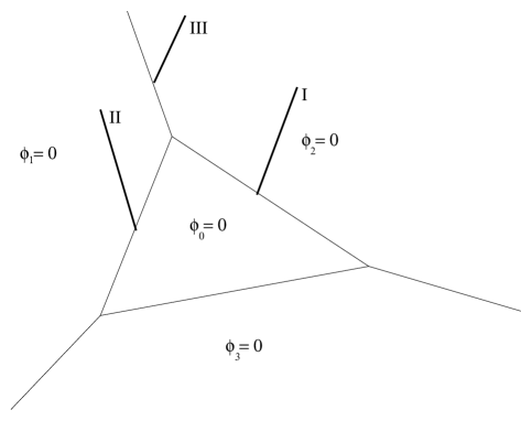
Figure 1: Phases (half-branes) for ${\cal O}(-3)$ on $\mathbb{P}^{2}$

In phase I, for large values of $c^{1}$ and $r$ when quantum corrections are small, $c^{1}$ measures the size of a holomorphic disc ending on the half-brane. This is the real part of a complex modulus, $\widehat{w}^{1}$, whose imaginary part corresponds to turning on a Wilson line wrapping the $S^{1}$ of the half-brane. $\widehat{w}^{2}$ is the other modulus associated with the other $S^{1}$ which appears for generic values of $c^{\alpha}$ vanishes on the half-brane. These values suffer quantum corrections which become relevant for small values of $c^{1}$ and $r$. We will denote the quantum corrected quantities by unhatted quantities. However, $w^{2}$ will not be independent and will be determined as a function of $w^{1}$ on the half-brane.

2.4 The AV/AKV computation of the A-brane Superpotential

As we mentioned in the introduction, the essential idea of [8, 9] is to compute the superpotential for the A-branes described in the last subsection by using mirror symmetry to calculate this in the B-model. Here, we will briefly review their arguments. We will be interested in the case of a space-filling D6-brane wrapping a sL cycle of a non-compact CY three-fold.

It was shown in [12] that the amplitude of interest, the (instanton generated) disc amplitude in the A-model, is of the form

$$W=\sum_{n=0}^{\infty}\sum_{{\vec{m}},{\vec{k}}}\frac{d_{{\vec{m}},{\vec{k}}}}{n^{2}}q^{n{\vec{k}}}\hat{s}^{n{\vec{m}}}$$ (2.24)

where $\hat{s}^{\alpha}=e^{-\widehat{w}^{\alpha}}$, $\widehat{w}^{\alpha}$ is the (complexified) volume of the holomorphic disc with boundary ending on a particular one-cycle on the sL submanifold and $q^{a}=e^{-t^{a}}$, $t^{a}$ being the closed string Kähler class. ${\vec{m}}$ are the winding numbers associated with the holomorphic disc i.e., an element of $H_{1}$ of the sL submanifold and ${\vec{k}}$ is an element of $H_{2}$ of the CY. The integer $n$ relates to the multiple coverings of these. Further, this prediction involves the highly non-trivial integers $d_{{\vec{m}},{\vec{k}}}$, that count the number of primitive disc instantons in this homology class. These have the interpretation of counting the degeneracy of domain wall D4-branes ending on the space-filling D6-brane[12], which wrap a 2-cycle in the CY (whose Kähler class is given by $\vec{k}$) and $\vec{m}$ denotes the wrapping number around the boundary.

Since a direct computation of the superpotential in the A-model involves summing up open-string instantons, AV and AKV use the mirror map of [10] to map this computation to one involving holomorphic Chern-Simons theory in the mirror B-model. For the case when the B-brane is of complex dimension one, and wraps a Riemann surface $C$ in the mirror CY, the dimensional reduction of the Chern-Simons theory on $C$ was computed in [8] in terms of the holomorphic three-form of the Chern-Simons theory restricted to the brane and two scalar fields (denoted by $u$ and $v$ parametrising normal deformations of the B-brane in the mirror CY. The final result for the superpotential is given by the the Abel-Jacobi map associated with the one-form $vdu$

$$W(u)=\int_{u^{*}}^{u}v(u)du$$ (2.25)

where $u^{*}$ is the ‘location’ of the half-brane. $v$ is fixed on the B-model side by the condition that $(u,v)$ be points on the Riemann surface $C$. However, from the A-model viewpoint, it suffices to note that

$$v=\partial_{u}W(u)$$ (2.26)

which is obtained from the Abel-Jacobi map.

There are a couple of issues that one has to address before one can translate these results in the B-model to the A-model side. First, there is an $SL(2,\mathbb{Z})$ ambiguity in the parametrisation of the B-model variables given by

$$\pmatrix{u\cr v}\rightarrow\pmatrix{a&b\cr c&d}\pmatrix{u\cr v}\quad.$$ (2.27)

Thus, the superpotential given above is also dependent on the choice of $u$ and $v$. Second, the variables which appear in the B-model side are not the same as the ones that appear in the A-model. The change of variables that relates the two is the open-string mirror map.

However, in the limit where quantum corrections are suppressed in the A-model, i.e., where the volumes of the holomorphic disc and the CY are large, one can relate the two sets of variables. However, the condition that Re($u$) be the volume of the holomorphic disc and $v\rightarrow 0$ in this limit, breaks the $SL(2,\mathbb{Z})$ down to the subgroup given by

$$\pmatrix{u\cr v}\rightarrow\pmatrix{1&n\cr 0&1}\pmatrix{u\cr v}\quad.$$ (2.28)

Thus, imposing the classical limit leaves us with an ambiguity parametrised by the integer $n$. It turns out that for cases where the A-model is dual to large $N$ Chern-Simons theory[13, 15, 12], this integer reflects a framing ambiguity in the Chern-Simons theory.

The framing ambiguity has recently been studied in the context of the Wilson loop variables of Chern-Simons theory in [23], and evidence has been found that the above mentioned duality is more appropriate in the context of $U(N)$ Chern-Simons theories rather than the $SU(N)$ ones originally considered in the proposal of [12]. Initial works on Knot invariants were insensitive to this because the computations were performed in the standard framing, where the $U(N)$ and $SU(N)$ Knot invariants are the same. However, hints of this had already appeared in [24]. In [23], explicit computations of certain $U(N)$ Wilson loop operators have been carried out, and the results have been shown to conform to the integrality predictions of [12].

Aside from the ambiguity mentioned above, one has to obtain the open-string mirror map in order to obtain the A-model results. It has been argued in AKV that the appropriate variables are given by[9]

$$\hat{u} = u+\Delta(\vec{q})$$ (2.29)

$$\hat{v} = {{\partial W}\over{\partial\hat{u}}}$$ (2.30)

where $\hat{u}$ receives corrections only from closed-string instantons. $\hat{u}$ is computed by identifying it with the tension of the domain wall which is mirror to the D4-brane in the A-model. The variables $u$ and $v$ are conjugate fields of the holomorphic Chern-Simons theory. The second equation corresponds to the condition that $\hat{v}$ remains conjugate to $\hat{u}$ in the quantum theory.

As we will see in the next section, the B-model variables, i.e., the unhatted variables, naturally appear in the GLSM that we construct to describe these half-branes.

3 Linear Sigma Models for A-branes

3.1 The basic boundary condition

The basic A-type boundary conditions that one considers in a GLSM with $n$ chiral superfields and $r$ $U(1)$ vector multiplets are

$${{D^{a}}\over{e^{2}}}=r^{a}-\sum_{i}Q_{i}^{a}|\phi_{i}|^{2}=0\quad a=1,\ldots,r$$ (3.1)

The bosonic boundary conditions (in the matter sector) are completed by the following $(n-r)$ conditions

$$\sum_{i}v^{b}_{i}\ {\rm Im}\log\phi_{i}=0\quad b=1,\ldots,(n-r)$$ (3.2)

where the Lagrangian condition implies that the $v$’s satisfy

$$\sum_{i}v^{b}_{i}\ Q_{i}^{a}=0\quad.$$

This condition permits us to identify, in the toric description, the $v^{b}_{i}$ with the integral generators of the one-dimensional cones in the fan $\Delta$, the combinatoric data associated with the toric variety.

The boundary conditions on the vector multiplet are given by the superfield condition

$$\Sigma_{a}^{\prime}=0$$ (3.3)

The easy way to understand this is to notice that in the topological A-model, the field $\sigma$ is proportional to the Kähler form $\omega$ whose restriction on a Lagrangian submanifold is zero. The vanishing of the boundary terms in the ordinary variation is obtained by the conditions

$$v_{01}^{a}=0$$ (3.4)

The above set of boundary conditions form a consistent set of boundary conditions in the GLSM which also have a proper NLSM limit in the sense used in [19, 20]. Let us denote by $|{\cal B}\rangle_{0}$ the boundary state (in the GLSM) that corresponds to these boundary conditions.

This reference state plays a role similar to the D6-brane in the context of B-branes in the GLSM[21, 22]. It is not hard to see that it corresponds to the D6-brane in the mirror Calabi-Yau manifold. It is also rigid i.e., there are no moduli associated with this sL submanifold.

3.2 The AV boundary conditions in the GLSM

The boundary conditions that AV choose can be implemented in the GLSM in a simple fashion. In the matter sector, it corresponds to simply replacing some of the $v$’s by boundary conditions of the form

$$\sum_{i}q_{i}^{\alpha}|\phi_{i}|^{2}=c^{\alpha}$$

In the GLSM, we will realise these boundary conditions as low-energy conditions using complex boundary supermultiplets $U_{\alpha}$. The corresponding boundary state can be represented by the path-integral

$$|{\cal B}\rangle_{AV}=\int[DU]\ \exp(S_{1}+S_{2}+S_{3})\ |{\cal B}\rangle_{0}$$ (3.5)

where

$$S_{1}=\int dx^{0}d^{2}\theta\left(\sum_{i}q_{i}^{\alpha}\bar{\Phi}^{\prime}_{i}\Phi^{\prime}_{i}\right)\left[\left({{U_{\alpha}+\bar{U}_{\alpha}}\over 2}\right)-\sum_{j}\tilde{q}_{\alpha}^{j}{\rm Im}\log\Phi_{j}^{\prime}\right]$$ (3.6)

This action is invariant under the gauge-invariances

$$U_{\alpha} \rightarrow U_{\alpha}+L_{\alpha}$$ (3.7)

$${\rm Im}\log\Phi^{\prime}_{i} \rightarrow {\rm Im}\log\Phi^{\prime}_{i}+q_{i}^{\alpha}\left({{L_{\alpha}+\bar{L}_{\alpha}}\over 2}\right)\quad.$$ (3.8)

where $L_{\alpha}$ are chiral superfields. This gauge invariances enable us to identify the real parts of the lowest components of the superfields $U_{\alpha}$ and with “coordinates” on an appropriate three-cycle. The action $S_{1}$ is also invariant under bulk gauge transformations. On using the fact that $D^{a}$ are generators of the bulk gauge invariance, one obtains that

$$D^{a}|{\cal B}\rangle_{AV}=0\quad,$$

given that $S_{2}$ and $S_{3}$ (given below) are also gauge-invariant.

The kinetic energy for $\Xi_{\alpha}\equiv\bar{D}U_{\alpha}$

$$S_{2} = -{1\over{2e_{b}^{2}}}\int dx^{0}d^{2}\theta\ \bar{\Xi}_{\alpha}\Xi_{\alpha}$$ (3.9)

$$= {1\over e_{b}^{2}}\int dx^{0}\left(i\bar{\xi}_{\alpha}\partial_{0}\xi_{\alpha}+{1\over 2}(D^{\prime}_{\alpha})^{2}+{1\over 2}(R_{\alpha}+\partial_{0}u_{\alpha})^{2}\right)$$

where we have introduced the coupling constant $e_{b}$ on the boundary. This has mass dimension half.

We can now introduce the boundary analogue of the F.I. term:

$$S_{3}=-{\rm Re}\left(w^{\alpha}\int dx^{0}d\theta\ \Xi_{\alpha}\right)=-\int dx^{0}\left(c^{\alpha}D^{\prime}_{\alpha}-{\theta^{\alpha}\over{2\pi}}(R_{\alpha}+\partial_{0}u_{\alpha})\right)$$ (3.10)

where $w^{\alpha}=c^{\alpha}+i{\theta^{\alpha}\over{2\pi}}$ is a complex parameter.

3.3 Taking $e_{b}\rightarrow\infty$

In the limit $e_{b}\rightarrow\infty$, the fields in the multiplet $\Xi_{\alpha}$ impose the constraints

$${D_{\alpha}^{\prime}\over e_{b}^{2}}=c^{\alpha}-\sum_{i}q_{i}^{\alpha}|\phi_{i}|^{2}=0$$

$$\sum_{i}q_{i}^{\alpha}\left(\overline{\phi}_{i}\psi_{+i}+\eta\phi_{i}\overline{\psi}_{-i}\right)=0$$ (3.11)

$$\sum_{i}q_{i}^{\alpha}\left(\overline{\phi}_{i}\psi_{-i}+\eta\phi_{i}\overline{\psi}_{+i}\right)=0$$

$$\eta\sum_{i}q_{i}^{\alpha}(\bar{\phi}_{i}F_{i}+\phi_{i}F^{*}_{i})+i\sum_{i}q_{i}^{\alpha}(\bar{\phi}_{i}D_{1}\phi_{i}-\phi_{i}D_{1}\bar{\phi}_{i})=0\quad.$$

The last three equations are the supersymmetric variation of the first equation.

The $\theta^{\alpha}$ term is a topological term as one expects. Thus, we can see that the real part of $R$ behaves like the bulk $D$ term while the imaginary part should behave like $v_{01}$. In order for this correspondence to work, we should require that (after Wick rotation to Euclidean space and $x^{0}$ becomes a circle variable which we will call $x^{2}$ with periodicity $2\pi$)

$$\int{{dx^{2}}\over{2\pi}}(R_{\alpha}+\partial_{2}u_{\alpha})=-m_{\alpha}$$

where $m_{\alpha}$ are some integers.

4 The topological version of the GLSM

In order to discuss the topological aspects of the A-model, we need to Wick rotate: $x^{0}\rightarrow-ix^{2}$ (Hence one has $\partial_{0}\rightarrow i\partial_{2}$, $R\rightarrow iR$ and $v_{01}\rightarrow-iv_{12}$). Let us choose to twist the model so that $\bar{Q}$ is the BRST operator. For the closed string case, the localisation equations are[16] $(a=1,\cdots,h_{1,1})$.

$$(D_{1}+iD_{2})\phi=0$$

$$D^{a}+v_{12}^{a}=0$$ (4.1)

$$F_{i}=0$$

$$\sigma^{a}=0$$

Let $n_{a}$ be the instanton numbers defined by

$$n_{a}\equiv-{1\over{2\pi}}\int_{D}d^{2}x\ v_{12}^{a}$$ (4.2)

The action is then equal to

$$S_{\rm bulk}=-2\pi it^{a}n_{a}$$ (4.3)

where $t^{a}={\theta^{a}\over{2\pi}}+ir^{a}$.

In the open-string sector, one obtains

$$D_{\alpha}^{\prime}+(R_{\alpha}+\partial_{2}u_{\alpha})=0$$

$$\xi_{\alpha}=0$$ (4.4)

in addition to the boundary condition

$$\sum_{i}v^{\beta}_{i}{\rm Im}\log\phi_{i}=0\quad.$$ (4.5)

The winding numbers are defined by

$$m_{\alpha}=-{1\over{2\pi}}\int_{\partial D}(R_{\alpha}+\partial_{2}u_{\alpha})$$ (4.6)

The contribution of the boundary terms to the action is

$$S_{\rm bdry}=-2\pi is^{\alpha}m_{\alpha}$$ (4.7)

Thus, the total action in the topological theory is given by

$$S=S_{\rm bulk}+S_{\rm bdry}=-2\pi it^{a}n_{a}-2\pi is^{\alpha}m_{\alpha}\quad.$$

4.1 Observables in the topological theory

The gauge-invariant BRST closed observables in the closed string sector are $\sigma^{a}$. These have ghost number two. In the open-string sector, the observables in the NLSM limit should be in one-to-one correspondence with closed forms on the Lagrangian submanifold. In the AV construction, we assume that a subset of closed one-forms is given by $du_{\alpha}$, where we consider $u_{\alpha}$ to be (compact) coordinates (angles) on the Lagrangian submanifold. Thus, in the topological model, the corresponding observables are $\xi_{\alpha}$ (which are naively BRST exact). Thus one has

	Observable	Ghost No.
Bulk	$\sigma^{a}$	$2$
Boundary	$\xi_{\alpha}$	$1$

5 The open-string instanton moduli space

The open-string instanton moduli space can be defined to be the moduli space of the localisation equations that we derived in the previous section. We assume that the worldsheet is a disc. The relevant equations are:

$$(D_{1}+iD_{2})\phi_{i}=0$$ (5.1)

$$D^{a}+v_{12}^{a}=0$$ (5.2)

$$\left.D_{\alpha}^{\prime}+(R_{\alpha}+\partial_{2}u_{\alpha})\right|_{\partial D}=0$$ (5.3)

$$\sum_{i}v_{i}^{\beta}{\rm Im}\log\phi_{i}|_{\partial D}=0$$ (5.4)

The first two equations are bulk equations while the last two equations are on the boundary of the disc. Thus, we are interested in the moduli space of these equations modulo bulk as well as boundary (real) gauge invariances. Further, the instanton moduli spaces are fixed by the instanton numbers $n_{a}$ as well as the winding numbers $m_{\alpha}$.

The first equation is invariant under complex gauge transformations. As in the bulk case, we shall consider the last two equations as gauge-fixing of the imaginary part of the gauge transformation. Thus, we shall be interested in the moduli space of the equations

$$(D_{1}+iD_{2})\phi_{i}=0$$ (5.5)

modulo complex gauge invariances. Under suitable circumstances i.e., when one is dealing with a stable situation, this moduli space is identical to the moduli space of the full set of equations including (5.2) and (5.3) modulo real gauge invariance. In a suitable gauge where $v_{\bar{z}}^{a}=0$, this equation states that $\phi_{i}$ is a holomorphic function on the disc. In the closed string case, this implies that $\phi_{i}$ are sections of $O(n_{i}\equiv\sum_{a}Q_{i}^{a}n_{a})$ in the sector with instanton number $n_{a}$.

5.1 Stability

In order to obtain the conditions under which stability is obtained (see for instance [26]), we shall first consider the bulk equation (5.2). Let us choose the worldsheet be a disc $D$. Integrating (5.2) over the disc we obtain

$$2\pi n^{a}+e^{2}\int_{D}Q_{i}^{a}|\phi_{i}|^{2}=e^{2}r^{a}{\rm vol}(D)$$ (5.6)

Let us consider the case when $e^{2}r^{a}\gg 0$ (for some fixed $a$) and all fields $\phi_{i}$ whose $U(1)$ charge is negative are set to zero. One then obtains the following inequality

$${\rm vol}(D)\geq{{2\pi n^{a}}\over{e^{2}r^{a}}}$$ (5.7)

It is not hard to see that for fixed $n^{a}\geq 0$, this condition can always be satisfied for large enough $e^{2}r^{a}$. Thus stability is guaranteed in this case. A similar argument occurs for the boundary equation (5.3) leads to the condition

$${\rm vol}(\partial D)\geq{{2\pi m_{\alpha}}\over{e_{b}^{2}c^{\alpha}}}$$ (5.8)

where stability is again guaranteed for large enough $e_{b}^{2}c^{\alpha}$ for $m_{\alpha}\geq 0$. The conditions involving the phases (eqn. (5.4)) can always be imposed and hence do not play a role in considerations of stability.

Let us now consider the situation where the disc is large i.e., can be approximated by the complex plane. Then, one has the following interpretation for the bulk instanton numbers and the boundary winding numbers. Consider $n_{i}\equiv Q_{i}^{a}n^{a}+q_{i}^{\alpha}m_{\alpha}$. Then, one has (as solutions of the localisation equations)

1. $\phi_{i}=0$ whenever $n_{i}<0$.

2. $\phi_{i}=\sum_{j=0}^{n_{i}}\phi_{i,j}\ z^{j}$ otherwise

where $z$ is a (complex) coordinate on the disc. The winding numbers (instanton numbers) fix the leading power of $z$ (number of zeros on the disc). Let us denote this space by $Y_{n^{a},m_{\alpha}}$.

Thus, the moduli space is given by the space of $\phi_{i,j}$ for all $n_{i}>0$ modulo gauge invariances. This is fixed by

1. The bulk gauge invariance is fixed by a D-term of the form

   $$\sum_{i}Q^{a}_{i}\left(\sum_{j=0}^{n_{i}}|\phi_{i,j}|^{2}\right)=r^{a}$$

   and the associated $U(1)$ gauge invariance.

2. The boundary condition on the disc, eqn. (5.3), becomes a constraint of the form

   $$\sum_{i}q^{\alpha}_{i}\left(\sum_{j=0}^{n_{i}}|\phi_{i,j}|^{2}\right)=c^{\alpha}$$

3. The boundary conditions in (5.4) can be considered to arise from the gauge fixing of the $U(1)$ gauge invariance

   $$\phi_{i,j}\rightarrow e^{iv_{i}^{\beta}\theta}\phi_{i,j}\quad.$$

In this case, the moduli space is the variety given by

$${\cal M}_{n_{a},m_{\alpha}}=(Y_{n_{a},m_{\alpha}}-F_{n_{a},m_{\alpha}})/T$$ (5.9)

where $T$ acts as

$$\phi_{i,j} \rightarrow \lambda^{Q_{i}^{a}}\ \phi_{i,j}\quad{\rm for}~{}\lambda\in\mathbb{C}^{*}\quad,$$ (5.10)

$$\phi_{i,j} \rightarrow \lambda^{q_{i}^{\alpha}}\ \phi_{i,j}\quad{\rm for}~{}\lambda\in\mathbb{R}^{+}$$ (5.11)

$$\phi_{i,j} \rightarrow e^{iv_{i}^{\beta}\theta}\ \phi_{i,j}\quad{\rm for~{}real}~{}\theta\quad.$$ (5.12)

$F_{n_{a},m_{\alpha}}$ is the set of points in $Y_{n_{a},m_{\alpha}}$ for which the D-term constraints given above are not satisfied. Note that in the zero instanton sector (i.e., $n_{a}=0,m_{\alpha}=0$), one obtains the sL submanifold as expected.

5.2 The boundary toric variety

Suppose, we treat the D-term-like boundary conditions which are specified by $q_{i}^{\alpha}$ on par with the bulk D-terms specified by $Q_{i}^{a}$. The special Lagrangian condition $\sum_{i}q_{i}^{\alpha}=0$ now becomes the Calabi-Yau condition on a toric-variety which we shall call the boundary toric variety. The boundary moduli now become bulk moduli on the toric variety. One can see that the spaces $Y_{n_{a},m_{\alpha}}$ and ${\cal M}_{n_{a},m_{\alpha}}$ obtained in the previous subsection play a similar role for the boundary toric variety. A well known method of computing mirror periods of a Calabi-Yau hypersurface is by the Picard-Fuchs system of differential equations. By treating the bulk and the boundary D-term constraints on the same footing, one might hope to compute the period integrals of the boundary toric variety in a similar fashion. This should, in principle, directly give the necessary variables for the computation of the worldvolume superpotential for A-branes. In the following sections, we will proceed with such a computation, and show that the boundary toric variety indeed reproduces the structure of the A-model amplitude predicted in [12].

6 Summing up open-string instantons

6.1 The GKZ equation for the bulk GLSM

As discussed earlier, the toric data is seen in the GLSM construction through the $U(1)$ charges, $Q_{i}^{a}$ ($a=1,\ldots,r$), of the chiral superfields and $v_{i}^{b}$ ($b=1,\ldots,(n-r)$) which are the integral generators of one-dimensional cones in the fan $\Delta$ of the toric variety. Consider the differential operators constructed from this data

$${\cal L}_{Q^{a}} = \prod_{Q^{a}_{i}>0}\left(\frac{\partial}{\partial a_{i}}\right)^{Q^{a}_{i}}-\prod_{Q^{a}_{i}<0}\left(\frac{\partial}{\partial a_{i}}\right)^{-Q^{a}_{i}}$$ (6.1)

$$Z_{b} = \sum_{i=0}^{n}v_{i}^{b}a_{i}\frac{\partial}{\partial a_{i}}-\hat{\beta}_{b}$$ (6.2)

with $\hat{\beta}=(-1,0,\ldots,0)$ and $a_{i}$ are coordinates on $\mathbb{C}^{n}$. The two operators given above define a consistent system of differential equations, due to Gelfand, Kapranov and Zelevinsky, the GKZ hypergeometric system with exponent $\hat{\beta}$

$${\cal L}_{Q^{a}}\ \tilde{\pi}(a)=0\quad,\quad Z_{b}\ \tilde{\pi}(a)=0$$ (6.3)

It is known that the periods (associated with three-cycles) of the mirror Calabi-Yau manifold are solutions of a Picard-Fuchs differential equation which naturally arises in the special geometry associated with vector multiplets with $N=2$ supersymmetry in four dimensions. It turns out that for the CY manifolds which arise as hypersurfaces in toric varieties, the GKZ equations described above are closely related to these Picard-Fuchs equations. In the cases that we will be interested in, the above system of equations provide the Picard-Fuchs differential equations. In general however, one may need to supplement the above system by additional differential operators to convert the GKZ into the relevant Picard-Fuchs equation.

The second set of differential equations, i.e., those given by the $Z_{b}$, are solved for by a change of variables $a_{i}\rightarrow z_{a}$ given by

$$z_{a}=\prod_{i}(a_{i})^{Q^{a}_{i}}\quad,$$

and the change $\tilde{\pi}(a)={1\over a_{0}}\pi(z)$. Further, it is useful to rewrite the differential operators ${\cal L}_{Q^{a}}$ in terms of logarithmic derivatives $\Theta_{a}=z_{a}{\partial\over{\partial z_{a}}}$.

Let us assume that $z_{a}\rightarrow 0$ is the large-volume limit. There are two classes of solutions (periods) of the GKZ equation which are of interest (see [17] for the case of compact CY manifolds and [18] for the non-compact case [local mirror symmetry]).

1. Those with logarithmic behaviour as $z\rightarrow 0$. These are important in providing the change of variables which form the mirror map. This also relates the the GLSM variables with the NLSM (large-volume) variables. This is clearly seen in the work of Morrison and Plesser[27].

2. Those that behave as $(\log z)^{2}$ as $z\rightarrow 0$. Using special geometry, these are related to the first derivatives of the prepotential. This prepotential encodes the corrections due to closed-string instantons to the classical one obtained from the triple intersection numbers of two-cycles on the CY manifold.

6.2 The GKZ system for the LSM with boundary

We will now show that we can sensibly fit the case of LSM with boundary into this framework and write down the corresponding GKZ equations. We will explicitly show this for all the cases that have been considered by AV and AKV. Loosely speaking, the AV boundary conditions correspond to replacing some of the $v$’s with $q$’s. This suggests that the GKZ obtained by the set of charge vectors $(Q_{i}^{a},q_{i}^{\alpha})$ might be relevant for obtaining the open-string instanton effects just as the bulk GKZ for the closed-string case. Consider the following operators

$${\cal L}_{Q^{a}} = \prod_{Q^{a}_{i}>0}\left(\frac{\partial}{\partial a_{i}}\right)^{Q^{a}_{i}}-\prod_{Q^{a}_{i}<0}\left(\frac{\partial}{\partial a_{i}}\right)^{-Q^{a}_{i}}$$ (6.4)

$${\cal L}_{q^{\alpha}} = \prod_{q^{\alpha}_{i}>0}\left(\frac{\partial}{\partial a_{i}}\right)^{q^{\alpha}_{i}}-\prod_{q^{\alpha}_{i}<0}\left(\frac{\partial}{\partial a_{i}}\right)^{-q^{\alpha}_{i}}$$ (6.5)

$$Z_{\beta} = \sum_{i=0}^{n}v_{i}^{\beta}a_{i}\frac{\partial}{\partial a_{i}}-\hat{\beta}_{\beta}$$ (6.6)

This is the GKZ which is naturally associated with the boundary toric variety. As before, we will solve the differential equations given by $Z_{\beta}$ by a change of variables

$$z_{a}=\prod_{i}(a_{i})^{Q^{a}_{i}}\quad,\quad s_{\alpha}=\prod_{i}(a_{i})^{q^{\alpha}_{i}}\quad,$$

where $s_{\alpha}$ are related to boundary moduli just as the $z_{a}$ are related to bulk moduli. It is useful to separate the remaining differential operators into those that arise from the $Q_{i}^{a}$ (we will call these ${\cal L}_{\rm bulk}$) and those that arise from the $q_{i}^{\alpha}$ (we will call these ${\cal L}_{\rm bdry}$). Note that ${\cal L}_{\rm bulk}$ is not quite the differential operator which appears in the closed-string GKZ – it also involves the boundary variables.

6.3 Identifying the solutions of interest

We will restrict our attention to the cases of the half-branes with topology $\mathbb{C}\times S^{1}$ and let $\hat{s}=\exp(-\widehat{w})$ be the modulus associated with the $S^{1}$. The limit where quantum corrections are small is given by $\vec{z},s\rightarrow 0$.

By construction, the bulk periods are solutions of the differential equations involving ${\cal L}_{\rm bulk}$. In particular, the solutions that provide the closed-string mirror map are solutions with asymptotic behaviour $\log z$ as $z,s\rightarrow 0$. The AKV ansatz plays a similar role in obtaining the open-string mirror map i.e., we look for solutions of ${\cal L}_{\rm bulk}$ with the property

$$\widehat{w}=\log s+\Delta(\vec{z})$$

It is not hard to see that the above ansatz is not compatible with ${\cal L}_{\rm bdry}$ since $\Delta$ is not a function of $s$.

The solution associated with the superpotential is obtained by an ansatz of the form

$$\partial_{\widehat{w}}W(\hat{w})=\sum_{\vec{k},m}a(\vec{k},m)\ z^{\vec{k}}s^{m}$$

where we require that the zero instanton contribution vanish i.e., $a(0,0)=0$ and the only non-vanishing $a(\vec{k},m)$ are as given by the considerations of section 5. To be more precise, we set $a(\vec{k},m)=0$ whenever the corresponding instanton moduli space does not exist. Unlike the solution associated with the open-string mirror map we require that this solves the full boundary GKZ differential equation.

7 Examples

7.1 ${\cal O}(-3)$ on $\mathbb{P}^{2}$

7.1.1 Bulk Periods

The GKZ equation is given by

$$\left[\Theta_{z}^{3}+z(3\Theta_{z}+2)(3\Theta_{z}+1)3\Theta_{z}\right]\ \pi=0$$ (7.1)

The basic solutions which we consider are fixed by the behaviour near $z=0$: (i) the constant solution; (ii) the $\log z$ solution and (iii) the $(\log z)^{2}$ solution. Using the Frobenius method, one obtains

$$\pi_{0} = 1$$ (7.2)

$$\pi_{1} = \log z+\sum_{n=1}^{\infty}(-)^{n}{3n!\over{(n!)^{3}}}{z^{n}\over n}$$ (7.3)

$$\pi_{2} = {1\over 2}\pi_{1}^{2}+{\cal C}^{2}+\sum_{n=1}^{\infty}(-)^{n}{3n!\over{(n!)^{3}}}\left(-{1\over n}+\sum_{j=n+1}^{3n}{1\over j}\right){z^{n}\over n}$$ (7.4)

where ${\cal C}=\sum_{n=1}^{\infty}(-)^{n}{3n!\over{(n!)^{3}}}{z^{n}\over n}$.

The mirror map relates the large-volume coordinate $t$ to $\pi_{1}$. Thus, we obtain

$$t=-\pi_{1}/\pi_{0}=-\log z-\sum_{n=1}^{\infty}(-)^{n}{3n!\over{(n!)^{3}}}{z^{n}\over n}$$ (7.5)

which has the right behaviour $z=e^{-t}$ as $z\rightarrow 0$ and the terms in the summation are instanton corrections. The inverse relation is of the form

$$z=q+6q^{2}+9q^{3}+56q^{4}-300q^{5}+3942q^{6}-48412q^{7}+\cdots$$ (7.6)

where $q\equiv e^{-t}$

7.1.2 Phase I

The GKZ equation for the boundary toric variety is given by

$$\left[\Theta_{z}^{2}(\Theta_{z}+\Theta_{s})+z(3\Theta_{z}+\Theta_{s}+2)(3\Theta_{z}+\Theta_{s}+1)(3\Theta_{z}+\Theta_{s})\right]\ \pi=0$$ (7.7)

$$\left[(\Theta_{z}+\Theta_{s})+s(3\Theta_{z}+\Theta_{s})\right]\ \pi=0$$ (7.8)

The first equation represents ${\cal L}_{\rm bulk}$ and the second represents ${\cal L}_{\rm bdry}$ for this example. Since $c^{2}=0$ in this phase, we have “switched-off” the coordinate associated with $c^{2}$.

The boundary flat coordinate $\hat{u}$ satisfies the first of the two equations given above. For $z,s\rightarrow 0$, one requires that $\hat{u}=-\log s$. It can be argued that the general solution should take the form

$$\hat{u}=-\log s+\Delta(z)$$

i.e., the boundary flat coordinate differs from the GLSM coordinate only by closed moduli. One can then easily prove that

$$\hat{u}=-\log s-{1\over 3}(t-\hat{t})+i\pi$$

is a solution of the first of the two equations (i.e., ${\cal L}_{\rm bulk}$) that make up the boundary GKZ equations.

Defining $\hat{s}=e^{-\hat{u}}$, one obtains the following

$$s=-\hat{s}(1+2q-q^{2}+20q^{3}-177q^{4}+1980q^{5}-24023q^{6}+97684q^{7}+\cdots)$$ (7.9)

This equation along with the earlier equation for $z$, gives us the required change of variables from $z,s$ to the flat coordinates $\hat{s}$ and $q$.

We are now in a position to compute the boundary superpotential. We require that it be a solution $\hat{v}$ of both equations of the boundary GKZ. It should satisfy the following conditions: (a) $\hat{v}$ should vanish and be regular at $z=s=0$. (b) By consider the instantons in the GLSM, one obtains the vector $kQ+mq^{1}=(-3k-m,k+m,k,k)$. In phase (i), we need both $\phi_{1}$ and $\phi_{3}$ to be non-vanishing. This is achieved if $k\geq 0$ and $k+m\geq 0$. This suggests the following ansatz for this solution:

$$\hat{v}=\sum_{k=0}^{\infty}\sum_{m=-k}^{\infty}a(k,m)z^{k}s^{m}$$

It may seem that this solution cannot be regular at $z=s=0$. But, since we require that $c^{1}<r$, this requires the limit be take such that $z/s\rightarrow 0$. Thus $z^{k}s^{m}$ vanishes for $z=s=0$ as long as $k+m\geq 0$.

The solution is given by

$$\hat{v}=\sum_{k=0}^{\infty}\sum_{m=-k}^{\infty}(-1)^{k+m}{\Gamma(3k+m)\over{\Gamma(k+m+1)\Gamma(k+1)^{2}}}z^{k}s^{m}$$ (7.10)

Putting in the expressions for the flat coordinates, by making the substitutions as in (7.6) and (7.9), and comparing with the expression

$${\hat{v}}=-\sum_{k,m}md_{k,m}\log\left(1-q^{k}{\hat{s}}^{m}\right)=\sum_{k,m,n}\frac{m}{n}d_{k,m}\left(q^{k}{\hat{s}}^{m}\right)^{n}\quad.$$ (7.11)

Table 1 lists the degeneracies $d_{k,m}$ of disc instantons.

$$\begin{array}[]{|c|rrrrrr|}\hline\cr m\backslash k&~{}0&1&2&3&4&5\\ \hline\cr-5&0&0&0&0&0&5\\ -4&0&0&0&0&-2&28\\ -3&0&0&0&1&-10&102\\ -2&0&0&-1&4&-32&326\\ -1&0&1&-2&12&-104&1085\\ 1&1&-1&5&-40&399&-4524\\ 2&0&-1&7&-61&648&-7661\\ 3&0&-1&9&-93&1070&-13257\\ 4&0&-1&12&-140&1750&-22955\\ 5&0&-1&15&-206&2821&-39315\\ 6&0&-1&19&-296&4450&-66213\\ 7&0&-1&23&-416&6868&-109367\\ \hline\cr\end{array}$$

Table 1: Degeneracies for phase I of ${\cal O}(-3)$ on $\mathbb{P}^{2}$

7.1.3 Phase III

The charges relevant for this phase are: $Q=(-3,1,1,1)$ and $q=-q^{2}=(1,0,-1,0)$. The relevant GKZ equations are

$$\left[\Theta_{z}^{2}\left(\Theta_{z}-\Theta_{r}\right)+z\left(3\Theta_{z}-\Theta_{r}+2\right)\left(3\Theta_{z}-\Theta_{r}+1\right)\left(3\Theta_{z}-\Theta_{r}\right)\right]\ \pi=0$$ (7.12)

$$\left[\left(3\Theta_{z}-\Theta_{r}\right)+r\left(\Theta_{z}-\Theta_{r}\right)\right]\ \pi=0$$

where the boundary modulus is represented by $r$ in this phase. In this case, as before, the boundary flat coordinate ${\hat{v}}$ has a general solution

$${\hat{v}}=\log\ r+\frac{1}{3}(t-{\hat{t}})+i\pi$$ (7.13)

and defining $\hat{r}=e^{{\hat{v}}}$, we have the expansion

$$r=-{\hat{r}}\left[1-2q+5q^{2}-32q^{3}+286q^{4}-3038q^{5}+35870q^{6}+\cdots\right]$$ (7.14)

The allowed instanton numbers in the GLSM are given by looking at $kQ+mq=(m-3k,k,k-m,k)$. Since $\phi_{0}\neq 0$ in this phase, we need $m-3k\geq 0$ in addition to $k\geq 0$ which suggests an ansatz of the form (for the superpotential)

$${\hat{u}^{\prime}}=\sum_{k=0}^{\infty}\sum_{m=3k}^{\infty}a(k,m)\ z^{k}\ r^{m}$$ (7.15)

As can be easily seen, the GKZ equations (7.12) are solved with the choice of $a(k,m)$ as

$$a(k,m)=(-)^{k+m}\frac{\Gamma(m-k)}{\Gamma(1-3k+m)\Gamma(k+1)^{2}}$$ (7.16)

The degeneracies that are obtained from these can be seen to be consistent with those obtained by AKV (see Table 2).

$$\begin{array}[]{|c|rrrrrr|}\hline\cr m\backslash k&~{}0&1&2&3&4&5\\ \hline\cr\vdots&\vdots&&&\vdots&&\vdots\\ 3&0&-1&3&-18&153&-1560\\ 4&0&-1&4&-20&160&-1595\\ 5&0&-1&5&-26&196&-1875\\ 6&0&-1&7&-36&260&-2403\\ 7&0&-1&9&-52&365&-3254\\ 8&0&-1&12&-76&528&-4578\\ 9&0&-1&15&-111&784&-6627\\ 10&0&-1&19&-161&1176&-9800\\ 11&0&-1&23&-230&1777&-14720\\ 12&0&-1&28&-323&2678&-22347\\ 13&0&-1&33&-446&4018&-34141\\ 14&0&-1&39&-605&5968&-52289\\ \vdots&\vdots&&&\vdots&&\vdots\\ \hline\cr\end{array}$$

Table 2: Degeneracies for phase III of ${\cal O}(-3)$ on $\mathbb{P}^{2}$

7.2 ${\cal O}(-1)+{\cal O}(-1)$ on $\mathbb{P}^{1}$

The boundary toric variety is characterised by the charges $Q=\left(1,1,-1,-1\right)$, and $q=\left(0,0,1,-1\right)$. Let us consider the phase where $c^{1}=0$ and $c^{2}>0$(phase II of AV). The relevant GKZ equations can easily be seen to be

$$\left[\Theta_{z}^{2}-z\left(\Theta_{z}+\Theta_{s}\right)\left(\Theta_{z}-\Theta_{s}\right)\right]\pi=0$$ (7.17)

$$\left[\left(\Theta_{s}-\Theta_{z}\right)+s\left(\Theta_{s}+\Theta_{z}\right)\right]\pi=0$$

Where, as before, $z=e^{-t}$ and we define $s=e^{v}$ In this example, there are no corrections to the open string moduli coming from closed string ones, and one can simply write

$${\hat{v}}=v+i\pi~{},~{}~{}~{}~{}~{}~{}{\hat{u}}=u+i\pi$$ (7.18)

so that ${\hat{s}}=-s$. In this case, the allowed instanton numbers are given by the vector $kQ+mq=\left(k,k,-k+m,-k-m\right)$, and since $\phi_{3}\neq 0$, we would require $m>k$, which suggests an ansatz of the form

$$\hat{u}=\sum_{k=0}^{\infty}\sum_{m=k}^{\infty}a(k,m)z^{k}s^{m}$$ (7.19)

The appropriate $a(k,m)$ are easy to find, and, defining $z=e^{-t}$, the solution of the GKZ equations can be seen to be

$${\hat{u}}=\sum_{k=0}^{\infty}\sum_{m=k}^{\infty}(-1)^{k+m}\frac{\Gamma(k+m)}{\Gamma(m-k+1)\Gamma(k+1)^{2}}z^{k}s^{m}$$ (7.20)

We now reproduce some of the degeneracies $d_{k,m}$ for this example in Table 3. The numbers agree with those in [8] up to an overall sign.

$$\begin{array}[]{|c|rrrrrr|}\hline\cr m\backslash k&~{}0&1&2&3&4&5\\ \hline\cr\vdots&\vdots&&&\vdots&&\vdots\\ 11&0&1&-30&390&-2730&11466\\ 12&0&1&-36&556&-4690&24024\\ 13&0&1&-42&770&-7700&47124\\ 14&0&1&-49&1040&-12152&87516\\ 15&0&1&-56&1375&-18564&155195\\ 16&0&1&-64&1785&-27552&264537\\ 17&0&1&-72&2280&-39900&435708\\ 18&0&1&-81&2871&-56520&696388\\ 19&0&1&-90&3570&-78540&1083852\\ 20&0&1&-100&4389&-107255&1647455\\ 21&0&1&-110&5341&-144210&2451570\\ 22&0&1&-121&6440&-191180&3579030\\ \vdots&\vdots&&&\vdots&&\vdots\\ \hline\cr\end{array}$$

Table 3: Degeneracies for phase II of ${\cal O}(-1)+{\cal O}(-1)$ on $\mathbb{P}^{1}$

7.3 Degenerate Limit of $\mathbb{P}^{1}\times\mathbb{P}^{1}$

In this subsection, we will calculate the superpotential for another example, that of a non-compact Calabi-Yau, containing $\mathbb{P}^{1}\times\mathbb{P}^{1}$. We will consider the theory with one of the closed string moduli goes to infinity, and will consider the phase where the relevant charges that defines the other closed string modulus and Lagrangian submanifold are $Q=(-2,1,1,0,0),q=(-1,0,0,1,0)$. The GKZ equations for the boundary toric variety defined by these charges are

$$\left[\Theta_{z}^{2}-z\left(2\Theta_{z}+\Theta_{s}+1\right)\left(2\Theta_{z}+\Theta_{s}\right)\right]\pi=0$$ (7.21)

$$\left[\Theta_{s}+s\left(2\Theta_{z}+\Theta_{s}\right)\right]\pi=0$$

where we have defined $z=e^{-t}$ and $s=e^{v}$. The mirror map dictates that the boundary flat coordinate in this case is given by

$${\hat{s}}=-(1+q)s$$ (7.22)

where ${\hat{s}}=e^{{\hat{v}}}$, and similarly for the other open string modulus. $q=e^{-{\hat{t}}}$ is defined through

$$z=\frac{q}{(1+q)^{2}}$$ (7.23)

The allowed instanton numbers are determined from the vector $kQ+mq=(-2k-m,k,k,m)$ and since $\phi_{1},\phi_{2},\phi_{4}$ are non-vanishing, we require that $k,m\geq 0$. Writing an ansatz for the solution to the GKZ equations,

$${\hat{u}}=\sum_{k=0,m=0}^{\infty}a(k,m)z^{k}s^{m}$$ (7.24)

The coefficients are easily determined to be

$$a(k,m)=(-)^{m}\frac{\Gamma(2k+m)}{\Gamma(m+1)\Gamma(k+1)^{2}}$$ (7.25)

Substituting in (7.24), with the summation excluding $(0,0)$, and, substituting for $z$ and $s$ in terms of $q$ and ${\hat{s}}$, we recover the integers $d_{k,m}$ which are consistent with the results of AKV (see Table 4).

$$\begin{array}[]{|c|rrrrrr|}\hline\cr m\backslash k&~{}0&1&2&3&4&5\\ \hline\cr\vdots&\vdots&&&\vdots&&\vdots\\ 11&0&1&36&676&8281&74529\\ 12&0&1&42&920&12936&132496\\ 13&0&1&49&1225&19600&226576\\ 14&0&1&56&1600&28896&374544\\ 15&0&1&64&2055&41616&600935\\ 16&0&1&72&2601&58680&938961\\ 17&0&1&81&3249&81225&1432809\\ 18&0&1&90&4011&110550&2140369\\ 19&0&1&100&4900&148225&3136441\\ 20&0&1&110&5929&196020&4516475\\ 21&0&1&121&7112&256036&6400900\\ 22&0&1&132&8464&330616&8940100\\ \vdots&\vdots&&&\vdots&&\vdots\\ \hline\cr\end{array}$$

Table 4: Degeneracies for the degeneration of $\mathbb{P}^{1}\times\mathbb{P}^{1}$

8 Conclusion

In this paper, we have constructed a GLSM with boundary which corresponds to D-branes associated with the class of special Lagrangian cycles proposed by Aganagic and Vafa. The considerations of the topological field theory associated with the GLSM naturally leads to the an associated boundary toric variety. We have seen that the GKZ associated with the boundary toric variety provides us with the open-string mirror map and enables us to verify the integrality conjectures for the degeneracies associated with open-string instantons. We also obtain natural models for the open-string instanton moduli spaces. We have however not directly computed the degeneracies in the topological model – this involves a generalisation to the GLSM with boundary, of the methods used by Morrison and Plesser for the closed-string case[27]. The methods used in this paper clearly have a generalisation to cases involving compact CY manifolds i.e., those that include a bulk superpotential in the GLSM. However, there might be cases where the moduli are related to non-toric deformations for which special techniques are necessary.

The framing ambiguity is quite similar to what may happen in the case of a conifold singularity, in say the quintic. In that case, one has an $S^{3}$ which shrinks to zero size. Its dual three-cycle is a $T^{3}$. The monodromy action around the conifold singularity generates the same subgroup of $SL(2,Z)$ that we saw in the framing ambiguity. The volume of the $T^{3}$ thus suffers from a similar ambiguity in the sense that one can always add an integer times the $S^{3}$ volume (which clearly vanishes at the conifold singularity) to this volume. However, in the case of the quintic, this ambiguity can be fixed by global considerations. In a similar fashion, we expect the framing ambiguity to be associated with a monodromy of the GKZ solutions and that in the compact case, this ambiguity should be lifted by global considerations.

A ‘derivation’ of the GKZ equations that we use can be obtained in a fashion similar to the closed-string case. By extending the Hori-Vafa [10] mirror map, one can represent the periods on the B-model side as a functional integral over some dual fields with appropriate superpotentials corresponding to all the D-terms, bulk and boundary, that appear on the A-model side. Using this representation, it is possible to derive the appropriate GKZ in a manner similar to that of Hori and Vafa for the closed-string periods. From a somewhat different view point, one notices that the periods can be represented as an integral of the holomorphic three-form over the three-cycle and then one may obtain the differential equation satisfied by the periods. The GKZ equations that we use can be derived by replacing the integral over the holomorphic three-form by the holomorphic Chern-Simons action.

The AV boundary conditions that we have implemented in the GLSM correspond to two-branes on the B-model side given by intersections of hyperplanes. It is of interest to extend our methods to construct the GLSM for the A-model mirror to D-branes associated with vector bundles[22].

While this manuscript was being readied for publication, a paper[31] appeared which in part, overlaps with the contents of section 6 and 7.

Acknowledgments One of us (S.G.) would like to thank the Theory Division, CERN and two of us (S.G. and T.J.) the Abdus Salam ICTP for hospitality while this work was being completed.

References

- [1] H. Ooguri, Y. Oz, Z. Yin, “D-branes on Calabi-Yau Spaces and Their Mirrors,” Nucl. Phys. B 477, (1996) 407, hep-th/9606112.
- [2] M. Kontsevich, “Homological Algebra of Mirror Symmetry,” alg-geom/9411018.
- [3] C. Vafa, “Extending mirror conjecture to Calabi-Yau with bundles,” hep-th/9804131.
- [4] I. Brunner, M. R. Douglas, A. Lawrence and C. Römelsberger, “D-branes on the Quintic,” JHEP 0008 (2000) 015, hep-th/9906200.
- [5] M. R. Douglas, “Topics in D-geometry,” Class. Quant. Grav. 17 (2000) 1057 = hep-th/9910170.
-
[6]
S. Kachru, S. Katz, A. E. Lawrence and
J. McGreevy, “Mirror symmetry for open strings,”
Phys. Rev. D62 (2000) 126005,
hep-th/0006047.
S. Kachru, S. Katz, A. E. Lawrence and J. McGreevy, “Open string instantons and superpotentials,” Phys. Rev. D62 (2000) 026001, hep-th/9912151.
S. Kachru and J. McGreevy, “Supersymmetric three-cycles and (super)symmetry breaking,” Phys. Rev. D61 (2000) 026001, hep-th/9908135. - [7] C. I. Lazaroiu, “Instanton amplitudes in open-closed topological string theory,” hep-th/0011257.
- [8] M. Aganagic and C. Vafa, “Mirror symmetry, D-branes and counting holomorphic discs,” hep-th/0012041.
- [9] M. Aganagic, A. Klemm and C. Vafa, “Disk instantons, mirror symmetry and the duality web,” hep-th/0105045.
- [10] K. Hori, C. Vafa, “Mirror Symmetry,” hep-th/0002222.
- [11] K. Hori, A. Iqbal, C. Vafa, “D-branes and Mirror Symmetry,” hep-th/0005247.
- [12] H. Ooguri, C. Vafa, “Knot Invariants and Topological Strings,” Nucl. Phys. B 577 (2000) 419, hep-th/9912123.
- [13] R. Gopakumar, C. Vafa, “On the Gauge Theory / Geometry Correspondence,” hep-th/9811131.
-
[14]
J. M. Labastida and M. Marino,
“Polynomial invariants for torus knots and topological strings,”
Commun. Math. Phys. 217 (2001) 423,
hep-th/0004196.
P. Ramadevi and T. Sarkar, “On link invariants and topological string amplitudes,” Nucl. Phys. B 600 (2001) 487, hep-th/0009188. -
[15]
R. Gopakumar, C. Vafa, “M-Theory and Topological Strings I,”
hep-th/9809187,
“M-Theory and Topological Strings II,” hep-th/9812127. - [16] E. Witten, “Phases of Theories in Two Dimensions,” Nucl. Phys. B403 (1993) 159, hep-th/9301042.
- [17] S. Hosono, A. Klemm, S. Theisen and S. T. Yau, “Mirror symmetry, mirror map and applications to Calabi-Yau hypersurfaces,” Commun. Math. Phys. 167 (1995) 301, hep-th/9308122.
- [18] T. M. Chiang, A. Klemm, S. T. Yau and E. Zaslow, “Local mirror symmetry: Calculations and interpretations,” Adv. Theor. Math. Phys. 3, 495 (1999), hep-th/9903053.
- [19] S. Govindarajan and T. Jayaraman, “On the Landau-Ginzburg description of boundary CFTs and special Lagrangian submanifolds,” JHEP 0007 (2000) 016, hep-th/0003242.
- [20] S. Govindarajan, T. Jayaraman, T. Sarkar, “On D-branes from Gauged Linear Sigma Models,” Nucl. Phys. B593 (2001) 155-182, hep-th/0007075.
- [21] S. Govindarajan and T. Jayaraman, “D-branes, exceptional sheaves and quivers on Calabi-Yau manifolds: From Mukai to McKay,” Nucl. Phys. B 600 (2001) 457, hep-th/0010196.
- [22] S. Govindarajan and T. Jayaraman, “Boundary fermions, coherent sheaves and D-branes on Calabi-Yau manifolds,” hep-th/0104126.
- [23] M. Marino, C. Vafa, “Framed Knots at Large N,” hep-th/0108064.
- [24] J. M. F. Labastida, M. Marino, C. Vafa, “Knots, Links and Branes at Large ,” JHEP 0011(2000) 007, hep-th/0010102.
- [25] K. Hori, “Linear Models of Supersymmetric D-Branes,” hep-th/0012179.
- [26] S. B. Bradlow, “Vortices In Holomorphic Line Bundles Over Closed Kahler Manifolds,” Commun. Math. Phys. 135 (1990) 1.
- [27] D.R. Morrison and M.R. Plesser, “Summing the Instantons: Quantum Cohomology and Mirror Symmetry in Toric Varieties,” Nucl. Phys. 440 (1995) 279, hep-th/9412236.
- [28] V. V. Batyrev, “Dual Polyhedra and Mirror Symmetry for Calabi-Yau Hypersurfaces in Toric Varieties,” J. Alg. Geom.3, (1994), 493.
- [29] V. V. Batyrev, “Variations of the Mixed Hodge Structure of Affine Hypersurfaces in Algebraic Tori,” Duke Math. J.. 69, (1993), 349.
- [30] V. V. Batyrev, D. A. Cox, “On the Hodge Structure of Projective Hypersurfaces in Toric Varieties,” Duke Math. J. 75, (1994), 293.
- [31] P. Mayr, “ Mirror Symmetry and Open - Closed Duality,” hep-th/0108229.