hep-th/0108205

CALT-68-2329

CITUSC/01-016

OHSTPY-HEP-T-01-010

FSU TPI 01/05

Non-abelian 4-d black holes, wrapped 5-branes,
and their dual descriptions

S.S. Gubser,^a, A.A. Tseytlin^b, and M.S. Volkov^c,

^a Lauritsen Laboratory of Physics, 452-48 Caltech,

Pasadena, CA 91125, USA

^b Department of Physics, The Ohio State University,

174 West 18th Avenue, Columbus, OH 43210-1106, USA

^c Institute for Theoretical Physics, Friedrich Schiller University of Jena,

Max-Wien Platz 1, D-07743 Jena, Germany

We study extremal and non-extremal generalizations of the regular non-abelian monopole solution of [23], interpreted in [9] as 5-branes wrapped on a shrinking $S^{2}$. Naively, the low energy dynamics is pure ${\cal N}=1$ supersymmetric Yang-Mills. However, our results suggest that the scale of confinement and chiral symmetry breaking in the Yang-Mills theory actually coincides with the Hagedorn temperature of the little string theory. We find solutions with regular horizons and arbitrarily high Hawking temperature. Chiral symmetry is restored at high energy density, corresponding to large black holes. But the entropy of the black hole solutions decreases as one proceeds to higher temperatures, indicating that there is a thermodynamic instability and that the canonical ensemble is ill-defined. For certain limits of the black hole solutions, we exhibit explicit non-linear sigma models involving a linear dilaton. In other limits we find extremal non-BPS solutions which may have some relevance to string cosmology.

1 Introduction

One of the main motivations of the AdS/CFT correspondence and its generalizations [1, 2, 3] (see [4] for a review) is to give an account of confinement based on string theory [5]. Since the duality is most naturally formulated for strongly coupled gauge theories, this goal might not seem too distant; and indeed, there have been many attempts, starting with [6], to give a qualitatively correct description of confinement based on semi-classical reasoning on the supergravity side.

A particularly natural venue for making an explicit connection between string theory and gauge theory is pure ${\cal N}=1$ super-Yang-Mills model. This theory exhibits chiral symmetry breaking and confinement, but supersymmetry gives enough control to make a number of exact statements (see, e.g., [7] for a review). In particular, for gauge group $SU(N)$, there is a $Z_{2N}$ chiral $R$-symmetry (acting as a complex phase on the gauginos) which is the remnant of the $U(1)_{R}$ of the classical theory after instanton effects are taken into account. A choice of vacuum breaks this further to $Z_{2}$ through a gaugino condensate, $\langle\mathop{\rm tr}\nolimits\lambda\lambda\rangle=e^{2\pi ik\over N}\Lambda^{3},$ where $k=1,\ldots,N$ labels the vacua, and $\Lambda$ is the dynamically generated scale. For high enough temperatures, the full $Z_{2N}$ chiral symmetry should be restored, and we should have $\langle\mathop{\rm tr}\nolimits\lambda\lambda\rangle=0$.

The original motivation for this paper was to study the chiral symmetry breaking transition of ${\cal N}=1$ super-Yang-Mills theory via a supergravity dual.

In the recent literature, there are two particularly notable attempts to provide supergravity duals of ${\cal N}=1$ super-Yang-Mills theory [8, 9]. In [8] the geometry is a warped product of ${\bf R}^{3,1}$ and the deformed conifold, which is supersymmetric [14, 15], and can be thought of as the result of wrapping $M$ D5-branes on the $S^{2}$ of the conifold’s base [17] and then turning on other fields [18] to keep the dilaton fixed [19]. The $S^{2}$ shrinks, but the three-form Ramond-Ramond (R-R) flux from the D5-branes remains; also there is a R-R five-form corresponding to an indefinite number of D3-branes which grows with energy scale. The gauge theory dual involves a “duality cascade” of $SU(N)\times SU(N+M)$ gauge theories with ${\cal N}=1$ supersymmetry, where $N$ also grows with energy scale. At low energies, only pure $SU(M)$ gauge theory remains. In [20, 21, 22] an understanding of chiral symmetry restoration at high temperature was reached: black holes were shown to exist which corresponded to thermal states in the gauge theory with exactly zero gaugino condensate. Unfortunately, the supergravity equations that determine these black holes are formidable coupled differential equations, and the best that could be done [22] was to solve them in a high-temperature expansion. This leaves open the nature of the chiral symmetry breaking phase transition.

The current paper focuses on the other approach [9], which was based on re-interpretation of a supergravity solution previously found in [23, 24]. Here the R-R five-form field is turned off altogether, and only the D5-branes remain. The S-dual NS5-brane version of this geometry (with the R-R two-form replaced by the NS-NS two-form) falls [25, 27] into the general category described in [28]. The gauge theory interpretation is that one starts with little string theory [29] on the six-dimensional D5-brane worldvolume and compactifies on $S^{2}$ to obtain four-dimensional supersymmetric Yang-Mills theory (for a discussion of some properties of this theory see [30]).

The approaches of [8, 9] thus provide different UV completions of pure ${\cal N}=1$ super-Yang-Mills theory which can be studied in string theory via extensions of the AdS/CFT correspondence.

1.1 Summary of results

It may seem that the approach of [9] should be simpler than the duality cascade of [8]. Indeed, it is technically simpler on the supergravity side, and we shall obtain results on non-BPS solutions which are considerably more detailed than the ones available for the duality cascade. However, our results suggest that the Hagedorn temperature of the little string theory either coincides or nearly coincides with the critical temperature for chiral symmetry breaking, so that the super-Yang-Mills modes are not cleanly decoupled from massive modes in its parent theory. This is a particularly sharp manifestation of a persistent problem observed in supergravity duals of confining gauge theories: generically there is not a clean separation of scales between higher-dimensional modes and gauge theory phenomena. A general argument that this should be so is that for supergravity to be valid, the ’t Hooft coupling should be large, so if the extra matter fields freeze out at a scale $\Lambda$, then the scale of confinement is roughly $e^{-{c_{0}/(Ng_{\rm YM}^{2}})}\Lambda$, where $c_{0}$ is some constant of order $1$. We may suspect that the “AdS-QCD” enterprise teaches us at least as much about the UV completions (in our case, little string theory on $S^{2}$) as it does about the low-energy confining gauge theories.

Besides the intrinsic interest of little string theories, there are two reasons why the example of 5-branes on a two-sphere deserves further study. First, this system dual does exhibit chiral symmetry breaking in its supersymmetric ground state, and (as we shall see) possesses chiral-symmetry restored states at high energy density; so we have a reasonable shot at describing the interesting chiral symmetry breaking phase transition. Second, it is possible to quantize D1-branes in the background under consideration, using (in S-dual language) nothing more than non-linear sigma model techniques. This is not quite ideal: “weaving together” planar graphs for the gauge bosons $A_{\mu}$ leads to worldsheets for fundamental strings, whereas D1-brane worldsheets are related to the dual magnetic variables, and external magnetic charges are screened rather than confined. Still, it is a real novelty to be in possession of string backgrounds for a confining gauge theory which do not require R-R fields: from this S-dual point of view we have fundamental strings moving in $S^{2}$-wrapped NS5-brane background.

In [27] a first attempt was made to construct a non-extremal black hole generalization of the supersymmetric solution of [9, 23, 24]. Here we shall present a systematic study of such solutions, which extends the work in [27] in several directions. Rather than working in ten dimensions, it is useful to go back to four by integrating over the $S^{3}$ threaded by the three-form flux and also dropping the spatial ${\bf R}^{3}$ factor (which is possible as long as we are only interested in questions about translation invariant quantities in a thermodynamic limit). The 4-d framework allows us to be guided by intuition about structure and properties of familiar black-hole solutions. Indeed, the BPS solution arose from lifting a non-abelian gravitating monopole in four-dimensional ${\cal N}=4$ gauged supergravity back up to ten dimensions. This monopole [24] is one of the few analytically known classical supergravity solutions involving both non-abelian gauge fields and gravity. For a review of such solutions, both analytic and numerical, see [32].

Our approach will be to consider black hole solutions with asymptotics similar to the gravitating monopole solution of [24]. For the most part our non-BPS solutions will be numerical. As we shall explain, unbroken chiral symmetry is equivalent to having only abelian gauge fields in the supergravity solution: the non-abelian gauge fields yield an order parameter for the transition. There is a critical value (depending on the normalization of the dilaton) of the entropy of a black hole solution below which non-abelian gauge fields must appear. At this critical value, a long throat develops in the geometry which is, in the string frame if we are describing NS5-branes on $S^{2}$ (or in D1-brane frame if we are describing D5-branes), the two-dimensional dilaton black hole geometry times ${\bf R}^{3}\times\tilde{T}^{1,1}$. Here the $\tilde{T}^{1,1}$ space [33] has the same symmetries and topology as the familiar $T^{1,1}$ base of the standard conifold [34]. Its metric is only slightly different. The throat solution at the critical value of the entropy is available analytically, and we are also able to provide a worldsheet sigma model description of it as well as a description of how it is deformed as one departs from the critical point.

One might hope to map this “critical point” in the space of supergravity solutions to a second order chiral symmetry breaking transition in the ${\cal N}=1$ gauge theory. This does not work out because the temperature of the critical point is actually higher than the Hagedorn temperature $T_{c}$ of the little string theory, which can be read off as the limiting temperature of black holes far from extremality. Rather, it seems that the black hole solutions we find help characterize little string theory on $S^{2}$ above its Hagedorn transition. It is not possible, in a near-horizon limit, to proceed to $T>T_{c}$ in classical, non-extremal, flat NS5-solutions. However, it seems that wrapping the NS5 on an $S^{2}$ changes the story and allows us to characterize higher temperature states without resorting to string theory corrections, as in [35]. The specific heat is negative for the black holes we find, so that the entropy decreases as the temperature rises. This is reminiscent of speculations that at very high energies, string theory has very few degrees of freedom. The thermodynamic instability that negative specific implies seems likely to be reflected in tachyonic modes of the black hole solutions [36, 37, 38, 39], similar to the local Gregory-Laflamme instability. We postpone a detailed investigation of this point, focusing instead on translationally invariant questions.

If all our black hole solutions describe effects in little string theory, then what, one may ask, describes the chiral symmetry breaking transition in field theory? There are no black hole solutions whose Hawking temperature is less than the Hagedorn temperature of little string theory. Thus, semiclassically, the solution that may be expected to dominate the path integral at lower temperatures is the original vacuum solution of [9, 23, 24], periodically identified in Euclidean time. This solution does have broken chiral symmetry. There are no globally regular solutions without horizons that have unbroken chiral symmetry. Thus the transition which restores chiral symmetry occurs precisely when one reaches the Hagedorn temperature and can form the abelian black holes. At this point it is only a question whether such black holes are entropically favored over the periodized vacuum solution. They in fact are, so we may provisionally conclude that chiral symmetry restoration and deconfinement occur simultaneously, at the Hagedorn temperature of the little string theory, and that the transition is first order. These results are in line with the familiar conclusion [6] that solutions with regular horizons describe a deconfined phase, while horizonless solutions describe a confined phase. We will revisit this issue in section 7: as we shall see, some refinement is necessary on account of the thermodynamic instability of the black hole solutions.

1.2 Organization of the paper

In section 2 we shall describe the class of ten-dimensional backgrounds we are going to consider. These IIB backgrounds involve only the metric, the dilaton, and a three form field strength, which by S-duality may be taken to be the R-R field strength or the NS one. The ansatz will be translationally invariant in three spatial direction as well as in the time direction, but generally the Lorentz group $SO(3,1)$ will be broken to $SO(3)$ by non-extremality (that is, finite temperature). The six extra dimensions comprise a radial direction $r$ and a transverse compact 5-d space with $S^{2}\times S^{3}$ topology and $SU(2)\times SU(2)$ isometry. The resulting background may be interpreted [9] as a special kind of 3-brane representing D5 (or NS5) branes wrapped over a shrinking $S^{2}$. Our general ansatz for the supergravity fields will be parametrized by 9 functions of the radial coordinate $r$, and we will derive the effective 1-d action for them that reproduces the full set of supergravity equations in this case. We shall then consider a subset of backgrounds with only 3 independent functions which corresponds to the solution of [23, 24, 9].

In section 3 we shall obtain the equivalent set of equations from the $D=4$ perspective [23, 24]: by looking for non-abelian black-hole type solutions of the bosonic $SU(2)\times U(1)$ sector of ${\cal N}=4$ gauged supergravity (which can be obtained by compactifying $D=10$ supergravity on $S^{3}\times T^{3}$). We shall explain the translation between the $D=10$ and $D=4$ descriptions.

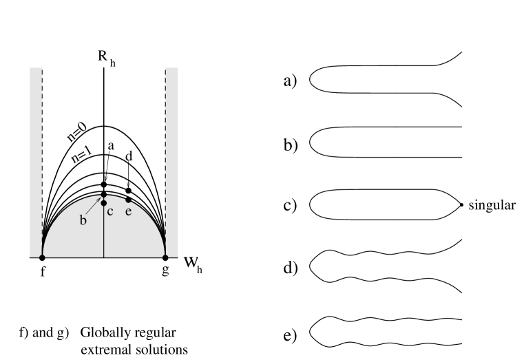
In section 4 we shall study the extremal (or “zero-temperature”) solutions of this system – solutions which have $SO(3,1)$ Lorentz invariance. They are obtained when a non-extremality parameter $\alpha$ is set equal to zero. We shall first consider a subset of BPS solutions (section 4.1) which solve a first-order system following from a superpotential and preserve ${\cal N}=1$, $D=4$ supersymmetry. The family of these BPS solutions is parametrized by one essential parameter $c$; solutions with generic values of $0\leq c\leq\infty$ are singular non-Abelian backgrounds, while the boundary points of the family corresponding to $c=0$ and $c=\infty$ are, respectively, the regular non-Abelian and singular Abelian solutions of [23, 24]. It is the regular non-Abelian solution that was interpreted in [9] as supergravity dual of ${\cal N}=1$ supersymmetric gauge theory.

Non-BPS (supersymmetry-breaking) extremal solutions will be described in section 4.2. We shall start with two “fixed-point” abelian solutions, one of which has a remarkably simple world-sheet description in terms of special kind of $SU(2)\times SU(2)\over U(1)$ gauged WZW model [33] and thus is expected to be an exact string solution to all orders in $\alpha^{\prime}$. We shall then describe a class of regular non-extremal solutions (depending on one parameter $b$) by analyzing asymptotics at $r=0$ and $r=\infty$ and interpolating between them numerically. Presumably, these solutions may be interpreted as “excited states” of the regular BPS solitonic background, similar to higher excitation modes of BPS monopoles. They may be related to supersymmetry-breaking deformations of ${\cal N}=1$ supersymmetric gauge theory dual to the regular BPS background.

In section 5 we shall turn to non-extremal solutions ($\alpha\not=0$) with regular black hole horizons. We shall determine their short-distance behavior, which depends on the two essential parameters $({\rm R}_{h},w_{h})$, the second of which may be interpreted as the U(1) chiral symmetry breaking parameter. The global form of the solutions is found by numerical integration. We shall then compute the corresponding Hawking temperature as a function of the two horizon parameters. As we will explain, there is a minimal non-zero value of the temperature, $T_{c}=1/4\pi$, which is achieved in the limit of large black holes. For ${\rm R}_{h}<\infty$ one has $T>T_{c}$, and the minimal value of $T$ for a fixed ${\rm R}_{h}$ is achieved for the Abelian solution, suggesting restoration of chiral symmetry on the gauge theory side. The limit $T\to\infty$ will lead to globally regular non-Abelian solutions, which break the chiral symmetry.

In section 6 we compute the energy and free energy of the black holes we have found. Remarkably, of the two-parameter family of black hole solutions, only a discrete series of one-parameter families has finite energy. Non-abelian black holes exist only with energy less than a certain threshold; abelian black holes exist only with energy greater than a different threshold—lower than the first, so that there is a range of energies where both abelian and non-abelian solutions are possible.

In section 7 we shall address the question of chiral symmetry restoration at temperatures higher than the Hagedorn temperature. We compare the free energy of a black hole solution with the free energy of the globally regular BPS solution with the same periodicity in Euclidean time at infinity. The thermodynamic instability of the black holes makes it difficult to discuss Hawking-Page transitions meaningfully; however we describe conditions under which black holes would be expected to form.

Section 8 contains a summary of different solutions we obtained and a discussion of possible application of excited monopole solutions in string cosmology context.

While this paper was in preparation there appeared another discussion [49] of a possible relation between non-extremal NS5 on $S^{2}$ background and issues of little string thermodynamics. There is some overlap with our section 5, to the extent that [49] also reached the conclusion that the specific heat is negative. We also make contact briefly with the analysis of [49] in section 7.

2 Ten-dimensional description of 5-branes on $S^{2}$

We shall study solutions in the following subsector of the type IIB supergravity action:

$$S_{10}=\frac{1}{4}\,\int d^{10}x\,\sqrt{-{\bf g}}\,\left(R-\frac{1}{2}\,(\partial\Phi)^{2}-\frac{1}{12}\,e^{-\Phi}\,H_{3}^{2}-\frac{1}{12}\,e^{\Phi}\,F_{3}^{2}\right)\ .$$ (1)

Here $H_{3}=dB_{2}=\frac{1}{6}\,H_{MNS}\,dx^{M}\wedge dx^{N}\wedge dx^{S}$ and $F_{3}=dC_{2}=\frac{1}{6}\,F_{MNS}\,dx^{M}\wedge dx^{N}\wedge dx^{S}$. The line elements in the Einstein frame (used in the above action) and in the string frame are related by $ds_{10E}^{2}={\rm e}^{-\Phi/2}ds_{10S}^{2}={\bf g}_{MN}dx^{M}dx^{N}$. We shall be studying solutions with either $F_{3}$ or $H_{3}$ being zero, so this is a consistent truncation of the type IIB theory. These two cases, i.e. the NS-NS and R-R backgrounds, are related by $S$-duality: if $({\bf g}_{MN},\Phi,H_{3},F_{3}=0)$ is a solution of the field equations, then interchanging $H_{3}\leftrightarrow F_{3}$ and changing $\Phi\to-\Phi$ gives another solution with the same Einstein-frame metric ${\bf g}_{MN}$ (but the string frame metric changes). In what follows we shall mostly consider the R-R version of the solutions.

We shall be considering 3-brane-type solutions with 1+3 “parallel” directions ($t,{\rm x}^{n}$) and 6 transverse directions $(r,\theta_{1},\phi_{1},\psi,\theta_{2},\phi_{2})$ representing a manifold with topology ${\bf R}\times S^{2}\times S^{3}$ and metric similar to conifold metrics [34, 26]. We shall assume that the metric and matter fields have non-trivial dependence on the radial direction $r$ only, while all angular dependence will be fixed by global symmetries.

Let $(\theta_{1},\phi_{1})$ be the standard coordinates on $S^{2}$, and $(\psi,\theta_{2},\phi_{2})$ be the Euler angles on $S^{3}$. We choose the 1-form basis on $S^{2}$ as $(e_{1},e_{2})$,

$$e_{1}=d\theta_{1},\ \ \ \ \ e_{2}=-\sin\theta_{1}d\phi_{1}\,,\ \ \ \ \ \ e_{3}=-\cos\theta_{1}d\phi_{1}\,,$$ (2)

where $e_{3}$ is the spin connection, and the invariant 1-forms on $S^{3}$ as

$$\epsilon_{1}=\cos\psi d\theta_{2}+\sin\psi\sin\theta_{2}d\phi_{2},\ \epsilon_{2}=-\sin\psi d\theta_{2}+\cos\psi\sin\theta_{2}d\phi_{2},\ \epsilon_{3}=d\psi+\cos\theta_{2}d\phi_{2}\,.$$ (3)

These forms satisfy the Maurer-Cartan equation $d\epsilon_{a}+\frac{1}{2}\,\epsilon_{abc}\,\epsilon_{b}\wedge\epsilon_{c}=0$. Let $r$ be the transverse to the brane radial coordinate, while $t$ and ${\rm x}^{n}$ are the time and three longitudinal coordinates.

We shall consider metrics of the following form

$$ds^{2}_{10E}=-Y_{1}\,dt^{2}+Y_{2}\,d{\rm x}^{n}d{\rm x}^{n}+Y_{3}\,dr^{2}+Y_{4}\,(e_{1}^{2}+e_{2}^{2})+Y_{5}\,(\tilde{\epsilon}_{1}^{2}+\tilde{\epsilon}_{2}^{2})+Y_{6}\,\tilde{\epsilon}_{3}^{2}\,,$$ (4)

where

$$\tilde{\epsilon}_{1}\equiv\epsilon_{1}-Y_{7}\,e_{1},\ \ \ \ \ \ \tilde{\epsilon}_{2}\equiv\epsilon_{2}-Y_{7}\,e_{2},\ \ \ \ \ \ \tilde{\epsilon}_{3}\equiv\epsilon_{3}-e_{3},\ \ \$$ (5)

and $Y_{i}=Y_{i}(r)$ are seven functions of the radial coordinate $r$ only.

Strings in such metric may describe confining gauge theories [5], provided $Y_{1}$ and $Y_{2}$ have finite limit for $r\to 0$. That means one has finite fundamental string tension in the IR limit in dual gauge theory.

In the “extremal” case of $Y_{1}=Y_{2}$ one has Lorentz invariance in 1+3 dimensional part, while non-extremal black-hole type solutions should have $Y_{1}/Y_{2}\not=$const. The regular horizon case should then represent finite temperature gauge theory in a deconfined state.

This general class of metrics includes [25, 26] as special cases all 3-brane-on-conifold metrics recently studied in the literature. For example, the subclass with $Y_{4}=Y_{5},Y_{7}=0$ contains metrics whose transverse 6-space is the standard Ricci-flat conifold, $ds_{6}^{2}=dr^{2}+r^{2}(dM_{5})^{2}$, where the base $M_{5}=T^{1,1}=SU(2)\times SU(2)/U(1)$ has

$$dM_{5}^{2}=\frac{1}{6}(d\theta_{1}^{2}+\sin^{2}\theta_{1}d\phi_{1}^{2})+\frac{1}{6}(d\theta_{2}^{2}+\sin^{2}\theta_{2}d\phi_{2}^{2})+\frac{1}{9}(d\psi+\cos\theta_{1}d\phi_{1}+\cos\theta_{2}d\phi_{2})^{2}\ .$$ (6)

Resolved conifold corresponds to $Y_{4}\not=Y_{5},Y_{7}=0$, and deformed conifold has $Y_{7}\not=0$.

For $Y_{7}=0$ the metric has additional $U(1)$ symmetry under $\psi\to\psi+\psi_{0}$, which should correspond to chiral symmetry on the gauge field theory side [8, 9]. If $Y_{7}(r)\to 0$ for $r\to\infty$, this may be interpreted as a supergravity manifestation of chiral symmetry restoration in the high energy (UV) limit. As we shall see below, the symmetry under $\psi\to\psi+\psi_{0}$ may be restored also for $Y_{7}=1$ and $Y_{5}=Y_{6}$.

In addition to the metric, we shall make the following ansatz for the closed R-R 3-form $F_{3}$ [25] ($Y^{\prime}\equiv{dY\over dr}$)

$$F_{3}=P\bigg{[}\,\tilde{\epsilon}_{3}\wedge\left\{{\epsilon}_{1}\wedge{\epsilon}_{2}+{e}_{1}\wedge{e}_{2}-Y_{8}({\epsilon}_{1}\wedge{e}_{2}-{\epsilon}_{2}\wedge{e}_{1})\right\}$$

$$+\ \,Y^{\prime}_{8}dr\wedge({\epsilon}_{1}\wedge{e}_{1}+{\epsilon}_{2}\wedge{e}_{2})\bigg{]}\,,$$ (7)

or, in terms of $\tilde{\epsilon}_{1},\tilde{\epsilon}_{2}$,

$$F_{3}=P\bigg{[}\,\tilde{\epsilon}_{3}\wedge\left\{\tilde{\epsilon}_{1}\wedge\tilde{\epsilon}_{2}+(Y_{7}^{2}-2Y_{7}Y_{8}+1){e}_{1}\wedge{e}_{2}+(Y_{7}-Y_{8})(\tilde{\epsilon}_{1}\wedge{e}_{2}-\tilde{\epsilon}_{2}\wedge{e}_{1})\right\}$$

$$+\ \,Y^{\prime}_{8}dr\wedge(\tilde{\epsilon}_{1}\wedge{e}_{1}+\tilde{\epsilon}_{2}\wedge{e}_{2})\bigg{]}\,.$$ (8)

Here $P$ is a constant which may be interpreted as a charge of D5-brane wrapped on $S^{2}$. Note that $dF_{3}=0$ for any function $Y_{8}=Y_{8}(r)$. Finally, we shall assume that the dilaton may be also non-constant: $\Phi\equiv Y_{9}(r)$.

The global symmetries of our background allow one to derive all supergravity equations from a single 1-d effective action for functions $Y_{i}$. Inserting the above ansatz for the metric and the matter fields into the action (1), integrating over all coordinates except $r$ and dropping the surface term (and the overall volume factor) gives the effective one-dimensional action $S_{1}=\int dr\ L$, where

$$L=\sum_{i,k}G_{ik}(Y)Y_{i}^{\prime}Y_{k}^{\prime}-U(Y)\equiv T-U.$$ (9)

The action has the residual reparametrization invariance $r\to\tilde{r}(r)$ unbroken by our ansatz. Expressing the $Y_{i}$’s in terms of 9 other functions $x,y,z,l,q,p,w,\tilde{w},\Phi$

$$Y_{1}={\rm e}^{2z-6x},\ \ \ \ \ Y_{2}={\rm e}^{2z+2x},\ \ \ \ \ Y_{3}={\rm e}^{10y-2z+2l},\ \$$

$$Y_{4}={\rm e}^{2y-2z+2p+2q},\ \ \ \ Y_{5}={\rm e}^{2y-2z+2p-2q},\ \ \ \ Y_{6}={\rm e}^{2y-2z-8p},$$

$$Y_{7}=w,\ \ \ \ \ \ \ Y_{8}=\tilde{w},\ \ \ \ \ \ \ Y_{9}=\Phi,$$ (10)

to make $G_{ik}$ diagonal, one finds (equivalent action was given in [25])

$$T = {\rm e}^{-l}\left(5y^{\prime 2}-3x^{\prime 2}-2z^{\prime 2}-5p^{\prime 2}-q^{\prime 2}-\frac{1}{4}\,{\rm e}^{-4q}w^{\prime 2}-\frac{1}{4}P^{2}\,{\rm e}^{\Phi+4z-4y-4p}\tilde{w}^{\prime 2}-\frac{1}{8}\Phi^{\prime 2}\right)\,,$$

$$U = \frac{1}{8}\,{\rm e}^{l}\bigg{[}{\rm e}^{8y}\left\{{\rm e}^{-12p}\,[{\rm e}^{4q}+{\rm e}^{-4q}(w^{2}-1)^{2}+2w^{2}(1-{\rm e}^{10p-2q})^{2}]-8{\rm e}^{-2p}\cosh\ 2q\right\}$$ (11)

$$\ \ \ \ \ \ +\ {P^{2}}\,{\rm e}^{\Phi+4z+4y+4p}\left\{{\rm e}^{4q}+{\rm e}^{-4q}(w^{2}-2w\tilde{w}+1)^{2}+2(w-\tilde{w})^{2}\right\}\bigg{]}.$$

Here $l$, which has no kinetic term, is a pure gauge degree of freedom reflecting remaining reparametrization invariance (${\rm e}^{l}$ plays the role of an einbein). Varying with respect to $l$ one can then set it to any value as a reparametrization gauge. In the gauge

$$l=0\ ,$$

the equation of motion for $l$ takes the form of the “zero-energy” constraint $T+U=0$. Another variable with a simple equation of motion is the function $x(r)$: it is a “modulus” of the 1-d action as it does not enter the potential. In the gauge $l=0$ we get

$$x^{\prime\prime}=0,\ \ \ \ \ \ {\rm i.e.}\ \ \ \ \ x=-\frac{1}{4}\alpha\ r\ ,\ \ \ \ \ \ \alpha={\rm const}\geq 0\ .$$ (12)

The constant $\alpha$ is the “non-extremality” parameter (the choice of its sign is of course a convention): note that $Y_{1}/Y_{2}=e^{-8x}$ so that $\alpha\not=0$ corresponds to breaking of the $SO(1,3)$ Lorentz symmetry in the parallel directions in the 10-d metric.

As is clear from the action (1),(11), the charge $P$ can be absorbed into a constant part of the dilaton, and so we shall assume below that $P=1$.

We shall be interested in the special subclass of solutions with

$$w=\tilde{w}\ ,$$

which corresponds to the class of solutions including that of [23, 24, 9]. The consistency with the other equations then requires that

$$q=5p\ ,\ \ \ \ \ \ \ \ \ \Phi+4z-4y+16p=0\ ,$$

in which case the equation of motion for $z$ can be integrated to give

$$z=\frac{1}{2}y-2p+\frac{1}{4}\gamma r\ ,\ \ \ \ {\rm i.e.}\ \ \ \ z=\frac{1}{4}\Phi+\frac{1}{2}\gamma r\ ,\ \ \ \ \ \ \ \gamma={\rm const}\ ,$$

where $\gamma$ is another integration constant.

The functions in the “parallel” part of the metric are then

$$Y_{1}=\exp[\frac{1}{2}\,\Phi+(\gamma+\frac{3}{2}\alpha)r]\ ,\ \ \ \ \ Y_{2}=\exp[\frac{1}{2}\,\Phi+(\gamma-\frac{1}{2}\alpha)r]\ .$$

Assuming that $\gamma+\frac{3}{2}\alpha>0$, the point $r=-\infty$ is the event horizon (as we will see below, $\Phi$ is finite at the horizon). To have regular horizon, we must require that the scale of the flat 3-space factor $Y_{2}$ is finite at the horizon. This gives the condition

$$\gamma=\frac{1}{2}\,\alpha\ .$$

Introducing finally

$$s\equiv 2y+2p\ ,\ \ \ \ \ \ \ \ \ g\equiv 2q=10p\ ,$$

the metric becomes

$$ds_{10E}^{2}={\rm e}^{\Phi/2}\left[-{\rm e}^{2\alpha r}dt^{2}+d{\rm x}^{n}d{\rm x}^{n}+{\rm e}^{4s}dr^{2}+{\rm e}^{2g}(e_{1}^{2}+e_{2}^{2})+\tilde{\epsilon}_{1}^{2}+\tilde{\epsilon}_{2}^{2}+\tilde{\epsilon}_{3}^{2}\right]\,,$$ (13)

where

$$\Phi=s-g-\frac{1}{2}\alpha\ r\ ,$$

while the 3-form is given by (2) with $Y_{7}=Y_{8}=\tilde{w}=w$.

We are finally left with only three independent functions $s$, $g$, and $w$, whose dynamics is determined by the Lagrangian

$$\hat{L}=s^{\prime 2}-\frac{1}{2}\,g^{\prime 2}-\frac{1}{2}\,{\rm e}^{-2g}w^{\prime 2}-\frac{1}{4}{\rm e}^{4s}\left[{\rm e}^{-4g}(w^{2}-1)^{2}-2{\rm e}^{-2g}-1\right]\equiv\hat{T}-\hat{U}\,.$$ (14)

The only effect of the integration constant $\alpha$ is to modify the zero-energy constraint,

$$\hat{T}+\hat{U}=\frac{1}{4}\alpha^{2}\ .$$ (15)

3 $D=4$ description: non-Abelian black holes
in gauged ${\cal N}=4$ supergravity

Before we proceed to analyzing the equations of motion for the Lagrangian (14), let us re-derive these equations using the $D=4$ approach. This is motivated by the fact that the solution of [23, 24, 9] was originally obtained in the context of the $D=4$ supergravity [23], and then was uplifted to $D=10$ [24]. It turns out that the subclass of $D=10$ solutions determined by (13), (14) can be obtained in a similar way – by uplifting the $D=4$ solutions. It will be convenient in what follows to use both the $D=10$ and $D=4$ descriptions, and we shall now establish the precise correspondence between the two.

Let us consider the bosonic part of the action of the four-dimensional ${\cal N}=4$ half-gauged SU(2)$\times$[U(1)]³ supergravity of Freedman and Schwarz (FS) [40]:

$$S_{4}=\int d^{4}x\,\sqrt{-{\bf g}}\,\left(\frac{1}{4}\,R\right. - \frac{1}{2}\,\partial_{\mu}\Phi\,\partial^{\mu}\Phi-\frac{1}{2}\,{\rm e}^{-4\Phi}\,\partial_{\mu}{\bf a}\,\partial^{\mu}{\bf a}$$ (16)

$$- \frac{1}{8}\,{\rm e}^{2\Phi}{\rm F}^{a}_{\ \,\mu\nu}{\rm F}^{a\mu\nu}-\left.\frac{1}{4}\,{\bf a}\ast\!{\rm F}^{a}_{\ \,\mu\nu}{\rm F}^{a\mu\nu}+\frac{1}{4}\,{\rm e}^{-2\Phi}\right)\,.$$

Apart from the gravitational field ${\bf g}_{\mu\nu}$, the model contains the axion ${\bf a}$, the dilaton $\Phi$, and the non-Abelian SU(2) gauge field $A^{a}_{\mu}$ with ${\rm F}^{a}_{\ \mu\nu}=\partial_{\mu}A^{a}_{\nu}-\partial_{\nu}A^{a}_{\mu}+\varepsilon_{abc}A^{b}_{\mu}A^{c}_{\nu}$. The dual field tensor is $\ast\!{\rm F}^{a}_{\mu\nu}=\frac{1}{2}\sqrt{-{\bf g}}\varepsilon_{\mu\nu\lambda\rho}{\rm F}^{a\lambda\rho}$, where $\varepsilon^{0123}=1$. As was shown in [24], this model can be obtained via dimensional reduction of the $D=10$ supergravity (${\cal N}=1$ truncation of (1)) on $S^{3}\times T^{3}$ (the normalizations of the kinetic terms agree after taking into account that the radius of the internal manifold is $\Phi$-dependent). As a result, any on-shell configuration in the FS model, $({\bf g}_{\mu\nu},A^{a}_{\mu},\Phi,{\bf a})$, can be uplifted to $D=10$ to become a solution of ten-dimensional equations of motion for the action (1). The uplifted fields are obtained as follows. The $D=10$ metric in the Einstein frame is given by

$$d{s}^{2}_{10E}={\rm e}^{\Phi/2}\left({\rm e}^{-2\,\Phi}{\bf g}_{\mu\nu}dx^{\mu}dx^{\nu}+\Theta^{a}\Theta^{a}+d{\rm x}^{n}d{\rm x}^{n}\right)\,,$$ (17)

where ($a,b,c=1,2,3$)

$$\Theta^{a}\equiv\epsilon^{a}-A^{a}\ ,\ \ \ \ \ \ \ \ A^{a}=A^{a}_{\mu}dx^{\mu}$$

while $\epsilon^{a}$ are the invariant 1-forms on $S^{3}$. The R-R 3-form is given by

$$F_{3}=\Theta^{1}\wedge\Theta^{2}\wedge\Theta^{3}-\Theta^{a}\wedge{\rm F}^{a}-2{\rm e}^{4\Phi}\ast\!d{\bf a}\,,$$ (18)

Here ${\rm F}^{a}=\frac{1}{2}\,{\rm F}^{a}_{\mu\nu}dx^{\mu}\wedge dx^{\nu}$, and the asterisk stands for the four-dimensional Hodge dual, $\ast(d{\bf a})=\frac{1}{6}\sqrt{-{\bf g}}\,\varepsilon_{\mu\nu\rho\delta}\,\partial^{\mu}{\bf a}\,dx^{\nu}\wedge dx^{\rho}\wedge dx^{\delta}$, while $H_{3}=0$. The $D=10$ dilaton is given by $\Phi+\ln 4$. If the four-dimensional configuration is supersymmetric, then its $D=10$ analog preserves the same amount of supersymmetry.

This correspondence between $D=4$ and $D=10$ backgrounds may be useful for constructing solutions in $D=10$, provided one has some insight into how to solve the 4-dimensional problem. In general, however, it is not easy to solve the equations for the action (16), unless some simplifying assumptions are made. Let us assume that $\partial/\partial x^{0}$ is the hypersurface-orthogonal Killing vector. In this case the most general 4-metric can be represented as

$$ds^{2}_{4}={\bf g}_{\mu\nu}dx^{\mu}dx^{\nu}=-{\rm e}^{2\Phi+2X}dt^{2}+{\rm e}^{2\Phi-2X}h_{ik}(x)\,dx^{i}dx^{k}\,.$$ (19)

We shall also assume that temporal component of the gauge field vanishes, $A_{0}=0$. This implies that the field is purely magnetic, so that $\ast\!{\rm F}^{a}_{\ \,\mu\nu}{\rm F}^{a\mu\nu}=0$, and one can therefore consistently set the axion to zero. We are now left with the 3-metric $h_{ik}$, the gauge field $A^{a}_{i}$, and two scalars $X$ and $\Phi$. The equations of motion for (16) imply that $X$ is a harmonic function,

$$\tilde{\nabla}_{i}\tilde{\nabla}^{i}X=0,$$ (20)

where $\tilde{\nabla}_{i}\tilde{\nabla}^{i}$ is the covariant Laplacian with respect to the 3-metric ${\rm e}^{-2X}h_{ik}$. Since a harmonic function is necessarily unbounded, solutions with non-constant $X$ are singular, or possibly have event horizons. Using (17),(18), any on-shell configuration $(h_{ik},A^{a}_{i},\Phi,X)$ gives rise to the solution in $D=10$:

$$d{s}^{2}_{10E} = {\rm e}^{\Phi/2}\left[-{\rm e}^{2X}dt^{2}+d{\rm x}^{n}d{\rm x}^{n}+{\rm e}^{-2X}h_{ik}dx^{i}dx^{k}+\Theta^{a}\Theta^{a}\right]\,,$$

$$F_{3} = \Theta^{1}\wedge\Theta^{2}\wedge\Theta^{3}-\Theta^{a}\wedge{\rm F}^{a}\,.$$ (21)

Although this could, in principle, give new solutions in $D=10$, the equations of motion for the general static fields $(h_{ik},A^{a}_{i},\phi,X)$ are still rather complicated.

For this reason we now make a further simplifying assumption by demanding that the $D=4$ system is spherically symmetric. In this case the most general 4-metric can be chosen in the form

$$ds^{2}_{4}={\rm e}^{2\Phi}\left[-{\rm e}^{2X}dt^{2}+{\rm e}^{-2X+2\lambda}dr^{2}+{\rm e}^{2g}(d\theta^{2}+\sin^{2}\theta\,d\phi^{2})\right],$$ (22)

where $\Phi$, $X$, $\lambda$, $g$ are functions of the radial coordinate $r$. The components $A^{a}$ of the spherically symmetric, purely magnetic gauge field can be read off from

$$\mbox{\bf T}_{a}A^{a}=w\ (\mbox{\bf T}_{1}\,d\theta-\mbox{\bf T}_{2}\,\sin\theta\,d\phi)-\mbox{\bf T}_{3}\,\cos\theta\,d\phi.$$ (23)

Here $w=w(r)$ and $\mbox{\bf T}_{a}=\frac{1}{2}\tau_{a}$ are constant SU(2) generators ($\tau_{a}$ being Pauli matrices). The corresponding gauge field tensor is

$$\mbox{\bf T}_{a}{\rm F}^{a}=dw\wedge(\mbox{\bf T}_{1}d\theta-\mbox{\bf T}_{2}\sin\theta d\phi)-\mbox{\bf T}_{3}(w^{2}-1)\sin\theta d\theta\wedge d\phi\,.$$ (24)

If $w(r)=0$ then the gauge field is of the Abelian Dirac magnetic monopole type. If $w(r)=\pm 1$, then ${\rm F}^{a}=0$, which implies that the gauge field $A^{a}$ is pure gauge and, therefore, can be gauged away. Below we shall use the fact that the choice $w=\pm 1$ corresponds, in fact, to the vanishing gauge field.

In order to derive the 4d equations of motion, it is convenient to redefine the variables as

$$\lambda=X+2s+l,~{}~{}~{}~{}~{}~{}~{}~{}~{}~{}~{}~{}~{}\Phi=s-g-\frac{1}{2}\,X\,.$$ (25)

Since $X$ is a harmonic function, its equation of motion is

$$(X^{\prime}{\rm e}^{-l})^{\prime}=0\,,$$ (26)

which gives

$$X=X_{0}+\alpha\int{\rm e}^{l}dr\,,$$ (27)

where $X_{0}$ and $\alpha$ are integration constants. Inserting the ansatz (22), (23) into the action (16), integrating and dropping the surface term, the result is $S=4\pi\int dt\int drL$, where (cf. (14))

$$L={\rm e}^{-l}\left(s^{\prime 2}-\frac{1}{2}\,{\rm e}^{-2g}w^{\prime 2}-\frac{1}{2}\,g^{\prime 2}\right)-\frac{1}{4}\,{\rm e}^{4s+l}\left[{\rm e}^{-4g}(w^{2}-1)^{2}-2{\rm e}^{-2g}-1\right]+\frac{1}{4}\alpha^{2}\,{\rm e}^{l}.$$ (28)

Varying this effective Lagrangian gives the system of radial equations

$$({\rm e}^{-l}s^{\prime})^{\prime} = \frac{1}{2}\,{\rm e}^{4s+l}\left(-{\rm e}^{-4g}(w^{2}-1)^{2}+2{\rm e}^{-2g}+1\right),$$ (29)

$$({\rm e}^{-l-2g}w^{\prime})^{\prime} = {\rm e}^{4s-4g+l}(w^{2}-1)w,$$ (30)

$$({\rm e}^{-l}g^{\prime})^{\prime} = {\rm e}^{4s+l}\left(-{\rm e}^{-4g}(w^{2}-1)^{2}+{\rm e}^{-2g}\right),$$ (31)

$$-4s^{\prime 2}+2{\rm e}^{-2g}w^{\prime 2}+2g^{\prime 2} = {\rm e}^{4s+2l}\left({\rm e}^{-4g}(w^{2}-1)^{2}-2{\rm e}^{-2g}-1\right)-\alpha^{2}{\rm e}^{2l},$$ (32)

$$X^{\prime} = \alpha{\rm e}^{l}\,.$$ (33)

The same radial equations can be obtained by inserting the ansatz (22), (23) into the general equations for the action (16). Notice that the integration constant $\alpha$ enters only the last two equations. Since the equations are invariant under $l\to l+l_{0}$, $s\to s-l_{0}/2$, $\alpha\to\alpha{\rm e}^{-\l_{0}}$, the actual value of $\alpha$ is irrelevant, what matters is whether $\alpha$ vanishes or not. Eq.(32), which is the “zero energy condition,” is in fact the initial value constraint. It is sufficient to impose it on the initial (boundary) values of solutions of the independent equations (29)–(31). The constraint generates reparameterizations $r\to\tilde{r}(r)$, which is the residual gauge freedom of the ansatz (22), (23). One can fix the gauge by imposing a gauge condition on the fields $(s,l,g,w)$. For example, one can impose the gauge condition $l=0$, in which case the equation for $X$ can be integrated, $X=X_{0}+\alpha r$.

In the $l=0$ gauge the Lagrangian (28) coincides with the one (14) obtained within $D=10$ approach. Let us also compare the uplifted fields with those given by Eqs.(2),(13) (identifying $\theta=\theta_{1},\ \phi=\phi_{1}$). Using the notation of Eq.(2) one has $A^{1}=we_{1}$, $A^{2}=we_{2}$, $A^{3}=e_{3}$, also ${\rm F}^{1}=dw\wedge e_{1}$, ${\rm F}^{2}=dw\wedge e_{2}$, ${\rm F}^{3}=(w^{2}-1)e_{1}\wedge e_{2}$. The 1-forms $\Theta^{a}$ are then the same as $\tilde{\epsilon}_{a}$ in (5):

$$\Theta^{1}=\tilde{\epsilon}_{1}=\epsilon_{1}-w\,e_{1},\ \ \ \Theta^{2}=\tilde{\epsilon}_{2}=\epsilon_{2}-w\,e_{2},\ \ \ \ \Theta^{3}=\tilde{\epsilon}_{3}=\epsilon_{3}-e_{3}.$$

Then the metric (3) takes the form

$$d{s}^{2}_{10E} = {\rm e}^{\Phi/2}\left[-{\rm e}^{2X}dt^{2}+d{\rm x}^{n}d{\rm x}^{n}+{\rm e}^{4s+2l}dr^{2}+{\rm e}^{2g}(d\theta^{2}+\sin^{2}\theta\,d\varphi^{2})+\tilde{\epsilon}_{c}\tilde{\epsilon}_{c}\right]\,,$$

$$F_{3} = \,\tilde{\epsilon}_{3}\wedge\left[\tilde{\epsilon}_{1}\wedge\tilde{\epsilon}_{2}+(1-w^{2}){e}_{1}\wedge{e}_{2}\right]+\,w^{\prime}dr\wedge({\epsilon}_{1}\wedge{e}_{1}+{\epsilon}_{2}\wedge{e}_{2})\,.$$ (34)

Setting again $l=0$, in which case $X=\alpha r$ (with $X_{0}=0$), these expressions are exactly the same as in (2), (13).

Summarizing, the four-dimensional solutions in the static, spherically symmetric, purely magnetic sector of the half-gauged FS model are equivalent to the “3-brane” backgrounds of Eqs.(2),(13). In what follows we shall study solutions for gravitating Yang-Mills fields in four dimensions described by Eqs.(29)–(33), using (3) in order to construct their ten-dimensional 3-brane analogs.

Before starting to solve the equations of motion, let us rewrite them in another gauge, i.e. choice of the radial coordinate $r$. While the gauge $l=0$ is sometimes useful, in this gauge a finite vicinity of $r=0$ is mapped into an infinite region at spatial infinity, which may cause difficulties in numerical analysis. For that reason, we shall often use instead the gauge where

$$\lambda=0\ ,\ \ \ \ \ \ {\rm i.e.}\ \ \ \ \ \ l=-2s-X\ .$$ (35)

Introducing the functions

$$\nu\equiv{\rm e}^{2X}\ ,\ \ \ \ \ \ \ \ {\rm R}\equiv{\rm e}^{g},$$

the metric becomes

$$ds^{2}_{4}={\rm e}^{2\Phi}(-\nu\,dt^{2}+\nu^{-1}{dr^{2}}+{\rm R}^{2}d\Omega^{2}).$$ (36)

Introducing also another function

$$Z\equiv\Phi^{\prime}\ ,$$

the equations (29)–(33) take the following form in this gauge

$${\rm R}^{\prime\prime}+\frac{3w^{\prime 2}-{\rm R}^{\prime 2}}{{\rm R}}+\frac{{\rm R}^{2}+1}{\nu{\rm R}}-\frac{\nu^{\prime}}{\nu}({\rm R}^{\prime}+2{\rm R}Z)-4{\rm R}Z^{2}-6Z{\rm R}^{\prime}=0\ ,$$ (37)

$$Z^{\prime}+4Z^{2}+\frac{{\rm R}^{\prime 2}-2w^{\prime 2}}{{\rm R}^{2}}-\frac{{\rm R}^{2}+1}{\nu{\rm R}^{2}}+\frac{\nu^{\prime}}{{\rm R}\nu}({\rm R}^{\prime}+2Z{\rm R})+6\frac{Z{\rm R}^{\prime}}{{\rm R}}=0\ ,$$ (38)

$$w^{\prime\prime}+(2Z+\frac{\nu^{\prime}}{\nu})w^{\prime}-\frac{(w^{2}-1)w}{\nu{\rm R}^{2}}=0\ ,$$ (39)

$$2{\rm R}^{2}Z^{2}+4{\rm R}Z{\rm R}^{\prime}+{\rm R}^{\prime 2}+{\rm R}\frac{\nu^{\prime}}{\nu}({\rm R}^{\prime}+{\rm R}Z)-w^{\prime 2}+\frac{(w^{2}-1)^{2}}{2\nu{\rm R}^{2}}-\frac{{\rm R}^{4}+2{\rm R}^{2}}{2\nu{\rm R}^{2}}=0\ ,$$ (40)

$$\nu^{\prime}-\frac{2\alpha}{{\rm R}^{2}}\,{\rm e}^{-2\Phi}=0\ ,$$ (41)

$$\Phi^{\prime}-Z=0\ .$$ (42)

The transformation (with constant $d$)

$$r\to{\rm e}^{2d}r,\ \ \ \Phi\to\Phi+d,\ \ \ \nu\to{\rm e}^{-4d}\,\nu,\ \ \ w\to w,\ \ \ {\rm R}\to{\rm R},\ \ \ Z\to{\rm e}^{2d}Z,\ \ \$$ (43)

maps one solution $\{w(r),\Phi(r),{\rm R}(r),\nu(r)\}$ into another solution $\{w({\rm e}^{2d}r),\Phi({\rm e}^{2d}r)+d,{\rm R}({\rm e}^{2d}r),{\rm e}^{-4d}\nu({\rm e}^{2d}r)\}$. Note that in this gauge the constant $\alpha^{2}$ term is absent in the constraint (40) but is present instead in the equation for $\nu$ in (41).

Another obvious symmetry of the equations is ($C$=const)

$$\Phi\to\Phi+C\ ,\ \ \ \ \ \ \ \ \alpha\to{\rm e}^{2C}\alpha\,,$$ (44)

with all other functions remaining unchanged. Since $\alpha$ appears only in combination with ${\rm e}^{-2\Phi}$, it can be set, when it is non-zero, to some fixed value by a constant shift of $\Phi$.

Finally, there is the symmetry with respect to translations, when argument of all functions is replaced as

$$r\to r+r_{0}\,.$$ (45)

4 Extremal solutions

Let us now study solutions of the above system of equations. There are two distinct cases: $\alpha=0$ and $\alpha\neq 0$, where $\alpha$ is the integration constant in (12) or (33). In the first, “extremal,” case

$$\alpha=0\ ,$$

the $D=10$ metric has $SO(1,3)$ Lorentz symmetry in the 3-brane directions. In the $D=4$ description one has $X^{\prime}=0$, so that $\nu={\rm e}^{2X}={\rm const}$. In view of the scaling symmetry (43) (or simply rescaling $t$ and $r$) one can assume, without loss of generality, that $\nu=1$. Then the $D=4$ metric (36) becomes

$$ds^{2}_{4}={\rm e}^{2\Phi}(-dt^{2}+dr^{2}+{\rm R}^{2}d\Omega^{2}).$$ (46)

Written in the string frame, i.e. without the ${\rm e}^{2\Phi}$ factor, the $t-r$ part of the metric is thus flat. The resulting solutions are either globally regular (i.e. geodesically-complete) or have naked singularities. There is a special subset of BPS solutions preserving part of supersymmetry.

For $\alpha\neq 0$ the 4-d metric function $\nu={\rm e}^{2X}$ is non-trivial, and we get black-hole type solutions that may have a (regular) event horizon. Such finite temperature solutions will be considered in the next section.

4.1 BPS solutions

The system of second-order equations following from (14), (15) or (28) in the case of $\alpha=0$ admits a special subset of solutions which satisfy the first-order system of equations, following from a superpotential $W$. As in many other similar cases, such BPS solutions preserve part of supersymmetry (see, e.g., [41]).

In fact, in the present case, the corresponding first-order system was originally derived in [23] from the conditions for unbroken supersymmetry, i.e. for the existence of non-trivial Killing spinors. In [25] the same system was obtained by first finding the superpotential for the action (14). Since the existence of residual supersymmetry was already checked in [23] (with independent arguments given also in [9, 25]) below we shall follow this more transparent superpotential approach.

Let us write the Lagrangian (28) with $\alpha=0$ in the form (9)

$$L=G_{ik}(y){dy^{i}\over dr}{dy^{k}\over dr}-U(y)\ ,\ \ \ \ \ \ \ \ \ \ \ y^{i}=(s,w,g)\ ,$$ (47)

where $G_{ik}={\rm e}^{-l}{\rm diag}(1,-\frac{1}{2}{\rm e}^{-2g},-\frac{1}{2})$. Direct inspection shows that the potential $U$ can be represented as

$$U=-G^{ik}\frac{\partial W}{\partial y^{i}}\frac{\partial W}{\partial y^{k}}\,,$$ (48)

where the superpotential $W$ is [25]

$$W=\pm\frac{1}{4}{\rm e}^{2s}\sqrt{{\rm e}^{-4g}(w^{2}-1)^{2}+2{\rm e}^{-2g}\,(w^{2}+1)+1}\,\ .$$ (49)

As a result, the Lagrangian (47) can be written as

$$L=G_{ik}\left({dy^{i}\over dr}-G^{ij}\frac{\partial W}{\partial y^{j}}\right)\left({dy^{k}\over dr}-G^{kn}\frac{\partial W}{\partial y^{n}}\right)+2W^{\prime}\,,$$ (50)

and this, in turn, implies that solutions of the first order equations

$${dy^{i}\over dr}=G^{ik}\frac{\partial W}{\partial y^{k}}\ ,$$ (51)

solve also the second-order system.

Writing down the explicit form of the “Bogomol’nyi equations” (51), one finds that the equations for $g^{\prime}$ and $w^{\prime}$ contain only $g$ and $w$, and thus, taking their ratio, gives one first-order equation $dg\over dw$=$f(g,w)$. Introducing

$$u=w^{2}\ ,\ \ \ \ \ \ \ v={\rm e}^{2g}\ ,$$

this equation reads

$$u(v+u-1)\frac{dv}{du}+(u+1)v+(u-1)^{2}=0.$$ (52)

Remarkably, the substitution [23]

$$(u,v(u))\ \to\ (\rho,\xi(\rho))\ :\ \ \ \ \ \ \ \ u=\rho^{2}{\rm e}^{\xi(\rho)},\ \ \ \ \ \ \ v(u)=-\rho\frac{d\xi(\rho)}{d\rho}-u-1$$ (53)

reduces the problem to the simple Liouville equation

$$\frac{d^{2}\xi(\rho)}{d\rho^{2}}=2{\rm e}^{\xi(\rho)}\,.$$ (54)

As a result, one finds the following analytic form of the general solution of the first-order equations (51): in the gauge (35) (i.e. $l=-2s$) the functions in the gauge field (23) and in the 4-d metric (46) are

$$w(r)=\frac{r+r_{0}}{\sinh(r+r_{0}+c)}\,,\ \ \ \ \ \ \ \ \ \ \ {\rm e}^{2g(r)}=2(r+r_{0})\coth(r+r_{0}+c)-w^{2}(r)-1\,,$$

$$\Phi=s-g\ ,\ \ \ \ \ \ \ \ {\rm e}^{2[\Phi(r)-\Phi_{0}]}={\rm e}^{-g(r)}\sinh(r+r_{0}+c)\,.$$ (55)

Here $r_{0}$, $c$, and $\Phi_{0}$ are the three integration constants for the three equations. Different choices of $\Phi_{0}$ correspond to global rescalings of the solution, while $r_{0}$ can be absorbed by shifting $r\to r-r_{0}$.

The parameter $c$ (which without loss of generality may be assumed to be non-negative) is essential, as different values of $c$ lead to qualitatively different solutions. Setting $c=r_{0}=0$ we obtain the globally regular solution,

$$c=0:\ \ \ \ \ w=\frac{r}{\sinh r}\,,\ \ \ \ {\rm e}^{2g}=2r\coth r-w^{2}-1\,,\ \ \ {\rm e}^{2(\Phi-\Phi_{0})}={\rm e}^{-g}\sinh r\,.$$ (56)

Since $w\not=0$, the corresponding 4-d gauge field (23) is non-Abelian. The $r\to 0$ asymptotics of this solution is

$$w=1-{r^{2}\over 6}+O(r^{3})\ ,\ \ \ \ \ {\rm e}^{2g}=r^{2}-{r^{4}\over 9}+O(r^{6})\ ,\ \ \ \ \ {\rm e}^{2(\Phi-\Phi_{0})}=1+{2r^{2}\over 9}+O(r^{4})\ ,$$ (57)

while the $r\to\infty$ asymptotics is given by eq. (58) below. Since the dilaton (string coupling) grows for $r\to\infty$, for large $r$ (i.e. in the UV) one is to switch [9] from the R-R background (describing the IR region of the dual theory) to the S-dual NS-NS one with the same Einstein-frame metric (3) and the dilaton ${\rm e}^{2(\Phi_{NS}+\Phi_{0})}={{\rm e}^{g}\over\sinh r}\to_{r\to\infty}\sqrt{r}{\rm e}^{-r}$.

For $c\neq 0$ solutions have a curvature singularity at the point, where ${\rm e}^{2g}$ vanishes, and the parameter $r_{0}$ can be chosen so that ${\rm e}^{2g}\geq 0$ for $r\geq 0$. For finite values of $c$ these singular solutions have non-Abelian gauge field, while in the limit $c\to\infty$ we get $w=0$, i.e. the gauge field becomes Abelian,

$$w=0\ ,\ \ \ \ \ \ \ {\rm e}^{2g}=2r\ ,\ \ \ \ \ \ \ {\rm e}^{2(\Phi-\Phi^{\prime}_{0})}=\frac{1}{\sqrt{r}}\,{\rm e}^{r}\ .$$ (58)

We have set $r_{0}=1/2$ and shifted $\Phi_{0}$ by an infinite constant ($-c/2$) to put solution into this form. Note that (58) represents the large $r$ asymptotics of the family of BPS solutions (55).

We conclude that, as $c$ is changed from zero to infinity, the family of BPS solutions connects the regular non-Abelian solution (56) with the Abelian solution (58). All these BPS solutions preserve ${\cal N}=1$, $D=4$ supersymmetry.

4.2 Non-BPS solutions

Let us now consider other solutions of the second-order equations (29)–(33) or (37)–(42) which do not satisfy (51), and thus do not preserve supersymmetry. First note that the “Higgs” form of the potential for the gauge-field function $w$ in (14),(28) implies that the equation (31) for $w$ admits two simple “fixed-point” solutions, $w=\pm 1$, and $w=0$. More general non-BPS solutions will not have a simple analytic form (a standard situation for non-BPS monopoles in gauge theories) and will be analyzed by a combination of short- and long-distance expansions and numerical interpolation.

4.2.1 Vanishing gauge field ($w=\pm 1$)

Let us set $w=\pm 1$. In the $l=-2s$ gauge, the field equations (29)–(33) reduce to

$$s^{\prime\prime}+2s^{\prime 2}-\frac{1}{2}={\rm e}^{-2g}\ ,\ \ \ \ \ \ \ \ \ \ \ g^{\prime\prime}+2s^{\prime}g^{\prime}={\rm e}^{-2g}\ ,$$ (59)

$$-4s^{\prime 2}+2g^{\prime 2}+2{\rm e}^{-2g}+1=0\,.$$

As was explained above, for $w=\pm 1$ the gauge field can be gauged away, $A^{a}=0$. As a result, there is no mixing between the $S^{2}$ and $S^{3}$ angles ($\tilde{\epsilon}_{a}=\epsilon_{a}$) in the uplifted $D=10$ background

$$d{s}^{2}_{10E}={\rm e}^{\Phi/2}\left[-dt^{2}+d{\rm x}^{n}d{\rm x}^{n}+dr^{2}+{\rm e}^{2g}(e_{1}^{2}+e_{2}^{2})+\epsilon_{1}^{2}+\epsilon_{2}^{2}+\epsilon_{3}^{2}\right],\ \ \$$ (60)

$$\Phi=s-g\ ,\ \ \ \ \ \ \ \ \ \ \ F_{3}=\epsilon^{1}\wedge\epsilon^{2}\wedge\epsilon^{3}\ .$$

The compact angular part of this is a direct product of $S^{2}\times S^{3}$, i.e. the symmetry of this solution is enhanced as compared to all other solutions with $w\neq\pm 1$: it is invariant under $SU(2)\times SU(2)\times SU(2)$.

Using the third equation in (59) to eliminate ${\rm e}^{-2g}$ from the first two, and introducing $v=g^{\prime}$ and $u=s^{\prime}$, the system reduces to

$$v^{\prime}=2u^{2}-2uv-v^{2}-\frac{1}{2}\,,\ \ \ \ \ \ \ u^{\prime}=-v^{2}\,,$$ (61)

which gives

$$\frac{dv}{du}=1+\frac{2u}{v}+\frac{1-4u^{2}}{2v^{2}}\,.$$ (62)

The numerical solution of this equation will be described below.

4.2.2 Special Abelian solution ($w=0,\ g=0$) and its NS-NS coset sigma model counterpart

For $w=0$, the gauge field (23) is of the Abelian Dirac magnetic monopole type. For $l=-2s$, $\alpha=0$ the equations (29)–(33) reduce to

$$s^{\prime\prime}+2s^{\prime 2}={\rm e}^{-2g}-\frac{1}{2}\,{\rm e}^{-4g}+\frac{1}{2}\ ,\ \ \ \ \ \ \ \ \ \ g^{\prime\prime}+2s^{\prime}g^{\prime}={\rm e}^{-2g}-{\rm e}^{-4g}\ ,$$ (63)

$$-4s^{\prime 2}+2g^{\prime 2}+2{\rm e}^{-2g}+1-{\rm e}^{-4g}=0\ .$$

This system does not seem to have a simple general solution, but there are two important special solutions.

One special solution is already known – the Abelian BPS configuration (58). There is another simple but non-BPS solution representing background with $g=0$, i.e. with constant radius of $S^{2}$.

Indeed, $g=0$ solves the second equation in (63), and then the resulting solution is

$$w=0,\ \ \ \ \ g=0\ ,\ \ \ \ \ \ s=\frac{r}{\sqrt{2}}+s_{0}\ ,\ \ \ {\rm i.e.}\ \ \ \ \ {\rm R}={\rm e}^{g}=1,\ \ \ \Phi=s-g=\Phi_{0}+\frac{r}{\sqrt{2}}\,.$$ (64)

The 4-geometry (46) is thus the direct product of $R^{2}$ and unit $S^{2}$. This solution will be important in what follows, as it will play the role of an attracting fixed point for a class of globally regular non-BPS solutions.

One may wonder if this non-supersymmetric solution is stable. In fact, the instability of the $w=0,g=0$ solution is suggested by the “Higgs” form of the potential for $w$ in the 1-d action (14),(28). Indeed, using the fact that our background is static, and that the metric has 2-d Lorentz symmetry in the $(t,r)$ plane, it is straightforward to generalize the equations (63) to the case of time $t$ and $r$ dependent perturbations near the solution (64) (note that linear $s$ or linear dilaton provides a spatial friction term):

$$-\partial^{2}_{t}\delta w+\delta w^{\prime\prime}+\sqrt{2}\delta w^{\prime}+\delta w=0,\ \ \ -\partial^{2}_{t}\delta{\rm R}+\delta{\rm R}^{\prime\prime}+\sqrt{2}\delta{\rm R}^{\prime}-2\delta{\rm R}=0,\ \ \ \delta Z=-\delta{\rm R}^{\prime}\,.$$ (65)

$w$ has “tachyonic” mass term, and thus its perturbations may grow with time, just as in the standard $(w^{2}-1)^{2}$ scalar potential case. Ignoring time dependence, the four basic solutions of (65) are

$$\delta w=\exp(-\frac{1\pm i}{\sqrt{2}}\,r)\,,\ \ \ \ \ \ \ \ \delta{\rm R}=\exp(-\frac{1\pm\sqrt{5}}{\sqrt{2}}\,r).$$ (66)

Because of the spatial friction term related to linear dilaton, $\delta w$ tends to zero for large $r$, oscillating infinitely many times as it decreases.

The $D=10$ form of this solution (written in S-dual form with $F_{3}$ replaced by the NS-NS 3-form $H_{3}$) has very simple form: in the the string frame the background is the direct product of flat $R^{1,3}$, radial $r$-direction with linear dilaton, and angular 5-space $M^{5}$ supported by $H_{3}$ flux. Explicitly (restoring the dependence on the 3-form charge $P$ and changing the sign of the dilaton)

$$d{s}^{2}_{10\ {\rm NS-NS}}=P\,\left(-dt^{2}+d{\rm x}^{n}d{\rm x}^{n}+dr^{2}+dM^{2}_{5}\right)\ ,\ \ \ \ \ \ dM^{2}_{5}=e_{1}^{2}+e_{2}^{2}+{\epsilon}_{1}^{2}+{\epsilon}_{2}^{2}+\tilde{\epsilon}_{3}^{2}\,,$$ (67)

$$\Phi_{\rm NS-NS}=-\Phi=-\Phi_{0}-\frac{r}{\sqrt{2}}\ ,\ \ \ \ \ \ \ \ \ \ \ \ H_{3}=P\,\tilde{\epsilon}_{3}\wedge\left({\epsilon}_{1}\wedge{\epsilon}_{2}+{e}_{1}\wedge{e}_{2}\right)\ .$$ (68)

This NS-NS background may be interpreted as a near-throat region of NS5-brane wrapped over the transverse $S^{2}$ in a special way that breaks all supersymmetries. As in other NS5 brane cases (like the regular BPS solution (56), this NS-NS description is valid for $r\gg 0$ when the coupling is small, while for small $r$ one needs to consider the S-dual background [43].

Like the throat region of the standard NS5-brane [42] described by $R^{1,6}\times S^{3}$ or $SU(2)$ WZW model with linear dilaton, this model has a remarkably simple world-sheet conformal sigma model interpretation.

Indeed, the $M^{5}$ metric

$$dM_{5}^{2}=d\theta_{1}^{2}+\sin^{2}\theta_{1}d\phi_{1}^{2}+d\theta_{2}^{2}+\sin^{2}\theta_{2}d\phi_{2}^{2}+(d\psi+\cos\theta_{1}d\phi_{1}+\cos\theta_{2}d\phi_{2})^{2}$$ (69)

is of the same $\frac{SU(2)\times SU(2)}{U(1)}$ coset form as the $T^{1,1}$ metric (6), but now the relative coefficients of the $U(1)$ and $S^{2}$ factors are equal since this is not an Einstein space but rather a solution of the 5-d Einstein equations with the ${H}_{3}$ stress tensor term. We shall call this space $\tilde{T}^{1,1}$.

The 3-form

$$H_{3}=P\,(d\psi+\cos\theta_{1}d\phi_{1}+\cos\theta_{2}d\phi_{2})\wedge(\sin\theta_{2}d\theta_{2}\wedge d\phi_{2}-\sin\theta_{1}d\theta_{1}\wedge d\phi_{1}),$$ (70)

has potential ($H_{3}=dB_{2}$)

$$B_{2}=P\left[(\cos\theta_{1}d\phi_{1}-\cos\theta_{2}d\phi_{2})\wedge d\psi+\cos\theta_{1}\cos\theta_{2}d\phi_{1}\wedge d\phi_{2}\right]\ .$$ (71)

Combining the $\tilde{T}^{1,1}$ metric (69) with this antisymmetric 2-tensor we get the same D=5 NS-NS background that was discovered recently [33] as a simplest representative in a special class of $\frac{G\times G^{\prime}}{H}=\frac{SU(2)\times SU(2)}{U(1)}$ coset sigma models introduced in [44]. As was checked in [33], the corresponding bosonic sigma model is conformally invariant in the one- and two-loop approximation (3-loop approximation in the world-sheet supersymmetric case), and there are good reasons to believe that (in a proper scheme) these backgrounds are exact NS-NS string solutions to all orders in $\alpha^{\prime}$.

The string world-sheet action of this $\frac{SU(2)\times SU(2)}{U(1)}$ coset model is obtained as follows. Let $(\psi_{1},\theta_{1},\phi_{1})$ and $(\psi_{2},\theta_{2},\phi_{2})$ be the Euler angles that parametrize the two SU(2) group manifolds. Taking the sum of the two SU(2) WZW models with equal levels $k=P\in Z$ and adding the current-current interaction term [44] with the same coefficient $P$ one finds [33]

$$I=\frac{P}{4\pi}\int d^{2}\sigma\bigg{[}\partial_{\mu}\theta_{1}\partial^{\mu}\theta_{1}+\partial_{\mu}\phi_{1}\partial^{\mu}\phi_{1}+\partial_{\mu}\psi_{1}\partial^{\mu}\psi_{1}+\cos\theta_{1}\partial_{\mu}\phi_{1}\partial_{\nu}\psi_{1}\,(\eta^{\mu\nu}+\epsilon^{\mu\nu})$$

$$+\ \partial_{\mu}\theta_{2}\partial^{\mu}\theta_{2}+\partial_{\mu}\phi_{2}\partial^{\mu}\phi_{2}+\partial_{\mu}\psi_{2}\partial^{\mu}\psi_{2}+\cos\theta_{2}\partial_{\mu}\phi_{2}\partial_{\nu}\psi_{2}\,(\eta^{\mu\nu}+\epsilon^{\mu\nu})$$

$$+\ (\cos\theta_{1}\partial_{\mu}\phi_{1}+\partial_{\mu}\psi_{1})(\cos\theta_{2}\partial_{\nu}\phi_{2}+\partial_{\nu}\psi_{2})\,(\eta^{\mu\nu}+\epsilon^{\mu\nu})\bigg{]}.$$ (72)

The U(1) gauge invariance of this action allows one to set $\psi_{2}=0$ as a gauge choice. Denoting then $\psi\equiv\psi_{1}$, the coset model (4.2.2) becomes the same as the string sigma model corresponding to the D=5 target space (69),(71).

The exact central charge of (world-sheet supersymmetric version of) this model is

$$c=2\times\frac{3k^{\prime}}{k^{\prime}+2}-1=5-\frac{12}{k}\ ,\ \ \ \ \ \ \ k^{\prime}=k-2\ ,\ \ \ \ ~{}~{}~{}k=P\,.$$ (73)

As in the case of the NS5 throat model, the central charge deficit of this coset model is canceled by the linear dilaton in (68). Indeed, the central charge (dilaton $\beta$-function) equation

$$\bar{\beta}^{\Phi}=\frac{1}{4}\,(D-10)+\alpha^{\prime}\left[-\frac{1}{2}\nabla^{2}\Phi+(\partial\Phi)^{2}-\frac{1}{24}H_{3}^{2}\right]+O(\alpha^{\prime 4})\,$$ (74)

vanishes for the $D=10$ background (67) (here $D=10,\ (\partial\Phi)^{2}={1\over 2}=\frac{1}{24}H_{3}^{2}={1\over 6}R$).

It is possible to check directly (e.g., following the discussion in [25]) that this solution breaks all supersymmetries (all such coset models in [33] were claimed to be non-supersymmetric). It may have a relation to some non-supersymmetric deformation of D=6 little string model compactified on $S^{2}$. Returning back to the S-dual R-R background supported by the 3-form $F_{3}$, one may write down the corresponding string-frame metric as ($g_{s}={\rm e}^{\Phi_{0}}$)

$$ds_{10\ {\rm R-R}}^{2}=g_{s}P{\rm e}^{{1\over\sqrt{2}}r}(-dt^{2}+d{\rm x}^{n}d{\rm x}^{n}+dr^{2}+dM_{5}^{2})\equiv d\rho^{2}+{1\over 2}\rho^{2}(-dt^{2}+d{\rm x}^{n}d{\rm x}^{n}+dM_{5}^{2})\ .$$ (75)

One may speculate that string theory in this simple background may be dual to a non-supersymmetric deformation of ${\cal N}=1$ supersymmetric theory discussed in [9].

This NS-NS (or R-R) solution admits a trivial non-extremal generalization (to be discussed below): one is simply to replace the $(t,r)$ part of the metric and the dilaton by the 2-d dilatonic black hole background [45].

4.2.3 Globally regular solutions

Consider now general extremal non-BPS solutions of the second order field equations with non-constant $w$. For $\alpha=0$ (i.e. $\nu={\rm const}=1$) the independent field equations (37)–(42) reduce to

$${\rm R}^{\prime\prime}+\frac{3w^{\prime 2}-{\rm R}^{\prime 2}+1}{{\rm R}}-4{\rm R}Z^{2}+{\rm R}-6Z{\rm R}^{\prime}=0,$$

$$Z^{\prime}+4Z^{2}+\frac{{\rm R}^{\prime 2}-2w^{\prime 2}-1}{{\rm R}^{2}}+6\frac{Z{\rm R}^{\prime}}{{\rm R}}=1,$$

$$w^{\prime\prime}+2Zw=\frac{(w^{2}-1)w}{{\rm R}^{2}},\ \ \ \ \ \ \ \ Z\equiv\Phi^{\prime}\ ,$$ (76)

plus the constraint

$$2{\rm R}^{2}Z^{2}+4{\rm R}Z{\rm R}^{\prime}+{\rm R}^{\prime 2}-1-w^{\prime 2}+\frac{(w^{2}-1)^{2}}{2{\rm R}^{2}}-\frac{1}{2}{\rm R}^{2}=0.$$ (77)

We will be interested in solutions that are globally regular. This means that either the curvature is everywhere bounded or it takes an infinite geodesic time to reach the region with unbounded curvature – the spacetime manifold is geodesically complete. First of all, we shall consider solutions that have a regular origin, which is the point $r=r_{0}$ where ${\rm R}$ vanishes but the curvature is bounded. One can set $r_{0}=0$. The manifold cannot be analytically continued towards negative $r$ in this case, and so one can assume without loss of generality that $r\geq 0$. The inspection of the field equations shows that such solutions form a one-parameter family, with the following small $r$ Taylor expansion:

$${w=1-br^{2}+O(r^{4}),\ \ \ \ \ \ \ Z=\Phi^{\prime}=2(b^{2}+\frac{1}{12})r+O(r^{3}),} {{\rm R}={\rm e}^{g}=r-(b^{2}+\frac{1}{36})r^{3}+O(r^{5}),\ \ \ \Phi=\Phi(0)+(b^{2}+\frac{1}{12})r^{2}+O(r^{4})\,.}$$ (78)

Here $b$ and $\Phi(0)$ are free parameters. The value

$$b={1\over 6}$$

corresponds to the regular BPS solution (56), while for $b\neq{1\over 6}$ we obtain its regular, non-BPS deformations. Expansions (78) determine only local solutions for small $r$, and the next step is to extend these solutions to finite values of $r$. Our strategy will be to numerically integrate Eqs. (4.2.3) in the interval $r\in[0,\infty)$ using (78) as the boundary conditions at $r=0$. Since the constraint (77) is fulfilled by the initial values (78), it holds for all $r$.

Let us discuss the boundary conditions at $r=\infty$. Having in mind future applications, let us consider the general equations (37)–(42) with $\alpha\neq 0$. Assuming that ${\rm R}\to\infty$ for large $r$, we find the following series solutions in the vicinity of $r=\infty$:

$${\rm R} = \sqrt{2x}-\frac{\Upsilon^{2}}{\sqrt{2}x^{3/2}}\,(1-\frac{1}{4}\cdot\frac{3\Upsilon^{2}-10}{x}+\ldots)+\sqrt{2}{\cal P}x{\rm e}^{-x}(1+\frac{2}{x}+\ldots)+O({\rm e}^{-2x})\,,$$

$$\Phi = \Phi_{\infty}+\frac{x}{2}-\frac{1}{4}\ln x+\frac{5\Upsilon^{2}}{16x^{2}}\,(1-\frac{2}{5}\cdot\frac{2\Upsilon^{2}-7}{x}+\ldots)-{\cal P}\sqrt{x}{\rm e}^{-x}(1+\frac{1}{x}+\ldots)+O({\rm e}^{-2x})\,,$$

$$w = \frac{\Upsilon}{\sqrt{x}}\,(1+\frac{1-\frac{1}{2}\Upsilon^{2}}{x}+\ldots)+{\cal C}x{\rm e}^{-x}(1+\ldots)+O({\rm e}^{-2x})\,,$$

$$\nu = \frac{1}{\mu^{2}}-\frac{\alpha}{\sqrt{x}}\,{\rm e}^{-x-2\Phi_{\infty}}(1+\ldots)+O({\rm e}^{-2x})\,,\ \ \ \ \ \ \ \ \ x\equiv\mu(r+r_{\infty})\ .$$ (79)

Here $\mu$, $r_{\infty}$, ${\cal P}$, $\Phi_{\infty}$, $\Upsilon$, ${\cal C}$ are six integration constants. Notice that 6 is the maximal number of integration constants a solution can have: Eqs.(37)–(42) can be reformulated as a system of 7 first order equations plus one constraint. As a result, (4.2.3) determines asymptotics of a generic solution for which ${\rm R}\to\infty$ for $r\to\infty$. There are also solutions for which ${\rm R}$ is bounded for large $r$. It is worth noting that solutions with asymptotics (4.2.3) are geodesically complete for large $r$, and moreover all curvature invariants determined by (4.2.3) vanish for $r\to\infty$.

The parameter $\mu$ (which may be interpreted as the dilaton charge at infinity) reflects the scaling symmetry (43) of the equations. Comparing with (56), (58), we conclude that for large $r$ the solutions generically have the same asymptotics as the BPS solutions (56), up to a rescaling and a shift, plus the polynomial terms proportional to $\Upsilon$, and plus also the exponentially small terms proportional to ${\cal P}$.

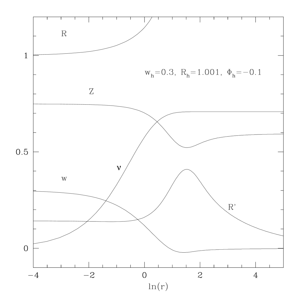
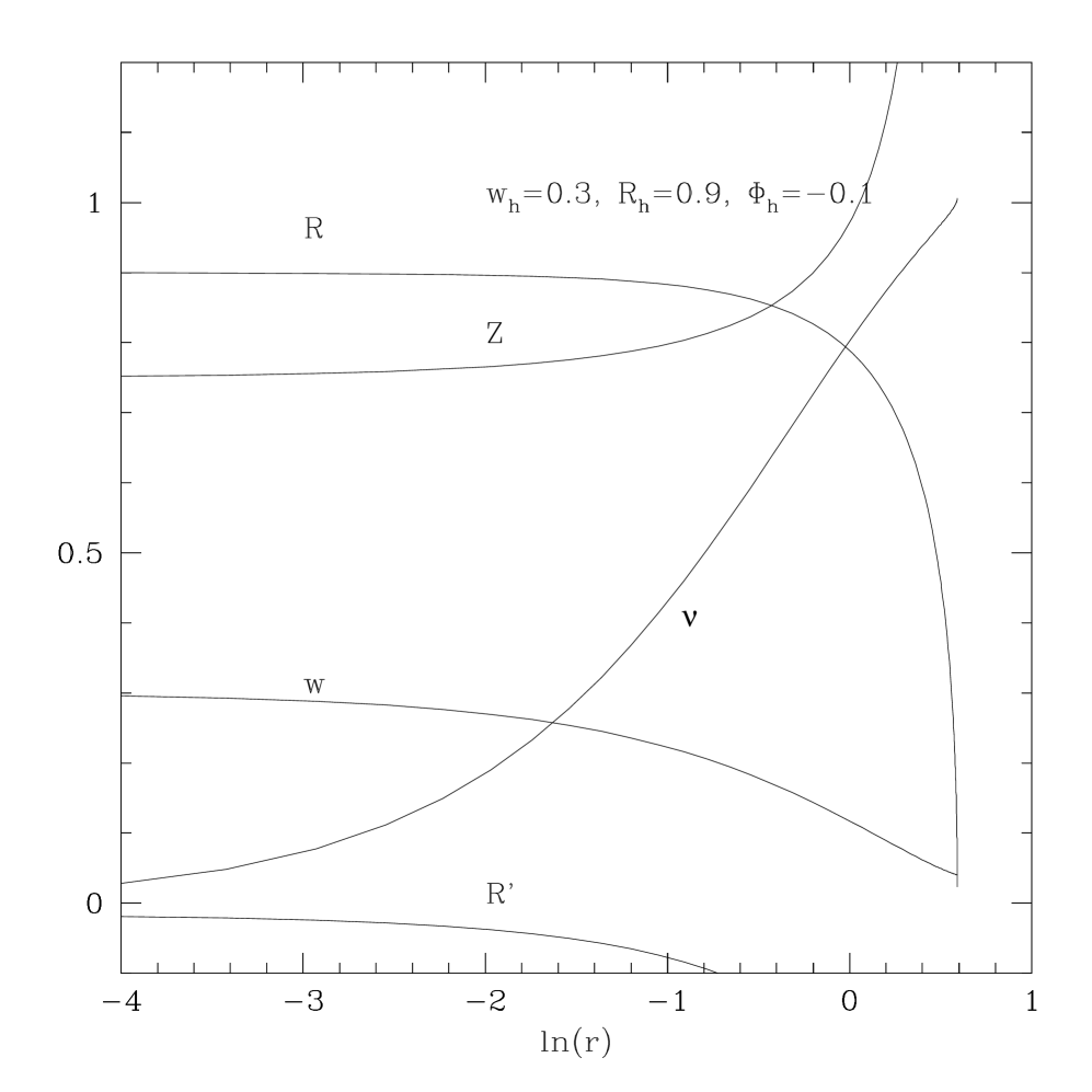
In the extremal case of $\alpha=0$ the solutions for $r\to\infty$ are then given by (4.2.3) with $\mu=1$ (we are assuming $\nu=\nu_{0}=1$). The next step is to numerically interpolate between the $r\to 0$ asymptotics (78) and these large $r$ asymptotics, to find the one-parameter family of regular solutions in the whole interval $[0,\infty)$. It turns out that for any $b\in(0,1/2)$ the local regular solution (78) can be extended all the way up to the infinity to meet the asymptotic solution (4.2.3) with certain special $b$-dependent values of the parameters $\mu(b)$, $r_{\infty}(b)$, ${\cal P}(b)$, $\Phi_{\infty}(b)$, $\Upsilon(b)$, ${\cal C}(b)$ (see Figs.13,15).

Figure 1: Non-BPS solution for $b=0.2$.

Figure 2: Non-BPS solution for $b=0.499$.

The behavior of the solutions is illustrated in Fig.2 and Fig.2. For $0<b<1/6$ the function $w$ is always positive, while for $b>1/6$ it has at least one zero. As $b$ tends to 1/2, $w$ develops more and more oscillations around zero, while the functions ${\rm R}$ and $Z$ start oscillating around their constant values ($1$ and $1/\sqrt{2}$, respectively) corresponding to the special Abelian solution (64). Thus, one may say that the solution (64) acts as the large-$r$ attracting fixed point for these regular solutions. Specifically, among the four independent linear fluctuation modes (66) near this special solution there are three modes that are regular for large $r$. These modes parameterize the “stable manifold” in the vicinity of the fixed point, and their existence is the reason why the nearby phase trajectories approach the fixed point. As a result, the trajectory that starts from the origin gets attracted by the fixed point (66) and stays longer and longer in its vicinity as $b$ tends to 1/2. However, for $b<1/2$, the trajectory finally gets repelled from the fixed point due to the existence of the fourth, unstable, mode in (66), and after that it goes to the region where R is infinite.

4.2.4 Limiting solutions

A very interesting phenomenon occurs for the special case of $b=1/2$. For $b\to 1/2$ the trajectory approaches the fixed point (64) closer and closer, and finally for $b=1/2$ the limiting trajectory splits into two parts. For the first, interior part the trajectory starts from the origin at $r=0$, and in the limit $r\to\infty$ arrives exactly at the fixed point (64) – after infinitely many oscillations. The second, exterior part of the limiting trajectory corresponds to the solution that interpolated between the fixed point (64) and infinity.

Figure 3: Interior limiting solution

Figure 4: Exterior limiting solution

Let us construct first the interior limiting solution. Returning back to the Lagrangian (28), we introduce the new variables $p(r)$, $f(r)$ related to $w(r)$, $g(r)$ via

$$w=\ \cosh p\ \cos f,\ \ \ \ \ \ \ \ \ \ \ {\rm e}^{g}=\ \cosh p\ \sin f\,.$$ (80)

The Lagrangian then becomes

$$L={\rm e}^{-l}\left(s^{\prime 2}-\frac{f^{\prime 2}}{2\sin^{2}f}-\frac{\tanh^{2}p\ \,p^{\prime 2}}{2\sin^{2}f}\right)-\frac{1}{4}\,{\rm e}^{4s+l}\left(\frac{\tanh^{4}p}{\sin^{4}f}-\frac{2}{\sin^{2}f}\right)-\frac{\alpha^{2}}{4}\,{\rm e}^{l}\,.$$ (81)

The advantage of such a parameterization is that, as one can immediately see, $p(r)=0$ is a solution of the equations of motion. This means that the field equations admit the following first integral

$$w^{2}+{\rm e}^{2g}=1\,.$$ (82)

It turns out that for $b=1/2$ this condition arises automatically. Indeed, the equation for $p(r)$ derived from (81) shows that for $b=1/2$ the function $p$ and all its derivatives at $r=0$ vanish. As a result, we have $p=0$, and the Lagrangian (81) becomes simply

$$L={\rm e}^{-l}s^{\prime 2}-\frac{{\rm e}^{-l}f^{\prime 2}}{2\sin^{2}f}+\frac{{\rm e}^{4s+l}}{2\sin^{2}f}\ .$$ (83)

The field equations are then (in the gauge $l=-2s$)

$$s^{\prime\prime}+2s^{\prime 2}=\frac{1}{\sin^{2}f},\ \ \ \ \ f^{\prime\prime}+2s^{\prime}f^{\prime}=\ (1+f^{\prime 2})\cot f\ ,\ \ \ \ \ 2\,s^{\prime 2}\sin^{2}f=f^{\prime 2}+1\,.$$ (84)

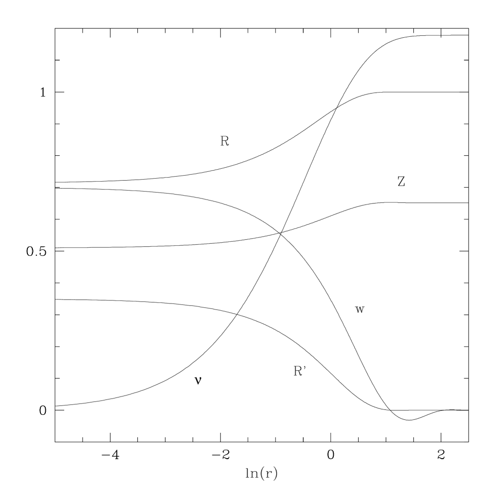
The solution will be regular at the origin if $s=\ln r+O(r^{2})$ and $f=r+O(r^{3})$ for $r\to 0$. Integrating (84) with these boundary conditions shows that $f\to\pi/2$ for large $r$. Reconstructing $w$, ${\rm R}$, and $Z=s^{\prime}-f^{\prime}\cot f,$ finally gives the solution shown in Fig.4. This solution is globally regular (regular at $r=0$) and for large $r$ it tends to the special Abelian solution (64).

Consider now the exterior limiting solution. Here ${\rm R}$ never vanishes, so the range of $r$ is to be taken from $-\infty$ to $+\infty$. The solution starts from the special Abelian solution (64) at $r=-\infty$. Eq.(66) shows that there is only one mode around this solution which is stable for $r=-\infty$: $\delta w=0$, $\delta{\rm R}=\exp(-\frac{1-\sqrt{5}}{\sqrt{2}}\,r)$, $\delta Z=-\delta{\rm R}^{\prime}$. This shows that we must keep $w=0$ for all $r$, while ${\rm R}$, $Z$ can deviate from the values determined by the solution (64), so that for $r\to-\infty$

$${\rm R}=1+\exp(\frac{\sqrt{5}-1}{\sqrt{2}}\,(r-r_{0}))+\ldots\,,\ \ \ \ Z=\frac{1}{\sqrt{2}}+\frac{1-\sqrt{5}}{\sqrt{2}}\exp(\frac{\sqrt{5}-1}{\sqrt{2}}\,(r-r_{0}))+\ldots\,.\ \ \$$ (85)

Here $r_{0}$ is an arbitrary parameter corresponding to the possibility of global translations. Integrating the field equations with such boundary conditions shows that for $r\to+\infty$ the solution follows the asymptotic behavior (4.2.3); see Fig.4.

To recapitulate, both the interior and exterior limiting solutions shown in Fig.4 and Fig.4 are globally regular. The interior solution interpolates in the interval $[0,\infty)$ between the regular origin and the special Abelian solution (64). The exterior solution interpolates for $r\in(-\infty,+\infty)$ between the solution (64) and the asymptotic (BPS) solution (4.2.3).

Summarizing this section, globally regular solutions exist for $b\in[0,1/2]$. The solution with $b=0$ has not been described so far: in this case $w(r)=1$, which corresponds to the case described by Eq.(62). The qualitative behavior of ${\rm R}$ and $Z$ is then similar to that shown in Fig.2. If $b<0$ then solutions are still regular at the origin, but $w$ diverges at some finite $r$, where these solutions develop a curvature singularity. For $b>1/2$ solutions have compact spatial sections, since ${\rm R}$ develops a second zero (in addition to the one at $r=0$) at some finite $r$, where the geometry is singular. This type of behavior is somewhat similar to what is shown in Fig.6 for black holes.

As we shall see below, among all globally regular solutions described above, there is only a discrete subset of solutions for which the energy is finite.

5 Non-Extremal solutions: Black holes

5.1 Solutions with regular horizon

We shall now turn to non-extremal solutions that have a non-constant function $X$ in the 10-d metric (3) or $\nu$ in the 4-d metric (36), corresponding to the case of non-zero non-extremality parameter $\alpha$ in (33) or (41). Such solutions generalize the regular extreme solutions described in the previous section to the case when an event horizon is present. Since $\alpha$ enters (41) in combination $2\alpha e^{-2\Phi}$, it can be rescaled by shifting $\Phi$ by a constant. In particular, one can set $\alpha=1/2$, which we shall assume in our numerical analysis. Since $\nu={\rm e}^{2X}$ is non-constant, such non-extremal solutions may have a regular event horizon. A solution has a regular event horizon if there is a point $r=r_{h}$ where $\nu$ has a simple zero, while all other functions are finite and differentiable at this point.

Without loss of generality one can set $r_{h}=0$ (since the equations are autonomous). The field equations then admit, in the vicinity of $r=0$, local solutions characterized by the following Taylor expansions:

$$\nu=\frac{2\alpha{\rm e}^{-2\Phi_{h}}}{{\rm R}_{h}^{2}}\,r+O(r^{2})\,,\ \ \ \ \ \ \ \ \ \ w=w_{h}+(2\alpha{\rm e}^{-2\Phi_{h}})^{-1}w_{h}(w_{h}^{2}-1)\,r+O(r^{2})\,,$$

$${\rm R}={\rm R}_{h}+(2\alpha{\rm e}^{-2\Phi_{h}})^{-1}\frac{{\rm R}_{h}^{2}-(w_{h}^{2}-1)^{2}}{{\rm R}_{h}}\,r+O(r^{2})\,,$$

$$\Phi=\Phi_{h}+(2\alpha{\rm e}^{-2\Phi_{h}})^{-1}\frac{{\rm R}_{h}^{4}+(w_{h}^{2}-1)^{2}}{2{\rm R}^{2}_{h}}\,r+O(r^{2}).$$ (86)

The parameter $\kappa\equiv 2\alpha e^{-2\Phi_{h}}$ may be interpreted as a characteristic “mass scale” of black hole. The free parameters $\Phi_{h}$, ${\rm R}_{h}$, and $w_{h}$ determine the value of the dilaton at the horizon, the “radius” of the horizon, and the value of $w$ at the horizon. One may check that all curvature invariants are finite at the horizon.

We now numerically integrate Eqs.(37)–(42) towards large $r$ using (86) as initial values at $r=0$. For each set of values of $\Phi_{h}$, $w_{h}$, and ${\rm R}_{h}$ this gives us a black hole solution living in the interval $r\in[0,r_{\ast}]$, where $r_{\ast}$ can be either finite or infinite. The set of black hole solutions is therefore three dimensional and has one dimension more as compared to the regular solutions described in the previous section, where we had only two parameters – $b$ and $\Phi(0)$ in (78). The additional parameter arising in the black hole case determines the radius of the even horizon.

In order to qualitatively describe these black hole solutions for different values of $\Phi_{h}$, $w_{h}$, and ${\rm R}_{h}$, we first notice that choosing different values of $\Phi_{h}$ leads merely to global rescalings of the configurations. For this reason we can set $\Phi_{h}=0$, since for other values of $\Phi_{h}$ the structure of solutions is qualitatively similar.

Figure 5: Black holes with ${\rm R}_{h}>\sqrt{1-w_{h}^{2}}$. This corresponds to Figure 9a.

Figure 6: Black holes with ${\rm R}_{h}<\sqrt{1-w_{h}^{2}}$. This corresponds to Figure 9b.

Since the equations (37)–(42) are symmetric under $w\to-w$, one can assume that $w_{h}\geq 0$, and then one can show that $w_{h}$ must belong to the interval $[0,1]$, since otherwise $w$ diverges at some finite $r$.

Setting $w_{h}=0$, we will obtain Abelian solutions with $w=0$, while $w_{h}\neq 0$ will give non-Abelian solutions. They are qualitatively similar, the only difference is that for Abelian solutions $w=0$ everywhere, while for non-Abelian ones $w$ starts from a finite value at the horizon and then approaches zero for large $r$. As was discussed above, configurations with $w=0$ respect the $U(1)$ symmetry ($\psi\to\psi+\psi_{0}$), so $w_{h}$ may be regarded as an order parameter for chiral symmetry breaking.

The horizon value of ${\rm R}$ – the parameter ${\rm R}_{h}$ plays a crucial role. For ${\rm R}_{h}>\sqrt{1-w_{h}^{2}}$, the solution has the asymptotic form (4.2.3), such that ${\rm R}\to\infty$ for $r\to\infty$. A typical solution of this form is illustrated in Fig.6. For ${\rm R}_{h}<\sqrt{1-w_{h}^{2}}$, the event horizon is still regular, but the asymptotics change completely. ${\rm R}$ is no longer unbounded, but reaches a maximal value at some finite $r$; after that it decreases and finally vanishes at some $r=r_{\ast}$, where there is a curvature singularity. Such a solution is illustrated in Fig.6.

Figure 7: A typical solution with ${\rm R}_{h}=\sqrt{1-w_{h}^{2}}$. The oscillations in $w$ are matched by oscillations in ${\rm R}$, too small to be seen in this figure. These oscillations are depicted in Figure 9d in magnified form.

Figure 8: Non-extremality $\alpha$ for black hole solutions with R${}_{h}>\sqrt{1-w_{h}^{2}}$ normalized such that $\Phi_{h}=0$, $\nu(\infty)=1$. The region above (below) the curves corresponds to values of $\alpha$ for solutions with $\Phi_{h}>0$ ($\Phi_{h}<0$).

In the “intermediate” case, i.e. for ${\rm R}_{h}=\sqrt{1-w_{h}^{2}}$, the function ${\rm R}$ tends, for large $r$, to a constant ${\rm R}_{\infty}$. The whole configuration asymptotically approaches the (rescaled) special Abelian solution (64), so that $w$ oscillates, $w\sim e^{-Z_{\infty}r}\sin(Z_{\infty}(r-r_{0}))$, and $Z-Z_{\infty}\sim{\rm R}-{\rm R}_{\infty}\sim e^{-Z_{\infty}r}$. Such a solution is illustrated in Fig. 8. For $w_{h}=0$ and ${\rm R}_{h}=1$ the solution is easy to find analytically by solving (37)–(42):

$$w=0,\ \ \ \ \ {\rm R}=1,\ \ \ \ \ \ Z={\rm const},\ \ \ \ \Phi=\Phi_{0}+Zr,\ \ \ \ \ \nu=\frac{1}{2Z^{2}}-\frac{\alpha}{Z}\,{\rm e}^{-2\Phi_{0}-2Zr}.$$ (87)

For $\alpha=0$, choosing $Z={1\over\sqrt{2}}$ we get the extremal solution (64). In the case of $\alpha\not=0$ the 4-d metric (36) is simply the direct product of $S^{2}$ and the 2-d dilatonic black hole background (with the “cigar” metric in euclidean signature case) [45].

For $w_{h}\neq 0$ and ${\rm R}_{h}=\sqrt{1-w_{h}^{2}}$ the non-abelian component of the gauge field is turned on, leading to more general solutions which may be thought of as finite deformations of the “cigar”.

Figure 9: A qualitatively correct depiction of the “phase diagram” of black hole solutions, and of particular solutions. Quantitatively correct plots showing some of the same information can be found in Figs.6, 6, 8, 8, 17, and 17. Left: In the unshaded region, solutions are asymptotic to (4.2.3); in the shaded region, solutions are singular at finite $r$; and on the semi-circular border between I and II, solutions are asymptotic to the cigar geometry. The dark lines represent those solutions for which $\Upsilon=0$ in (4.2.3), which means that the asymptotics at infinity is asymptotically close to the BPS solution. Right: The $(t,r)$ parts of the metrics, in Euclidean signature, are the surfaces of revolution of the curves shown.

The results of the previous paragraph were discovered numerically, although it may be possible to prove them directly by qualitative analysis of the system of differential equations. To support the claim that for ${\rm R}_{h}=\sqrt{1-w_{h}^{2}}$ the solution is asymptotic to the cigar geometry for large $r$, recall the parametrization (80). Putting ${\rm R}_{h}=\sqrt{1-w_{h}^{2}}$ amounts to setting the function $p$ in (80) to zero at the horizon, and, as we saw before, this implies $p=0$ everywhere, so that $w^{2}+{\rm R}^{2}=1$. Linearizing the analytic solution (87) around $w=0$, one finds the claimed damped oscillatory behavior, which is actually the same as in Eq.(66), so this solution is a stable attractor as one proceeds to large $r$. It turns out (as is confirmed by numerical analysis) that for all $w_{h}$ in the interval $(0,1)$, ${\rm R}_{h}=\sqrt{1-w_{h}^{2}}$ leads to this attractor at large $r$. A summary of the resulting picture is given in Figures 6, 6, 8, and 9.

One may regard the behavior as one crosses from ${\rm R}_{h}>\sqrt{1-w_{h}^{2}}$ to ${\rm R}_{h}<\sqrt{1-w_{h}^{2}}$ as some kind of phase transition, with ${\rm R}_{h}$ being the order parameter.

Having qualitatively characterized black holes in the theory, we would like now to choose a suitable normalization for solutions whose asymptotic behavior for large $r$ is given by (4.2.3). So far we have assumed that $\alpha=\frac{1}{2}$ and $\Phi_{h}=0$; this choice leads to an asymptotic value of the metric function $\nu$ which is not generically equal to one, $\nu(\infty)\neq 1$. We now wish to rescale all solutions in such a way that

$$\nu(\infty)=1.$$ (88)

At the same time, we would like to keep the value of the dilaton at the horizon fixed, since it determines the coupling constant on the gauge theory side. Let us assume again that $\Phi_{h}=0$. In order to be able to fulfill these two conditions at the same time, it is necessary to allow for arbitrary values of the non-extremality parameter $\alpha$. The procedure is then as follows. Given a solution with $\Phi_{h}=0$ and $\alpha=\frac{1}{2}$ for some $w_{h}$ and ${\rm R}_{h}>\sqrt{1-w_{h}^{2}}$, for which $\nu$ asymptotically approaches some value $\nu(\infty)$, we apply the scale transformation (43) with $d=\frac{1}{4}\ln(\nu(\infty))$. This maps the solution to another black hole solution for which $\nu$ asymptotically tends to one. For this new solution we still have $\alpha=\frac{1}{2}$, but $\Phi_{h}$ is not longer zero but rather $\Phi_{h}=d$. In order to restore the original value of $\Phi_{h}$ we apply the scale transformation (44) with $C=-d$. This preserves the asymptotic value of $\nu$, but changes the value of $\alpha=\frac{1}{2}$ to $\alpha=\frac{1}{2}{\rm e}^{-2d}$. As a result, the non-extremality parameter $\alpha$ is now fine-tuned in such a way that we have a black hole solution with both $\Phi_{h}=0$ and $\nu(\infty)=1$. In Fig.8 we show the values of the non-extremality in such normalization for both abelian and non-abelian black hole solutions.

In order to obtain solutions with $\nu(\infty)=1$ and for some other value of dilaton at the horizon, we apply the scale transformation (44) with $C=\Phi_{h}$, which multiplies the vertical coordinate of the curves in Fig.8 by ${\rm e}^{2\Phi_{h}}$. It follows then that for solution with $\Phi_{h}>0$ the values of $\alpha$ belong to the region above the curves in Fig.8, while for those with $\Phi_{h}<0$, $\alpha$ is in the region below the curves.

5.2 Hawking temperature

Let us compute the Hawking temperature. Switching to the NS-NS description and passing to the string frame, the 10-d metric becomes (cf. (3))

$$d{s}^{2}_{10S}=-\nu dt^{2}+d{\rm x}^{n}d{\rm x}^{n}+{\nu}^{-1}{dr^{2}}+{\rm e}^{2g}(d\theta^{2}+\sin^{2}\theta\,d\phi^{2})+\tilde{\epsilon}_{c}\tilde{\epsilon}_{c}\,.$$ (89)

Let us examine the $(t,r)$ part of the metric analytically continued to the Euclidean region:

$$ds_{2}^{2}=\nu(r)d\tau^{2}+{\nu}^{-1}(r){dr^{2}}\ .$$ (90)

Near $r=0$ we have $\nu\sim\nu^{\prime}r$, where $\nu^{\prime}$ can be read off from (86): $\nu^{\prime}=2\alpha{\rm e}^{-2\Phi_{h}}/{\rm R}_{h}^{2}$. As a result, $ds^{2}=\nu^{\prime}rd\tau^{2}+\frac{dr^{2}}{\nu^{\prime}r}$. Introducing $\rho=\sqrt{4r/\nu^{\prime}}$ and $\vartheta={1\over 2}\nu^{\prime}\tau$, the metric becomes $ds^{2}=\rho^{2}d\vartheta^{2}+d\rho^{2}$. Since $\vartheta$ should be periodic with the period $2\pi$, $\tau$ should be periodic with the period $\beta=4\pi/\nu^{\prime}$, which determines the inverse temperature. In the normalization (88) the metric (90) is asymptotically flat, and evaluating the temperature at infinity then gives $T^{-1}=\beta$. If one uses some other normalization of solutions, then the temperature at infinity will include the additional correction factor $1/\sqrt{\nu(\infty)}$, which finally gives

$$T=\frac{\alpha}{2\pi}\frac{{\rm e}^{-2\Phi_{h}}}{\sqrt{\nu(\infty)}{\rm R}_{h}^{2}}\,\ .$$ (91)

It is worth noting that this expression is invariant with respect to the scale transformations (43), and so it does not, in fact, depend on value of $\nu(\infty)$. In addition, the temperature is invariant also under (44), and this implies that it does not depend on $\Phi_{h}$ as well. As a result, the temperature depends only on the two essential parameters: $T=T(w_{h},{\rm R}_{h})$. Here $w_{h}$ and ${\rm R}_{h}$ must belong to the physical region, $-1\leq w_{h}\leq 1$, $\sqrt{1-w_{h}^{2}}\leq{\rm R}_{h}$; this is the unshaded region in Fig.9. For $w_{h}=0$, ${\rm R}_{h}=1$ we have the exact solution (87), for which $T(0,1)=\sqrt{2}/4\pi$. The numerical evaluation reveals that for a fixed ${\rm R}_{h}\geq 1$ the function $T(w_{h},{\rm R}_{h})$ reaches its minimum for $w_{h}=0$ and maximum for $w_{h}=1$. For ${\rm R}_{h}\to\infty$ the temperature tends to a constant value, while for ${\rm R}_{h}\to 0$ the temperature diverges; see Fig.11 and Fig.11.

Figure 10: $4\pi T(w_{h},{\rm R}_{h})$ fixed ${\rm R}_{h}>1$ and for $R^{2}+w_{h}^{2}=1$.

Figure 11: $4\pi T(w_{h},{\rm R}_{h})$ for abelian ($w=0$) solutions.

The limit ${\rm R}_{h}\to 0$ corresponds to the lower corners of the unshaded region in Fig.9, and so it requires that $w_{h}\to\pm 1$. Solutions obtained in this limit can be viewed as the globally regular extremal configurations of section 4, but containing in addition a small black hole in the center. In the limit ${\rm R}_{h}\to 0$ the size of this black hole shrinks to zero, and outside the event horizon the configuration tends to the globally regular solution.

Such a phenomenon is actually well known in the theory of hairy black holes [32]: gravitating solitons are often capable of containing a small black hole inside. The regular solutions in our case belong to a family labeled by $b\in[0,1/2]$ (with BPS solution corresponding to $b={1\over 6}$), and which member of this family emerges in the limit ${\rm R}_{h}\to 0$ depends on how the limit is taken. For example, if we take the limit along the left or right boundary of the unshaded region in Fig.9, that is keeping $w_{h}=\pm 1$, then the result will be the regular solution with $b=0$, i.e. with zero gauge field. If we take the limit along the circle ${\rm R}_{h}^{2}+w_{h}^{2}=1$, then the result will the limiting solution with $b=1/2$. All other possibilities lead to regular solutions with $0<b<1/2$.

It is important to emphasize that the black hole configurations tend to the regular ones for ${\rm R}_{h}\to 0$ pointwise but not uniformly, and the limit is actually singular – since it is eventually accompanied by the topology change. As a result, the temperature diverges in the limit. This is very similar to the situation with the ordinary Schwarzschild black hole with vanishing mass, $M\to 0$, in which case the metric tends pointwise to the flat metric, but the temperature $T\sim 1/M\to\infty$.

Summarizing, for all solutions in the lowest corners of the unshaded region in Fig.9 the temperature diverges. In particular, one can show that if the parameters belong to the circle ${\rm R}_{h}^{2}+w_{h}^{2}=1$, then

$$4\pi\lim_{w_{h}\to\pm 1}\sqrt{1-w_{h}^{2}}\,\ T(w_{h},\sqrt{1-w_{h}^{2}})=1\,.$$ (92)

Let us consider now the opposite limit of large black holes, having ${\rm R}_{h}\to\infty$. For asymptotically flat black holes the temperature would vanish in this limit. This does not happen in our case since large black holes are sensitive to the asymptotic structure of spacetime, while metrics under consideration are not asymptotically flat. In turns out that $T(w_{h},{\rm R}_{h})$ decreases for large ${\rm R}_{h}$, but does not vanish and tends to a finite limit independent of $w_{h}$:

$$\lim_{{\rm R}_{h}\to\infty}T(w_{h},{\rm R}_{h})=\frac{1}{4\pi}\,.$$ (93)

This is a numerical result, but one can show directly that the limit exists. For large ${\rm R}_{h}$ the function ${\rm R}\geq{\rm R}_{h}$ is also large, and we can expand equations (37)–(42), keeping only the leading terms in ${\rm R}$. The gauge field then decouples, while the resulting equations become

$${\rm R}^{\prime\prime}-\frac{{\rm R}^{\prime 2}}{{\rm R}}+\frac{{\rm R}}{\nu}-\frac{\nu^{\prime}}{\nu}({\rm R}^{\prime}+2{\rm R}Z)-4{\rm R}Z^{2}-6Z{\rm R}^{\prime}=0,$$ (94)

$$Z^{\prime}+4Z^{2}+\frac{{\rm R}^{\prime 2}}{{\rm R}^{2}}-\frac{1}{\nu}+\frac{\nu^{\prime}}{{\rm R}\nu}({\rm R}^{\prime}+2Z{\rm R})+6\frac{Z{\rm R}^{\prime}}{{\rm R}}=0,$$ (95)

$$2{\rm R}^{2}Z^{2}+4{\rm R}Z{\rm R}^{\prime}+{\rm R}^{\prime 2}+R\frac{\nu^{\prime}}{\nu}({\rm R}^{\prime}+{\rm R}Z)-\frac{{\rm R}^{2}}{2\nu}=0,$$ (96)

$$\nu^{\prime}=2\alpha{\rm e}^{-2\Phi}\ R^{-2},\ \ \ \ \ \ \ \ \ \ \Phi^{\prime}=Z\ .$$ (97)

The space of solutions of this system admits the following symmetry transformation:

$${\rm R}\to{k}{\rm R},\ \ \ \ \ \ \Phi\to\Phi-\ln k,\ \ \ \ \ \ Z\to Z,\ \ \ \ \ \nu\to\nu\,,$$ (98)

where $k$ is a constant scaling parameter. The limit ${\rm R}_{h}\to\infty$ can then be understood as $k\to\infty$. Since the temperature (91) is invariant under such rescalings, its limit for large $R_{h}$ exists. In order to explain the value $T={1\over 4\pi}$, one has to solve Eqs.(94)–(97).

Summarizing: there is a minimal non-zero value of the temperature, $T_{c}={1\over 4\pi}$, which is achieved for large black holes and is the same for all solutions. For a finite radius of the horizon ${\rm R}_{h}<\infty$ one has $T>T_{c}$, and there exist both Abelian and non-Abelian black holes, but the minimal value of $T$ for a fixed ${\rm R}_{h}>1$ is achieved for the Abelian solution, with $w=0$. The temperature of this Abelian solution increases from $T_{c}$ for large ${\rm R}_{h}$ to $\sqrt{2}T_{c}$ for ${\rm R}_{h}=1$. For ${\rm R}_{h}<1$ this Abelian solution no longer exists and $T>\sqrt{2}T_{c}$. In the limit $T\to\infty$ solutions may again become Abelian, if the limit is taken along the boundaries of the unshaded region with $w_{h}=\pm 1$. In this case the chiral symmetry will be restored. However, in most cases the limit $T\to\infty$ will lead to globally regular non-Abelian solutions, which break the chiral symmetry.

6 Free Energy

Having obtained the extreme and non-extreme non-BPS generalizations of the BPS solutions described above, our goal is to consider their contribution to the thermodynamics. For this we need to compute the free energy. Passing to the Euclidean region, such that the 4-d metric (36) is (cf. (90))

$$ds^{2}_{4}={\rm e}^{2\Phi}(\nu d\tau^{2}+\nu^{-1}{dr^{2}}+{\rm R}^{2}d\Omega^{2})\ ,$$ (99)

with the periodic time $\tau\in[0,\beta]$, the free energy $F$ is defined by $I=\beta F.$ Here the Euclidean 4-d action $I$ (cf. (16)) consists of the volume and surface terms,

$$I[\varphi,\Sigma] = \frac{1}{4\pi}\int_{\Omega}d^{4}x\,\sqrt{{\bf g}}\,\left(-\frac{1}{4}\,R+\frac{1}{2}\,\partial_{\mu}\Phi\,\partial^{\mu}\Phi+\frac{1}{8}\,{\rm e}^{2\Phi}{\rm F}^{a}_{\ \,\mu\nu}{\rm F}^{a\mu\nu}-\frac{1}{4}\,{\rm e}^{-2\Phi}\right)$$ (100)

$$- \frac{1}{8\pi}\oint_{\Sigma}Kd\Sigma\equiv I_{vol}+I_{surf}\,,$$

where $\varphi$ collectively denotes all physical fields, and the volume integral is taken over a four-volume $\Omega$ enclosed by a 3-boundary $\Sigma$. The surface term is determined by the extrinsic curvature of the boundary, $K$. If $N^{\mu}$ is the outward normal to the boundary $\Sigma$, then

$$K=\nabla_{\mu}N^{\mu}=\frac{1}{\sqrt{{\bf g}}}\partial_{\mu}(\sqrt{{\bf g}}N^{\mu}).$$ (101)

We assume that the boundary $\Sigma$ is defined by the condition that $r$ is constant, whose value is large and is taken to infinity at the end of calculations. The unit normal to the boundary is $N^{\mu}=\sqrt{\nu}{\rm e}^{-\Phi}\delta^{\mu}_{r}$, the 3-metric induced on the boundary is $dl^{2}={\rm e}^{2\Phi}(\nu d\tau^{2}+{\rm R}^{2}d\Omega^{2})$, and $d\Sigma=\sqrt{\nu}{\rm R}^{2}{\rm e}^{3\Phi}d\tau\,d\Omega_{2}$.

Let us consider first the volume term in the action, $I_{vol}$. As in any theory with local diffeomorphism invariance, the on-shell value of this term reduces to a volume integral of a total derivative, and so can be expressed in terms of surface integrals. Explicitly, using the equations of motion one obtains

$$I_{vol}[\varphi,\Sigma] = \frac{1}{8\pi}\int_{\Omega}d^{4}x\,\sqrt{{\bf g}}\,\nabla_{\mu}\nabla^{\mu}\Phi=\frac{1}{8\pi}\int_{\Omega}d^{4}x\partial_{\mu}(\sqrt{{\bf g}}{\bf g}^{\mu\nu}\partial_{\nu}\Phi)$$ (102)

$$= \frac{1}{2}\,\beta\int dr(\nu{\rm R}^{2}{\rm e}^{2\Phi}\Phi^{\prime})^{\prime}=\lim_{r\to\infty}\frac{1}{2}\,\beta(\nu{\rm R}^{2}{\rm e}^{2\Phi}\Phi^{\prime})\,.$$

Here the lower integration limit makes no contribution, since by assumption it corresponds either to the origin of the coordinate system for the regular solutions, in which case ${\rm R}=0$, or to the event horizon, $\nu=0$, for the black holes.

Consider now the surface term in the action. One has for the extrinsic curvature

$$K=\frac{1}{R^{2}}\,{\rm e}^{-4\Phi}(\sqrt{\nu}{\rm R}^{2}{\rm e}^{3\Phi})^{\prime}\,,$$ (103)

which gives

$$I_{surf}[\varphi,\Sigma]=-\frac{1}{2}\,\beta\lim_{r\to\infty}\sqrt{\nu}{\rm e}^{-\Phi}(\sqrt{\nu}{\rm R}^{2}{\rm e}^{3\Phi})^{\prime}\,.$$ (104)

Adding the volume and surface terms together and using the field equation ${\rm R}^{2}{\rm e}^{2\Phi}\nu^{\prime}=2\alpha$, we finally obtain

$$I[\varphi,\Sigma]=-\frac{1}{2}\,\beta\lim_{r\to\infty}\nu({\rm R}^{2}{\rm e}^{2\Phi})^{\prime}-\frac{1}{2}\,\beta\alpha\,.$$ (105)

This gives the on-shell value of the action in terms of the asymptotic values of the fields at infinity, the latter being described by (4.2.3).

Since for all solutions the dilaton is linearly divergent at infinity, the action turns out to be infinite. Therefore, we need to regularize it. For this we subtract the value of the action for a reference background [47], choosing the latter to be the regular BPS solution (56). This is the natural choice, since all solutions under consideration can be viewed as excitations over the BPS vacuum. For the BPS solution the metric is given by (99) with ${\rm R}={\rm R}_{\rm BPS}$, $\Phi=\Phi_{\rm BPS}$, and with $\nu=1$. The asymptotic value of the temperature of the black hole solution should be matched properly with the temperature of the BPS solution, i.e. with the (inverse) periodicity of its Euclidean time. To do this in a systematic way, we shall assume that for both solutions the coordinate $\tau$ has the same period $\beta$, but in addition for the BPS solution the time is rescaled in such a way that an (a priori arbitrary) constant factor $\nu_{\rm BPS}$ appears in the BPS metric,

$$ds^{2}_{4}={\rm e}^{2\Phi_{\rm BPS}}(\nu_{\rm BPS}\,d\tau^{2}+{dr^{2}}+{\rm R}_{\rm BPS}^{2}d\Omega^{2})\ .$$ (106)

In other words, $\beta_{eff}=\beta\sqrt{\nu_{\rm BPS}}$ is the effective temperature of the BPS solution.

We now repeat the same calculation of $I$ as above, but since, in contrast to (99), $\nu_{\rm BPS}$ does not enter the $g_{rr}$ component of the BPS metric (106), the result looks slightly different. The volume part of the action is found to be

$$I_{vol}[\varphi_{\rm BPS},\Sigma]=\frac{1}{2}\,\beta\sqrt{\nu_{\rm BPS}}\lim_{r\to\infty}({\rm R}^{2}{\rm e}^{2\Phi}\Phi^{\prime})_{\rm BPS}\,.$$ (107)

Since the unit normal to the boundary at $r$=const is now $N^{\mu}={\rm e}^{-\Phi_{\rm BPS}}\delta^{\mu}_{r}$, which does not contain $\sqrt{\nu_{\rm BPS}}$, the surface term of the action is

$$I_{surf}[\varphi_{\rm BPS},\Sigma]=-\frac{1}{2}\,\beta\sqrt{\nu_{\rm BPS}}\lim_{r\to\infty}\ {\rm e}^{-\Phi_{\rm BPS}}({\rm R}^{2}{\rm e}^{3\Phi})_{\rm BPS}^{\prime}\,.$$ (108)

Adding the two terms together and subtracting the result from the black hole action $I[\varphi,\Sigma]$ in (105), we obtain the regularized value of the action:

$$I\equiv I[\varphi,\Sigma]-I[\varphi_{\rm BPS},\Sigma]=-\frac{1}{2}\,\beta\lim_{r\to\infty}\left\{\nu({\rm R}^{2}{\rm e}^{2\Phi})^{\prime}-\sqrt{\nu_{\rm BPS}}({\rm R}^{2}{\rm e}^{2\Phi})^{\prime}_{\rm BPS}\right\}-\frac{1}{2}\,\beta\alpha\,.$$ (109)

The free energy is then defined in a $r\to\infty$ limit:

$$F\equiv\beta^{-1}I=-\frac{1}{2}\,\lim_{r\to\infty}\left\{\nu({\rm R}^{2}{\rm e}^{2\Phi})^{\prime}-\sqrt{\nu_{\rm BPS}}({\rm R}^{2}{\rm e}^{2\Phi})^{\prime}_{\rm BPS}\right\}-\frac{1}{2}\,\alpha\,.$$ (110)

Before the limit is taken, the matching conditions at the boundary $\Sigma$ are to be imposed [47]. These conditions require that the 3-geometries induced on $\Sigma$ are the same for both backgrounds. Since the boundary is $\Sigma=S^{1}\times S^{2}$ with the induced 3-geometries $dl^{2}={\rm e}^{2\Phi}(\nu d\tau^{2}+{\rm R}^{2}d\Omega^{2})$ and $dl^{2}={\rm e}^{2\Phi_{\rm BPS}}(\nu d\tau^{2}+{\rm R}_{\rm BPS}^{2}d\Omega^{2})$, respectively, these geometries will be the same if the following conditions

$${\rm e}^{\Phi}{\rm R}={\rm e}^{\Phi_{\rm BPS}}{\rm R}_{\rm BPS}\,,\ \ \ \ \ {\rm e}^{2\Phi}\nu={\rm e}^{2\Phi_{\rm BPS}}\nu_{\rm BPS}\,$$ (111)

are satisfied on $\Sigma$. In addition, the values of the matter fields for the two backgrounds should also be matched at the boundary [47].

6.1 Energy and entropy

According to the analysis of [47], for stationary spacetimes admitting foliations by spacelike hypersurfaces $\Sigma_{t}$ (which is the case for our solutions), the regularized free energy obtained from the action as described above can be related to the energy via the usual thermodynamic equation

$$F=E-ST\,.$$ (112)

Here $T=1/\beta$, $S$ is the entropy, and $E$ is the conserved ADM energy

$$E=-\frac{1}{8\pi}\int_{S_{t}^{\infty}}\sqrt{|g_{00}|}\,(^{2}K-\,^{2}K_{0})\,dS_{t}^{\infty},$$ (113)

where the integration is over the 2-boundary $S_{t}^{\infty}$ of the 3-surface $\Sigma_{t}$. Here ${}^{2}K$ and ${}^{2}K_{0}$ are the extrinsic curvatures of $S_{t}^{\infty}$ in the geometry under consideration and in the reference background geometry, respectively. It is assumed that both geometries induce the same 2-metric on $S_{t}^{\infty}$, and that the time coordinate is rescaled in such a way that the $g_{00}$ metric components at $S_{t}^{\infty}$ are also the same for both 4-geometries. In addition, it is required that the matter fields at the boundary agree or “agree up to a sufficiently high order” [47].

This definition of the ADM energy is quite general, it does not require the reference background to be asymptotically flat, and it agrees [47] with the definition based on the asymptotic symmetries [48]. In particular, (113) can be applied to our solutions, which are not asymptotically flat. Let us therefore compute the energy for our solutions. We have the three-geometry on a hypersurface $\Sigma_{t}$ of constant time $dl^{2}_{t}={\rm e}^{2\Phi}(\nu^{-1}{dr^{2}}+{\rm R}^{2}d\Omega^{2})$, while for the BPS solution this changes to $dl^{2}_{t}={\rm e}^{2\Phi_{\rm BPS}}({dr^{2}}+{\rm R}_{\rm BPS}^{2}d\Omega^{2})$. The boundary $S_{t}^{\infty}$ of $\Sigma_{t}$ is a 2-sphere of constant $r$ in the limit where $r$ tends to infinity. The 2-geometries induced on $S_{t}^{\infty}$ are ${\rm e}^{2\Phi}{\rm R}^{2}d\Omega^{2}$ and ${\rm e}^{2\Phi_{\rm BPS}}{\rm R}_{\rm BPS}^{2}d\Omega^{2}$, respectively. They agree if

$${\rm e}^{\Phi}{\rm R}={\rm e}^{\Phi_{\rm BPS}}{\rm R}_{\rm BPS}$$ (114)

at $S_{t}^{\infty}$. This condition fixes the geometrical Schwarzschild radius of the boundary. The $g_{00}$ metric components for the two backgrounds agree if

$${\rm e}^{2\Phi}\nu={\rm e}^{2\Phi_{\rm BPS}}\nu_{\rm BPS}\,.$$ (115)

In addition, the matter field functions $\Phi$ and $w$ should also agree at $S_{t}^{\infty}$, or at least the mismatch should tend to zero fast enough as $S_{t}^{\infty}$ expands to infinity. Notice that these matching conditions are equivalent to those in (111) required in the calculation of the action.

The unit normal to $S_{t}^{\infty}$ is $n^{k}=\sqrt{\nu}{\rm e}^{-\Phi}\delta^{k}_{r}$, such that ${}^{2}K=\nabla_{k}n^{k}=\frac{\sqrt{\nu}}{{\rm R}^{2}}{\rm e}^{-3\Phi}({\rm R}^{2}{\rm e}^{2\Phi})^{\prime}$, while for the BPS we have ${}^{2}K_{0}={{\rm R}_{\rm BPS}^{2}}{\rm e}^{-3\Phi_{\rm BPS}}({\rm R}_{\rm BPS}^{2}{\rm e}^{2\Phi_{\rm BPS}})^{\prime}$. Inserting this into (113) and taking (114) and (115) into account, gives

$$E=-\frac{1}{2}\,\lim_{r\to\infty}\left\{\nu({\rm R}^{2}{\rm e}^{2\Phi})^{\prime}-\sqrt{\nu_{\rm BPS}}({\rm R}^{2}{\rm e}^{2\Phi})^{\prime}_{\rm BPS}\right\}\,.$$ (116)

This is in exact correspondence with the first term in (110), and so our calculations of the energy and free energy agree with each other and with the general thermodynamic relation (112), giving the following expression for the entropy of the solutions:

$$S=\frac{1}{2}\,\beta\alpha=\pi{\rm R}^{2}_{h}{\rm e}^{2\Phi_{h}}\,.$$ (117)

Here we have used Eq.(91) for the Hawking temperature $T=1/\beta$ (assuming that $\nu(\infty)=1$). Since ${\rm R}_{h}{\rm e}^{\Phi_{h}}$ is the invariant geometrical radius of the event horizon, the entropy is equal to a quarter of the geometrical area of the event horizon. Notice that the energy and the action do not change under translations of $r$ (45), while under (44), $\Phi\to\Phi+C$, $\alpha\to{\rm e}^{2C}\alpha$, both $E$ and $I$ acquire the overall factor ${\rm e}^{2C}$.

Let us now use the above expressions in order to evaluate the energy and free energy. Let us choose a non-BPS solution and shift its radial coordinate to set $r_{\infty}=0$ in (4.2.3). The BPS solutions actually comprise the two-parameter family. One parameter in (56) is $\Phi_{0}$, which represents the constant part of the dilaton. Another parameter accounts for the freedom to shift the origin of the radial coordinate, $r\to r+r_{0}$ (see (55)). These two parameters can be fine-tuned in order to fulfill the matching conditions. Indeed, let us fix a large but finite value of $r$, which specifies the position of the boundary. Then the condition (115) can be fulfilled by the suitable choice of $\nu_{\rm BPS}$ – so far this parameter has not been specified. Next, one can choose $r_{0}$ and $\Phi_{0}$ such that (114) is also fulfilled, and in addition

$$\Phi=\Phi_{\rm BPS}$$ (118)

at the boundary. As a result, we can exactly match the boundary geometries and the boundary value of the dilaton for the two solutions. The gauge field functions $w$ and $w_{\rm BPS}$ will not, however, exactly match at the boundary, unless the boundary is strictly at infinity (where $w$ and $w_{\rm BPS}$ are equal to zero). If the boundary is at finite $r$, there will be some boundary discrepancy $\Delta w=w-w_{\rm BPS}$, which will measure the fall-off rate with which the non-BPS solution approaches the BPS background. For the energy to be finite, $\Delta w$ should tend to zero fast enough as $r\to\infty$. Otherwise the excitations over the BPS background will not be well-localized and their energy will be infinite.

As can be seen from Eq.(4.2.3), all non-BPS solutions approach the BPS asymptotic for large $r$. If the parameter $\Upsilon$ in (4.2.3) vanishes, then $\Delta w\sim\exp(-r)$ and the asymptotic values are reached exponentially fast. If $\Upsilon\neq 0$, then the exponential fall-off is replaced by polynomial fall-off. In terms of the Schwarzschild radial coordinate $r_{s}={\rm R}{\rm e}^{\Phi}\sim{\rm e}^{r/2}$, the excitations with $\Upsilon=0$ behave as $1/r_{s}$, while those with $\Upsilon\neq 0$ decay only as inverse powers of $\ln r_{s}$. It is instructive to compare this, say, to the Schwarzschild-AdS solution, where the excitations decay as $1/r_{s}$ and the energy is finite. One can then think that all solutions with $\Upsilon\neq 0$ approach their asymptotics too slowly for the energy to be finite. This is confirmed by the direct calculation (see below): matching the boundary geometries at finite $r$ and inserting the result into (116) gives $E\sim r^{-5/2}{\rm e}^{r}$, which is divergent as $r\to\infty$.

The conclusion is that non-BPS excitations over the BPS background for which $\Upsilon\neq 0$ are too much delocalized and have infinite energy.

6.2 Solutions with finite energy

Let us now study the special case of the solutions for which

$$\Upsilon=0\ .$$

As we shall see, the energy then turns out to be finite. Non-BPS solutions with $\Upsilon=0$ exist, one example being the Abelian black holes with $w(r)=0$. In addition, there are also non-Abelian solutions with $\Upsilon=0$.

Let us first consider the globally regular solutions. These are parameterized by $b\in(0,1/2)$. If $b<1/6$, then $w$ is everywhere positive, and therefore $\Upsilon>0$. For $1/6<b<0.48$ $w$ has a zero for some finite $r$, and therefore (see (4.2.3)) $\Upsilon<0$. As a result, there is a value of $b$ in between, which is $b=1/6$, for which $\Upsilon$ vanishes. If we continue to increase $b$, we find that for $b>0.48$ the function $w$ develops already two nodes (see Fig.13) such that $\Upsilon$ is again positive. This shows that $\Upsilon$ vanishes again for $b\approx 0.48$. The number of nodes of $w$ increases as $b\to 1/2$, which shows that there is a discrete sequence of values $b_{n}$, $n=0,1,\ldots,$ for which $\Upsilon(b_{n})=0$. One has $b_{0}=1/6$, $b_{1}\approx 0.48$, $\ldots$, $b_{\infty}=1/2$. The numerical plot for $\Upsilon(b)$ in Fig.13 shows the first three zeros of this function. The remaining zeros accumulate near $b=1/2$, where $\Upsilon(b)$ oscillates with a very small amplitude, which oscillations are too small to be seen in the figure. The other asymptotic parameters in (4.2.3) for the globally regular solutions – ${\cal P}(b)$, $r_{\infty}(b)$, $\Phi_{\infty}(b)$, and (rescaled) ${\cal C}(b)$, – are shown in Fig.15. Notice that ${\cal P}(b)$ vanishes for $b=1/6$ and is positive for other values of $b$. $\Phi_{\infty}(b)\to\infty$ as $b\to 1/2$.

Figure 12: $w(r)$ for the globally regular solutions. It has no nodes for $b=0.1$; one zero for $b=0.3$; two zeroes for $b=0.485$, and so on.

Figure 13: $\Upsilon(b)$ for the globally regular solution. Zeros of this function at $b=b_{n}$ correspond to finite energy solutions.

Summarizing, among all globally regular solutions there is an infinite discrete subset of solutions for which $\Upsilon=0$ and the configurations approach the BPS background exponentially fast. These solutions describe the “well-localized” excitations over the BPS background, and their energy, free energy, and action turn out to be finite. The first such excitation is shown in Fig.15. Applying the same argument, one finds also black holes with similar properties. These finite energy black holes exist for arbitrary values of ${\rm R}_{h}>0$, but only for some discrete values of $w_{h}$. It is clear that such finite energy configuration will be giving the leading contribution to the path integral.

Figure 14: Parameters ${\cal P}(b)$, ${\cal C}(b)$, $r_{\infty}(b)$, and $\Phi_{\infty}(b)$ for the globally regular solutions.

Figure 15: The BPS $(b=1/6)$ solution and its first finite energy excitation ($b=0.4807$).

Let us explicitly compute the energy for solutions with $\Upsilon=0$. Asymptotics for large $r$ are obtained from (4.2.3):

$${\rm R} = \sqrt{2r}+\sqrt{2}{\cal P}r{\rm e}^{-r}(1+\frac{2}{r}+\ldots)\,,\ \ \ \ \ \ \ \nu=1-\frac{\alpha}{\sqrt{r}}{\rm e}^{-r-2\Phi_{\infty}}+\ldots,$$

$$\Phi = \Phi_{\infty}+\frac{1}{2}r-\frac{1}{4}\ln r-{\cal P}\sqrt{r}{\rm e}^{-r}(1+\frac{1}{r}+\ldots)\,,\ \ \ \ \ \ \ \ w={\cal C}r{\rm e}^{-r}+\ldots$$ (119)

where we used the global symmetries (43),(45) to set $r_{\infty}=0$ and $\mu=1$. Asymptotics of the regular BPS solution (56) can be obtained by putting here ${\cal P}=\alpha=0$ (and ${\cal C}=2$) and re-introducing the two free parameters in (55) by arbitrary shifts of $r$ and $\Phi$ ($r_{\ast}=r_{0}-{1\over 2}$,   $\Phi_{\ast}=\Phi_{0}+{1\over 4}$)

$${\rm R}_{\rm BPS} = \sqrt{2(r+r_{\ast})}+\dots,\ \ \ \ \ \ \Phi_{\rm BPS}=\Phi_{\ast}+\frac{1}{2}(r+r_{\ast})-\frac{1}{4}\ln(r+r_{\ast})+\ldots,\ \ \$$

$$w_{\rm BPS} = (2r+2r_{\ast}+1)\,{\rm e}^{-r-r_{\ast}-\frac{1}{2}}+\ldots\ ,\ \ \ \ \ \ \ \nu_{\rm BPS}={\rm const}\ .$$ (120)

We want to evaluate the expression for $E$ in (116) at some large but finite value of $r$ under the conditions (114), (115), and (118), which are equivalent to

$$\nu=\nu_{\rm BPS},\ \ \ \ \ \ {\rm e}^{\Phi}{\rm R}={\rm e}^{\Phi_{\rm BPS}}{\rm R}_{\rm BPS},\ \ \ \ \ \ {\rm R}={\rm R}_{\rm BPS}\,,$$ (121)

and then take the limit $r\to\infty$. The first of these conditions allows us to rewrite the formula (116) for the energy as

$$E=-\frac{1}{2}\,\lim_{r\to\infty}\sqrt{\nu}\left\{\sqrt{\nu}({\rm R}^{2}{\rm e}^{2\Phi})^{\prime}-({\rm R}^{2}{\rm e}^{2\Phi})^{\prime}_{\rm BPS}\right\}\,.$$ (122)

Since

$${\rm R}^{2}{\rm e}^{2\Phi}=2\sqrt{r}{\rm e}^{r+2\Phi_{\infty}}+4{\cal P}{\rm e}^{2\Phi_{\infty}}+\dots\,,\ \ \ \ {\rm R}_{\rm BPS}^{2}{\rm e}^{2\Phi_{\rm BPS}}=2\sqrt{r+r_{\ast}}{\rm e}^{r+r_{\ast}+2\Phi_{\ast}},$$ (123)

one has

$$E=-\lim_{r\to\infty}\sqrt{\nu}\left\{(1-\frac{\alpha}{2\sqrt{r}}{\rm e}^{-r-2\Phi_{\infty}}+\ldots)(\sqrt{r}{\rm e}^{r+2\Phi_{\infty}})^{\prime}-(\sqrt{r+r_{\ast}}{\rm e}^{r+r_{\ast}+2\Phi_{\ast}})^{\prime}\right\}\,,$$ (124)

which gives upon differentiation

$$E = \lim_{r\to\infty}\sqrt{\nu}\left((\sqrt{r+r_{\ast}}{\rm e}^{r+r_{\ast}+2\Phi_{\ast}}-\sqrt{r}{\rm e}^{r+2\Phi_{\infty}})+\frac{1}{2}(\frac{1}{\sqrt{r+r_{\ast}}}\,{\rm e}^{r+r_{\ast}+2\Phi_{\ast}}-\frac{1}{\sqrt{r}}\,{\rm e}^{r+2\Phi_{\infty}})\right)$$ (125)

$$+ \lim_{r\to\infty}\sqrt{\nu}\,\frac{\alpha}{2\sqrt{r}}{\rm e}^{-r-2\Phi_{\infty}}(\sqrt{r}{\rm e}^{r}+\frac{1}{2\sqrt{r}}\,{\rm e}^{r})\,{\rm e}^{2\Phi_{\infty}}.$$

The second condition in (121) in view of (123) reduces to

$$\sqrt{r+r_{\ast}}{\rm e}^{r+r_{\ast}+2\Phi_{\ast}}=\sqrt{r}{\rm e}^{r+2\Phi_{\infty}}+2{\cal P}{\rm e}^{2\Phi_{\infty}}\,.$$ (126)

Using it, one can rewrite (125) as

$$E=2{\cal P}\,{\rm e}^{2\Phi_{\infty}}+\frac{1}{2}\,\alpha+\frac{1}{2}\lim_{r\to\infty}\sqrt{\nu}\,(\frac{\sqrt{r}}{{r+r_{\ast}}}-\frac{1}{\sqrt{r}})\,{\rm e}^{r+2\Phi_{\infty}},$$ (127)

where we have set to zero those terms which clearly vanish in the limit. The third matching condition in (121) gives $r_{\ast}=2{\cal P}r^{3/2}{\rm e}^{-r}+\ldots$. In view of this, the last term on the right in (127) reduces in the limit to $(-{\cal P}\,{\rm e}^{2\Phi_{\infty}})$, such that

$$E={\cal P}\,{\rm e}^{2\Phi_{\infty}}+\frac{1}{2}\,\alpha.$$ (128)

This is the final result for the conserved ADM energy for non-BPS – either globally regular or black hole – solutions with $\Upsilon=0$. Since the energy is invariant under constant shifts of $r$, the same expression holds for solutions with an arbitrary $r_{\infty}$ in the asymptotics. If the dilaton is shifted by a constant, $\Phi\to\Phi+C$, then $\alpha\to\alpha{\rm e}^{2C}$ (see (44)), while ${\cal P}$ remains intact, and the energy therefore changes by the overall factor ${\rm e}^{2C}$.

The action for finite energy solutions is expressed in terms of the energy and entropy as

$$I=\beta E-S\,.$$ (129)

For the globally regular solution the entropy vanishes and $\alpha=0$, while $\beta$ can be arbitrary, so that we get

$$I_{\rm regular}=\beta{\cal P}{\rm e}^{2\Phi_{\infty}}\,.$$ (130)

For the black holes, the entropy is $S=\beta\alpha/2$, while $\beta=2\pi\alpha^{-1}{\rm R}_{h}^{2}{\rm e}^{2\Phi_{h}}$ (see (91)), so that

$$I_{\rm BH}=\frac{2\pi}{\alpha}\,{\cal P}{\rm R}_{h}^{2}{\rm e}^{2\Phi_{h}+2\Phi_{\infty}}.$$ (131)

Under a constant shift of the dilaton, $\Phi\to\Phi+C$, ${\cal P}$ and ${\rm R}_{h}$ are invariant, while $\alpha\to\alpha{\rm e}^{2C}$, so that the action acquires the overall factor ${\rm e}^{2C}$.

Summarizing the results obtained above, the non-BPS solutions described in the previous sections generically have infinite energy. However, among these solutions there are special solutions with finite energy. These form discrete sets; they have fields approaching their asymptotic values as $\exp(-r)$, and thus describe finite energy excitations over the BPS background. In terms of the geometrical Schwarzschild coordinate $r_{s}={\rm R}$e^Φ, the excitations decay is $1/r_{s}$, which is why the energy is finite.

Let us now describe these finite energy solutions in more detail.

6.3 Globally regular solutions with finite energy

In the globally regular case, the finite energy solutions comprise a discrete one-parameter family. These solutions can be conveniently labeled by the integer $n=0,1,\ldots$, which is the number of nodes of the gauge field function $w(r)$ (solutions with $n=0,1$ are shown in Fig.15). Such solutions have asymptotics (78) at the regular origin (we set $\Phi(0)=0$). At infinity the asymptotics are those given in (4.2.3) with $\Upsilon=0$. Such boundary conditions can be fulfilled only for the discrete values of the parameter $b=b_{n}$ in (78) for which the function $\Upsilon(b)$ in Fig.13 vanishes, $\Upsilon(b_{n})=0$. The asymptotic parameters in (4.2.3) then also assume only discrete values corresponding to ${\cal P}(b)$, $r_{\infty}(b)$, $\Phi_{\infty}(b)$, ${\cal C}(b)$ shown in Fig.15 with $b=b_{n}$.

The ground state solution is the BPS one, with $b=1/6$ and $n=0$, since $w$ does not oscillate. Then comes its first excitation for $b=0.4807$ with $n=1$, for which $w$ has one zero at some finite $r$. Then follow higher excitations. We list the parameters of several such excitations in Tab.1. As one can see from this table, for all excitations the coefficient ${\cal P}$ is approximately the same, but $\Phi_{\infty}$ increases with $n$ as approximately $3n$. As a result, the energy grows rapidly, $E\approx 0.2\times\exp(6n)$. The limit $n=\infty$ is reached for $b=1/2$. As was discussed above, the solutions then change the topology, which costs infinite energy.

Tab. 1. Parameters of the globally regular solutions with finite energy. $n$ $b$ ${\cal P}$ $\Phi_{\infty}$ $E={\cal P}\exp(2\Phi_{\infty})$ $r_{\infty}$ $0$ $1/6$ $0$ $(1-\ln 8)/4$ $0$ $-1/2$ $1$ $0.4807$ $0.2304$ $2.902$ $7.7\times 10^{1}$ $5.5.258$ $2$ $0.4996$ $0.2295$ $6.083$ $4.4\times 10^{4}$ $9.750$ $3$ $0.499991$ $0.2294$ $9.175$ $2.1\times 10^{7}$ $14.121$ $\ldots$ $\infty$ $0.5$ $0.2294$ $\infty$ $\infty$ $\infty$

To summarize, the globally regular finite energy solutions are characterized by the number $n=0,1,\ldots$ of nodes of $w$. The ground state energy is zero, while for all excitations the energy is positive and rapidly increases with $n$. The action $I=\beta E$ also grows rapidly with $n$, where the inverse temperature $\beta$ can be set to any value. As a result, for any given $\beta$, the ground state solution gives the leading contribution to the path integral. The contribution of the excitations is highly suppressed.

6.4 Black holes with finite energy

Let us now consider the black holes with finite energy. These are obtained by selecting from the set of all black holes considered in section 5 only those solutions for which $\Upsilon=0$ (we always assume that $\nu(\infty)=1$). For any given value of the event horizon size ${\rm R}_{h}$, there are special values $w_{h}(n,{\rm R}_{h})$ of the gauge field function $w$ at the horizon, shown in Fig.17, which give rise to solutions with $w\sim\exp(-r)$ for large $r$; see Fig.17. For all other values of $w_{h}$ one has $w\sim 1/\sqrt{r}$ for large $r$ (Fig.17) and the energy is infinite. The finite energy solutions therefore comprise a discrete series of one-parameter families: particular solutions are labeled by $(n,{\rm R}_{h})$, where $n=0,1,2,\ldots$ is the number of nodes of $w$ outside the black hole horizon, while ${\rm R}_{h}>0$.

Figure 16: Function $w$ for $n=0,1$ finite energy black holes with ${\rm R}_{h}=0.5$. For comparison, two other solutions are shown, for which $w\sim 1/\sqrt{r}$ for large $r$.

Figure 17: Parameters $w_{h}(n,{\rm R}_{h})$ for finite energy black holes. For other values of $w_{h}$, $w(r)$ tends to zero too slow for the energy to be finite; see Fig.17.

For $n=0$ the set of such black holes consists of two branches. First, there are the abelian black holes, which exist for $1<{\rm R}_{h}<\infty$.

Second, for small $0<{\rm R}_{h}<1.3$ there are also non-Abelian solutions. For these $w$ starts from some finite value at the horizon, and then exponentially quickly tends to zero. In the limit ${\rm R}_{h}\to 0$ the field configurations approach the BPS solution pointwise (in the exterior black hole region), and so in some sense they can be viewed as black hole generalizations of the BPS solution itself. As ${\rm R}_{h}$ increases, the value of $w_{h}$ for such solutions decreases, and finally it vanishes for ${\rm R}_{h}\equiv{\rm R}_{h}^{\ast}(0)=1.3$, at which point the abelian and non-abelian branches merge. For ${\rm R}_{h}>1.3$ only the abelian solutions exist.

There are also non-Abelian black holes with $n>0$. For these $w$ starts from some finite value $w_{h}$ at the horizon, and then after $n$ oscillations around zero exponentially fast tends to zero. The function $w(r)$ for two such solutions with $n=0,1$ and ${\rm R}_{h}=0.5$ is shown in Fig.17. In the limit ${\rm R}_{h}\to 0$ these solutions approach pointwise the globally regular finite energy solutions described above. As ${\rm R}_{h}$ increases, the value of $w_{h}$ decreases, and finally for some finite ${\rm R}_{h}\equiv{\rm R}_{h}^{\ast}(n)$ the solutions merge with the abelian black holes, similarly to what happens to the $n=0$ non-abelian branch.

Summarizing, all non-abelian solutions exist only for small values of ${\rm R}_{h}$, and all of them merge with the abelian solution for ${\rm R}_{h}={\rm R}^{\ast}_{h}(n)$, where ${\rm R}^{\ast}_{h}(n)$ are ${\rm R}^{\ast}_{h}(0)=1.3$, ${\rm R}^{\ast}_{h}(1)=1.01$, $\ldots$, ${\rm R}^{\ast}_{h}(\infty)=1$. For ${\rm R}_{h}>1.3$ only the abelian solution exists.

Figure 18: Energy and action for the $n=0,1$ black holes.

Figure 19: Entropy $S$, $\alpha$, $\beta$, and $\Phi_{h}$ for the $n=0$ black holes.

Having obtained the black hole solutions, we can compute their thermodynamic parameters. The energy $E$ (128) and the action $I$ (131) for the $n=0,1$ black holes are shown in Fig.19 with the normalization $\Phi_{\infty}=0$ for all solutions. For ${\rm R}_{h}\to 0$ the energy of the $n$-th non-Abelian black hole coincides with that of the $n$-th regular solution. As ${\rm R}_{h}$ increases, the energy grows. For ${\rm R}_{h}={\rm R}_{h}^{\ast}(n)$ the non-Abelian solutions merge with the Abelian branch. The subsequent increase in ${\rm R}_{h}$ along the Abelian branch is accompanied by further increase of the energy.

For all black hole solutions the action $I({\rm R}_{h})$ is zero for ${\rm R}_{h}=0$, positive for small values of $R_{h}$, and negative for all large enough $R_{h}$.

In Fig.19 we have shown the entropy $S({\rm R}_{h})$, the non-extremality $\alpha({\rm R}_{h})$, the inverse temperature $\beta({\rm R}_{h})$, and the value of the dilaton at the horizon $\Phi_{h}({\rm R}_{h})$ for the $n=0$ black holes. In agreement with (93), one has $\beta(\infty)=4\pi$. In addition, the behavior of the ratio $\beta E/S$ shown in this figure indicates that for large ${\rm R}_{h}$ the following equation of state holds:

$$E=TS\,.$$ (132)

This agrees with the first law of thermodynamics, $dE=TdS$, since $T=1/\beta$ is constant for for large ${\rm R}_{h}$. We therefore recover in the UV the standard NS5 brane thermodynamics. In Figs.21,21 we also plot the energy and free energy against entropy for the $n=0$ black holes. As we can see, for large black holes $F$ also scales linearly with $S$.

Figure 20: Energy against entropy for the $n=0$ black holes.

Figure 21: Free energy versus entropy for the $n=0$ black holes.

The value $\Phi_{h}({\rm R}_{h})$ is an important parameter, since it determines the value of the string coupling constant. It is therefore interesting to consider another normalization for all solutions. For example, instead of fixing the value $\Phi_{\infty}=0$ one can fix $\Phi_{h}=0$. Using (44), this can be achieved by translating $\Phi(r)\to\Phi(r)-\Phi_{h}({\rm R}_{h})$, where $\Phi_{h}({\rm R}_{h})$ is shown in Fig.19. The energy, action, entropy, and non-extremality $\alpha$ acquire then the factor $\exp(-2\Phi_{h}({\rm R}_{h}))$, while the temperature remains invariant.

To conclude this section, we have learned the following about the value of the action for globally regular and black hole solutions. The action of all globally regular solutions is non-negative, with the minimal (zero) value achieved for the BPS solution. For black holes, apart from those with small $R_{h}$, the action is negative.

7 Restoration of chiral symmetry for $T>T_{c}$?

We have obtained the non-extremal generalizations of the globally regular BPS solution [9, 23, 24], which we have reproduced as (56). The solutions which have no singularities outside horizons are the original BPS solution, the globally regular non-BPS solutions, and the black hole solutions corresponding to the unshaded region in Fig.9. Of this two-parameter family of solutions, only a discrete series of one-parameter families has finite energy. These are the classical saddle points which make important contributions to the path integral. All the black hole solutions have temperature larger than the Hagedorn temperature of the little string theory, as illustrated in Figs.11,11. Thus, as remarked already in section 1.1, the solution that dominates the path integral at temperatures lower than $T_{c}$ is the original BPS solution with periodic Euclidean time. (The contributions of the globally regular non-BPS solutions are exponentially suppressed since their energy density is finite and positive). The energy, entropy, and free energy of the periodized BPS solution are equal to zero in the classical supergravity approximation, which only indicates that they are less than $O(N^{2})$. Loop effects, due to the broken supersymmetry in the thermal boundary conditions, would give rise to an $O(1)$ free energy. This is appropriate for the low-energy ${\cal N}=1$ gauge theory in its confining phase. Equally appropriate, chiral symmetry is broken in this regime. A deconfined phase might be expected to have restored chiral symmetry, and energy, entropy, and free energy of order $N^{2}$—like our abelian black hole solutions.

So far, the discussion is little different from that of [6], where it was argued that in global anti-de Sitter space, a low-temperature phase corresponding to empty $AdS_{5}$ gives way to a high-temperature phase corresponding to $AdS_{5}$-Schwarzschild through a Hawking-Page transition [46] that corresponds to deconfinement in the gauge theory. The main differences in the current context are 1) the putative high-temperature phase is thermodynamically unstable, and 2) the little string theory is believed to have an exponential growth in the number of states at high energy. For both of these reasons, the canonical ensemble is ill-defined above the Hagedorn temperature $T_{c}$, and it doesn’t make sense to speak of equilibrium processes at controlled temperatures higher than $T_{c}$. Thus, though it is tempting to identify the abelian black hole solutions (which do have $T>T_{c}$) as a high-temperature, deconfined phase, with restored chiral symmetry, the truth is more complicated.

Suppose that a system such as the one we describe (that is, NS5-branes on a shrinking $S^{2}$) were to come in thermal contact with a “heat bath” at a temperature $T_{\rm bath}>T_{c}$. Small black holes would form and evaporate continually. Eventually, through thermal fluctuations, enough energy would be concentrated in one region to make a larger black hole, with a temperature lower than $T_{\rm bath}$. The subsequent evolution would suck energy continually from the heat bath until thermal contact ceased or the heat bath fell below $T_{c}$. In regions of high energy density, where $R_{h}>1.3$, chiral symmetry would be restored because the only black hole solutions with high enough energy are abelian. In regions of low energy density, where $R_{h}<1$, chiral symmetry is broken because the only available black hole solutions are non-abelian. It is likely that the end state of the system would be spatially non-uniform along the NS5-brane world-volume, since the uniform state is thermodynamically unstable and this has been associated [36, 37] with the presence of a Gregory-Laflamme instability.

It may be noted from Figs.21,19 that the action, $I=\beta F$, is negative for large $R_{h}$, but becomes positive for small ${\rm R}_{h}$. This might be regarded as the signal for a Hawking-Page transition back to the periodized BPS solution at very high temperatures; however this is not a coherent interpretation since the canonical ensemble is still ill-defined. More physically, it is difficult to discuss a first order transition between two phases if one is thermodynamically unstable, since the unstable phase may not last long enough for the transition to take place.

For very large entropy/energy density (corresponding to very large ${\rm R}_{h}$), Buchel has claimed $S=\beta_{H}E+a\log E$ plus subleading corrections, with $a<0$ [49], which result was obtained assuming that the thermodynamic description applies. This is consistent with our result that the specific heat is negative. However, it also implies that $F>0$, which is opposite to what we obtain in our analysis. Although we reproduce the energy–entropy relation in the leading order, the subleading terms are different, which probably indicates the breakdown of the thermodynamic description.

8 Conclusions

Let us enumerate the solutions we have found. In citing equation numbers, we sometimes refer only to asymptotics if the solutions were obtained numerically. It helps to categorize solutions according to whether they involve the non-abelian components of the $SU(2)$ gauge field when expressed in four-dimensional terms. These components are determined in terms of a single function $w(r)$, and $U(1)\subset SU(2)$ is unbroken precisely if $w(r)=0$. It happens that $w$ vanishes for all $r$ if it vanishes at the horizon, if there is a horizon, or if not, at the point where the radius of the $S^{2}$ vanishes.

1. The regular supersymmetric solution, (56). This solution was found in [23, 24]. It preserves four supercharges and has $w\neq 0$. Its ten-dimensional lift was shown in [9] to represent 5-branes wrapped on a shrinking $S^{2}$, and it was therefore conjectured that the supergravity geometries provided a holographic description for ${\cal N}=1$, $D=4$ super-Yang-Mills theory. The other solutions we obtain can be viewed as excitations of this regular BPS one.

2. Singular BPS solutions, (55). These solutions preserve four supercharges, but they are unphysical because of a naked singularity where the $S^{2}$ shrinks to zero size. The abelian “Dirac monopole” solution, (58), is a special case of the one-parameter family, (55), which includes the BPS solution (56) as its only regular representative.

3. The vanishing gauge field solution, (60). This solution breaks all supersymmetry, but it has $SU(2)\times SU(2)\times SU(2)$ global symmetry, corresponding to an internal geometry which is $S^{2}\times S^{3}$.

4. The factorized abelian solution, (67). All supersymmetries are broken, but the geometry factorizes into a five-dimensional compact coset manifold, $\tilde{T}^{1,1}$, and a non-compact piece with a linear dilaton. $\tilde{T}^{1,1}$ has a bigger $U(1)$ fiber than the conventional $T^{1,1}$ metric, and the interpretation is that NS5-branes have been wrapped on the 2-cycle and then delocalized in the other directions. We find an explicit sigma model description of this geometry, valid in the weak coupling region.

5. Globally regular non-BPS solutions, (78), (4.2.3). Superficially there is a one-parameter family of these solutions labeled by $b$, including the solution (56) as its one BPS representative. Of these, only a discrete series has $w(r)$ falling off exponentially at large radius, which we have found to be a necessary condition for finite energy. For solutions very far down the discrete series, there is a long region which is nearly the factorized abelian solution, and it is closed off on the inside by the $S^{2}$ shrinking, and on the outside by asymptotics similar to the regular BPS solution.

6. Abelian black hole solutions, (86) with $w_{h}=0$. These solutions exist only if the entropy density is large enough: they are parametrized by the horizon radius, ${\rm R}_{h}\geq 1$. For ${\rm R}_{h}=1$, we have the analytic solution (87), which is the factorized abelian solution cut off on the inside by a black hole horizon: that is, the standard 2-dimensional dilaton black hole times ${\bf R}^{3}$ times $\tilde{T}^{1,1}$.

7. Non-abelian black hole solutions, (86) with $w_{h}\neq 0$. Superficially there is a two-parameter family of solutions, including all the other solutions listed as limiting cases (though in some cases the relevant limit is only pointwise, not uniform in $r$—allowing for instance the asymptotics to change). However, only a discrete series of one-parameter families has $w(r)$ falling off exponentially at infinity. Each of these one-parameter families terminates at one end on the line of abelian solutions, and at the other end at one of the globally regular solutions.

Many of the qualitative features of our results can be understood from Fig.9. Roughly speaking, the typical non-abelian black hole solution has some oscillations of $w(r)$ in the region where it is close to the factorized abelian solution. This behavior is cut off at one end by the horizon and at the other by expansion of the throat into asymptotics similar to the BPS solution.

The globally regular non-BPS solutions, corresponding roughly to excitations of a non-abelian gravitating monopole, are possibly significant to string theory cosmology. These solutions were constructed with $3+1$-dimensional Poincaré invariance, but they have finite positive energy density as compared to the supersymmetric solution. This translates to a positive contribution to the four-dimensional cosmological constant. To be more precise, suppose we had constructed a compact solution where some local region was well-approximated by one of our globally regular, non-BPS solutions. And suppose the moduli, like the average value of the dilaton, were fixed. Then the non-compact four-dimensional part of the solution would have to be de Sitter space, and the quantity $E$ in Tab. 1 would translate into a cosmological constant. The reason we were able to construct solution with $3+1$-dimensional Poincaré invariance was that the extra six dimensions were non-compact, so that gravity is non-dynamical. We can refine things a little further if we think in terms of a toy model where the effects of compactification are represented by cutting off our non-compact geometry at some large but finite $r_{C}$. Solutions with $\Upsilon=0$ in (4.2.3) have finite energy as $r_{C}\to\infty$, but other solutions do not. In short, we expect that upon fixing finite $r_{C}$, the solutions in the discrete series would “broaden out” into sharp, deep valleys in a four-dimensional effective potential. There would be only finitely many minima, because for high excitation modes the nodes of $w$ would fall outside the cutoff radius. Thus the final picture is a four-dimensional effective potential with many minima separated by high walls.

So far we have assumed that moduli are stabilized, but so far in string theory this seems very hard to do. In the scenario of the previous paragraph, the cosmological constant would have very weak dependence on $r_{C}$, because in the $r_{C}\to\infty$ limit the energy computed in Tab. 1 is finite. However it would depend exponentially on the dilaton, so each minimum would extend to a long, low valley. This is not much different from the conventional picture of the effective potential in heterotic string compactifications with broken supersymmetry. The novelty is that the supersymmetry breaking occurs as a non-BPS excitation of the internal geometry.

One may imagine a cosmological scenario where, at some stage in the evolution of the universe, one finds local physics near the shrinking $S^{2}$ described well by an abelian black hole. As energy density decreases due to expansion, the system would have to find its way onto one of the non-abelian branches in Fig.9. Only if the system found the $n=0$ branch would it then relax into a supersymmetric minimum; otherwise it would “lock in” some oscillations of $w(r)$, and relax to a globally regular, extremal solution with a non-zero cosmological constant and broken supersymmetry. Thus we have given at least a rough outline of how one might end up in a non-supersymmetric valley of the four-dimensional effective potential and not be able to tunnel into a supersymmetric solution. This mechanism is intrinsically non-field-theoretic because the Hawking temperature exceeds the Hagedorn temperature of the little string theory. We consider it plausible that the contribution to the cosmological constant would be small if the throat region, well-described by our non-compact solutions, were long; however this is a point which deserves further investigation. Various drawbacks remain, notably the usual question of why sparticle mass splittings are so much bigger than the cosmological constant. Also, one may worry that the thermodynamic instability will lead to unacceptably large spatial inhomogeneities. But it nevertheless would be fascinating to see whether the excited monopole solutions could be embedded into a global string compactification—preferably one with other ingredients which fix the dilaton.

References

- [1] J. Maldacena, “The large N limit of superconformal field theories and supergravity,” Adv. Theor. Math. Phys. 2:231 (1998) hep-th/9711200.
- [2] S. S. Gubser, I. R. Klebanov and A. M. Polyakov, “Gauge theory correlators from non-critical string theory,” Phys. Lett. B 428:105 (1998) hep-th/9802109.
- [3] E. Witten, “Anti-de Sitter space and holography,” Adv. Theor. Math. Phys. 2:253 (1998) hep-th/9802150.
- [4] O. Aharony, S. S. Gubser, J. Maldacena, H. Ooguri and Y. Oz, “Large N field theories, string theory and gravity,” Phys. Rept. 323:183 (2000) hep-th/9905111.
- [5] A.M. Polyakov, “The wall of the cave,” Int. J. Mod. Phys. A14:645 (1999) hep-th/9809057; “String theory and quark confinement,” Nucl. Phys. Proc. Suppl. 68:1 (1998) hep-th/9711002.
- [6] E. Witten, “Anti-de Sitter space, thermal phase transition, and confinement in gauge theories,” Adv. Theor. Math. Phys. 2:505 (1998) hep-th/9803131.
- [7] M. Shifman and A. Vainshtein, “Instantons versus supersymmetry: Fifteen years later,” hep-th/9902018. Published in ITEP Lectures in Particle Physics and Field Theory, edited by M. Shifman (Singapore: World Scientific, 1999) Vol. 2, pp. 485-648.
- [8] I. R. Klebanov and M. J. Strassler, “Supergravity and a confining gauge theory: Duality cascades and sb-resolution of naked singularities,” JHEP 08:052 (2000) hep-th/0007191.
- [9] J. M. Maldacena and C. Nunez, “Towards the large N limit of pure super Yang Mills,” Phys. Rev. Lett., 86:588–591 (2001) hep-th/0007018.
- [10] L. Girardello, M. Petrini, M. Porrati and A. Zaffaroni, “The supergravity dual of super Yang-Mills theory,” Nucl. Phys. B569 451 (2000) hep-th/9909047.
- [11] S. S. Gubser, “Curvature singularities: the good, the bad, and the naked,” hep-th/0002160.
- [12] K. Pilch and N. P. Warner, “N = 1 supersymmetric renormalization group flows from IIB supergravity,” hep-th/0006066.
- [13] J. Polchinski and M. J. Strassler, “The string dual of a confining four-dimensional gauge theory,” hep-th/0003136.
- [14] M. Grana and J. Polchinski, “Supersymmetric three-form flux perturbations on AdS(5),” Phys. Rev. D 63:026001 (2001) hep-th/0009211.
- [15] S. S. Gubser, “Supersymmetry and F-theory realization of the deformed conifold with three-form flux,” hep-th/0010010.
- [16] D. Z. Freedman and J. A. Minahan, “Finite temperature effects in the supergravity dual of the N = 1* gauge theory,” JHEP 0101, 036 (2001) hep-th/0007250.
- [17] S. S. Gubser and I. R. Klebanov, “Baryons and domain walls in an N = 1 superconformal gauge theory,” Phys. Rev. D 58, 125025 (1998) hep-th/9808075.
- [18] I. R. Klebanov and N. A. Nekrasov, “Gravity duals of fractional branes and logarithmic RG flow,” Nucl. Phys. B574:263–274 (2000), hep-th/9911096.
- [19] I. R. Klebanov and A. A. Tseytlin, “Gravity duals of supersymmetric gauge theories,” Nucl. Phys. B578:123–138 (2000) hep-th/0002159.
- [20] A. Buchel, “Finite temperature resolution of the Klebanov-Tseytlin singularity,” Nucl. Phys. B600:219 (2001) hep-th/0011146.
- [21] A. Buchel, C. P. Herzog, I. R. Klebanov, L. Pando Zayas and A. A. Tseytlin, “Non-extremal gravity duals for fractional D3-branes on the conifold,” hep-th/0102105.
- [22] S. S. Gubser, C. P. Herzog, I. R. Klebanov and A. A. Tseytlin, “Restoration of chiral symmetry: A supergravity perspective,” hep-th/0102172.
- [23] A. H. Chamseddine and M. S. Volkov, “Non-abelian BPS monopoles in N = 4 gauged supergravity,” Phys. Rev. Lett., 79:3343–3346 (1997) hep-th/9707176.
- [24] A. H. Chamseddine and M. S. Volkov, “Non-abelian solitons in N = 4 gauged supergravity and leading order string theory,” Phys. Rev. D57:6242–6254 (1998) hep-th/9711181.
- [25] G. Papadopoulos and A. A. Tseytlin, “Complex geometry of conifolds and 5-brane wrapped on 2-sphere,” Class. Quant. Grav. 18, 1333 (2001) hep-th/0012034.
- [26] L. A. Pando Zayas and A. A. Tseytlin, “3-branes on resolved conifold,” JHEP 11:028 (2000) hep-th/0010088; “3-branes on spaces with topology,” Phys. Rev. D 63, 086006 (2001) hep-th/0101043.
- [27] A. Buchel and A. Frey, “Comments on supergravity dual of pure N=1 super Yang Mills theory with unbroken chiral symmetry,” hep-th/0103022.
- [28] A. Strominger, “Superstrings With Torsion,” Nucl. Phys. B 274:253 (1986).
- [29] O. Aharony, “A brief review of ’little string theories’,” Class. Quant. Grav. 17, 929 (2000) hep-th/9911147; O. Aharony, M. Berkooz, D. Kutasov and N. Seiberg, “Linear dilatons, NS5-branes and holography,” JHEP 9810, 004 (1998) hep-th/9808149; N. Seiberg, “New theories in six dimensions and matrix description of M-theory on and ,” Phys. Lett. B 408, 98 (1997) hep-th/9705221.
- [30] A. Loewy and J. Sonnenschein, “On the holographic duals of N = 1 gauge dynamics,” hep-th/0103163.
- [31] G. W. Gibbons and K. Maeda, “Black Holes And Membranes In Higher Dimensional Theories With Dilaton Fields,” Nucl. Phys. B298, 741 (1988).
- [32] M. S. Volkov and D. V. Gal’tsov, “Gravitating non-abelian solitons and black holes with Yang- Mills fields,” Phys. Rept., 319:1–83 (1999).
- [33] L. A. Pando-Zayas and A. A. Tseytlin, “Conformal sigma models for a class of spaces,” Class. Quant. Grav., 17:5125–5131, 2000.
- [34] P. Candelas and X. C. de la Ossa, “Comments on conifolds,” Nucl. Phys. B342:246–268 (1990).
- [35] D. Kutasov and D. A. Sahakyan, “Comments on the thermodynamics of little string theory,” JHEP 0102, 021 (2001) hep-th/0012258.
- [36] S. S. Gubser and I. Mitra, “Instability of charged black holes in anti-de Sitter space,” hep-th/0009126.
- [37] S. S. Gubser and I. Mitra, “The evolution of unstable black holes in anti-de Sitter space,” hep-th/0011127.
- [38] H. S. Reall, “Classical and thermodynamic stability of black branes,” hep-th/0104071.
- [39] M. Rangamani, “Little string thermodynamics,” hep-th/0104125.
- [40] D. Z. Freedman and J. H. Schwarz, “N=4 supergravity theory with local SU(2) x SU(2) invariance,” Nucl. Phys. B137:333 (1978).
- [41] P. K. Townsend, “Positive Energy And The Scalar Potential In Higher Dimensional (Super)Gravity Theories,” Phys. Lett. B 148, 55 (1984); D. Z. Freedman, S. S. Gubser, K. Pilch and N. P. Warner, “Renormalization group flows from holography supersymmetry and a c-theorem,” Adv. Theor. Math. Phys. 3, 363 (1999) hep-th/9904017; K. Behrndt and M. Cvetic, “Supersymmetric domain wall world from D = 5 simple gauged supergravity,” Phys. Lett. B 475, 253 (2000) hep-th/9909058; K. Skenderis and P. K. Townsend, “Gravitational stability and renormalization-group flow,” Phys. Lett. B 468, 46 (1999) hep-th/9909070.
- [42] C. G. Callan, J. A. Harvey and A. Strominger, “World sheet approach to heterotic instantons and solitons,” Nucl. Phys. B 359, 611 (1991).
- [43] N. Itzhaki, J. M. Maldacena, J. Sonnenschein and S. Yankielowicz, “Supergravity and the large N limit of theories with sixteen supercharges,” Phys. Rev. D 58, 046004 (1998) hep-th/9802042.
- [44] E. Guadagnini, M. Martellini, and M. Mintchev, “Scale invariance sigma models on homogeneous spaces,” Phys. Lett. B194:69 (1987); E. Guadagnini, “Current Algebra In Sigma Models On Homogeneous Spaces,” Nucl. Phys. B 290, 417 (1987).
- [45] S. Elitzur, A. Forge and E. Rabinovici, “Some global aspects of string compactifications,” Nucl. Phys. B 359, 581 (1991). G. Mandal, A. M. Sengupta and S. R. Wadia, “Classical solutions of two-dimensional string theory,” Mod. Phys. Lett. A 6, 1685 (1991). E. Witten, “On string theory and black holes,” Phys. Rev. D 44, 314 (1991).
- [46] S. W. Hawking and D. N. Page, “Thermodynamics Of Black Holes In Anti-De Sitter Space,” Commun. Math. Phys. 87, 577 (1983).
- [47] S. W. Hawking and G. T. Horowitz, “The Gravitational Hamiltonian, action, entropy and surface terms,” Class. Quant. Grav. 13, 1487 (1996) gr-qc/9501014.
- [48] L. F. Abbott and S. Deser, “Stability of gravity with a cosmological constant,” Nucl. Phys. B 195, 76 (1983).
- [49] A. Buchel, “On the thermodynamic instability of LST,” hep-th/0107102.