Abstract

We consider the problem of the interaction between D0-brane bound state and 1-form RR photons by the world-line theory. Based on the fact that in the world-line theory the RR gauge fields depend on the matrix coordinates of D0-branes, the gauge fields also appear as matrices in the formulation. At the classical level, we derive the Lorentz-like equations of motion for D0-branes, and it is observed that the center-of-mass is colourless with respect to the $SU(N)$ sector of the background. Using the path integral method, the perturbation theory for the interaction between the bound state and the RR background is developed. We discuss what kind of field theory may be corresponded to the amplitudes which are calculated by the perturbation expansion in world-line theory. Qualitative considerations show that the possibility of existence of a map between the world-line theory and the non-Abelian gauge theory is very considerable.

PACS: 11.25.-w, 11.15.-q

Keywords: D-branes, Noncommutative Geometry, Gauge Theory

1 Introduction

In recent years a great attention is appeared in formulation and studying field theories on non-commutative spaces. Apart from the abstract mathematical interests, the physical motivation in doing so has been the natural appearances of non-commutative spaces in String Theory. Correspondingly, it has been understood that String Theory is involved by some kinds of non-commutativities; two important examples are, 1) the coordinates of the bound states of $N$ D$p$-branes [1] are presented by $N\times N$ hermitian matrices [2], and 2) the longitudinal directions of D$p$-branes in the presence of NS B-field background appear to be non-commutative [3, 4], as are seen by the ends of open strings [5]. In the second example, the coordinates in the longitudinal directions of D$p$-branes act as some operators and satisfy the algebra:

$$[\hat{x}^{\mu},\hat{x}^{\nu}]=i\theta^{\mu\nu},$$ (1.1)

where $\theta^{\mu\nu}$ is a constant anti-symmetric tensor. There are a lot of attempts in the recent literature to study different aspects of the field theories defined on these kinds of non-commutative spaces. As a point, we mention that the above algebra is satisfied just by $\infty\times\infty$ dimensional matrices, and consequently, the concerned non-commutativities should be assumed in all (regions) of the space. Also, since there is a non-zero expectation value for a tensor field as $\langle B^{\mu\nu}\rangle=(\theta^{-1})^{\mu\nu}$ [4], in these spaces generally one should expect the violation of the Lorentz invariance.

As we recalled in above, there is another kind of non-commutativity concerning the coordinates of D-brane bound states, calling them from now on “matrix coordinates”. In contrast to the case related to the algebra (1.1), for the case of D-brane bound states, we have non-commutativity for finite dimensional matrices, and thus the non-commutativity of coordinates is not extended to all of the space. In this case the non-commutativity is ‘confined’ just inside the bound state; saying by simple words: “The non-commutativity is not seen by an observer far from the bound state”. In contrast to the case of infinite extension of non-commutativity, we call this kind confined non-commutativity.

By this picture, the natural question is: How can we know about the structure of confined non-commutativity? Since the non-commutativity of bound state is confined, like any other similar situation known in physics, the answer to the above question is gained by analysing and studying the response of the substructure of bound state to the external probes. In this respect one may consider two kinds of the external probes, 1) another D-brane, or 2) quanta of external fields, like gravitons or photons of form fields. To be specific, let us consider things in the special case of D0-branes. Using another D0-brane, as a probe of a system of D0-branes, is a familiar example from the studies related to the M(atrix) model conjecture of M-theory [6]. In the M(atrix) model picture, since D0-branes are already assumed to be super-gravitons of the 11-dimensional super-gravity theory in the light-cone gauge, the problem in hand is in fact nothing but ‘probing’ the bound state by another individual ‘graviton’. There in M(atrix) model, the high amount of supersymmetry, together with the specific form of the commutator potential of matrix coordinates, help to calculate the elements of S-matrix for various scattering processes. The important peculiarity of this case is that, by these kinds of investigations one uses non-commutativity (by things like the commutator potential) to study the effective theory of D0-branes, rather than analysing the ‘structure’ of confined non-commutativity itself [7]. In other words, generally in this case one ignores the internal dynamics inside the bound state (as target), and essentially considers only the relative dynamics of the target and other D0-brane(s) as probe(s).

In this work we want to discuss the basic elements of using the second kind of the probes mentioned in above (i.e., external fields) to find information about the structure of confined non-commutativity. As it will be clear through the paper, the language which is used by this kind of probe is much closer to the field theory formulation of the problem, in comparison with the approach in which the probe is viewed as another D0-brane. To do this, we need to know the dynamics of the bound state of D0-branes in different backgrounds. Due to the nature of matrix coordinates, the formulation of the dynamics of D0-branes in the background of gravity and various form fields is a nontrivial question. One of the most important progresses in this direction is done by the works [8, 9]. Here we use the results of [8, 9], restricting ourselves to the simplest case of zero NS B-field and flat metric, but non-zero 1-form RR field. Though the framework here we use is coming from D$p$-branes of String Theory, it is useful to consider the more general case in arbitrary space-time dimensions $d+1$. Also as the first step, we consider the bosonic partners only.

One of the questions which can be addressed in this direction is about the nature of the effective field theory which captures the interaction between the bound state of D0-branes and the ‘photons’ of the 1-form RR field. To be more specific, it will be interesting to derive the effective vertex function for the interaction of a 1-form RR photon with the incoming–outgoing D0-brane bound states. These kinds of questions consist some parts of the discussions of this paper. Also we discuss that the amplitudes of which field theory can be corresponded to the amplitudes which are derived by the world-line formulation of D0-branes in RR background .

The world-line formulation we will use in this work, is very much like that of M(atrix) model conjecture; in particular, it is in the non-relativistic limit. To approach the Lorentz covariant formulation, following finite-$N$ interpretation of [11], it is reasonable to interpret things in the Discrete Light-Cone Quantization (DLCQ) framework. This point of view should be kept also for the correspondence we consider to an effective field theory for the interacting theory of D0-branes–photons.

The organization of the remained parts of this paper is as follows. In Sec.2, based on [8, 9], we review the main aspects of the world-line formulation of the dynamics of D0-brane bound states in nontrivial backgrounds. These include equations of motion of D0-branes in 1-form background, and also the symmetry aspects of the world-line formulation. In Sec.3, by using the path integral method, we quantize the D0-brane theory. In particular, we write down the expression of the propagator in the first order of perturbation, which can be converted to the amplitudes of the scattering processes by an arbitrary external source. In Sec.4, we discuss the question of “Which field theory can be corresponded to the world-line theory of D0-branes in 1-form background?”. Sec.5 is devoted to the conclusion and discussions.

The discussions and ideas concerning in this paper were initiated by the previous works of the author in [12] and [13]. In particular, the problem we consider in this work interpreted in [13] as the world-line formulation of “electrodynamics on matrix space”. Also the subject of ‘probing confined non-commutativity’ is mentioned briefly in the last part of [13].

2 On Dynamics Of D0-Branes In One-Form RR
Background

2.1 First Look: D$p$-Branes In General Background

It is known that the transverse coordinates of bound state of $N$ D$p$-branes, rather than numbers, are presented by $N\times N$ hermitian matrices [2]; see review [14]. Due to the nature of matrix coordinates, the formulation of the dynamics of D$p$-branes in the background of gravity and various form fields is a nontrivial question. One of the most important progresses in this direction is done by the works [8, 9]. In [8], by taking T-duality of String Theory as the guiding principle, an action for the dynamics of the bound states of D$p$-branes in nontrivial background is proposed. The proposed bosonic action for the bound state of $N$ D$p$-branes (in units $2\pi l^{2}=1$) is the sum of:

$$S_{BI}=-T_{p}\int d^{p+1}\sigma\;{\rm Tr\;}\bigg{(}{\rm e}^{-\phi}\sqrt{-\det(P\{E_{IJ}+E_{Ii}(Q^{-1}-\delta)^{ij}E_{jJ}\}+F_{IJ})\det(Q^{i}_{j})}\bigg{)},$$ (2.1)

$$S_{CS}=\mu_{p}\int{\rm Tr\;}\bigg{(}P\{{\rm e}^{i\;{\bf i}_{\Phi}{\bf i}_{\Phi}}(\sum C^{(n)}{\rm e}^{B})\}{\rm e}^{F}\bigg{)},$$ (2.2)

with the following definitions [8]:

$$E_{\mu\nu}\equiv G_{\mu\nu}+B_{\mu\nu},\;\;\;\;Q^{i}_{j}\equiv\delta^{i}_{j}+i[\Phi^{i},\Phi^{j}]E_{kj},$$

$$\mu,\nu=0,\cdots,9,\;\;\;I,J=0,\cdots,p,\;\;\;i,j=p+1,\cdots,9.$$

In the above $G_{\mu\nu}$ and $B_{\mu\nu}$ are the metric and NS B-field respectively, and $\Phi^{i}$ are world-volume scalars and $N\times N$ hermitian matrices, that describe the position of D$p$-branes in the transverse directions. The $C^{(n)}$ is $n$-form RR field, while $F_{IJ}$ is the $U(N)$ field strength. In this action, $P\{\cdots\}$ denotes the pull-back of the bulk fields to the world-volume of the D$p$-branes, and ${\rm Tr\;}$is trace on the gauge group. ${\bf i_{v}}$ denotes the interior product with a vector ${\bf v}$; for example, ${\bf i}_{\Phi}$ acts on the 2-form $C^{(2)}={\frac{1}{2}}C^{(2)}_{ij}dx^{i}dx^{j}$ as

$${\bf i}_{\Phi}C^{(2)}=\Phi^{i}C^{(2)}_{ij}dx^{j},\;\;\;\;\;\;{\bf i}_{\Phi}{\bf i}_{\Phi}C^{(2)}=\Phi^{i}\Phi^{j}C^{(2)}_{ij}={\frac{1}{2}}[\Phi^{i},\Phi^{j}]C^{(2)}_{ij}.$$ (2.4)

Therefore $({\bf i}_{\Phi})^{2}C^{(n)}$=0 for the commutative case, i.e., for one D$p$-brane.

Some comments on the above action are in order:

i) All the derivatives in the longitudinal directions should be actually covariant derivatives, i.e., $\partial_{I}\rightarrow D_{I}=\partial_{I}+i[A_{I},\;]$ [15]. This point is true also for the pull-back quantities.

ii) The pull-back quantities depend on the transverse directions of the D$p$-branes only via their functional dependence on the world-volume scalars $\Phi^{i}$ [16]. Since the matrix coordinates $\Phi$ do not commute with each other, the problem of ordering ambiguity is present. Following some arguments, it is proposed that the coordinates $\Phi$’s appear in the background fields by the “symmetrization prescription” [8, 17, 18, 19]. The symmetrization on coordinates can be obtained by the so-called “non-Abelian Taylor expansion”. The non-Abelian Taylor expansion for an arbitrary function $f(\Phi^{i},\sigma^{I})$ is given by

$$f(\Phi^{i},\sigma^{I}) \equiv f(x^{i},\sigma^{I})|_{x\rightarrow\Phi}=\exp[\Phi^{i}\partial_{x^{i}}]f(x^{i},\sigma^{I})|_{x=0}$$ (2.5)

$$= \sum_{n=0}^{\infty}\frac{1}{n!}\Phi^{i_{1}}\cdots\Phi^{i_{n}}(\partial_{x^{i_{1}}}\cdots\partial_{x^{i_{n}}})f(x^{i},\sigma^{I})|_{x=0}.$$

In the above expansion the symmetrization is recovered via the symmetric property of the derivatives inside the term $(\partial_{x^{i_{1}}}\cdots\partial_{x^{i_{n}}})$.

iii) This action involves a single ${\rm Tr\;}$, and this ${\rm Tr\;}$should be calculated by symmetrization prescription for the non-commutative quantities $F_{IJ}$, $D_{I}\Phi^{i}$ and $i[\Phi^{i},\Phi^{j}]$ [20] .

To become more familiar with the terms in the action of D$p$-branes, let us consider the special case $p=0$ of D0-branes, in which the world-volume consists only the time direction, as $\sigma^{0}=t$. The dynamics of D0-branes in background of metric $G_{\mu\nu}(x,t)$, the 1-form RR field $C^{(1)}_{\mu}(x^{\nu})\equiv A_{\mu}(x,t)$ and zero NS B-field, not being precise about the indices and coefficients, in the lowest orders is given by an action like [8, 9]:

$$S =\int dt\;{\rm Tr\;}\bigg{(}\frac{m}{2}G_{ij}(\Phi,t)D_{t}\Phi^{i}D_{t}\Phi^{j}+qG_{ij}(\Phi,t)A^{i}(\Phi,t)D_{t}\Phi^{j}-qA_{0}(\Phi,t)$$ (2.6)

$$- \!\!\!\!qG_{0i}(\Phi,t)D_{t}\Phi^{i}A_{0}(\Phi,t)+mG(\Phi,t)G(\Phi,t)[\Phi,\Phi]^{2}+(1-G_{00}(\Phi,t))+\cdots\bigg{)},$$

in which $D_{t}=\partial_{t}+i[a_{t}(t),\;\;]$ acts as covariant derivative on the world-line, and we have set the charge $\mu_{0}=q$. In above, the functional dependence on the matrix coordinates of D0-branes should be understood. After all above, we have the action (2.6) which can be interpreted as the world-line formulation of the dynamics of D0-branes in nontrivial backgrounds.

2.2 Action Of D0-Branes In One-Form Background

In the following considerations in this work, we take the special case of the dynamics of D0-branes in the background of 1-form RR field $(A_{0}(x,t),A_{i}(x,t))$, in flat metric and zero NS B-field. Consequently, the low energy bosonic action of $N$ D0-branes, after restoring the string length $l$, is given by

$$S_{{\rm D0}}=\int dt\;{\rm Tr\;}\bigg{(}{\frac{1}{2}}mD_{t}X_{i}D_{t}X^{i}+qD_{t}X^{i}A_{i}(X,t)-qA_{0}(X,t)+m\frac{[X^{i},X^{j}]^{2}}{4(2\pi l^{2})^{2}}+\cdots\bigg{)},$$ (2.7)

in which we have changed slightly the notation for matrix coordinates from $(2\pi l^{2})\Phi^{i}$ to $X^{i}$, with the usual expansion

$$X^{i}=X^{i}_{a}T^{a},\;\;\;i=1,\cdots,d,\;\;\;a=0,1,\cdots,N^{2}-1,$$ (2.8)

with $T^{a}$ as the basis for hermitian matrices (i.e., the generators of $U(N)$). Though D$p$-branes of String Theory live in the critical dimensions $D=10$ (or 26), for the case of D0-branes it will be useful to consider the more general case in arbitrary spatial dimensions $d$. We recall that the gauge fields appear in the action by functional dependence on symmetrized products of matrix coordinates $X$’s. The action (2.7) can be interpreted as the world-line formulation of “electrodynamics on matrix space” [13]. Also we mention that in this action the degrees of freedom is enhanced from $d$ in ordinary space, to $d\times N^{2}$ in space with matrix coordinates.

The original theory, which may be called bulk theory, is invariant under the usual $U(1)$ transformations such as

$$A_{\mu}(x,t)\rightarrow A^{\prime}_{\mu}(x,t)=A_{\mu}(x,t)-\partial_{\mu}\Lambda(x,t),\;\;\;\mu=0,1,\cdots,d$$ (2.9)

In the world-line theory, the transformation takes the form as:

$$A_{i}(X,t) \rightarrow A^{\prime}_{i}(X,t)=A_{i}(X,t)+\delta_{i}\Lambda(X,t),$$

$$A_{0}(X,t) \rightarrow A^{\prime}_{0}(X,t)=A_{0}(X,t)-\partial_{t}\Lambda(X,t)$$ (2.10)

in which $\delta_{i}$ is the functional derivative $\frac{\delta}{\delta X^{i}}$. Consequently, one obtains:

$$\delta S_{{\rm D0}} \sim q\int dt\;{\rm Tr\;}\bigg{(}\partial_{t}\Lambda(X,t)+\dot{X}^{i}\delta_{i}\Lambda(X,t)+ia_{t}[X^{i},\delta_{i}\Lambda(X,t)]\bigg{)}$$ (2.11)

$$\sim q\int dt\;{\rm Tr\;}\bigg{(}\frac{d\Lambda(X,t)}{dt}+ia_{t}[X^{i},\delta_{i}\Lambda(X,t)]\bigg{)}\sim 0.$$

In above, the first term gives a surface term, and the second term vanishes by the symmetrization prescription [12] .

The equations of motion for $X$’s and $a_{t}$ by action (2.7), after ignoring for the moment the commutator potential $[X_{i},X_{j}]^{2}$, will be found to be [12, 13]

$$mD_{t}D_{t}X_{i}=q\bigg{(}E_{i}(X,t)+\underbrace{D_{t}X^{j}B_{ji}(X,t)}\bigg{)},$$ (2.12)

$$m[X_{i},D_{t}X^{i}]=q[A_{i}(X,t),X^{i}],$$ (2.13)

with the following definitions

$$E_{i}(X,t) \equiv -\delta_{i}A_{0}(X,t)-\partial_{t}A_{i}(X,t),$$ (2.14)

$$B_{ji}(X,t) \equiv -\delta_{j}A_{i}(X,t)+\delta_{i}A_{j}(X,t).$$ (2.15)

In (2.12), the symbol $\underbrace{D_{t}X^{j}B_{ji}(X,t)}$ denotes the average over all of positions of $D_{t}X^{j}$ between the $X$’s of $B_{ji}(X,t)$. The above equations for the $X$’s are like the Lorentz equations of motion, with the exceptions that two sides are $N\times N$ matrices, and the time derivative $\partial_{t}$ is replaced by its covariant counterpart $D_{t}$ [15].

An equation of motion, similar to (2.12), is considered in [23, 24] as a part of similarities between the dynamics of D0-branes and bound states of quarks–QCD strings in a baryonic state [23, 24, 25]. The point is that, the dynamics of the bound state center-of-mass (c.m.) is not affected directly by the non-Abelian sector of the background, i.e., the c.m. is “white” with respect to $SU(N)$ sector of $U(N)$. The c.m. coordinates and momenta are defined by:

$$X^{i}_{\rm c.m.}\equiv\frac{1}{N}{\rm Tr\;}X^{i},\;\;\;\;P^{i}_{\rm c.m.}\equiv{\rm Tr\;}P^{i},$$ (2.16)

where we are using the convention ${\rm Tr\;}{\bf 1}_{N}=N$. To specify the net charge of a bound state, as an extended object, its dynamics should be studied in zero magnetic and uniform electric fields, i.e., $B_{ji}=0$ and $E_{i}(X,t)=E_{0i}$ . Since the fields are uniform, they are not involved by $X$ matrices, and contain just the $U(1)$ part. In other words, under gauge transformations $E_{0i}$ and $B_{ji}=0$ transform to $\tilde{E}_{i}(X,t)=V^{\dagger}(X,t)E_{0i}V(X,t)=E_{0i}$ and $\tilde{B}_{ji}=0$. Thus the action (2.7) yields the following equation of motion:

$$(Nm){\ddot{X}}^{i}_{\rm c.m.}=NqE^{i}_{0(1)},$$ (2.17)

in which the subscript (1) emphasises the $U(1)$ electric field. So the c.m. interacts directly only with the $U(1)$ part of $U(N)$. From the String Theory point of view, this observation is based on the simple fact that the $SU(N)$ structure of D0-branes arises just from the internal degrees of freedom inside the bound state.

The world-line formulation we have here, is very much similar to the M(atrix) model conjecture; in particular, it is in the non-relativistic limit. For the case of the dynamics of a charged particle with ordinary coordinates, we can see easily that the light-cone dynamics have a form similar to that we have in action (2.7); see Appendix of [24]. To approach the Lorentz covariant formulation, following finite-$N$ interpretation of [11], it is reasonable to interpret things here in the DLCQ framework. This also should be applied for the correspondence we consider to an effective field theory for the interacting theory of D0-branes–photons.

2.3 Symmetry Transformations

Actually, the action (2.7) is invariant under the transformations

$$X^{i} \rightarrow \tilde{X}^{i}=U^{\dagger}X^{i}U,$$

$$a_{t}(t) \rightarrow \tilde{a}_{t}(X,t)=U^{\dagger}a_{t}(t)U-iU^{\dagger}\partial_{t}U,$$ (2.18)

with $U\equiv U(X,t)$ as an arbitrary $N\times N$ unitary matrix; in fact under these transformations one obtains

$$D_{t}X^{i} \rightarrow \tilde{D}_{t}\tilde{X}^{i}=U^{\dagger}D_{t}X^{i}U,$$ (2.19)

$$D_{t}D_{t}X^{i} \rightarrow \tilde{D}_{t}\tilde{D}_{t}\tilde{X}^{i}=U^{\dagger}D_{t}D_{t}X^{i}U.$$ (2.20)

Now, in the same spirit as for the previously introduced $U(1)$ symmetry of eq.(2.2), one finds the symmetry transformations:

$$X^{i} \rightarrow \tilde{X}^{i}=U^{\dagger}X^{i}U,$$

$$a_{t}(t) \rightarrow \tilde{a}_{t}(X,t)=U^{\dagger}a_{t}(t)U-iU^{\dagger}\partial_{t}U,$$

$$A_{i}(X,t) \rightarrow \tilde{A}_{i}(X,t)=U^{\dagger}A_{i}(X,t)U+iU^{\dagger}\delta_{i}U,$$

$$A_{0}(X,t) \rightarrow \tilde{A}_{0}(X,t)=U^{\dagger}A_{0}(X,t)U-iU^{\dagger}\partial_{t}U,$$ (2.21)

in which we assume that $U\equiv U(X,t)=\exp(-i\Lambda)$ is arbitrary up to this condition that $\Lambda(X,t)$ is totally symmetrized in the $X$’s. The above transformations on the gauge potentials are similar to those of non-Abelian gauge theories, and we mention that it is just the consequence of enhancement of degrees of freedom from numbers ($x$) to matrices ($X$). In other words, we are faced with a situation in which “the rotation of fields” is generated by “the rotation of coordinates”. The above observation on gauge symmetry associated to D0-brane matrix coordinates, on its own is not a new one, and we already know another example of this kind in non-commutative gauge theories; see [13]. In addition, the case we see here for D0-branes may be considered as finite-$N$ version of the relation between gauge symmetry transformations and transformations of matrix coordinates [26].

The behaviour of eqs. (2.12) and (2.13) under gauge transformation (2.3) can be checked. Since the action is invariant under (2.3), it is expected that the equations of motion change covariantly. The left-hand side of (2.12) changes to $U^{\dagger}D_{t}D_{t}XU$ by (2.20), and therefore we should find the same change for the right-hand side. This is in fact the case, since for any function $f(X,t)$ under transformations (2.3) we have:

$$f(X,t) \rightarrow \tilde{f}(\tilde{X},t)=U^{\dagger}f(X,t)U,$$

$$\delta_{i}f(X,t) \rightarrow \tilde{\delta}_{i}\tilde{f}(\tilde{X},t)=U^{\dagger}\delta_{i}f(X,t)U,$$

$$\partial_{t}f(X,t) \rightarrow \partial_{t}\tilde{f}(\tilde{X},t)=U^{\dagger}\partial_{t}f(X,t)U.$$ (2.22)

In conclusion, the definitions (2.14) and (2.15), lead to

$$E_{i}(X,t) \rightarrow \tilde{E_{i}}(\tilde{X},t)=U^{\dagger}E_{i}(X,t)U,$$

$$B_{ji}(X,t) \rightarrow \tilde{B}_{ji}(\tilde{X},t)=U^{\dagger}B_{ji}(X,t)U,$$ (2.23)

a result consistent with the fact that $E_{i}$ and $B_{ji}$ are functionals of $X$’s. We thus see that, in spite of the absence of the usual commutator term $i[A_{\mu},A_{\nu}]$ of non-Abelian gauge theories, in our case the field strengths transform like non-Abelian ones. We recall that these all are consequences of the matrix coordinates of D0-branes. Finally by the similar reason for vanishing the second term of (2.11), both sides of (2.13) transform identically.

The last notable points are about the behaviour of $a_{t}(t)$ and $A_{0}(X,t)$ under symmetry transformations (2.3). From the world-line theory point of view, $a_{t}(t)$ is a dynamical variable, but $A_{0}(X,t)$ should be treated as a part of background, however they behave similarly under transformations. Also we see by (2.3) that the coordinate independence of $a_{t}(t)$, which is the consequence of dimensional reduction, should be understood up to a gauge transformation. In [12] a possible map between the dynamics of D0-branes, and the semi-classical dynamics of charged particles in Yang-Mills background was mentioned. It is worth mentioning that via this possible relation, an explanation for the above notable points can be recognized [12].

3 Quantum Theory In One-Form Background

3.1 Some General Aspects Of Bound State–Photon Interaction

Before presenting the formulation, it is useful to mention some general aspects of the problem at hand. At first let us recall another representation of the symmetrization on the matrix coordinates. The other useful symmetric expansion is done by using the Fourier components of a function. To gain this Fourier expansion in matrix coordinates (we may call it ‘non-Abelian Fourier expansion’), one can simply interpret the derivatives of usual coordinates $\partial_{x^{i}}$ in (2.5) as momentum numbers $ik_{i}$. It is then not hard to see that for an arbitrary function $f(X,t)$ the non-Abelian Fourier expansion will be found to be:

$$f(X,t)=\int d^{d}k\;\bar{f}(k,t)\;{\rm e}^{ik_{i}X^{i}},$$ (3.1)

in which $\bar{f}(k,t)$ are the Fourier components of the function $f(x,t)$ (i.e., function by ordinary coordinates) which is defined by the known expression:

$$\bar{f}(k,t)\equiv\frac{1}{(2\pi)^{d}}\int d^{d}x\;f(x,t)\;{\rm e}^{-ik_{i}x^{i}}.$$ (3.2)

Since the momentum numbers $k_{i}$’s are ordinary numbers, and so commute with each other, the symmetrization prescription is automatically recovered in the expansion of the momentum eigen-functions ${\rm e}^{ik_{i}X^{i}}$. This picture of symmetrization for matrix coordinates is similar to that we already know for the Weyl ordering in phase space $(\hat{q},\hat{p})$, with $[\hat{q},\hat{p}]=i$.

Now, by using the symmetric expansion (3.1), we can imagine some general aspects of the interaction between D0-brane bound states and RR photons. We recall that the bound state of D0-branes is described by the action (2.7) after setting $A_{\mu}(x,t)\equiv 0$. We mention that still the degrees of freedom interact due to the commutator potential. By doing a simple dimensional analysis it can be shown that the size scale of the bound state, for finite number $N$ of D0-branes is finite and is of order of $\ell\sim m^{-1/3}l^{2/3}$ [27, 24]. We recall that the action we are using is coming from the string perturbative calculations, and consequently we have for the size scale the further relation $\ell\ll l$ [27, 24].

Before proceeding further, we should distinguish the dynamics of the c.m. from the internal degrees of freedom of the bound state. As mentioned in before, the c.m. position and momentum of the bound state are presented by the $U(1)$ sector of the $U(N)=SU(N)\times U(1)$, and thus the information related to the c.m. can be gained simply by the ${\rm Tr\;}$operation, relation (2.16). So, the internal degrees of freedom of the bound state, which consist the relative positions of $N$ D0-branes together with the dynamics of strings stretched between D0-branes, are described by the $SU(N)$ sector of the matrix coordinates. It is easy to see that the commutator potential in the action has some flat directions, along which the eigen-values can take arbitrary large values. But it is understood that, by considering the quantum effects and in the case that we expect formation of the bound state, we should expect suppression the large values of the internal degrees of freedom [28]. Consequently, it is expected that the $SU(N)$ sector of matrix coordinates take mean values like $\langle X^{i}_{a}\rangle\sim\ell$ ($a=1,\cdots,N^{2}-1$, not $a=0$ as c.m.), with $\ell$ as the bound state size scale mentioned in above . We should mention that, though the c.m. is represented by the $U(1)$ sector, but its dynamics is affected by the interaction of the ingredients of bound state with the $SU(N)$ sector of external fields, similar to the situation we imagine in the case of the Van der Waals force.

The important question about the interaction of a bound state (as an extended object) with an external field, is about ‘the regime in which the substructure of bound state is probed’. As we mentioned in introduction, in our case the quanta of RR fields are the representatives of the external field. The quanta are coming from a ‘source’ and so, as it makes easier things, we ignore its dynamics. The source is introduced to our problem by the gauge field $A_{\mu}(x,t)$. These fields appear in the action by functional dependence on matrix coordinates $X$’s. In fact this is the key of how we can probe the substructure of the bound state. According to the non-Abelian Fourier expansion we mentioned in above, we have

$$A_{\mu}(X,t)=\int d^{d}k\;\bar{A}_{\mu}(k,t){\rm e}^{ik_{i}X^{i}},$$ (3.3)

in which $\bar{A}_{\mu}(k,t)$ is the Fourier components of the fields $A_{\mu}(x,t)$ (i.e., fields by ordinary coordinates). One can imagine the scattering processes which are designed to probe inside the bound state. Such as every other scattering process two limits of momentum modes, corresponding to long and short wave-lengths, behave differently.

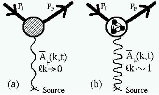
Figure 1: Substructure is not seen by the long wave-length modes (a). Due to functional dependence on matrix coordinates, the short wave-length modes can probe inside the bound state (b). $\ell$ and $\bar{A}_{\mu}(k,t)$ represent the size of the bound state and the Fourier modes, respectively.

In the limit $\ell|k|\rightarrow 0$ (long wave-length regime), the field $A_{\mu}$ is not involved by $X$ matrices mainly. It means that the fields appear to be nearly constant inside the bound state, and in rough estimation we have

$${\rm e}^{ik_{i}X^{i}}\sim{\rm e}^{ik_{i}X^{i}_{\rm c.m.}}.$$ (3.4)

So in this limit we expect that the substructure and consequently non-commutativity will not be seen; Figure-1a. As the consequence, after interaction with a long wave-length mode, it is not expected that the bound state jump to another energy level different from the first one. It should be noted that the c.m. dynamics can be affected as well in this case.

In the limit $\ell|k|=$finite (short wave-length regime), the fields depend on coordinates $X$ inside the bound state, and so the substructure responsible for non-commutativity should be probed; Figure-1b. In fact, we know that the non-commutativity of D0-brane coordinates is the consequence of the strings which are stretched between D0-branes. So, by these kinds of scattering processes, one should be able to probe both D0-branes (as point-like objects), and the strings stretched between them. In this case, it is completely expectable that the energy level of the incoming and outgoing bound states will be different, since the ingredients of bound state substructure can absorb quanta of energy from the incident wave. In this case the c.m. dynamics can be affected in a novel way by the interaction of the substructure with the external fields (the Van der Waals effect).

In general case, one can gain more information about the substructure of a bound state by analysing the ‘recoil’ effect on the source. To do this, one should be able to include the dynamics of the source in the formulation. Considering the dynamics of source, in the terms of quantized field theory, means that we consider the processes in which the source and the target exchange ‘one quanta of gauge field’ with definite wave-length and frequency, though off-shell, as $A_{\mu}(x,t)\sim\epsilon_{\mu}{\rm e}^{ik_{i}x^{i}-i\omega t}$. This kind of process is shown in Figure-2.

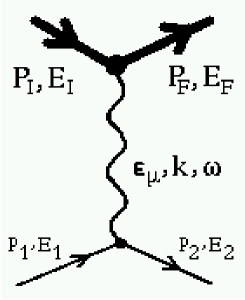
Figure 2: Exchange of one photon between a D0-brane bound state (thick lines) and another source (thin lines).

3.2 Path Integral Quantization

In this subsection we consider the quantisation of D0-brane dynamics, using the path integral method. The theory on the world-line enjoys a gauge symmetry, defined by the transformations (2.3). We should fix this symmetry, and here we use simply the temporal gauge, defined by the condition $a_{t}(t)\equiv 0$. So after the Wick rotation $t\rightarrow-it$ and $A_{0}\rightarrow-iA_{0}$, we have the following expression for the path integral of our system:

$$\langle X_{F},t_{F}|X_{I},t_{I}\rangle\sim\int[DX][Da_{t}]\;\delta(a_{t})\;\det|\frac{\delta a_{t}}{\delta\Lambda}|\;{\rm e}^{-S_{{\rm D0}}[X,a_{t}]},$$ (3.5)

in which $\delta(a_{t})$ supports the gauge fixing condition, and $\det|\frac{\delta a_{t}}{\delta\Lambda}|$ is the determinant which arises by variation of gauge fixing condition, and finally $S_{{\rm D0}}[X,a_{t}]$ is the action (2.7) evaluated between $(X_{F},t_{F})$ and $(X_{I},t_{I})$, as ‘Final’ and ‘Initial’ conditions. The variation of gauge fixing condition can be calculated in our case easily, and it is found to be (for $U(X,t)=\exp(-i\Lambda)$):

$$a_{t}=0\rightarrow a^{\prime}_{t}=\delta a_{t}=-iU^{\dagger}\partial_{t}U=-\partial_{t}\Lambda(X,t)+O(\Lambda^{2}),$$ (3.6)

and consequently we have $\frac{\delta a_{t}(t)}{\delta\Lambda(t^{\prime})}=-\partial_{t}\delta(t-t^{\prime})$. So, we see that the determinant and consequently the corresponding ghosts are decoupled from our dynamical fields $X$’s . So, up to a normalization factor, we have for the above expression of path integral:

$$\langle X_{F},t_{F}|X_{I},t_{I}\rangle\sim\int[DX]\;{\rm e}^{-S_{{\rm D0}}[X,a_{t}\equiv 0]}.$$ (3.7)

To calculate the path integral in a general background we have to use the perturbation expansion in the powers of charge $q$; this expansion is also valid for the weak external fields $(A_{0},A_{i})$. So we have

$$\langle X_{F},t_{F}|X_{I},t_{I}\rangle \sim \int[DX]\;{\rm e}^{-\int_{t_{I}}^{t_{F}}dt\;{\rm Tr\;}({\frac{1}{2}}m\dot{X}_{i}\dot{X}^{i}+m\frac{[X^{i},X^{j}]^{2}}{4(2\pi l^{2})^{2}})}$$ (3.8)

$$\times\sum_{n=0}^{\infty}\frac{q^{n}}{n!}\;\bigg{\{}i\int_{t_{I}}^{t_{F}}dt\;{\rm Tr\;}\bigg{(}\dot{X}^{i}A_{i}(X,t)+A_{0}(X,t)\bigg{)}\bigg{\}}^{n}.$$

As mentioned before, from the point of view of D0-brane dynamics, the commutator potential $[X^{i},X^{j}]^{2}$ is responsible for the formation of D0-brane bound states [27]. Though the problem of finding the full set of eigen-energies and eigen-vectors of the corresponding Hamiltonian is a very hard task, we assume that this full set is at hand. It is logical to separate the c.m. variables from the internal ones; we show those of c.m. by momenta $P_{\rm c.m.}$ and $|P_{\rm c.m.}\rangle$, and those of internal ones by energy $E_{\{n\}}$ and $|\{n\}\rangle$, in which $\{n\}$ presents all of the quantum numbers associated to the internal dynamics. We recall that the c.m. is free in the case of $q=0$. It is worth to recall that, in general we expect that the eigen-energies have the general form of $E_{\{n\}}=g(\{n\})\ell^{-1}$, with $g(\{n\})$ as a function of quantum numbers $\{n\}$, and as well the condition

$$\langle X|\{n\}\rangle\rightarrow 0,\;\;\;\;\;\;{\rm for}\;\;|X|\gg\ell,$$ (3.9)

for the wave-functions, with $\ell\sim m^{-1/3}l^{2/3}$ the size scale of the bound state we mentioned in before. As any other quantum mechanical system, for the case $q=0$ the general expression of the propagator can be used:

$$\langle X_{2},t_{2}|X_{1},t_{1}\rangle_{q=0}=\sum_{P_{\rm c.m.}}\sum_{\{n\}}\langle X_{2}|P_{\rm c.m.},\{n\}\rangle\langle P_{\rm c.m.},\{n\}|X_{1}\rangle{\rm e}^{-(\frac{P_{\rm c.m.}^{2}}{2Nm}+E_{\{n\}})(t_{2}-t_{1})},$$ (3.10)

with definition $|P_{\rm c.m.},\{n\}\rangle\equiv|P_{\rm c.m.}\rangle\otimes|\{n\}\rangle$. We now can insert the propagator above in last expression (3.8), with this care that the perturbation expansion have terms involved by velocity $\dot{X}$. Based on the standard representation of ‘slicing’ we use for the path integrals, finally the following expression for the first order of perturbation will be found (see [30]):

$$\langle X_{F},t_{F}|X_{I},t_{I}\rangle \sim \langle X_{F},t_{F}|X_{I},t_{I}\rangle_{q=0}$$ (3.11)

$$+ i{\cal N}\lim_{\Delta t\rightarrow 0}\sum_{k=1}^{n}\int d^{d}X_{k-1}d^{d}X_{k}d^{d}X_{k+1}\times\langle X_{F},t_{F}|X_{k+1},t_{k+1}\rangle_{q=0}\times$$

$$2\Delta t\cdot{\rm Tr\;}\bigg{(}q\frac{X^{i}_{k+1}-X^{i}_{k-1}}{2\Delta t}A_{i}(X_{k},t)+qA_{0}(X_{k},t)\bigg{)}\times$$

$$\langle X_{k-1},t_{k-1}|X_{I},t_{I}\rangle_{q=0}\times{\rm e}^{-S_{q=0}[k,k-1;\Delta t]}\;\;{\rm e}^{-S_{q=0}[k+1,k;\Delta t]}$$

$$+ O(q^{2}),$$

in which $t_{j}-t_{I}=j\cdot\Delta t$ and $t_{F}-t_{I}=(n+1)\Delta t$. In above $S_{q=0}[j,j+1;\Delta t]$ is the value of the action in the exponential of (3.8) evaluated between the points $(X_{j},t_{j})$ and $(X_{j+1},t_{j+1})$ ($1\leq j\leq n$) by limit $\Delta t\rightarrow 0$. The normalization constant ${\cal{N}}$ contains sufficient powers of $\Delta t$ to make the final result finite and independent of $\Delta t$. The sum $\sum_{k}$ is coming from slicing the potential term $\int dt{\rm Tr\;}(\dot{X}\cdot A+A_{0})$ in path integral (3.8), and it eventually will change to the time integral $\int dt$ over the intermediate ‘times’ in which the interaction occur. It is worth to recall that the spatial integrals like $\int d^{d}X$ are in fact as $\int\prod_{a=0}^{N^{2}-1}d^{d}X_{a}$. We mention that for the velocity independent term $A_{0}(X,t)$, the integrals of $d^{d}X_{k\pm 1}$ can be done to get the new propagators, and after the change $X_{k}\rightarrow X$, we simply find the expression like

$$\sim i\int_{t_{I}}^{t_{F}}dt\int d^{d}X\;\langle X_{F},t_{F}|X,t\rangle_{q=0}{\rm Tr\;}\bigg{(}qA_{0}(X,t)\bigg{)}\langle X,t|X_{I},t_{I}\rangle_{q=0}+O(q^{2}),$$ (3.12)

which is the familiar expression for the velocity independent interactions.

For many practical aims, we should find the S-matrix elements between states with definite momenta and energies; Figure-3. This can be done by the proper transformations on the amplitudes $\langle X_{F},t_{F}|X_{I},t_{I}\rangle$ in the coordinate space.

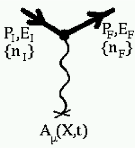
Figure 3: The graph for the transition amplitude between states with definite c.m. momenta and energies $(P,E)$, and internal energy specified by the quantum numbers $\{n\}$.

Due to less knowledge about the propagator (3.10), the last expression (3.11) still can not be used for the actual calculations. As mentioned in before, we expect that the spatial integrations $\int d^{d}X$ find their main contribution from the volume of bound state $V\sim\ell^{d}$. So as an approximation and to know a little more about the result, we may ignore the commutator potential, but doing integrations in the finite volume $V\sim\ell^{d}$, or in the case, we simply put $\int d^{d}X_{a}\sim\ell^{d}$, for $a\neq 0=$c.m. By doing this, we can verify the general aspects about the probing of the substructure of the bound state, discussed in the previous subsection.

3.3 Effective Interaction Vertex Of Photon And ‘Free’
D0-Branes

In the considerations of the previous subsection, the background $(A_{0}(x,t),A_{i}(x,t))$ was taken to be arbitrary. Here we take the example in which the D0-branes interact with a monotonic incident wave, defined by the condition $\bar{A}_{\mu}(k^{\prime},\omega^{\prime})=\epsilon_{\mu}\delta^{d}(k^{\prime}-k)\delta(\omega^{\prime}-\omega)$, with $\epsilon_{\mu}$ as the polarization vector, and the following definition for the Fourier modes:

$$\bar{A}_{\mu}(k^{\prime},\omega^{\prime})\equiv\frac{1}{(2\pi)^{d+1}}\int d^{d}x\;dt\;A_{\mu}(x,t)\;{\rm e}^{-ik_{i}^{\prime}x^{i}+i\omega^{\prime}t}.$$ (3.13)

So the corresponding gauge field is $A_{\mu}(X,t)\sim\epsilon_{\mu}\exp(ik_{i}X^{i}-i\omega t)$. Besides, here we ignore the commutator potential, and consequently it is assumed that all of the $N^{2}$ degrees of freedom, including those $N$ ones which describe the position of D0-branes, are free for $q=0$. So we have the following expression for the path integral:

$$\langle X_{F},t_{F}|X_{I},t_{I}\rangle \sim \int[DX]\;{\rm e}^{-\int_{t_{I}}^{t_{F}}dt\;{\rm Tr\;}({\frac{1}{2}}m\dot{X}_{i}\dot{X}^{i})}$$ (3.14)

$$\times\bigg{\{}1+iq\int_{t_{I}}^{t_{F}}dt\;{\rm Tr\;}\bigg{(}\dot{X}^{i}A_{i}(X,t)+A_{0}(X,t)\bigg{)}+O(q^{2})\bigg{\}}.$$

A similar theory for a charged particle in ordinary space is considered in the Appendix-A, to extract the field theory vertex function of the coupling of a ‘photon’ to incoming–outgoing charged particles. So the result of the path integral above, can be considered as the ‘matrix coordinate’ version of the example of the Appendix-A. We continue with an expression like that of (3.11), as:

$$\langle X_{F},t_{F}|X_{I},t_{I}\rangle \sim \langle X_{F},t_{F}|X_{I},t_{I}\rangle_{\rm f.p.}$$ (3.15)

$$+ i{\cal N}\lim_{\Delta t\rightarrow 0}\sum_{k=1}^{n}\int d^{d}X_{k-1}d^{d}X_{k}d^{d}X_{k+1}\times\langle X_{F},t_{F}|X_{k+1},t_{k+1}\rangle_{\rm f.p.}\times$$

$$2\Delta t\cdot{\rm Tr\;}\bigg{(}q\frac{X^{i}_{k+1}-X^{i}_{k-1}}{2\Delta t}A_{i}(X_{k},t)+qA_{0}(X_{k},t)\bigg{)}\times$$

$$\langle X_{k-1},t_{k-1}|X_{I},t_{I}\rangle_{\rm f.p.}\times{\rm e}^{-S_{\rm f.p.}[k,k-1;\Delta t]}\;\;{\rm e}^{-S_{\rm f.p.}[k+1,k;\Delta t]}$$

$$+ O(q^{2}),$$

in which $S_{\rm f.p.}$ and $\langle\cdots\rangle_{\rm f.p.}$ are the action and the propagator of free particles, respectively; see Appendix-B for the explicit expressions. The integrations $d^{d}X_{k\pm 1}$ can be done to get new propagators, and after the change $X_{k}\rightarrow X$, we find:

$$\langle X_{F},t_{F}|X_{I},t_{I}\rangle \sim \langle X_{F},t_{F}|X_{I},t_{I}\rangle_{\rm f.p.}$$ (3.16)

$$+ i{\cal N}^{\prime}\int_{t_{I}}^{t_{F}}dt\int d^{d}X\;\;\langle X_{F},t_{F}|X,t\rangle_{\rm f.p.}\times$$

$${\rm Tr\;}\bigg{\{}q\bigg{(}\frac{X^{i}_{F}-X^{i}}{t_{F}-t}+\frac{X^{i}-X^{i}_{I}}{t-t_{I}}\bigg{)}A_{i}(X,t)+qA_{0}(X,t)\bigg{\}}\times$$

$$\langle X,t|X_{I},t_{I}\rangle_{\rm f.p.}+O(q^{2}).$$

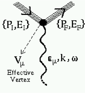
Figure 4: The graph for the transition amplitude between states with definite momenta and energies, specified with the set $\{P,E\}$, for all of $N^{2}$ degrees of freedom. Here we use some thin lines as incoming and outgoing states, to emphasize that these states are free before and after the vertex of interaction.

Up to now the gauge field can be in any arbitrary form. Also, since in this case we have ignored the commutator potential and so the degrees of freedom are free for $q=0$, we can easily use the momentum basis for the incoming-outgoing states; see Figure-4. So for the S-matrix element in momentum-energy basis, we have the expression:

$$S_{FI} \sim \prod_{a=0}^{N^{2}-1}\delta^{d}(P_{Fa}-P_{Ia})\delta(E_{Fa}-E_{Ia})$$ (3.17)

$$+ (\cdots)\int_{t_{I}}^{t_{F}}dt\int d^{d}X\int d^{d}X_{I}\;d^{d}X_{F}\prod_{a=0}^{N^{2}-1}\bigg{(}{\rm e}^{i(E_{Fa}t_{F}-E_{Ia}t_{I})}{\rm e}^{-i(P_{Fa}\cdot X_{Fa}-P_{Ia}\cdot X_{Ia})}\bigg{)}$$

$$\langle X_{F},t_{F}|X,t\rangle_{\rm f.p.}$$

$${\rm Tr\;}\bigg{(}iq\epsilon\cdot\bigg{(}\frac{X_{F}-X}{t_{F}-t}+\frac{X-X_{I}}{t-t_{I}}\bigg{)}{\rm e}^{ik\cdot X-i\omega t}+iq\epsilon_{0}{\rm e}^{ik\cdot X-i\omega t}\bigg{)}$$

$$\langle X,t|X_{I},t_{I}\rangle_{\rm f.p.}+O(q^{2}),$$

in which $E_{a}=P_{a}^{2}/(2Nm)$ for both $I$ and $F$ states (by convention ${\rm Tr\;}(T^{a}T^{b})=N\delta^{ab}$), and the symbol $A\cdot B$ is for the inner product $A_{i}B^{i}$. We recall that the subscripts $a$ and $b$ are counting the $N^{2}$ independent degrees of freedom associated with $N\times N$ hermitian matrices $X$ or $P$. Some of the integrations above can be done (see Appendix-B), and the resulting expression will be found to be:

$$S_{FI} \sim \prod_{a=0}^{N^{2}-1}\delta^{d}(P_{Fa}-P_{Ia})\delta(E_{Fa}-E_{Ia})$$ (3.18)

$$+ (\cdots)\delta^{d}(P_{F{\rm c.m.}}-P_{I{\rm c.m.}}-k)\delta\bigg{(}\sum_{a=0}^{N^{2}-1}(E_{Fa}-E_{Ia})-\omega\bigg{)}$$

$$\times \int\prod_{b=1}^{N^{2}-1}d^{d}\hat{X}_{b}\;{\rm e}^{i(P_{Ib}-P_{Fb})\cdot\hat{X}_{b}}{\rm Tr\;}\bigg{(}iq\bigg{(}\epsilon\cdot(P_{F}+P_{I})+\epsilon_{0}\bigg{)}{\rm e}^{ik\cdot\hat{X}}\bigg{)}+O(q^{2}),$$

in which the second series of $\delta$-functions have appeared as supports of the total momentum and total energy conservations. The last expression contains ${\rm Tr\;}$and integrals over the matrix coordinates $\hat{X}$ (${\rm Tr\;}(\hat{X})=0$), and though the improved forms in some special cases ($N$=2 or in large-$N$ limit) are accessible, the result in general case is not known. We mention that such integrals for ordinary coordinates, as that of Appendix-A, can be calculated exactly. We can present the general form of the result as:

$$S_{FI} \sim \prod_{a=0}^{N^{2}-1}\delta^{d}(P_{Fa}-P_{Ia})\delta(E_{Fa}-E_{Ia})$$ (3.19)

$$+ (\cdots)\delta^{d}(P_{F{\rm c.m.}}-P_{I{\rm c.m.}}-k)\delta\bigg{(}\sum_{a=0}^{N^{2}-1}(E_{Fa}-E_{Ia})-\omega\bigg{)}$$

$$\bigg{(}iq\epsilon\cdot V(P_{Ia,Fa},k)+iq\epsilon_{0}V_{0}(P_{Ia,Fa},k)\bigg{)}+O(q^{2}).$$

in which $V^{\mu}(P_{Ia,Fa},k)$, as the effective vertex function (see Figure-4), has the general form:

$$V^{i}={\rm Tr\;}\bigg{(}(P^{i}_{F}+P^{i}_{I})H(P_{Ia,Fa},k)\bigg{)}$$ (3.20)

$$V^{0}={\rm Tr\;}\bigg{(}H(P_{Ia,Fa},k)\bigg{)},$$

with $H(P_{Ia,Fa},k)$ as a matrix, depending on $P_{Ia}$, $P_{Fa}$ ($a=1,\cdots,N^{2}-1$, $a\neq{\rm c.m.}$) and $k$. In the case of ordinary coordinates for covariant theory we find simply $V^{\mu}\sim(p_{I}+p_{F})^{\mu}$; see Appendix-A.

4 Which Field Theory?

By the studies like those of [31], it is understood that the world-line theory of a charged particle in ordinary space, in presence of the gauge field background $A_{\mu}(x)$ can be corresponded to the second quantized field theory of interaction of charges and photons, something similar to the theory we imagine for the case of interaction of electrons and photons. The corresponding action may be presented as (with $\dot{x}=dx/d\tau$)

$$S=\int d\tau\;({\frac{1}{2}}m\dot{x}^{2}-q\dot{x}^{\mu}A_{\mu}(x)).$$ (4.1)

As an example, in the Appendix-A we derived the field theory vertex function for the interaction of a photon with the currents of incoming–outgoing charged particles. In the previous section we developed the basic elements of the world-line formulation of the interaction of D0-brane bound states with 1-form RR photons. Particularly, we showed how various amplitudes can be calculated in principle by the world-line theory, at least in the perturbative regime. In this section we want to discuss ‘which field theory’ can be corresponded to the amplitudes, calculated by the world-line theory. This is like the same relation that we consider in String Theory, between field theories in space-time and theories which are living on the world-sheet of strings. As we saw in previous section, our knowledge about the exact values of the amplitudes is restricted, and hence the discussion here will be based on some qualitative considerations. It remains for future studies to check the relation quantitavely, in particular by comparing the amplitudes as observable quantities.

Probably one of the most guiding observations is the ‘matrix’ nature of the gauge fields in the world-line formulation. Due to functional dependence of the gauge fields on matrix coordinates, the gauge fields $A^{\mu}(X)$ in our theory are $N\times N$ hermitian matrices, and so the gauge fields have the usual expansion in the matrix basis:

$$A^{\mu}(X)=A^{\mu}_{a}(X_{b})T^{a},\;\;\;\;\;\;\;A^{\mu}_{a}(X_{b})\equiv\frac{1}{N}{\rm Tr\;}(A^{\mu}(X)T^{a}),$$ (4.2)

in which $A^{\mu}_{a}(X_{b})$ are some functions (numbers) depending on the components of the matrix coordinates. The most famous ‘matrix’ gauge fields we know are those of non-Abelian gauge theories. Now, it is tempting to see what kind of relation between these two kinds of matrix gauge fields can be verified.

The best base we found for the possible relation mentioned in above is the suggested relation of [4], as the map between field configurations of non-commutative and ordinary gauge theories. The suggested map preserves the gauge equivalence relation, and it is emphasised that, due to different natures of the gauge groups, this map can not be an isomorphism between the gauge groups. Now in our case, it will be interesting to study the properties of the map between non-Abelian gauge theory and gauge theory associated with matrix coordinates; on one side the quantum theory of matrix fields, and on the other side the quantum mechanics of matrix coordinates. It will be helpful to do some imaginations in this direction. Since for the consideration we have in below there is no essential difference between fermions and bosons, we take the example of the interaction of a fermionic matter field with the external non-Abelian gauge field ${\cal A}_{\mu}(x)$, which is described by the action

$$S=\int d^{d+1}x\;\bigg{(}\bar{\psi}(i\gamma^{\mu}\partial_{\mu}-m)\psi-g{\rm Tr\;}(J^{\mu}{\cal A}_{\mu})\bigg{)},$$

$${\cal A}^{\mu}(x)={\cal A}^{\mu}_{a}(x)T^{a},$$

in which the term $J^{\mu}{\cal A}_{\mu}$ is responsible for the interaction; it may be chosen as that of the minimal coupling $J_{\mu}^{a}=i\bar{\psi}\gamma_{\mu}T^{a}\psi$. Gauge invariance specifies the behaviour of the current $J_{\mu}$ under the gauge transformations to be $J(x)\rightarrow J^{\prime}(x)=U^{\dagger}J(x)U$. Though here we are treating the gauge field as a fixed background, in general we can add the kinetic term of gauge fields by the action:

$$S_{{\rm gauge}}=\int d^{d+1}x\;{\rm Tr\;}(\frac{-1}{4}{\cal F}^{\mu\nu}{\cal F}_{\mu\nu}),$$

$${\cal F}^{\mu\nu}(x)={\cal F}^{\mu\nu}_{a}(x)T^{a},\;\;{\cal F}_{\mu\nu}=[{\cal D}_{\mu},{\cal D}_{\nu}],$$

with definition ${\cal D}_{\mu}\equiv\partial_{\mu}-ig{\cal A}_{\mu}$. On the world-line theory side, we have the theory of matrix coordinates. Let us, for the moment, forget that the world-line theory considered so far is in the non-relativistic limit, and consider things in a covariant theory. So, one may have something like the action below in the world-line theory:

$$S[X]=\int d\tau\;{\rm Tr\;}\bigg{(}{\frac{1}{2}}mD_{\tau}X_{\mu}D_{\tau}X^{\mu}-qD_{\tau}X^{\mu}A_{\mu}(X)+\cdots\bigg{)},$$ (4.5)

in which to make things easier, we have dropped any kind of potentials, including the commutator potential of D0-branes. In above, $\tau$ is parametrizing the world-line, $D_{\tau}=\partial_{\tau}+i[a_{\tau},\;]$ is the covariant derivative along the world-line, and $a_{\tau}$ is the world-line gauge field . The gauge field $A(X)$ depends on the symmetrized products of $X$’s. In the same spirit of the transformations in the world-line theory of D0-branes, we can take

$$X^{\mu} \rightarrow \tilde{X}^{\mu}=U^{\dagger}X^{\mu}U,$$

$$a_{\tau} \rightarrow \tilde{a}_{\tau}=U^{\dagger}a_{\tau}U-iU^{\dagger}\partial_{\tau}U,$$

$$A_{\mu}(X) \rightarrow \tilde{A}_{\mu}(\tilde{X})=U^{\dagger}A_{\mu}(X)U-iU^{\dagger}\delta_{\mu}U,$$ (4.6)

as the gauge transformation in the covariant theory, with $U=\exp(-i\Lambda(X,\tau))$. We mention that, $D_{\tau}X^{\mu}$ transforms as follows under the transformation: $D_{\tau}X^{\mu}\rightarrow\tilde{D}_{\tau}\tilde{X}^{\mu}=U^{\dagger}D_{\tau}X^{\mu}U$. Following relations (2.14) and (2.15), we can define the field strength as follows:

$$F_{\mu\nu}(X)\equiv\delta_{\mu}A_{\nu}(X)-\delta_{\nu}A_{\mu}(X),$$ (4.7)

and so the field strength transforms as: $F_{\mu\nu}\rightarrow\tilde{F}_{\mu\nu}=U^{\dagger}F_{\mu\nu}U$; see equation (2.3). Now, we want to sketch the map between the field theory in space-time and the world-line theory of a charged particle in a matrix space. It is natural to assume that the map should relate the objects in two theories as is shown in the Table-1.

Non-Abelian Field Theory	$\Leftrightarrow$	Gauge Theory On Matrix Space
${\cal A}^{\mu}(x)={\cal A}^{\mu}_{a}(x)T^{a}$	$\sim$	$A^{\mu}(X)+$ gauge trans. terms
${\cal F}^{\mu\nu}(x)={\cal F}^{\mu\nu}_{a}(x)T^{a}$	$\sim$	$F^{\mu\nu}(X)$
$J^{\mu}(x)=J^{\mu}_{a}(x)T^{a}$	$\sim$	$D_{\tau}X^{\mu}$
$\Lambda(x)=\Lambda_{a}(x)T^{a}$	$\sim$	$\Lambda(X)$

Table 1: The quantities which should be related by the map in two theories. $\Lambda$ is the symbol for the gauge transformation parameter in two theories.

We mention, 1) it is enough that the gauge fields are related up to a gauge transformation, 2) the objects in both sides are matrices, and 3) the field strengths and currents of the two theories transform identically under the gauge transformations.

Since in this case, we have matrices of equal sizes in both sides, it may be considered as a case in which one is able to find a one-to-one map between two theories. In particular, the one-to-one correspondence between the currents of two theories, i.e., $J^{\mu}$ and $D_{\tau}X^{\mu}$, suggests to verify whether such a one-to-one map can be defined or not. The case for the gauge fields ${\cal A}_{\mu}(x)$ and $A_{\mu}(X)$ appears to be a little more subtle, because, though the gauge fields in both sides are matrices, but the numbers of the independent functions of gauge fields do not match. In the side of ordinary gauge fields ${\cal A}_{\mu}(x)$, we have $N^{2}\cdot(d+1)$ independent functions. In the matrix coordinates side, we know how to construct functionals on matrix space: once a function on ordinary space as $f(x)$ is introduced, we can find its matrix coordinates version $f(X)$ by the non-Abelian Taylor or Fourier expansions, relations (2.5) and (3.1). So in the matrix coordinates side, the gauge field $A_{\mu}(X)$ is constructed just by $1\cdot(d+1)$ functions. In other words, in the matrix theory side, since the gauge fields $A_{\mu}(X)$ are matrices due to their functional dependence on matrix coordinates $X$, all of the components of the gauge field, defined in (4.2), are non-zero and specified in each direction by one function. One nice example is the plane wave of Subsec.3.3. The counting above will be modified by considering the gauge symmetry, but the mismatch will not be removed. So by this way of counting, finding a one-to-one map seems to be out of hand. It remains for future studies, to see whether such a mismatch between the number of the functions can find an explanation, to provide the definition of a one-to-one map .

In [13] a conceptual relation between the above map and the ideas concerned in special relativity is mentioned; see also [23, 24, 25]. According to an interpretation of the special relativity program, it can be meaningful if the ‘coordinates’ and the ‘fields’ in our physical theories have some kinds of similar characters. As an example, we observe that both the space-time coordinates $x^{\mu}$ and the electromagnetic potentials $A^{\mu}(x)$ transform equivalently (i.e., as a $(d+1)$-vector) under the boost transformations. Also, by this way of interpretation, the super-space formulations of supersymmetric field and superstring theories are the natural continuation of the special relativity program. In the case of above mentioned map, it may be argued that the relation between ‘matrix coordinates’ and ‘matrix fields’ (gauge fields of a non-Abelian gauge theory) is one of the expectations which is supported by the spirit of the special relativity program. We recall that the symmetry transformations of gauge theory on matrix space appeared to be similar to those of non-Abelian gauge theories, relations (2.3) and (2.3).

Finally, we should recall that, the theory which was considered in previous sections, was a non-relativistic theory. As noted before, to approach a covariant theory, the natural assumption is to interpret things as the light-cone gauge formulation of a covariant theory. It is the same approach by M(atrix) model conjecture [6], and in particular its finite-$N$ version [11]. Also the map we discussed in above between the D0-brane theory and gauge theory, should be considered for the light-cone formulation of the gauge theory side [32]. In the light-cone gauge formulation the non-relativistic mass $m$ is interpreted as the unit of longitudinal momentum, as $p_{+}=m$. Also we mention that, to match the amplitudes by world-line formulation with amplitudes by the field theory, the normalizations of the wave functions are different between the non-relativistic and light-cone gauge interpretations.

5 Conclusion And Discussion

In this work we provide the basic elements of the interaction of D0-brane bound states and 1-form RR photons, by the world-line formulation. At the classical level, we checked that the action is invariant under the gauge transformation of the gauge fields in the bulk theory. Also, due to matrix nature of the coordinates, we see that a new symmetry transformations exist, which under these new ones the gauge fields transform as gauge fields of a non-Abelian gauge theory. We interpret this observation as the case in which “the fields rotate due to rotation of coordinates”. We derived the Lorentz-like equations of motion, and the covariance of the equations are checked under the symmetry transformations. It is seen that the c.m. is ‘white’ or ‘colourless’ with respect to the $SU(N)$ sector of the background fields.

At the quantum level, we developed the perturbation theory of the interaction of D0-branes with the RR gauge fields. In particular, using the path integral method, we write down the expression of the propagator in the first order of perturbation, which can be converted to the amplitudes of the scattering processes by an arbitrary external source. It is discussed that how the functional dependence of gauge fields provides the base for probing the substructure of the bound states.

We discussed the possibility that the theory on the world-line of D0-branes can be mapped, maybe by a one-to-one map, to the non-Abelian gauge field theory.

One natural extension of the studies in this work can be for the supersymmetric case. Particularly in the case of maximal supersymmetry ($d=9$), we have the D0-branes of M(atrix) model, coupled to the 1-form RR background. As mentioned in Introduction, in the M(atrix) model picture D0-branes are assumed to be the super-gravitons of the 11-dimensional super-gravity in the light-cone gauge, and in particular they play in the case the role of the ‘photons’ of the 1-form RR field in 10 dimensions. The interaction of one D0-brane with a bound state of D0-branes is studied in the context of M(atrix) model, and according to the M(atrix) model interpretation, the commutator potential is responsible for the interaction of the single D0-brane (maybe viewed as one RR photon) and the bound state. The known results are those of different orders of loop calculations. It will be interesting to check whether the perturbation expansion in charge $q$ of this work, can reproduce the loop expansion results of M(atrix) model.

Another extension of the studies of this work, can be for including the gravitational effects, specificaly by considering non-flat metrics. The comparison to the M(atrix) model calculations also can be done in this case.

Acknowledgement: The author is grateful to Theory Group of INFN Section in ‘Tor Vergata University’, specially to A. Sagnotti, for kind hospitality. The careful readings of manuscript by M. Hajirahimi, and specially S. Parvizi are acknowledged. The author uses the grant under the executive letter no. $\frac{3/3746}{79/9/7}$, by the Ministry of Science, Research and Technology of Iran.

Appendix A Perturbation Theory Of A Charged Particle In
Ordinary Space By Path Integral Method

As an exercise, and to complete the basics of present paper, here we review the perturbation theory of a charged particle in electromagnetic background. Particularly, we extract the vertex function of the coupling of a photon to incoming–outgoing (bosonic) charged particles. In contrast to the non-relativistic theory of the paper, here we consider the covariant example. A good reference for these discussions is [30]. The action we use, initially in Euclidean space-time, is simply

$$S=\int d\tau\;({\frac{1}{2}}m\dot{x}^{2}-iq\dot{x}^{\mu}A_{\mu}(x)),$$ (A.1)

We begin with the expression similar to the formula (3.11) of the text as:

$$\langle x_{F},\tau_{F}|x_{I},\tau_{I}\rangle \sim \langle x_{F},\tau_{F}|x_{I},\tau_{I}\rangle_{\rm f.p.}$$ (A.2)

$$+ i{\cal N}\lim_{\Delta\tau\rightarrow 0}\sum_{k=1}^{n}\int d^{d+1}x_{k-1}d^{d+1}x_{k}d^{d+1}x_{k+1}\times\langle x_{F},\tau_{F}|x_{k+1},\tau_{k+1}\rangle_{\rm f.p.}\times$$

$$2\Delta\tau\cdot\bigg{(}q\frac{x^{\mu}_{k+1}-x^{\mu}_{k-1}}{2\Delta\tau}A_{\mu}(x_{k},\tau)\bigg{)}\times\langle x_{k-1},\tau_{k-1}|x_{I},\tau_{I}\rangle_{\rm f.p.}\times$$

$${\rm e}^{-S_{\rm f.p.}[k,k-1;\Delta\tau]}\;\;{\rm e}^{-S_{\rm f.p.}[k+1,k;\Delta\tau]}+O(q^{2}),$$

in which the normalization constant ${\cal N}$ contains sufficient powers of $\Delta\tau$ to regulate the final result, and we have the following relations:

$$\langle x_{2},\tau_{2}|x_{1},\tau_{1}\rangle_{\rm f.p.}\sim{\rm e}^{\frac{-m(x_{2}-x_{1})^{2}}{2(\tau_{2}-\tau_{1})}}\sim\int d^{d+1}l\;\exp\bigg{(}il\cdot(x_{2}-x_{1})-i\frac{l^{2}}{2m}(\tau_{2}-\tau_{1})\bigg{)},$$ (A.3)

$$S_{\rm f.p.}[j+1,j;\Delta\tau]=\frac{m(x_{j+1}-x_{j})^{2}}{2\Delta\tau},$$ (A.4)

with $A\cdot B=A^{\mu}B_{\mu}$. Doing integrations $dx_{k\pm 1}$ to replace new propagators, and after the change $x_{k}\rightarrow x$, we will find:

$$\langle x_{F},\tau_{F}|x_{I},\tau_{I}\rangle \sim \langle x_{F},\tau_{F}|x_{I},\tau_{I}\rangle_{\rm f.p.}+i{\cal N}^{\prime}\int_{\tau_{I}}^{\tau_{F}}d\tau\int d^{d+1}x\;\langle x_{F},\tau_{F}|x,\tau\rangle_{\rm f.p.}\times$$ (A.5)

$$\bigg{\{}q\bigg{(}\frac{x_{F}-x}{\tau_{F}-\tau}+\frac{x-x_{I}}{\tau-\tau_{I}}\bigg{)}\cdot A(x)\bigg{\}}\times\langle x,\tau|x_{I},\tau_{I}\rangle_{\rm f.p.}+O(q^{2}),$$

From now on we restrict the calculation to the plane wave $A_{\mu}(x)\sim\epsilon_{\mu}{\rm e}^{ik_{\nu}x^{\nu}}$. To find the S-matrix elements, it is usual to go to the momentum space, and we have the expression

$$S_{FI} \sim \delta^{d}(p_{F}-p_{I})\delta(E_{F}-E_{I})+\frac{{\cal N}^{\prime\prime}{\rm e}^{-im^{2}(\tau_{F}-\tau_{I})/2}}{\tau_{F}-\tau_{I}}\int_{\tau_{I}}^{\tau_{F}}d\tau\int d^{d+1}x\int d^{d+1}x_{I}\int d^{d+1}x_{F}$$ (A.6)

$${\rm e}^{-ip_{F}\cdot x_{F}}{\rm e}^{ip_{I}\cdot x_{I}}\langle x_{F},\tau_{F}|x,\tau\rangle_{\rm f.p.}\bigg{\{}{\rm e}^{ik\cdot x}\exp\bigg{(}iq\epsilon\cdot\bigg{(}\frac{x_{F}-x}{\tau_{F}-\tau}+\frac{x-x_{I}}{\tau-\tau_{I}}\bigg{)}\bigg{)}\bigg{\}}_{{\rm linear\;in}\;\epsilon}$$

$$\langle x,\tau|x_{I},\tau_{I}\rangle_{\rm f.p.}+O(q^{2}),$$

in which $p_{F}^{2}=p_{I}^{2}=-m^{2}$, and to make easier the calculation we have exponentiated the $\epsilon_{\mu}$; so we should keep only the linear term in $\epsilon$ finally. By using the momentum representation of the propagator $\langle\cdots\rangle_{\rm f.p.}$ we find:

$$S_{FI} \sim \delta^{d}(p_{F}-p_{I})\delta(E_{F}-E_{I})$$ (A.7)

$$+ (\cdots)\delta^{d}(p_{F}-p_{I}-k)\delta(E_{F}-E_{I}-k_{0})(iq\epsilon_{\mu}(p_{F}+p_{I})^{\mu})+O(q^{2}),$$

in which we recognize the field theory result $\epsilon\cdot(p_{F}+p_{I})$ for the vertex function (page 548 of [29]).

Appendix B Calculation Of S-Matrix Element For Matrix
Coordinates In Momentum Basis

Here we present the derivation of (3.18), starting with (3.17). By using the definitions:

$$\langle X_{2},t_{2}|X_{1},t_{1}\rangle_{\rm f.p.}\sim\int\prod_{a=0}^{N^{2}-1}d^{d+1}L_{a}\;\exp\bigg{(}iL_{a}\cdot(X_{2a}-X_{1a})-i\frac{L_{a}^{2}}{2Nm}(t_{2}-t_{1})\bigg{)},$$ (B.1)

$$S_{\rm f.p.}[j+1,j;\Delta t]=\sum_{a=0}^{N^{2}-1}\frac{Nm(X_{j+1,a}-X_{j,a})^{2}}{2\Delta t},$$ (B.2)

we find for (3.17)

$$S_{FI} \sim \prod_{a=0}^{N^{2}-1}\delta^{d}(P_{Fa}-P_{Ia})\delta(E_{Fa}-E_{Ia})$$ (B.3)

$$+ (\cdots)\int_{t_{I}}^{t_{F}}dt\int d^{d}X\int d^{d}X_{I}\;d^{d}X_{F}\prod_{a=0}^{N^{2}-1}\bigg{(}{\rm e}^{i(E_{Fa}t_{F}-E_{Ia}t_{I})}{\rm e}^{-i(P_{Fa}\cdot X_{Fa}-P_{Ia}\cdot X_{Ia})}\bigg{)}$$

$$\int\prod_{b=0}^{N^{2}-1}d^{d+1}Q_{b}\;\exp\bigg{(}iQ_{b}\cdot(X_{Fb}-X_{b})-i\frac{Q_{b}^{2}}{2Nm}(t_{F}-t)\bigg{)}$$

$$\bigg{(}\sum_{c=0}^{N^{2}-1}\bigg{\{}\exp\bigg{(}iq\epsilon\cdot\bigg{(}\frac{X_{Fc}-X_{c}}{t_{F}-t}+\frac{X_{c}-X_{Ic}}{t-t_{I}}\bigg{)}\bigg{)}\bigg{\}}_{{\rm linear\;in}\;\epsilon}{\rm Tr\;}\bigg{(}T^{c}{\rm e}^{ik\cdot X-i\omega t}\bigg{)}$$

$$+{\rm Tr\;}\bigg{(}iq\epsilon_{0}{\rm e}^{ik\cdot X-i\omega t}\bigg{)}\bigg{)}$$

$$\int\prod_{e=0}^{N^{2}-1}d^{d+1}L_{e}\;\exp\bigg{(}iL_{e}\cdot(X_{e}-X_{Ie})-i\frac{L_{e}^{2}}{2Nm}(t-t_{I})\bigg{)}+O(q^{2}),$$

in which to make easier the calculation, we have exponentiated the $\vec{\epsilon}$; so we should keep only the linear term in $\epsilon$ finally. In above the symbol $A\cdot B$ is for the inner product $A_{i}B^{i}$. It is worth to recall that the spatial integrals like $\int d^{d}X$ are in fact as $\int\prod_{a=0}^{N^{2}-1}d^{d}X_{a}$. Here we leave the term $\epsilon_{0}$ for the reader. After doing the integrations on $d^{d}X_{I,F}$, we have:

$$S_{FI} \sim \prod_{a=0}^{N^{2}-1}\delta^{d}(P_{Fa}-P_{Ia})\delta(E_{Fa}-E_{Ia})+(\cdots)\int_{t_{I}}^{t_{F}}dt\int\prod_{a=0}^{N^{2}-1}d^{d}X_{a}{\rm e}^{i(E_{Fa}t_{F}-E_{Ia}t_{I})}$$ (B.4)

$$\int\prod_{b=0}^{N^{2}-1}d^{d+1}Q_{b}\;d^{d+1}L_{b}\;{\rm e}^{-i\frac{Q_{b}^{2}}{2Nm}(t_{F}-t)}{\rm e}^{-i\frac{L_{b}^{2}}{2Nm}(t-t_{I})}{\rm e}^{i(L_{b}-Q_{b})\cdot X_{b}}$$

$$\bigg{(}\sum_{c=0}^{N^{2}-1}\prod_{e=0}^{N^{2}-1}\delta^{d}\bigg{(}Q_{e}-P_{Fe}+\frac{q\epsilon\delta_{ce}}{t_{F}-t}\bigg{)}\delta^{d}\bigg{(}L_{e}-P_{Ie}+\frac{q\epsilon\delta_{ce}}{t-t_{I}}\bigg{)}$$

$$\bigg{\{}\exp\bigg{(}iq\epsilon\cdot X_{c}\bigg{(}\frac{-1}{t_{F}-t}+\frac{1}{t-t_{I}}\bigg{)}\bigg{)}\bigg{\}}_{{\rm linear\;in}\;\epsilon}{\rm Tr\;}\bigg{(}T^{c}{\rm e}^{ik\cdot X-i\omega t}\bigg{)}\bigg{)}$$

$$+O(q^{2}).$$

By using the $\delta$-functions we simply can do the integrations on $d^{d}Q$ and $d^{d}L$. Also, based on the fact that $\exp(ik\cdot X)=\exp(ik\cdot X_{\rm c.m.}{\bf 1}_{N})\exp(ik\cdot\hat{X})$, with ${\rm Tr\;}(\hat{X})=0$, we can do the integration on $d^{d}X_{0}=d^{d}X_{\rm c.m.}$. By recalling $E_{a}=P_{a}^{2}/(2Nm)$ for $I$ and $F$ states (convention ${\rm Tr\;}(T^{a}T^{b})=N\delta^{ab}$), and by the limits $t_{I}\rightarrow-\infty$ and $t_{F}\rightarrow\infty$, we arrive at:

$$S_{FI} \sim \prod_{a=0}^{N^{2}-1}\delta^{d}(P_{Fa}-P_{Ia})\delta(E_{Fa}-E_{Ia})$$ (B.5)

$$+ (\cdots)\delta^{d}(P_{F{\rm c.m.}}-P_{I{\rm c.m.}}-k)\delta\bigg{(}\sum_{a=0}^{N^{2}-1}(E_{Fa}-E_{Ia})-\omega\bigg{)}$$

$$\times \int\prod_{b=1}^{N^{2}-1}d^{d}\hat{X}_{b}\;{\rm e}^{i(P_{Ib}-P_{Fb})\cdot\hat{X}_{b}}\sum_{c=0}^{N^{2}-1}\bigg{\{}{\rm e}^{\frac{i}{m}q\epsilon\cdot(P_{Fc}+P_{Ic})}\bigg{\}}_{{\rm linear\;in}\;\epsilon}\!\!\!\;{\rm Tr\;}\bigg{(}T^{c}{\rm e}^{ik\cdot\hat{X}}\bigg{)}+O(q^{2}).$$

References

- [1] J. Polchinski, “Dirichlet-Branes And Ramond-Ramond Charges,” Phys. Rev. Lett. 75 (1995) 4724, hep-th/9510017.
- [2] E. Witten, “Bound States Of Strings And p-Branes,” Nucl. Phys. B460 (1996) 335, hep-th/9510135.
- [3] A. Connes, M.R. Douglas and A. Schwarz, “Noncommutative Geometry And Matrix Theory: Compactification On Tori,” JHEP 9802 (1998) 003, hep-th/9711162; M.R. Douglas and C. Hull, “D-Branes And The Noncommutative Torus,” JHEP 9802 (1998) 008, hep-th/9711165.
- [4] N. Seiberg and E. Witten, “String Theory And Noncommutative Geometry,” JHEP 9909 (1999) 032, hep-th/9908142.
- [5] H. Arfaei and M.M. Sheikh-Jabbari, “Mixed Boundary Conditions And Brane-String Bound States,” Nucl. Phys. B526 (1998) 278, hep-th/9709054; M.M. Sheikh-Jabbari, “More On Mixed Boundary Conditions And D-Branes Bound States,” Phys. Lett. B425 (1998) 48, hep-th/9712199.
- [6] T. Banks, W. Fischler, S.H. Shenker and L. Susskind, “M Theory As A Matrix Model: A Conjecture,” Phys. Rev. D55 (1997) 5112, hep-th/9610043.
- [7] T. Banks, “Matrix Theory,” Nucl. Phys. Proc. Suppl. 67 (1998) 180, hep-th/9710231; “TASI Lectures On Matrix Theory,” hep-th/9911068; D. Bigatti and L. Susskind, “Review Of Matrix Theory,” hep-th/9712072; W. Taylor, “ The M(atrix) Model Of M-theory,” hep-th/0002016; “M(atrix) Theory: Matrix Quantum Mechanics As A Fundamental Theory,” Rev. Mod. Phys. 73 (2001) 419, hep-th/0101126; R. Helling, “Scattering In Supersymmetric M(atrix) Models,” Fortschur. Phys. 48 (2000) 1229.
- [8] R.C. Myers, “Dielectric-Branes,” JHEP 9912 (1999) 022, hep-th/9910053.
- [9] W. Taylor and M. Van Raamsdonk, “Multiple Dp-Branes In Weak Background Fields,” Nucl. Phys. B573 (2000) 703, hep-th/9910052.
- [10] S. Parvizi and A.H. Fatollahi, “D-Particle Feynman Graphs And Their Amplitudes,” hep-th/9907146; A.H. Fatollahi, “Feynman Graphs From D-Particle Dynamics,” hep-th/9806201.
- [11] L. Susskind, “Another Conjecture About M(atrix) Theory,” hep-th/9704080.
- [12] A.H. Fatollahi, “On Non-Abelian Structure From Matrix Coordinates,” Phys. Lett. B512 (2001) 161, hep-th/0103262.
- [13] A.H. Fatollahi, “Electrodynamics On Matrix Space: Non-Abelian By Coordinates,” to appear in Eur. Phys. J. C, hep-th/0104210.
- [14] J. Polchinski, “TASI Lectures On D-Branes,” hep-th/9611050.
- [15] C.M. Hull, “Matrix Theory, U-Duality And Toroidal Compactifications Of M-Theory,” JHEP 10 (1998) 11, hep-th/9711179; H. Dorn, “Nonabelian Gauge Field Dynamics On Matrix D-Branes,” Nucl. Phys. B494 (1997) 105, hep-th/9612120.
- [16] M.R. Douglas, “D-Branes And Matrix Theory In Curved Space,” Nucl. Phys. Proc. Suppl. 68 (1998) 381, hep-th/9707228; “D-Branes In Curved Space,” Adv. Theor. Math. Phys. 1 (1998) 198, hep-th/9703056; M.R. Douglas, A. Kato and H. Ooguri, “D-Brane Actions On Kahler Manifolds,” Adv. Theor. Math. Phys. 1 (1998) 237, hep-th/9708012.
- [17] M.R. Garousi and R.C. Myers, “World-Volume Interactions On D-Branes,” Nucl. Phys. B542 (1999) 73, hep-th/9809100; “World-Volume Potentials On D-Branes,” JHEP 0011 (2000) 032, hep-th/0010122.
- [18] D. Kabat and W. Taylor, “Linearized Supergravity From Matrix Theory,” Phys. Lett. B426 (1998) 297, hep-th/9712185.
- [19] W. Taylor and M. Van Raamsdonk, “Angular Momentum And Long-Range Gravitational Interactions In Matrix Theory,” Nucl. Phys. B532 (1998) 227, hep-th/9712159; M. Van Raamsdonk, “Conservation Of Supergravity Currents From Matrix Theory,” Nucl. Phys. B542 (1999) 262, hep-th/9803003; W. Taylor and M. Van Raamsdonk, “Supergravity Currents And Linearized Interactions For Matrix Theory Configurations With Fermionic Backgrounds,” JHEP 9904 (1999) 013, hep-th/9812239.
- [20] A.A. Tseytlin, “On Non-Abelian Generalisation Of Born-Infeld Action In String Theory,” Nucl. Phys. B501 (1997) 41, hep-th/9701125.
- [21] W. Taylor and M. Van Raamsdonk, “D0-Branes In Weakly Curved Backgrounds,” Nucl. Phys. B558 (1999) 63, hep-th/9904095.
- [22] C. Ciocarlie, “On The Gauge Invariance Of The Chern-Simons Action For N D-Branes,” JHEP 0107 (2001) 028, hep-th/0105253.
- [23] A.H. Fatollahi, “D0-Branes As Confined Quarks,” talk given at “Isfahan String Workshop 2000, May 13-14, Iran,” hep-th/0005241.
- [24] A.H. Fatollahi, “D0-Branes As Light-Front Confined Quarks,” Eur. Phys. J. C19 (2001) 749, hep-th/0002021.
- [25] A.H. Fatollahi, “Do Quarks Obey D-Brane Dynamics?,” Europhys. Lett. 53(3) (2001) 317, hep-ph/9902414; “Do Quarks Obey D-Brane Dynamics?II,” hep-ph/9905484, to appear in Europhys. Lett.
- [26] A.H. Fatollahi, “Gauge Symmetry As Symmetry Of Matrix Coordinates,” Eur. Phys. J. C17 (2000) 535, hep-th/0007023.
- [27] U.H. Danielsson, G. Ferretti and B. Sundborg, “D-Particle Dynamics And Bound States,” Int. J. Mod. Phys. A11 (1996) 5463, hep-th/9603081; D. Kabat and P. Pouliot, “A Comment On Zero-Brane Quantum Mechanics,” Phys. Rev. Lett. 77 (1996) 1004, hep-th/9603127.
- [28] B. de Wit, “Supersymmetric Quantum Mechanics, Supermembranes And Dirichlet Particles,” Nucl. Phys. Proc. Suppl. B56 (1997) 76, hep-th/9701169; H. Nicolai and R. Helling, “Supermembranes And M(atrix) Theory,” hep-th/9809103; B. de Wit, “Supermembranes And Super Matrix Models,” hep-th/9902051.
- [29] G. Sterman, “An Introduction To Quantum Field Theory,” Cambridge University Press (1994).
- [30] L.H. Ryder, “Quantum Field Theory,” Cambridge University Press (1985).
- [31] M.J. Strassler, “Field Theory Without Feynman Diagrams: One-Loop Effective Actions,” Nucl. Phys. B385 (1992) 145, hep-ph/9205205.
- [32] R. Perry, “Hamiltonian Light-Front Field Theory And Quantum Chromodynamics,” hep-th/9407056; T. Heinzl, “Light-Cone Dynamics Of Particles And Fields,” hep-th/9812190; R. Venugopalan, “Introduction To Light Cone Field Theory And High Energy Scattering,” nucl-th/9808023; S.J. Brodsky, H-C Pauli and S. Pinsky, “Quantum Chromodynamics And Other Field Theories On The Light Cone,” Phys. Rept. 301 (1998) 299, hep-ph/9705477.