The $\nu=5/2$ quantum Hall state revisited: spontaneous breaking of the chiral fermion parity and phase transition between abelian and non-abelian statistics

Abstract

We review a recent development in the theoretical understanding of the $\nu=5/2$ quantum Hall plateau and propose a new conformal field theory, slightly different from the Moore–Read one, to describe another universality class relevant for this plateau. The ground state is still given by the Pfaffian and is completely polarized, however, the elementary quasiholes are charge $1/2$ anyons with abelian statistics $\theta=\pi/2$, which obey complete spin–charge separation. The physical hole is represented by two such quasiholes plus a free neutral Majorana fermion. We also compute the periods and amplitudes of the chiral persistent currents in both states and show that they have different temperature dependence. Finally, we find indications of a classical two-step phase transition between the new and the Moore–Read states, through a compressible state, which is characterized by the spontaneous breaking of a hidden ${\mathbb{Z}}_{2}$ symmetry corresponding to the conservation of the chiral fermion parity. We believe that this transition could explain the “kink” observed in the activation experiment for $\nu=5/2$.

1 Introduction

The nature of the first observed fractional quantum Hall (FQH) state, with even denominator of the filling factor $\nu=5/2$ [1, 2], remains obscure more than a decade. Its collapse with the increase of the tilted field [3] suggested that its ground state might be a spin-singlet, however, this turned out to be wrong. Shortly after the first challenge of this interpretation [4] a new experiment with the $\nu=5/2$ FQH state [5] confirmed that its ground state is indeed spin-polarized. The first spin-singlet state for the $\nu=5/2$ plateau, motivated by the wrong interpretation of the tilted field experiment, was introduced by Haldane and Rezayi [6] and besides other inconsistencies, such as the violation of the spin–statistics relation, non-unitarity and absence of modular invariance, turned out to be an excited state over the 331 ground state [7]; later it was found to describe a compressible state [8, 9] at the transition between weak and strong pairing phases of the p-wave BCS Hamiltonian, explaining why the so called Haldane–Rezayi state [6] is not a true FQH state.

The 1+1 dimensional conformal field theory (CFT), describing the FQH edge excitations in the thermodynamic limit, has proven to be a convenient tool for analyzing the universality classes of the FQH states [10, 7, 11]. The CFT approach became even more important after the recent experiment [12] showing that the chiral Luttinger liquid point of view is at best incomplete or at worst wrong. So far the most successful CFT for the $\nu=5/2$ FQH state has been proposed by Moore–Read (MR) [13, 9]. Numerical calculations [14] have shown that, after proper particle–hole (PH) symmetrization, the MR state seems to have a good overlap with the exact ground state for the $\nu=5/2$ plateau, and that this state most likely determines the universality class of the $\nu=5/2$ FQH state for zero temperature. However, since the PH symmetry is a characteristics of the universality class, it is rather strange that the MR Hamiltonian used in [14] is not PH symmetric. In this paper we try to interpret the results of [14] in a way to explain this peculiarity.

Another striking fact become apparent after the recent activation experiment [2]. The logarithmic plot of the longitudinal resistance $R_{xx}$, as a function of the inverse temperature, turned out to be non-linear. The slope suddenly changes around $T\sim 15$ mK [2], which was called “a kink” that these authors could not explain. We stress that the change of the slope of the diagonal resistance is a clear indication of a phase transition implying that there should be another incompressible phase at $\nu=5/2$, with a different energy gap, which like the MR state, is supposed to be completely polarized [5]. In other words, there should be another universality class, hence another (rational) CFT, which is relevant for the $\nu=5/2$ plateau. In this paper we propose a new universality class for the $\nu=5/2$ FQH plateau — a rational extension of the MR state — which we call the Extended Pfaffian (EPf) state. Although it may look innocent, this extension changes dramatically the structure of the excitations. In Sect. 3 we analyze the CFT for the EPf state and show that the minimal electric charge in this state is $1/2$ (in units in which the electron charge is $-1$) and the quasiparticle’s statistics is abelian. This has to be compared with the MR state where the minimal electric charge is $1/4$ and the statistics of quasiparticles is non-abelian [13, 15, 16, 17]. We recall that, the construction of the EPf state, together with the assumption that the energy gap in the FQH fluids has a universal component proportional to the quasihole’s electric charge, was able to explain [18] the non-monotonic structure [2] of the parafermionic Hall states in the second Landau level.

One more peculiarity of the MR state is the fact that its chiral fermion parity number is not conserved in the twisted sector, due to the non-abelian fusion rules of the quasiparticles, hence, the fermion parity is spontaneously broken in this sector. In Sect. 5 we show that this reduces the topological order of the MR state as compared to the double-layer 331 state [19, 7]. Recall that the MR state was interpreted [7, 8, 32] as a low-barrier (or high-tunneling) limit of the 331 state and the transition from 331 to the MR state could be characterized by the spontaneous breaking of this ${\mathbb{Z}}_{2}$ symmetry. Note that the fermion parity plays a fundamental role in finite geometries since the ground states of interacting fermionic systems are believed to be paramagnetic/diamagnetic for even/odd fermion parity [20, 21], in very much the same way like the free systems [22]; the latter is known as the Leggett conjecture [23].

Our analysis shows that the kink observed in the activation experiment at $\nu=5/2$ [2] is due to a classical two-step phase transition involving an intermediate compressible state. At low temperatures the system is in the MR phase, in which the chiral fermion parity ${\mathbb{Z}}_{2}$ symmetry is spontaneously broken. When the temperature becomes bigger than the activation energy for the MR state, the system undergoes a second order phase transition (in which the ${\mathbb{Z}}_{2}$ symmetry is restored) to a compressible state, which is topologically equivalent to the Composite Fermions (CF) Fermi liquid found before [4, 14, 24], and then a first order phase transition to the EPf state. Using the previous estimation of the energy gaps according to the gap ansatz in [18] we find in Sect. 4 that the gap of the EPf state is almost 3 times bigger than that of the MR state, i.e., $\Delta_{\mathrm{EPf}}=110$ mK and $\Delta_{\mathrm{MR}}=33$ mK for the sample of [2], which could explain the kink observed in the activation experiment [2], as well as the absence of fermion parity number in the MR state. It is also intriguing that similar kinks are seen also in the activation experiments for the neighboring FQH plateaux at $\nu=7/3$ and $8/3$, which suggests that this is probably a general phenomenon.

In Sect. 6 we discuss the PH symmetry of the MR and EPf states and reinterpret the numerical results of [14] in order to explain the absence of the PH symmetry in the MR state. In Sect. 7 we compute the contributions of all topologically inequivalent quasiparticles to the specific heat of the EPf state.

In Sect. 8 we describe how to derive the mesoscopic persistent currents of MR and EPf states directly from their effective CFTs, using the modular covariance of the CFT characters, in which the non-analytic factors of Cappelli–Zemba (CZ) [29] are included. We stress again that this approach is a complement and an alternative to the chiral Luttinger liquid description which is unsatisfactory [12]. We find that the persistent currents in the MR and EPf states are periodic functions of the magnetic flux with period exactly one flux quantum. The amplitudes of the persistent currents are the same at zero temperature, however, for finite temperatures the amplitude of the persistent current in the EPf state is always bigger than that in the MR state. This fact could be used in principle to detect any transition between the two states, e.g., in a SQUID experiment [25]. Both currents exhibit a universal non-Fermi liquid temperature behaviour and we find analytic formulae for the temperature dependence of the amplitudes in both limits of low and high temperatures.

In Sect. 9 we describe in more detail the above mentioned scenario for the phase transition between the MR and EPf states. Again we point out that this transition could possibly explain the kink observed in the activation experiment [2]. Some technical remarks are summarized in several appendices.

2 The Moore–Read state: the CFT coset point of view

Originally, the MR ground and excited states were introduced [13] as correlators of certain operators in a CFT based on the chiral algebra ${\widehat{u(1)}}\otimes\mathrm{Ising}$. For example, the ground state wave function (up to the standard Gaussian exponent) is expressed as a correlator of $2N$ “electron operators” [13, 19, 7]

$$\psi_{\mathrm{el}}(z)=\varphi(z):\mathrm{e}^{-i\sqrt{2}\phi(z)}:,$$ (1)

where $\varphi(z)$ is the neutral Majorana fermion in the Ising model and $:\mathrm{e}^{-i\sqrt{2}\phi(z)}:$ is the ${\widehat{u(1)}}$ vertex exponent representing the charged component of the electron [7], as follows

$$\Psi_{\mathrm{GS}}(z_{1},\ldots,z_{2N})=\langle\prod_{j=1}^{2N}\psi_{\mathrm{el}}(z_{j})\rangle=\mathrm{Pf}\left(\frac{1}{z_{i}-z_{j}}\right)\prod_{i<j}(z_{i}-z_{j})^{2}.$$ (2)

This polarized state was called paired in analogy with the real space BCS type wave function expressed by the Pfaffian [13, 7]. The stress energy tensor of the MR state is a sum of the ${\widehat{u(1)}}$ and the Ising contributions

$$T(z)=-\frac{1}{2}:\partial\phi(z)^{2}:-\frac{1}{2}:\varphi(z)\partial\varphi(z):$$ (3)

and has a central charge $c_{\mathrm{MR}}=3/2$. The elementary quasiholes are represented by

$$\psi^{\mathrm{MR}}_{\mathrm{q.h.}}(z)=\sigma(z):\mathrm{e}^{i\frac{1}{2\sqrt{2}}\phi(z)}:,\quad Q^{\mathrm{MR}}_{\mathrm{q.h.}}=1/4,\quad\Delta^{\mathrm{MR}}_{\mathrm{q.h.}}=1/8,$$ (4)

where $\sigma$ is the chiral spin–field of the Ising model with (neutral) CFT dimension $1/16$ and the normal ordered exponent represents the charged component of the quasihole. The quasiholes (4) have rather peculiar properties — their electric charge $Q^{\mathrm{MR}}_{\mathrm{q.h.}}$ differs from the denominator of the filling factor, they carry half-integer flux $\Phi^{\mathrm{MR}}_{\mathrm{q.h.}}=1/2$, so that must be created in pairs, their total CFT dimension is $\Delta^{\mathrm{MR}}_{\mathrm{q.h.}}=1/8$, however they obey non-abelian statistics [13, 26, 7, 11]. Note that for QH states with even-denominator $d_{H}$ the minimal electric charge is $Q_{\min}=1/(ld_{h})$, where $l$ is an even integer called the charge parameter — see Theorem 4.3 in [27]. A recent study of the MR state in the framework of the parafermionic FQH states [28, 16, 17], realized as coset constructions [11], has made the mechanism of clustering more transparent. In particular, the MR state is realized as an affine coset projection [11] $\widehat{su(2)}_{1}\oplus\widehat{su(2)}_{1}\to\left(\widehat{su(2)}_{1}\oplus\widehat{su(2)}_{1}\right)/\widehat{su(2)}_{2}$, in an abelian lattice theory of the type [11, 27] $(3|{}^{1}A_{1}{}^{1}A_{1})$, i.e., a theory with a $K$-matrix and a charge vector ${\underline{\mathrm{Q}}}$

$$K=\left[\matrix{3&1&1\cr 1&2&0\cr 1&0&2}\right],\quad{\underline{\mathrm{Q}}}=(1,0,0),$$

which is interpreted as removing the layer (or color) $su(2)$ symmetry. The above pair $(K,{\underline{\mathrm{Q}}})$ uniquely determines the Chern–Simons topological theory in the bulk and the coset projection is interpreted as gauging out the $\widehat{su(2)}_{2}$ layer symmetry, which produces a non-abelian topological effective theory for the bulk of the FQH fluid. The Chern–Simons effective field theory describing the bulk of the MR state has attracted much attention [16, 15] due to the peculiar properties of the non-abelian quasiparticles present there. We stress that the CFT on the $1+1$ dimensional boundary determines uniquely the topological field theory in the bulk [10]. Therefore, the pairing rule in the MR state (see Eq. (13) below), which gives rise to a ${\mathbb{Z}}_{2}$ orbifold CFT construction [19, 7], has crucial implications for the bulk effective field theory of the fermionic Pfaffian state.

The quasiholes wave functions, after the coset projection, can be obtained by symmetrization [11] of the wave functions of their parent counterparts and the non-abelian statistics is understood as a result of degeneration in the space of quasihole wave functions during this process. Another advantage of this projective construction is that the projected model inherits some structures, such as pairing rules and modular covariance, from its parent [11].

The chiral partition functions, $\chi_{l,\rho}(\tau,\zeta)={\mathop{\mathrm{tr}}\limits_{\quad{\mathcal{H}}_{l,\rho}}}\left(q^{L_{0}-c/24}\mathrm{e}^{2\pi i\zeta J_{\mathrm{el}})}\right)$, for a disk sample with $L_{0}$ and $J_{\mathrm{el}}=({\underline{\mathrm{Q}}}|\underline{J}_{0})$ being the zero modes of the stress tensor (3) and the electric current, respectively [29, 7, 27], representing all topologically inequivalent quasiparticles [11, 18], can be obtained from Eq. (10) in [18] (for $k=2$, $M=1$ and denoting by $\mathrm{ch}_{0}:=\mathrm{ch}(\underline{\Lambda}_{0}+\underline{\Lambda}_{0})$, $\mathrm{ch}_{1/16}:=\mathrm{ch}(\underline{\Lambda}_{0}+\underline{\Lambda}_{1})$ and $\mathrm{ch}_{1/2}:=\mathrm{ch}(\underline{\Lambda}_{1}+\underline{\Lambda}_{1})$ the Ising model characters with lowest CFT dimensions $0$, $1/16$ and $1/2$, respectively)

$$\chi_{2l,0}(\tau,\zeta) = \mathrm{e}^{-\frac{\pi}{2}\frac{(\mathrm{Im}\ \zeta)^{2}}{\mathrm{Im}\ \tau}}\left(K_{2l}(\tau,2\zeta;8)\mathrm{ch}_{0}(\tau)+K_{2l+4}(\tau,2\zeta;8)\mathrm{ch}_{1/2}(\tau)\right),$$

$$\mathrm{where}\ \ l=-1,0,1,2,$$

$$\chi_{\pm 1,0}(\tau,\zeta) = \mathrm{e}^{-\frac{\pi}{2}\frac{(\mathrm{Im}\ \zeta)^{2}}{\mathrm{Im}\ \tau}}\Bigl{(}K_{\pm 1}(\tau,2\zeta;8)+K_{\mp 3}(\tau,2\zeta;8)\Bigr{)}\mathrm{ch}_{1/16}(\tau)=$$ (5)

$$= \mathrm{e}^{-\frac{\pi}{2}\frac{(\mathrm{Im}\ \zeta)^{2}}{\mathrm{Im}\ \tau}}K_{\pm 1/2}(\tau,\zeta;2)\mathrm{ch}_{1/16}(\tau),$$

where the $K$-functions are the ${\widehat{u(1)}}$ chiral partition functions [7, 11, 18]

$$K_{l}(\tau,\zeta;m) = \frac{1}{\eta(\tau)}\sum_{n\in{\mathbb{Z}}}q^{\frac{m}{2}(n+\frac{l}{m})^{2}}\mathrm{e}^{2\pi i\zeta(n+\frac{l}{m})},$$

$$\eta(\tau) = q^{\frac{1}{24}}\prod_{n=1}^{\infty}(1-q^{n}),\quad q=\mathrm{e}^{2\pi i\tau}$$ (6)

and the Ising model characters are given by [7, 11]

$$\mathrm{ch}_{0}(\tau) = \frac{q^{-\frac{1}{48}}}{2}\left(\prod_{n=1}^{\infty}(1+q^{n-\frac{1}{2}})+\prod_{n=1}^{\infty}(1-q^{n-\frac{1}{2}})\right),$$

$$\mathrm{ch}_{1/2}(\tau) = \frac{q^{-\frac{1}{48}}}{2}\left(\prod_{n=1}^{\infty}(1+q^{n-\frac{1}{2}})-\prod_{n=1}^{\infty}(1-q^{n-\frac{1}{2}})\right),$$

$$\mathrm{ch}_{1/16}(\tau) = q^{\frac{1}{24}}\prod_{n=1}^{\infty}(1+q^{n}).$$ (7)

The modular parameters $\tau$, $\zeta$ are related to the inverse temperature $\beta=1/k_{B}T$ and the magnetic flux $\Phi$ (cf. [29]) as follows $2\pi R/v_{F}\,\mathrm{Im}\tau=\beta$, $2\pi\mathrm{Im}\,\zeta=\beta\Phi$ ($R$ is the radius of the edge and $v_{F}$ the Fermi velocity).

The partition function for an annulus sample can be written as a bilinear combination [29] of the characters (5)

$$Z_{\mathrm{MR}}(\tau,\zeta)=\sum_{l=0,\pm 1,\pm 2,4}|\chi_{l,0}(\tau,\zeta)|^{2}$$ (8)

and is invariant [7] with respect to the modular transformations [29] $T^{2}:\tau\to\tau+2$, $S:\tau\to-1/\tau$, $U:\zeta\to\zeta+1$ and

$$V:\qquad\zeta\to\zeta+\tau\quad\Longleftrightarrow\quad N_{\Phi}\to N_{\Phi}+1.$$ (9)

The $V$ transformation, Eq. (9), represents increasing the flux through the sample $N_{\Phi}=\Phi/\phi_{0}$ by one unit $\phi_{0}=h/e$ and therefore the Hall current is realized as the Laughlin spectral flow [29] under $V$. Note that the $V$-invariance of the partition function (8) requires multiplying the characters (5) by the non-analytic factor of Cappelli–Zemba [29]

$$\exp\left(-\pi\ \nu\ \mathrm{Im}\ \tau\ \left(\frac{\mathrm{Im}\ \zeta}{\mathrm{Im}\ \tau}\right)^{2}\right)$$ (10)

and we have to stress that without the factor (10) in the CFT approach it is not possible to reproduce the persistent currents correctly, see Sect. 8.

The filling factor is derived as the electric charge transferred between the edges under the spectral flow (9). The topological order of the MR state, i.e., the number of topologically inequivalent charged excitations with an absolute value of the electric charge less than one [10, 7], is $\mathrm{TO}_{\mathrm{MR}}=6$ according to Eq. (8).

The fusion rules, i.e., the rules for making composite quasiparticles are complex due to the non-abelian fusion rules in the Ising model and can be found in [7, 11]. Here we point out one peculiar property of the MR state — the multi-electron wave functions, in the Ramond sector (with partition function $\chi_{1,0}$) of the Ising model, do not have a definite chiral fermion parity as a result of the non-abelian fusion rules of the spin fields $\sigma$ [19, 7, 11]

$$\sigma\times\sigma\simeq 1+\varphi,$$ (11)

which mixes states with opposite fermion parities. This leads to the spontaneous breaking of the chiral fermionic parity in the MR state, which is investigated in Sect. 5.

3 The Extended Pfaffian state

In this section we shall illustrate the general procedure of local chiral algebra extension [18] on the example of the $k=2$ Read–Rezayi state, i.e., the extension of the MR state. According to [11], the Ising factor of the MR chiral algebra of the $k=2$ parafermion FQH state is realized as a diagonal affine coset

$$\left({\widehat{u(1)}}\otimes\mathrm{Ising}\right)^{{\mathbb{Z}}_{2}},\quad\mathrm{Ising}=\left(\widehat{su(2)}_{1}\oplus\widehat{su(2)}_{1}\right)/\widehat{su(2)}_{2},$$ (12)

and the quasiparticle excitations of the MR state can be labelled by the ${\widehat{u(1)}}$ charge $l=-3,\ldots,4$ and the Ising model field $\Phi_{\mathrm{I}}\in\{1,\sigma,\varphi\}$. The ${\mathbb{Z}}_{2}$ superscript in Eq. (12) expresses a ${\mathbb{Z}}_{2}$ selection rule (called a parity rule in [7, 11]), which states that the tensor product $:\mathrm{e}^{i\frac{l}{2\sqrt{2}}\phi(z)}:\otimes\,\Phi_{\mathrm{I}}(z)$ of ${\widehat{u(1)}}$ and Ising models excitations with the label $(l,\Phi_{\mathrm{I}})$ is an admissible excitation of the FQH fluid iff

$$P[\Phi_{\mathrm{I}}]=l\;\mathrm{mod}\;2,\quad\mathrm{where}\quad P[1]=P[\varphi]=0,\;\;P[\sigma]=1.$$ (13)

The ${\mathbb{Z}}_{2}$ number $P$ in Eq. (13) is defined according to [11, 18] as $P[\underline{\Lambda}_{\mu}+\underline{\Lambda}_{\rho}]=\mu+\rho\;\mathrm{mod}\;k$, for $k=2$, taking into account the identification [11, 18] $\Phi_{\mathrm{I}}(\underline{\Lambda}_{0}+\underline{\Lambda}_{0})=1$, $\Phi_{\mathrm{I}}(\underline{\Lambda}_{0}+\underline{\Lambda}_{1})=\sigma$, $\Phi_{\mathrm{I}}(\underline{\Lambda}_{1}+\underline{\Lambda}_{1})=\varphi$. The gluing condition (13) is the price one has to pay for splitting the neutral and charged degrees of freedom [7, 11] and expresses the absence of complete spin–charge separation in the MR state. However, Eq. (13) means that the Majorana fermion $\varphi$, which has $P[\varphi]=0$, can be glued to the $l=0$ ${\widehat{u(1)}}$ exponent, i.e., to the identity. Therefore, the Majorana fermion exists as a free neutral excitation on the edge of the MR state. Moreover, it carries no flux and need not to be paired [18]. Note that $\varphi$ has a CFT weight $1/2$ and its correlation functions are single-valued. Therefore, we claim [18] that it should be added to the chiral observable algebra, leading to a ${\mathbb{Z}}_{2}$ extension of the MR chiral algebra, which produces the EPf state. We stress that the EPf state is expected to be more stable than the MR [18, 10] due to the extension of the chiral algebra. Note that the Majorana fermion $\varphi$ could be interpreted as the result of the fusion of one electron (1) and a $2$ flux quanta composite $:\mathrm{e}^{i\sqrt{2}\phi(z)}:$, both being legitimate excitations of the QH system.

The electron operator in the EPf state is the same like that in the MR state, given by Eq. (1), and the ground state of the EPf model is still given by Eq. (2). Also, since the CFT dimension of the electron is still $3/2$, like in the MR state, the tunneling current–voltage relation remains the same, i.e., $I\sim V^{3}$ (neglecting the lowest Landau level contribution [9]). In addition to the neutral Majorana fermion, in the EPf state, there are anyons $:\mathrm{e}^{\pm i\sqrt{2}\phi(z)}:$, corresponding to $l=\pm 4$ in Eq. (13), also freely available at the edge since they can be glued to the identity in the Ising model. The stress energy tensor in the EPf state is the same like in the MR state, Eq. (3), since we only added the neutral Majorana fermion to the MR chiral algebra, which already contains this stress tensor and its central charge is $c_{\mathrm{EPf}}=3/2$.

However, the charged excitations in the EPf state have a different structure. After the extension, all excitations should also be local with respect to the neutral Majorana fermion $\varphi$ [18] and this leads to the so called “even-charge” restriction [18]. In the $k=2$ case this simply means that the spin-field $\sigma$ is no longer a legal excitation of the extended chiral algebra since it is not relatively local with respect to the Majorana fermion, i.e., their wave functions are not single valued in the coordinates of $\varphi$. In other words, we should treat $\varphi$ on the same footing as the physical electron. Therefore, the lowest-charge admissible excitation of the EPf state appears to be not the MR quasihole (4) but

$$\psi^{\mathrm{EPf}}_{\mathrm{q.h.}}(z)=:\mathrm{e}^{i\frac{1}{\sqrt{2}}\phi(z)}:,\quad Q^{\mathrm{EPf}}_{\mathrm{q.h.}}=1/2,\quad\Delta^{\mathrm{EPf}}_{\mathrm{q.h.}}=1/4$$ (14)

carrying electric charge $1/2$ , magnetic flux $\Phi^{\mathrm{EPf}}_{\mathrm{q.h.}}=1$ and having a (total) CFT dimension $\Delta^{\mathrm{EPf}}_{\mathrm{q.h.}}=1/4$. Recall that for general $k$-even the above exponent should be glued to $\Phi(\underline{\Lambda}_{0}+\underline{\Lambda}_{2})$ [18], however, for $k=2$ the latter field coincides with the identity. Note also that Eq. (14) corresponds to the choice $l=2$ in (13) and is another legitimate excitation of the EPf fluid. This means that all excitations of the EPf state, unlike those of the MR state, satisfy a (chiral) spin–charge separation, which is one of the well-known patterns of quantum numbers fractionalization in the FQH effect. This is natural since the electron itself splits into a “holon” and a “spinon”, which then move independently on the edge. The quantum statistics of the EPf quasihole $\psi^{\mathrm{EPf}}_{\mathrm{q.h.}}(z)$ is abelian, according to Eq. (14), and is equal to (twice) its CFT dimension, i.e., $\theta=\pi/2$. The electron (1), in the EPf fluid, decays into 2 quasiparticles plus one Majorana fermion. Indeed, the fusion of two quasiparticles $\mathrm{e}^{-i\frac{1}{\sqrt{2}}\phi(z)}\ \mathrm{e}^{-i\frac{1}{\sqrt{2}}\phi(w)}\simeq(z-w)^{-1/2}\mathrm{e}^{-i\sqrt{2}\phi(w)}$ reproduces the charged part of the electron, which is a boson, while the fermionic statistics is recovered by the Majorana fermion.

The chiral partition functions for the EPf state are expressed as sums of those of the MR state, see Eq. (23) in [18], and the non-chiral partition function is their bilinear combination

$$\widetilde{\chi}_{2l,0}(\tau,\zeta) = \mathrm{e}^{-\frac{\pi}{2}\frac{(\mathrm{Im}\ \zeta)^{2}}{\mathrm{Im}\ \tau}}K_{l}(\tau,\zeta;2)\left(\mathrm{ch}_{0}(\tau)+\mathrm{ch}_{1/2}(\tau)\right),$$ (15)

$$Z_{\mathrm{EPf}} = \sum_{l=0}^{1}|\widetilde{\chi}_{2l,0}(\tau,\zeta)|^{2}.$$ (16)

We stress that the partition function (16) is a weak modular invariant [29], i.e., it is invariant under $T^{2}$, $S$ ,$U$ and $V$ transformations (9) (see Appendix A), which is one of the necessary conditions for the EPf CFT to describe an acceptable FQH state [29, 10]. In particular, due to the Verlinde fusion rules formula [30], the $S$-invariance guarantees that the spectrum of quasiparticle is closed, i.e., when quasiparticles are fused together or when temperature increases no other topological excitations should appear than these already described. In addition, the unitarity of the $S$-matrix ensures that the excitations’ spectrum is complete since the quantum dimensions $D_{i}$ [30] of the quasiparticles should satisfy

$$\sum_{i}(D_{i})^{2}=\frac{1}{S_{00}^{2}},\quad\mathrm{where}\quad D_{i}=\frac{S_{0i}}{S_{00}}>0,$$

$S_{ij}$ is the $S$-matrix acting over the characters and $0$ corresponds to the vacuum character. Note that $S_{00}$ is determined entirely in terms of the chiral algebra, i.e., independently of the set of the excitations.

We stress that the chiral fermion parity, which can be defined here as $P/2\;\mathrm{mod}\;2$, is conserved in the EPf state, as explained in [18], in contrast to the MR state. Moreover, it seems that the conservation of chiral fermion parity in the MR state is not consistent with the modular invariance, see Sect. 5.

All fusion rules for the EPf quasiparticles are abelian (recall that the Majorana fermion itself satisfies abelian fusion rules $\varphi\times\varphi=1$). Note that the abelian statistics of the quasiparticles does not contradict to the half-integer central charge of the Virasoro algebra. The basic quasiparticles in both the EPf and the MR states satisfy the generalized charge–statistics relation found in [18]. The topological order of the EPf state is $\mathrm{TO}_{\mathrm{EPf}}=2$ after the extension, as seen from (16). According to the stability criteria S1–S3 in [10], the EPf state is expected to be more stable at higher temperature than the MR state, resp. to have a bigger energy gap, due to the smaller topological order. Finally, we note that the new RCFT described in this section defines a new universality class relevant for the description of the FQH state at $\nu=5/2$. As far as I know, this is the first proposal for another polarized state at this filling factor, that is different from the MR state, the existence of which is suggested by the activation experiment [2].

4 Energy gaps for the MR and EPf states

In what follows we shall need some estimates of the energy gaps for the MR and the EPf states. To this end we use our previous analysis [18] of the energy gaps in the parafermionic hierarchy, which are based on the stability criteria in S1–S3 in [10]. In particular, the measurable energy gap of the $\nu=5/2$ state for the sample of [2], according to Eq. (5) in [18], is given by

$$\Delta=\alpha\frac{e^{2}}{4\pi\epsilon l_{B}}\Delta_{\mathrm{q.h.}}-\Gamma,\quad\alpha=0.0063,\quad\Gamma=0.045\ \mathrm{K}$$ (17)

We point out that the gap estimated in [18] for the $\nu=5/2$ plateaux should correspond to the EPf state since the minimal electric charge after the extension is $Q_{\mathrm{q.h.}}^{\mathrm{EPf}}=1/2$, and the CFT dimension of the quasihole is $\Delta_{\mathrm{q.h.}}^{\mathrm{EPf}}=1/4$, see Table 1 in [18], i.e.,

$$\Delta_{\mathrm{EPf}}=\alpha\frac{e^{2}}{4\pi\epsilon l_{B}}\frac{1}{4}-\Gamma=110\ \mathrm{mK}.$$ (18)

Recall that the value $110$ mK in Eq. (18) is not a prediction at all since it was used, together with the experimental gap measured for $\nu=8/3$, in [18] to fit the parameters $\alpha$ and $\Gamma$ in Eq. (17). Next, according to Eqs. (14) and (4) the quasihole’s CFT dimension for the MR state is half that for the EPf state, i.e., $\Delta_{\mathrm{q.h.}}^{\mathrm{MR}}=\Delta_{\mathrm{q.h.}}^{\mathrm{EPf}}/2$ and since the magnetic length $l_{B}$ is the same we can write

$$\Delta_{\mathrm{MR}}=(\Delta_{\mathrm{EPf}}+\Gamma)/2-\Gamma\simeq 33\ \mathrm{mK}\quad(\pm 10\ \mathrm{mK})$$ (19)

for the sample of [2]. Note that Eq. (19) is a true prediction that can be used a s test for the assumptions made in [18], see Sect. 9. To the best of my knowledge, this is the first analytic estimate of the second energy gap for the $\nu=5/2$ FQH state in the sample of [2]. We recall that the pure energy gap (17), i.e., the gap for the system without disorder, $\Gamma=0$, is proportional to the CFT dimension of the quasihole only in first approximation [18]. In general we should expect up to $30\%$ deviation [31], which justifies the appearance of $\pm 10$ mK in Eq. (19). Nevertheless, this precision seems to be sufficient to determine the relative structure of the incompressible states at $\nu=5/2$. The important issue is that the energy gap for the EPf state is significantly bigger than that of the MR state and the consequences of this CFT-based conclusion are addressed in Sect. 9.

5 Spontaneous breaking of the chiral fermion parity in the MR state

The effective CFT Hamiltonian of the chiral QH fluid corresponding to the MR state on a disc with radius $R$

$$H_{\mathrm{CFT}}=\frac{v_{F}}{R}\oint\frac{d\,z}{2\pi i}\ z\ T(z),\quad z=\exp\left(\frac{v_{F}\,t-i\,x}{R}\right),$$ (20)

where $T(z)$ is given by Eq. (3) and $v_{F}$ is the edge Fermi velocity, is invariant with respect to the transformation $\gamma_{F}=\gamma_{F}^{\dagger}=\gamma_{F}^{-1}$, which changes the sign of the fermion fields

$$\gamma_{F}\ \varphi(z)\ \gamma_{F}^{-1}=-\varphi(z)\quad\Longrightarrow\quad\gamma_{F}\ H_{\mathrm{CFT}}\ \gamma_{F}^{-1}=H_{\mathrm{CFT}}.$$ (21)

Since $\gamma_{F}^{2}=1$, Eq. (21) defines a ${\mathbb{Z}}_{2}$ group of symmetry transformations of the MR Hamiltonian. Therefore the eigenstates of the Hamiltonian (20) belong to representation spaces of ${\mathbb{Z}}_{2}$ and the CFT characters can be assigned a “good” quantum number, the chiral fermion parity, which is supposed to be preserved by the dynamics. However, as we have shown in Sect. 2, such a quantum number cannot be preserved by the MR fusion rules, since the ground state $\sigma(0)|0\rangle$ has no definite fermion parity number due to the fact that $\sigma$ cannot be assigned any $\gamma_{F}$ number because of the non-abelian fusion rules (11). Therefore the above ${\mathbb{Z}}_{2}$ symmetry is spontaneously broken in the MR state.

We stress that, according to the discussion at the end of Sect. 3, the ${\mathbb{Z}}_{2}$ symmetry (21) is not the usual symmetry of the Ising model, the quantum numbers of which are given in Eq. (13).

This spontaneous breaking could be revealed by comparing the quantum numbers of the topological excitations of the MR state to those of the double-layer 331 FQH state. To this end we recall that according to [7] (see also [8, 32]) the MR state could be interpreted as a high-tunneling limit of the 331 state. The number $4$ in the topological degeneracy $4m$ on the torus of the 331 state (for which $m=2$) could be interpreted as coming from a ${\mathbb{Z}}_{2}\times{\mathbb{Z}}_{2}$ symmetry, whose quantum numbers are implicit in the character formulae (see Eq. (2.14) in [7])

$$\mathrm{ch}_{\lambda}^{331}(\tau,\zeta)=K_{\lambda}(\tau,0;4)K_{\lambda}(\tau,2\zeta;8)+K_{\lambda+2}(\tau,0;4)K_{\lambda+4}(\tau,2\zeta;8).$$ (22)

The first ${\mathbb{Z}}_{2}$ quantum number characterizes the boundary conditions, which are untwisted for even $\lambda$ and twisted for odd $\lambda$, while the second one is the ${\mathbb{Z}}_{2}$ parity taking values even/odd [19]. It is worth mentioning that the 331 state has a topological structure slightly different from that of the MR state [7] since its annulus partition function has two more terms, denoted by $\lambda=\pm 3$ in [7], which would have corresponded to $l=\pm 3$ in Eq. (8) for the MR state. Although the corresponding two 331 characters are formally the same like the $\lambda=\mp 1$ ones, they are distinguished by their fermion parity. Indeed, the Dirac–Weyl characters $K_{\pm 1}(\tau,0;4)$ including the fermionic zero modes, which appear in the twisted characters Eq. (22) for $\lambda=\pm 1,\pm 3$, could be assigned fermionic numbers $F=\pm 1/2$, i.e., $\gamma_{F}=(-1)^{\pm 1/2}$, in agreement with the general discussion in Sect. II.G in [33]. This is dictated by the fusion rules of the bosonized Dirac–Weyl model [7]

$$\mathrm{e}^{\pm i\frac{1}{2}\phi^{\prime}(z)}\mathrm{e}^{\pm i\frac{1}{2}\phi^{\prime}(w)}\sim(z-w)^{1/4}\mathrm{e}^{\pm i\phi^{\prime}(w)}\quad \Longrightarrow \quad\gamma_{F}\left(\mathrm{e}^{\pm i\frac{1}{2}\phi^{\prime}}\right)^{2}=(-1)$$

$$\mathrm{e}^{i\frac{1}{2}\phi^{\prime}(z)}\mathrm{e}^{-i\frac{1}{2}\phi^{\prime}(w)}\sim(z-w)^{-1/4}1\quad \Longrightarrow \quad\gamma_{F}\left(\mathrm{e}^{i\frac{1}{2}\phi^{\prime}}\right)\gamma_{F}\left(\mathrm{e}^{-i\frac{1}{2}\phi^{\prime}}\right)=1$$

$$\mathrm{e}^{i\phi(z)^{\prime}}\mathrm{e}^{-i\frac{1}{2}\phi^{\prime}(w)}\sim(z-w)^{-1/2}\mathrm{e}^{i\frac{1}{2}\phi^{\prime}(w)}\quad \Longrightarrow \quad\gamma_{F}\left(\mathrm{e}^{-i\frac{1}{2}\phi^{\prime}}\right)=-\gamma_{F}\left(\mathrm{e}^{i\frac{1}{2}\phi^{\prime}}\right).$$

Therefore $\gamma_{F}\left(\mathrm{e}^{\pm i\frac{1}{2}\phi^{\prime}}\right)=(-1)^{\pm 1/2}$ and the fermionic parity can be consistently identified with

$$\gamma_{F}=\mathrm{e}^{i\pi j_{0}},\quad j_{0}=\oint\frac{d\,z}{2\pi}j(z),\quad j(z)=:\psi^{*}(z)\psi(z):=i\frac{\partial}{\partial z}\phi^{\prime}(z).$$ (23)

The Dirac–Weyl (neutral) current $j(z)$ in Eq. (23) generates an additional ${\widehat{u(1)}}$ symmetry present in the 331 model which is then explicitly broken by adding an inter-layer tunneling term in the Hamiltonian [8]. When the tunneling becomes strong enough there is a transition to the MR state, in which the Dirac–Weyl characters are reduced to the Majorana–Weyl ones [7], i.e., $K_{\pm 1}(\tau,0;4)\to\mathrm{ch}_{1/16}(\tau)$. Since the chiral fermion parity in the R-sector is broken due to the non-abelian fusion rules (11), the MR characters (5) with $l=\pm 3$ are completely equivalent to those with $l=\mp 1$, as the only quantum number distinguishing between them would be the fermion parity if implementable. Therefore the terms with $l=\pm 3$ are excluded from the sum in Eq. (8), which gives $6$ topologically inequivalent quasiparticle excitations, i.e., the topological order becomes $6$ after the transition [19, 7, 8]. This fact is also well explained after Eq. (4.9) in [19] where the untwisted sector topological degeneracy $2q$ is replaced by $q$ in the twisted sector “since the distinction between even and odd sectors no longer applies”. The same could be concluded from the partition function Eq. (4.20) in [19], which does not look diagonal in the characters due to the presence of fermionic zero modes that are treated separately. However, after taking into account these zero modes, the twisted characters become identical, i.e., $\chi_{(r+1/2)/q,ev,tw}^{331}=$$\chi_{(r+1/2)/q,od,tw}^{331}$. While the twisted 331 characters in [19] can be labelled by the ${\mathbb{Z}}_{2}$ number even/odd, the corresponding twisted MR characters do not possess this number. Note that the ${\mathbb{Z}}_{2}$ parity number of [19] is not exactly the fermionic parity but is related to it and, more important, the breaking of the former implies the breaking of the latter. In other words, the spontaneous breaking of the chiral fermion parity is reflected by a reduction of the topological order and, vice versa, the reduction of the topological order in a transition between states with “the same” symmetry is a signal of spontaneous breaking of some (discrete) symmetry.

The above mentioned spontaneous breaking could be understood algebraically as follows. The representation of $\gamma_{F}$ in terms of creation and annihilation operators is non-local and depends on the super-selection sector, i.e., on the boundary conditions in the spatial direction. In the Neveu–Schwarz (NS) sector [30], which is characterized by anti-periodic boundary conditions for the Majorana field on the cylinder $\varphi(\theta+2\pi)=-\varphi(\theta)$ and periodic ones on the conformal plane [30] $\varphi(\mathrm{e}^{2\pi i}z)=\varphi(z)$, the fermionic parity is given by

$$\gamma_{F}=(-1)^{\sum\limits_{n=1}^{\infty}\varphi_{-n+\frac{1}{2}}\varphi_{n-\frac{1}{2}}},\quad\mathrm{where}\quad\varphi(z)=\sum_{n\in{\mathbb{Z}}}\varphi_{n-\frac{1}{2}}\ z^{-n}\quad(\mathrm{NS-sector})$$

is the mode expansion of the Majorana fermion. Then the property $\gamma_{F}|0\rangle=|0\rangle$ in the NS sector follows from the fact that the positive modes of $\varphi$ annihilate the vacuum, i.e., $\varphi_{n-1/2}|0\rangle=0$ for $n\geq 1$. However, in the Ramond (R) sector [30], in which the Majorana fermion is periodic on the cylinder $\varphi(\theta+2\pi)=\varphi(\theta)$ but anti-periodic on the conformal plane, i.e.,

$$\varphi(z)=\sum_{n\in{\mathbb{Z}}}\varphi_{n}\ z^{-n-\frac{1}{2}},\quad\varphi(\mathrm{e}^{2\pi i}z)=-\varphi(z)\quad(\mathrm{R-sector}),$$ (24)

the situation is more complicated due to the presence of a fermionic zero mode whose square is not $0$. The anti-commutation relations $\{\varphi_{n},\varphi_{m}\}=\delta_{n+m,0}$ imply that $(\varphi_{0})^{2}=1/2$, which ultimately leads to a spontaneous breaking of the $\gamma_{F}$ symmetry in the R-sector. Indeed, the two operators $\gamma_{F}$ and $\varphi_{0}$ form a $2$-dimensional Clifford algebra

$$\{\gamma_{F},\varphi_{0}\}=0,\quad(\varphi_{0})^{2}=1/2,\quad\gamma_{F}^{2}=1,$$ (25)

whose lowest dimensional representation is given by the Pauli matrices $\sigma_{i}$. This means that the lowest-weight vector in the R-sector should be double degenerated and choosing a $\gamma_{F}$-diagonal basis of (orthogonal) ground states $|+\rangle$ and $|-\rangle=\sqrt{2}\varphi_{0}|+\rangle$, we can write [34]

$$\gamma_{F}=\sigma_{3}\ (-1)^{\sum\limits_{n=1}^{\infty}\varphi_{-n}\varphi_{n}},\quad\varphi_{0}=\frac{1}{\sqrt{2}}\sigma_{1}\ (-1)^{\sum\limits_{n=1}^{\infty}\varphi_{-n}\varphi_{n}}\quad(\mathrm{R-sector}).$$

Put another way, the fermion parity $\gamma_{F}$ in the MR state does not have $1$-dimensional representations (unlike the 331 state) due to the presence of a fermionic zero mode whose square is not $0$.

On the other hand, the double degeneration of the (neutral) vacuum subspace in the R-sector of the MR state is incompatible with modular invariance. The point is that the modular invariance of systems like the Ising model requires a projection on states with a given value of $\gamma_{F}$, which is called the GSO projection in string theories [34]. Retention of (orthogonal) states with both parities in the R-sector of the Ising model necessarily breaks modular invariance [34]. This could also be checked directly since if we consider two sectors with the same (neutral part) minimal CFT dimension $1/16$ (and opposite parities) we have to put a factor of $2$ in front of the character $|\chi_{\pm 1}(\tau,\zeta)|^{2}$ in Eq. (8) and this new modular matrix $N_{ij}$ [30] does not commute with the MR $S$-matrix [7]. Moreover, this doubling is physically irrelevant since the factor 2, which is present in the 331 partition function [19], comes from the number of independent fermionic zero modes in the 331 model [19]. While there are 2 independent zero modes in the 331 model, $\psi_{0}^{*}$ and $\psi_{0}$, representing pseudo-spin up and down respectively, only one, $\varphi_{0}=(\psi^{*}_{0}+\psi_{0})/\sqrt{2}$ survives the projection [7] $\psi^{*}-\psi\to 0$, which implements the high-tunneling limit from the 331 to the Pfaffian state, i.e., there is only one such a mode in the Pfaffian state. Note that the modular invariance is of fundamental importance for the FQH effect effective field theories, so we consider only one ground state in the R-sector [19, 7], like in the partition function (8).

Thus, we conclude that the necessity to choose exactly one ground state in the R-sector of the Ising model (GSO projection), together with the fact that $\gamma_{F}$ does not have one-dimensional representations in this sector, results in the spontaneous breaking of chiral fermion parity in the twisted sector of the Pfaffian model.

Therefore the fusion rules (11) of the chiral spin fields in the Ising model cannot preserve any fermion parity number as noted in Sect. 2. We stress that the chiral fermion parity is crucial for the FQH states due to the chiral nature of the edge states. In particular, according to the Leggett conjecture [23], the FQH ground states are expected to be paramagnetic for $\gamma_{F}=+1$ and diamagnetic for $\gamma_{F}=-1$. We note that this problem does not exist in the EPf state since the R-sector is trivial there.

6 PH transformation and PH symmetry

The PH symmetry of the wave functions describing FQH states is a reflection of the charge conjugation (or $C$-) symmetry of the topological Chern–Simons field theories, which are known [10] to be the large-scale/low-energy effective field theories for the bulk of the incompressible $2+1$ dimensional electron systems. Therefore the $C$-symmetry is supposed to be an exact symmetry of all QH states in the thermodynamic limit (cf. [31] and [35]) and should preserve the universality class (but not the non-universal quantities such as the energy gap). In particular, the MR and the EPf state are expected to be PH-symmetric, as is easily seen from the partition functions (8) and (16). However, the numerical calculations [14], which show that the MR state is most likely the true ground state for $\nu=5/2$ at $T=0$, start from a model Hamiltonian which is not PH symmetric. This is confusing since the PH symmetry must be a characteristics of the universality class and two Hamiltonians with different PH symmetry cannot be equivalent. In order to explain this we propose the following interpretation. Let us consider two ground states (GS) $|+\rangle$ and $|-\rangle$ of a PH symmetric Hamiltonian, which are respectively even and odd under parity. Then we can construct the linear combination $|\mathrm{MR}\rangle=(|+\rangle+|-\rangle)/\sqrt{2}$, which has no definite PH parity but the same energy as $|+\rangle$ and $|-\rangle$ and probably might be determined as the ground state of some other (trial) Hamiltonian. The fact that the (true) Hamiltonian for $\nu=5/2$ commutes with the PH transformation means that its eigenstates form representations of the ${\mathbb{Z}}_{2}$ group, i.e., they are either even or odd and both have the same energy. Therefore the unique exact ground state $|\mathrm{NUM}\rangle$ for $\nu=5/2$ is PH symmetric [14]. Next, motivated by the results in [14], we assume that the exact ground state is $|\mathrm{NUM}\rangle=|+\rangle$ and compute the overlap with the GSs $|+\rangle$, $|-\rangle$ to be $\langle\mathrm{NUM}|+\rangle=1$ and $\langle\mathrm{NUM}|-\rangle=0$, which is natural and consistent with the preservation of the PH symmetry. Then, the projection $|\langle\mathrm{NUM}|\mathrm{MR}\rangle|$ would be $1/\sqrt{2}\simeq 0.71$, while that for the symmetrized MR would be $|\langle\mathrm{NUM}|P_{+}|\mathrm{MR}\rangle|=1$. The results of [14] are that the projection $|\langle\mathrm{NUM}|\mathrm{MR}\rangle|$ of the MR state on the exact GS does not exceed $73\%$, while that of the “PH symmetrized MR” is $97\%$, which are in good agreement with $0.71$ and $1$ respectively. We expect that the difference between the estimated projections and those computed with $N=10$ electrons [14] would decrease when $N$ increases. Note that, in view of the above interpretation, the PH-symmetrized MR state is expected to be equivalent to $|+\rangle$, i.e., to $|\mathrm{NUM}\rangle$ since the PH symmetrization is implemented by the projector $P_{+}=|+\rangle\langle+|$.

7 Spin–charge separation and specific heat in the EPf state

In Sect. 3 we have shown that the partition function of the EPf state is invariant under $T^{2}$, $S$, $U$ and $V$ transformations. The covariance of the CFT characters under $S$ guarantees that the quasiparticle spectrum is closed and complete, as explained after Eq. (16). Another necessary completeness check for this spectrum comes from the fact that the central charge of the CFT determines the Casimir free energy on the cylinder [30] and therefore the specific heat contributions [36] $\gamma_{\mathrm{q.p.}}$ of all independent quasiparticle excitations should sum up to $\gamma_{\mathrm{CFT}}=\frac{\pi}{6}c$, where $c$ is the CFT central charge. The corresponding computation for the MR state can be found in [26].

The complete spin–charge separation in the EPf state, discussed after Eq. (14), allows us to choose the following complete set of independent quasiparticle excitations for the EPf state

$$\left\{\varphi(z),\quad:\mathrm{e}^{-i\sqrt{2}\phi(z)}:,\quad:\mathrm{e}^{i\frac{1}{\sqrt{2}}\phi(z)}:\right\}.$$

Using this basis we can compute the specific heat contribution in the framework of the exclusion statistics [36]

$$\frac{C_{g}}{L}=-k_{B}\beta^{2}\frac{\partial}{\partial\beta}\rho_{0}\int_{0}^{\infty}d\epsilon\,\epsilon\,n_{g}(\epsilon-\mu)=\rho_{0}\gamma_{g}k_{B}^{2}T,$$

where $L$ is the length of the edge and $\rho_{0}=(\hbar v_{F})^{-1}$ is the density of states per unit length [36] ($v_{F}$ is the Fermi velocity on the edge). Integrating the anyon distributions $n_{g}$ for $g=1$, $2$ and $1/2$ (cf. [36]), we find $\gamma_{\varphi}=\gamma_{1}=\frac{\pi}{6}\frac{1}{2}$, $\gamma_{2}=\frac{\pi}{6}\frac{2}{5}$, and $\gamma_{1/2}=\frac{\pi}{6}\frac{3}{5}$, which give a total specific heat coefficient $\gamma=\gamma_{1}+\gamma_{2}+\gamma_{1/2}=\frac{\pi}{6}\frac{3}{2}$, exactly reproducing the central charge of the edge CFT, as it should be.

8 Chiral persistent currents

According to a (well-known but unpublished) Bloch theorem, the free energy of a conducting ring (or other non-simply connected conductor) is a periodic function of the magnetic flux through the ring with period one flux quantum $\phi_{0}=h/e=1$. The flux dependence of the free energy $F(T,\phi)=-k_{B}T\ln(Z(T,\phi))$ within one period gives rise to an equilibrium current $I=-(e/h)(\partial/\partial\phi)F(T,\phi)$, called a persistent current, flowing along the ring, which has a universal amplitude and temperature dependence. Such currents have been observed in mesoscopic rings [25], where the length of the ring is smaller than the coherence length so that the electronic transport is coherent.

The persistent currents, flowing along the edge of a mesoscopic disk FQH sample, can give important information about the low-temperature behaviour of the FQH states [37, 38]. Here we stress again the advantage of the CFT approach in the computation of the oscillating persistent currents as compared to the chiral Luttinger liquid description of the edge states which is rather unsatisfactory for general filling factors [12]. In order to compute the persistent current for a single FQH edge, that is more relevant for the experiment, we need to implement the process of threading the sample by a (fractional) flux. To this end we consider the chiral partition function, i.e., the linear partition function

$$Z^{+}(\tau,\zeta)=\sum\limits_{l}\chi_{l}(\tau,\zeta)$$ (26)

constructed for one of the edges (right-moving here)

$$Z_{\mathrm{EPf}}^{+}(\tau,\zeta) = \mathrm{e}^{-\frac{\pi}{2}\frac{\left(\mathrm{Im}\ \zeta\right)^{2}}{\mathrm{Im}\ \tau}}\Bigl{(}K_{0}(\tau,\zeta;2)+K_{1}(\tau,\zeta;2)\Bigr{)}\left(\mathrm{ch}_{0}(\tau)+\mathrm{ch}_{1/2}(\tau)\right)$$ (27)

$$Z_{\mathrm{MR}}^{+}(\tau,\zeta) = \mathrm{e}^{-\frac{\pi}{2}\frac{\left(\mathrm{Im}\ \zeta\right)^{2}}{\mathrm{Im}\ \tau}}\Bigl{(}K_{0}(\tau,\zeta;2)+K_{1}(\tau,\zeta;2)\Bigr{)}\left(\mathrm{ch}_{0}(\tau)+\mathrm{ch}_{1/2}(\tau)\right)+$$ (28)

$$+ \mathrm{e}^{-\frac{\pi}{2}\frac{\left(\mathrm{Im}\ \zeta\right)^{2}}{\mathrm{Im}\ \tau}}\left(K_{1/2}(\tau,\zeta;2)+K_{-1/2}(\tau,\zeta;2)\right)\mathrm{ch}_{1/16}(\tau),$$

where the characters $\chi_{l}(\tau,\zeta)$ for the MR and EPf states are given by Eq. (5) and Eq. (15) respectively, and the factor in front of the sum is the crucial CZ factor (10) (we have also used the identity (D)). To realize the flux threading procedure, we note that since the $V$ transformation, Eq. (9), was interpreted as increasing the flux by one unit, the transformation $\zeta\to\zeta+\phi\tau$ means increasing the flux by $\phi$ in units $\phi_{0}=1$. Therefore, the equilibrium chiral persistent current in the FQH system can be computed directly from the CFT partition function by

$$I=\left(\frac{e}{h}\right)k_{B}T\frac{\partial}{\partial\phi}\ln Z^{+}(\tau,\zeta+\phi\tau),\quad\mathrm{where}\quad\tau=i\pi\frac{T_{0}}{T},\quad T_{0}=\frac{\hbar v_{F}}{\pi k_{B}L},$$ (29)

$v_{F}$ is the Fermi velocity and $L=2\pi R$ the circumference of the edge. We note that the persistent current for the EPf state coincides with that for the chiral Luttinger liquid (or bosonic Laughlin quantum Hall state with $\nu=1/2$) as shown in Appendix B.

The partition functions (27) and (28) constructed for the MR and EPf state are invariant under the $V$ transformation Eq. (9), which implies that the corresponding chiral persistent currents should be periodic in $\phi$ with period at most $1$. The plots of the two chiral persistent currents computed numerically from Eq. (29) for $-1/2\leq\phi\leq 1/2$ in the EPf and the MR states at temperature $T/T_{0}=0.1$, given on Fig. 1,

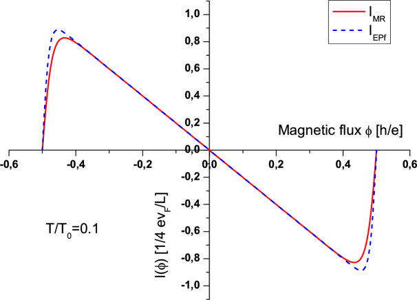
Figure 1: Persistent currents in the MR and EPf states computed numerically for $T/T_{0}=0.1$. The flux is measured in units $h/e$ and the current’s unit is $ev_{F}/4L$. The period is 1 flux quantum for both states and the amplitudes are $I_{\mathrm{MR}}^{\max}=0.828$ and $I_{\mathrm{EPf}}^{\max}=0.887$.

indicate that both currents are periodic in $\phi$ with period exactly $1$. We do not see any anomalous oscillations, such as half-flux periodicity of the persistent currents [38, 40], which is characteristic for the BCS paired condensates, or more generally for some broken symmetries, neither in the MR nor in the EPf states for all temperatures $0.05\leq T/T_{0}\leq 9$ that we could access numerically. This is exactly the content of the Bloch theorem, which is also known as the Byers–Yang theorem [22] in the context of superconductors.

The amplitudes of the persistent currents in the EPf and MR states decay exponentially with temperature, as shown in Fig. 2.

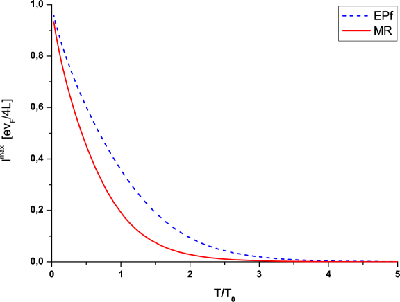
Figure 2: Temperature decay of the persistent current’s amplitudes in the MR and EPf states. The amplitude are computed numerically in units $ev_{F}/4L$, the temperature is measured in units of $T_{0}$.

While at $T=0$ both currents have the same amplitude $I^{\max}_{\mathrm{MR}}=I^{\max}_{\mathrm{EPf}}$, for finite temperature the amplitude of the current $I_{\mathrm{EPf}}$ is always bigger than that of $I_{\mathrm{MR}}$. This fact could be used to detect (e.g., in a SQUID experiment) any transition between the two states. For convenience we also show on Fig. 3 the logarithmic plot of the temperature decay Fig. 2 of the persistent currents’ amplitudes. The temperature dependence on Fig. 3 is not linear, showing two distinct regions, which we shall conventionally call low-temperature and high-temperature regions and shall investigate separately. This suggests the existence of two different mechanisms reducing the amplitude of the persistent currents at finite temperature.

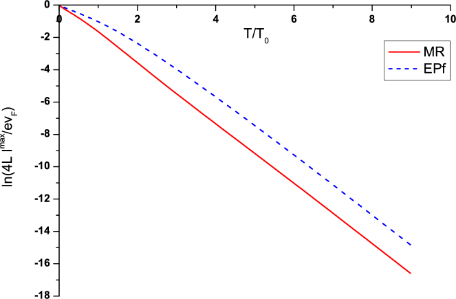
Figure 3: Logarithmic plot of the temperature dependence of the amplitudes of the persistent currents (in units of $ev_{F}/4L$) in the MR and EPf states computed numerically for temperatures $0.05\leq T/T_{0}\leq 9$

We recall that the chiral persistent currents computed here are universal in the sense that due to the absence of backscattering from impurities, there is no reduction from weak disorder [41] (for FQH states without simultaneously counter-propagating modes [42]).

8.1 Low temperature limit

In the low temperature limit $T/T_{0}\to 0$ the modular parameter vanishes, $q=\mathrm{e}^{-2\pi^{2}\frac{T_{0}}{T}}\to 0$, and the low temperature asymptotics of the persistent current is determined by the leading term, coming from the vacuum sector, which is proportional to $q^{0}$ , multiplied by the CZ factor (10). Therefore the partition functions in the EPf and MR states are the asymptotically same in this limit

$$Z^{+}_{\mathrm{EPf}}(T,\phi)=Z^{+}_{\mathrm{MR}}(T,\phi)\mathop{\simeq}\limits_{T/T_{0}\to 0}\exp\left(-\frac{\pi^{2}}{2}\frac{T_{0}}{T}\phi^{2}\right).$$

and the zero-temperature amplitudes of the persistent currents in the EPf and MR states are given by (without the contribution from the lowest Landau level)

$$I^{\max}_{\mathrm{EPf}}=I^{\max}_{\mathrm{MR}}=\frac{1}{4}\frac{ev_{F}}{L}\quad\mathrm{for}\quad T=0.$$ (30)

Note that in general there is a large, non-mesoscopic contribution to the zero temperature amplitude of the current [42], which is proportional to the cyclotron frequency $\omega_{c}$, hence slowly varying with $B$ (see Eq. (37) in [37]). This component of the persistent current cannot be derived within the CFT approach because the latter is only a theory of the low-lying excitations above the ground state, while the $\omega_{c}$ contribution reflects the properties of the ground state, and involves states deep below the Fermi energy [42]. Nevertheless, the oscillating part of the persistent currents derived here seems to be measurable in SQUID experiments [25].

Taking into account also the next-to-leading order contribution to the mesoscopic persistent current $I(T,\phi)$ and finding its maximum for $T$-fixed gives the following low-temperature asymptotics for the current’s amplitude in the EPf state (see Appendix C for details)

$$I^{\max}_{\mathrm{EPf}}(T) \quad\mathop{\simeq}\limits_{T/T_{0}<<1}\quad \frac{ev_{F}}{L}\frac{1}{2\pi^{2}}\frac{T}{T_{0}}\mathrm{arccosh}\left(\frac{1}{2\pi^{2}}\frac{T}{T_{0}}\exp\left(\frac{\pi^{2}}{2}\frac{T_{0}}{T}\right)\right)-$$ (31)

$$\quad-\quad \frac{ev_{F}}{L}\left[\left(\frac{1}{2\pi^{2}}\right)^{2}\left(\frac{T}{T_{0}}\right)^{2}-\exp\left(-\pi^{2}\frac{T_{0}}{T}\right)\right]^{1/2}$$

and

$$I^{\max}_{\mathrm{MR}}(T) \quad\mathop{\simeq}\limits_{T/T_{0}<<1}\quad \frac{ev_{F}}{L}\frac{1}{\pi^{2}}\frac{T}{T_{0}}\mathrm{arccosh}\left(\frac{2}{\pi^{2}}\frac{T}{T_{0}}\exp\left(\frac{\pi^{2}}{4}\frac{T_{0}}{T}\right)\right)-$$ (32)

$$\quad-\quad \frac{1}{2}\frac{ev_{F}}{L}\left[\left(\frac{2}{\pi^{2}}\right)^{2}\left(\frac{T}{T_{0}}\right)^{2}-\exp\left(-\frac{\pi^{2}}{2}\frac{T_{0}}{T}\right)\right]^{1/2}$$

for that in the MR state. The low-temperature region, corresponding to $0\leq T/T_{0}\leq 0.3$, is shown separately on Fig. 4.

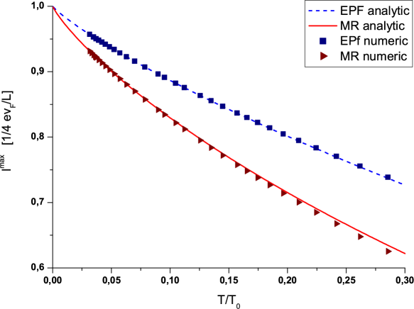
Figure 4: Low-temperature dependence of the persistent currents’ amplitudes in the MR and EPf states computed numerically for $0.05\leq T/T_{0}\leq 0.3$ and analytically, using Eqs. (31) and (32), for $0\leq T/T_{0}\leq 0.3$.

We note that, according to Fig. 4, the asymptotic formulae (31) and (32) give excellent approximations for $T/T_{0}\leq 0.1$.

The mechanism responsible for this decay [25] is the mixing of contributions of energy levels in an energy interval $k_{B}T$, which reduces the current since adjacent levels give opposite contributions. The characteristic scale for this mixing is given by the energy gap (not simply by the level spacing $\hbar\ 2\pi v_{F}/L$).

8.2 High temperature limit

The high-temperature limit $T/T_{0}\to\infty$ is a non-trivial one since $q=\mathrm{e}^{-2\pi^{2}\frac{T_{0}}{T}}\to 1$ is at the border of the convergence interval for the partition functions. However, since the latter is constructed as a sum of RCFT characters, one could use their $S$-covariance to relate the high-temperature and low-temperature limits (in proper modular parameters). Note that, unlike the annulus partition functions, the disk partition functions (27) and (28) are not $S$-invariant and as we shall see this leads to a completely different temperature behaviour after $S$-transformation. We find that the amplitudes of the persistent currents in the EPf and MR states decay exponentially with the temperature (see Appendix D for details) for $T/T_{0}>>1$, i.e.,

$$I^{\max}_{\mathrm{EPf}}(T)\quad\mathop{\simeq}\limits_{T/T_{0}>>1}\quad\frac{2}{\pi}\frac{ev_{F}}{L}\left(\frac{T}{T_{0}}\right)\exp\left(-2\frac{T}{T_{0}}\right)$$ (33)

$$I^{\max}_{\mathrm{MR}}(T)\quad\mathop{\simeq}\limits_{T/T_{0}>>1}\quad\frac{2}{\pi}\frac{ev_{F}}{L}\left(\frac{\sqrt{2}-1}{\sqrt{2}+1}\right)\left(\frac{T}{T_{0}}\right)\exp\left(-2\frac{T}{T_{0}}\right)$$ (34)

The logarithmic plots of the amplitudes of the persistent currents in the EPf and MR states, computed numerically, in the high-temperature region, corresponding to $1\leq T/T_{0}\leq 9$ which are given in Fig. 3 become almost linear, with the same slopes but different $y$-intercepts. After removing the subleading $\ln(T/T_{0})$ contribution, which is explicit in Eqs. (33) and (34), the Least-Squares fit gives $-2.00005$ for the slope in the EPf state and $-2.004$ for that in the MR state, while the $y$-intercepts give amplitudes (in units $ev_{F}/4L$) $2.547$ for the EPf and $0.452$ for the MR states respectively. Again, we see that the high-temperature asymptotic formulae (33) and (34) are in excellent agreement with the numerical calculations shown in Fig. 3. The ratio $I^{\max}_{\mathrm{EPf}}/I^{\max}_{\mathrm{MR}}$ increases to $5.813$ for $T/T_{0}\to 9$, which is very close to the analytic value $(\sqrt{2}+1)/(\sqrt{2}-1)\simeq 5.828$, that gives the universal ratio for $T/T_{0}\to\infty$.

This high-temperature universal non-Fermi liquid behaviour, characterized by the temperature $T_{0}$, which is closely related to the level spacing, expresses another mechanism for “thermal smearing” [42] of the persistent currents.

9 Phase transition between the EPf and MR states

Although continuous symmetries in (1+1) D cannot be spontaneously broken [43], there could be a spontaneous breaking of some discrete symmetry at finite temperature $T_{c}>0$. As we have shown in Sect. 5 the ${\mathbb{Z}}_{2}$ fermion parity is spontaneously broken in the R-sector of the Ising model. Therefore we believe that there is a classical II-nd order phase transition, at $\nu=5/2$, which is characterized by the spontaneous breaking of this ${\mathbb{Z}}_{2}$ symmetry. The high temperature “symmetric” phase ($T>T_{c}$) corresponds to the EPf state, in which the chiral fermion parity is well-defined, while in the low temperature “ordered” phase ($T<T_{c}$), corresponding to the MR state, this symmetry is spontaneously broken. This is different from the spontaneous magnetization in the 2D Ising model where the ${\mathbb{Z}}_{2}$ symmetry changes the sign of the spin field $\sigma\to-\sigma$, while leaving the fermion invariant. In the present case the generator $\gamma_{F}$ of the symmetry anticommutes with the fermion $\varphi(z)$ and the “order parameter”, which is given by the vacuum expectation value $\langle\varphi(\theta)\rangle_{\mathrm{PBC}}$ in the sector with periodic boundary conditions on the cylinder, is fermionic and hence not directly observable. Nevertheless it has crucial implications for the corresponding phases, such as change of the ground state energy and spectrum of excitations on the cylinder and diamagnetic/paramagnetic ground state’s structure depending on the fermion parity.

The nature of this phase transition is not clear despite the extensive numerical work [4, 14]. Motivated by the analysis of the chiral fermion parity, we propose the following scenario: as temperature increases the system undergoes a II-nd order phase transition, from the MR state, in which the chiral fermion parity is spontaneously broken, to an intermediate compressible Composite Fermions (CF) Fermi liquid state found before [4, 14, 24], which possesses this ${\mathbb{Z}}_{2}$ symmetry, and then a I-st order phase transition from the CF state to the EPf one. Since the resistance $R_{0}$ in Fig. 6 has a jump, one would expect that the transition MR $\to$ EPf is simply of first order. However, according to our analysis, this transition is accompanied by spontaneous breaking of the ${\mathbb{Z}}_{2}$ chiral fermion parity symmetry discussed in Sect. 5. On the other hand, a second order transition between the EPf and the MR states, with spontaneous breaking of the fermion parity, cannot occur directly since incompressible Hall states with different topological orders, such as the MR and the EPf states, support residual neutral gapless modes at the phase boundary, leading to a first order transition [44, 45]. However, there is a possibility for a two-step process involving an intermediate compressible state [44, 45]. In that case, as temperature decreases, the EPf state undergoes a first order phase transition to the CF Fermi liquid state, in which the ${\mathbb{Z}}_{2}$ symmetry is preserved, and then a second order phase transition to the MR state in which the ${\mathbb{Z}}_{2}$ symmetry is broken.

Note that, unlike the MR state, the compressible CF state[14] is ${\mathbb{Z}}_{2}$ symmetric and, at the same time (despite its compressibility) has the topological structure similar to that of the MR state. Indeed, as pointed out in [14], the $4$ values of the total momentum $\bf{K}$ ($3$ distinct values) correspond to the $3$ distinct values of $\bf{K}$ in the MR state on the torus. In fact, the CF state has the topological structure of the 331 state, which possesses this ${\mathbb{Z}}_{2}$ symmetry, see Sect. 5. Therefore we believe that the transition MR $\to$ CF is in the same universality class as the transition 331 $\to$ MR and is characterized by the spontaneous breaking of the chiral fermion parity. We stress that due to the similar topological structure of the MR and CF states, the phase boundary between these phases do not support gapless neutral modes [44], which opens the possibility of a second order transition, in which the fermion parity is spontaneously broken. On the other hand, because of the topological mismatch, the transition from the CF to the EPf state could only be of first order. This scenario is in agreement with the numerical calculations [4, 14] as well as with the activation experiment at $\nu=5/2$, see Fig. 3 in [2], where a “kink” was observed around $T=15$ mK.

In Fig. 5 we plot the low-temperature behaviour of the free energy on the edge as computed numerically from the CFT.

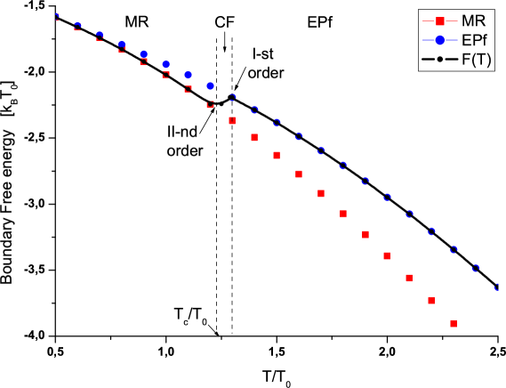
Figure 5: Boundary free energy for the MR and EPf states at low temperature computed numerically from CFT (without additional flux, i.e., $\phi=0$). The free energy for the intermediate compressible phase, between the two vertical dashed lines, is qualitative. The black line shows the expected behaviour of the free energy $F(T)$ for $\nu=5/2$.

We stress that the CFT description of the FQH system is valid as long as the system is incompressible, i.e., for temperatures well below the activation energy. Note that the CFT dimension, which is equal to the average spin [18], is proportional to the (ideal) average quasiparticle–quasihole energy [18], i.e., the activation energy is a half of the gap computed in Eq. (18) and Eq. (19). Therefore in systems such as the $\nu=5/2$, with more than one phases with different gaps, there might be an interesting interplay between the various phases at different temperatures. As can be seen from Fig. 5, the free energy of the MR state is always lower than that of the EPf and we believe that the FQH system is in the MR phase for temperature $T<\Delta_{\mathrm{MR}}/2k_{B}$, i.e., until the free energy for the MR state computed from the CFT is a good approximation. This is confirmed by numerical calculations at zero temperature [14]. The free energy for the MR and EPf states at zero temperature are the same, i.e., $F_{\mathrm{MR}}(T=0)=F_{\mathrm{EPf}}(T=0)$, as it should be since both phases share the same absolute ground state. For temperature higher than the MR activation energy $T>\Delta_{\mathrm{MR}}/2k_{B}$, the boundary free energy goes very fast to its value at zero temperature (the ground state energy) since the lowest-energy charged edge excitations are quickly transferred into the bulk where they have less momentum and hence less energy as compared to the edge. This may lead to a II-nd order phase transition, at critical temperature $T_{c}\simeq\Delta_{\mathrm{MR}}/2k_{B}$ characterized by the energy gap in the MR state, from the MR state to a compressible state, which seems to be topologically equivalent to the CF Fermi liquid state. Then, for temperature very close to $T_{c}$, the free energy of the intermediate phase CF crosses the free energy of the EPf state leading to a I-st order phase transition CF $\to$ EPf as shown in Fig. 5. This is consistent with the experimental observation of the change in the slope of $\ln(R_{xx})$, which looks like a single transition. The characteristic temperature for this two-step transition in the absence of disorder could be estimated using the gap ansatz (17) with $\Delta_{\mathrm{q.h.}}^{\mathrm{MR}}=1/8$ for $\Gamma=0$ and $\alpha$ being the ratio of the level spacing and Coulomb energy, to be

$$T_{c}=\frac{\Delta_{\mathrm{MR}}}{2k_{B}}=\pi^{2}T_{0}\Delta_{\mathrm{q.h.}}^{\mathrm{MR}}=\frac{1}{2}\hbar\frac{2\pi v_{F}}{L}\Delta_{\mathrm{q.h.}}^{\mathrm{MR}}\quad\Longrightarrow\quad\frac{T_{c}}{T_{0}}=\frac{\pi^{2}}{8}.$$ (35)

The different gaps, Eqs. (18) and (19) for the sample of [2], in both phases lead to a change of the slope in the logarithmic plot of the diagonal resistance $R_{xx}=R_{0}\exp(-\Delta/2k_{B}T)$, as a function of $1/T$, in the thermal activation experiment, which is illustrated on Fig. 6.

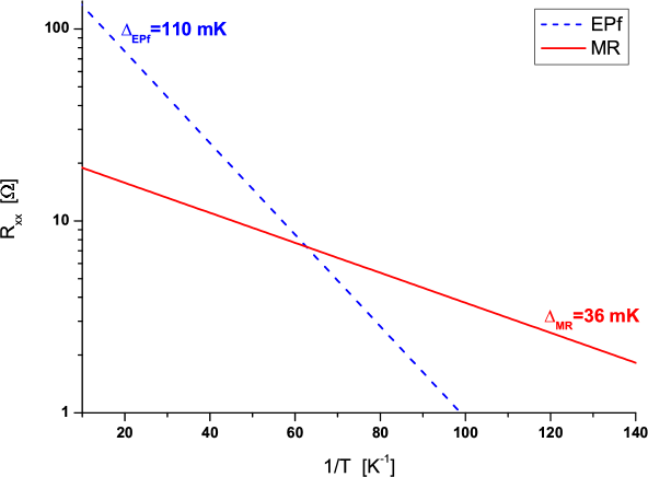
Figure 6: Logarithmic plot of the longitudinal resistance in the MR and EPf states as a function of the inverse temperature. The slopes (i.e., the gaps) for both states correspond to the sample of [2] and the change of the slope is an indication of a phase transition

The trial values of $R_{0}^{\mathrm{EPf}}=230\Omega$, $\Delta_{\mathrm{MR}}=36$mK and $R_{0}^{\mathrm{EPf}}/R_{0}^{\mathrm{MR}}\simeq 10.2$, which were used to plot Fig. 6, have been chosen for maximal overlap with Fig. 3 in [2]. Our fit shows that the temperature at which the two lines $\ln R_{xx}^{\mathrm{EPf}}=\ln R_{0}^{\mathrm{EPf}}-\Delta_{\mathrm{EPf}}/2k_{B}T$ and $\ln R_{xx}^{\mathrm{MR}}=\ln R_{0}^{\mathrm{MR}}-\Delta_{\mathrm{MR}}/2k_{B}T$ intersect is not exactly $T=\Delta_{\mathrm{MR}}/2k_{B}\simeq 18$mK but rather $T=\Delta_{\mathrm{MR}}/2k_{B}-\delta T$, where the shift $\delta T$ is determined from

$$\frac{R_{0}^{\mathrm{EPf}}}{R_{0}^{\mathrm{MR}}}=\exp\left(\frac{\Delta_{\mathrm{EPf}}-\Delta_{\mathrm{MR}}}{\Delta_{\mathrm{MR}}-2\delta T}\right)\simeq 10.2\quad\Longrightarrow\quad\delta T\simeq 2\mathrm{mK}.$$

This might be an indication that the transition MR $\to$ EPF is not simply of I-st order, but involves an intermediate state. When the residual disorder is taken into account, the critical temperature (35) is supposed to decrease in the same way like the energy gap [18]. For example, our scenario implies for the sample of [2], where $\Delta_{\mathrm{MR}}\simeq 36$ mK, that $T_{c}\simeq 16$ mK and for $T<T_{c}$ (i.e., for $1/T>62$) the system is in the MR phase, for $16<T<18$ mK ($55<1/T<62$) it is in the CF phase, while for $18<T<55$ mK ($20<1/T<55$) it is in the EPf phase, as illustrated on Fig. 5 for a pure FQH system.

Here we have to stress that the analysis based on the boundary free energy is incomplete since we do not account for the contribution from the bulk. Nevertheless, the CFT free energy carries information about the universal properties of the system, so that it could label the FQH universality classes, and we believe its behaviour could capture any transition between different FQH phases.

A similar two-step II-nd order phase transition has been proposed for the $\nu=4/3$ plateau [45]. In that case there seems to exist an intermediate metallic state which opens the possibility of a two-step transition similar to that described above, i.e., a II-nd order transition from the spin-polarized to the intermediate partially polarized compressible phase and then a II-nd order transition to the spin-polarized state. This is to be compared with the situation of the $\nu=2/3$ plateau where all transitions are I-st order [45, 44] since a compressible state does not exist and because usually II-nd order phase transitions are accompanied by discontinuity in the compressibility, i.e., any direct transition between incompressible states, even if both states have the same topological structure, is most likely not of II-nd order. For $\nu=2/3$, where the PH-conjugate of the $\nu=1/3$ Laughlin state and the spin-singlet state seem to have the same topological structure, it is confirmed by numerical calculations [44] that the transition is of I-st order.

The phase transitions described above seem to be “classical” as they occur at non-zero temperature. That is probably why in the numerical calculations [14], performed at $T=0$, they only see a second order phase transition MR $\to$ CF and say nothing about any other transition, such as CF $\to$ EPf. Finally, we stress that although we believe that the transition MR $\to$ CF is of II-nd order, there is still a possibility for a smooth crossover MR $\to$ CF [14], however, the transition CF $\to$ EPf is most likely of I-st order.

10 Abelian versus non-abelian statistics

The phase transition discussed in the previous section is actually a classical transition between abelian and non-abelian FQH states. It seems that non-abelian statistics is preferred at low temperature, while at higher temperature the abelian states are more favorable. Perhaps, this is characteristic for all FQH plateaux for which abelian and non-abelian states are competing. For instance, at $\nu=7/3$ and $8/3$ there exist (PH conjugated) $k=1$ Laughlin states and $k=4$ parafermion states, the latter being non-abelian. Probably, such phase transitions can explain as well the sharp kinks observed in the activated experiment for these plateaux [2]. Note that, e.g. for $\nu=7/3$, the phase transition between the high-temperature abelian phase (the Laughlin state) and the low-temperature non-abelian phase (the Read–Rezayi state) is of first order, again because of the different topological orders [44], the absence of an intermediate compressible state and the fact that there is no symmetry, which can be spontaneously broken. This is in agreement with the sharp change of the slope and the $y$-intercept of the diagonal resistance in the activation experiment [2] and is reminiscent of the first order phase transition between the spin-singlet and the spin-polarized states at $\nu=2/3$ [44, 45] which was discussed at the end of the previous section.

11 Conclusions

We have described a new universality class relevant for the FQH state at $\nu=5/2$, determined by the rational CFT of the abelian EPf state, which has a well-defined chiral fermion parity number and could be viewed as a ${\mathbb{Z}}_{2}$ supersymmetric extension of the MR state. Using our previous analysis [18] we have computed the energy gaps, Eqs. (18) and (19) for the EPf and MR states, as well as the periods and amplitudes of the persistent currents in both states for a disk sample. Based on our analysis we conclude that there might be a two-step phase transition between the MR and EPf states at finite temperature, involving an intermediate compressible state, in which the chiral fermion parity symmetry is spontaneously broken.

In order to reveal the nature of the FQH state at $\nu=5/2$ new and more precise experiments are needed. The phase transition MR $\to$ EPf investigated in this paper could be detected by measuring several quantities for temperature in the range $10$ mK $\leq T\leq 30$ mK:

• Quasiparticle charges:
  The (minimal) quasiparticle charge in both states is different: $Q_{\mathrm{q.h.}}=1/4$ for the MR state and $Q_{\mathrm{q.h.}}=1/2$ for the EPf state. Therefore, a charge-measuring experiment, such as shot-noise, for temperatures in the above range could confirm whether the phase transition seen in the activation experiment [2] is the transition between the MR and EPf states described in this paper.
  

• Energy gaps:
  The activation energy of the EPf state is significantly bigger than that of the MR state, i.e., $\Delta_{\mathrm{EPf}}\sim 3\Delta_{\mathrm{MR}}$ for the sample of [2]. Thus, a more precise activation experiment for a high-mobility sample like that of [2] in the above range could confirm our predictions about the energy gaps and the phase transition.
  

• Persistent currents:
  The ratio of the amplitudes of the persistent currents in the EPf and MR states at a transition temperature $T_{c}/T_{0}\sim 1.23$ is $I^{\mathrm{EPf}}/I^{\mathrm{MR}}\sim 2.15$. However, when we take into account the (same) contribution from the two $\nu=1$ lowest Landau levels (filled completely with electrons of opposite spin), which is estimated to be $2\times 1.07$ in our units $ev_{F}/4L$, this ratio decreases to $1.06$, which is not detectable with the current SQUID precision [25]. Nevertheless, we believe that when the precision becomes better than $5\%$, the phase transition between the two phases could be practically detected in a high-mobility sample similar to that of [2].

In addition, there might be a phase transition at zero temperature to a BCS-type condensate but that universality class would be different from both the MR and the EPf states according to Fig. 1, since the periodicity of the persistent current in the condensate is expected to be $1/2$ of the flux unit, while that of the MR and EPf states is always $1$. Probably, this is described by the strong pairing phase of [8, 14].

Finally, we believe that all these new experiments, as well as the analysis in this paper, may shed more light on the nature of the mysterious FQH state at $\nu=5/2$. One important aspect of the results presented in this paper is the anticipation that the non-abelian quasiparticles can be observed in practice only for temperatures below the transition temperature, which we estimate as $T_{c}\sim 15$ mK for $\nu=5/2$ in the sample of [2].

Appendix A Weak modular invariance of the EPf state

In this appendix we are going to show that the characters of the EPf state are modular covariant, i.e., they belong to a $2$ dimensional representation of the subgroup [29, 10] $\Gamma_{\theta}\subset PSL(2,{\mathbb{Z}})$ of the modular group. We use the explicit form of the modular $S$-matrix for the Ising model, in the basis of characters $(\mathrm{ch}_{i})=(\mathrm{ch}_{0},\mathrm{ch}_{1/16},\mathrm{ch}_{1/2})$,

$$S=\frac{1}{2}\left[\begin{array}[]{rrr}1&\sqrt{2}&1\cr\sqrt{2}&0&-\sqrt{2}\cr 1&-\sqrt{2}&1\end{array}\right],\quad\mathrm{where}\quad\mathrm{ch}_{i}\left(-\frac{1}{\tau}\right)=\sum_{j=1}^{3}\,S_{ij}\,\mathrm{ch}_{j}(\tau)$$

to show that the Ising factor in the characters (15) is $S$-invariant, i.e.,

$$\mathrm{ch}_{0}\left(-\frac{1}{\tau}\right)+\mathrm{ch}_{1/2}\left(-\frac{1}{\tau}\right)=\mathrm{ch}_{0}(\tau)+\mathrm{ch}_{1/2}(\tau).$$ (36)

On the other hand, this combination is $T^{2}$-invariant ($\tau\to\tau+2$) up to a phase, i.e.,

$$\left|\mathrm{ch}_{0}(\tau+2)+\mathrm{ch}_{1/2}(\tau+2)\right|^{2}=\left|\mathrm{ch}_{0}(\tau)+\mathrm{ch}_{1/2}(\tau)\right|^{2},$$

while not being simply $T$-invariant since $|\mathrm{ch}_{0}(\tau+1)+\mathrm{ch}_{1/2}(\tau+1)|^{2}=|\mathrm{ch}_{0}(\tau)-\mathrm{ch}_{1/2}(\tau)|^{2}$. We recall that the Ising characters are neutral and therefore the $U:\zeta\to\zeta+1$ and $V:\zeta\to\zeta+\tau$ transformations do not change them. Thus, the Ising part of the characters is invariant with respect to $T^{2},S,U,V$ transformations and therefore the complete characters (15) of the EPf state have the transformation properties of the bosonic $\nu=1/2$ Laughlin state [29] with respect to these transformations.

Appendix B Equivalence of the persistent currents of the EPf state and the bosonic $\nu=1/2$ Laughlin state

According to Eq. (29) the neutral factor in Eq. (27), coming from the Ising model, does not contribute to the persistent current of the EPf state. The latter can be computed by substituting $\zeta\to\zeta+\phi\tau$, like in Eq. (29) and using the transformation property of the $K$-functions (2)

$$\mathrm{e}^{-\frac{\pi}{m}\frac{\left(\mathrm{Im}\ (\zeta+\phi\tau)\right)^{2}}{\mathrm{Im}\ \tau}}K_{l}(\tau,\zeta+\phi\tau;m)=\mathrm{e}^{-\frac{2\pi i}{m}\left(\frac{\phi^{2}}{2}\mathrm{Re}\ \tau+\phi\mathrm{Re}\ \zeta\right)}\left(\mathrm{e}^{-\frac{\pi}{m}\frac{(\mathrm{Im}\ \zeta)^{2}}{\mathrm{Im}\ \tau}}K_{l+\phi}(\tau,\zeta;m)\right).$$ (37)

In addition one could express the chiral partition function (26) for the $\nu=1/m$ Laughlin state as

$$Z^{+}_{\mathrm{Laugh}}(\tau,\zeta)=\mathrm{e}^{-\frac{\pi}{m}\frac{(\mathrm{Im}\ \zeta)^{2}}{\mathrm{Im}\ \tau}}\sum_{l\;\mathrm{mod}\;m}K_{l}(\tau,\zeta;m)=\mathrm{e}^{-\frac{\pi}{m}\frac{(\mathrm{Im}\ \zeta)^{2}}{\mathrm{Im}\ \tau}}K_{0}(\tau,\zeta/m;1/m).$$

Applying Eq. (37) to the above equation and ignoring the $\zeta$-independent $\eta$ functions in Eq. (2), we get that the non-zero contribution to the persistent current for the $\nu=1/m$ Laughlin state comes from

$$K_{\phi/m}(\tau,0;1/m)\sim\sum_{n\in{\mathbb{Z}}}q^{\frac{1}{2}\frac{1}{m}(n+\phi)^{2}}=\sum_{n\in{\mathbb{Z}}}\mathrm{e}^{-\frac{\pi^{2}}{m}\frac{T_{0}}{T}(n+\phi)^{2}},$$ (38)

which coincides with Eq. (38) in [37] up to the sign of $\phi$, that can be changed by a substitution $n\to-n$. Therefore, the persistent current for the EPf state is the same as that for the $\nu=1/2$ Laughlin state.

Appendix C Low-temperature asymptotics of the persistent currents

For $T/T_{0}\to 0$ the modular parameter vanishes, $q=\exp\left(-2\pi^{2}T_{0}/T\right)\to 0$, so it is sufficient to keep only the first three terms $n=0,\pm 1$ in Eq. (38). Thus, for the persistent current in the EPf state one gets

$$I_{\mathrm{EPf}}(T,\phi)=-\frac{1}{2}\frac{ev_{F}}{L}\phi+2\exp\left(-\frac{\pi^{2}}{2}\frac{T_{0}}{T}\right)\sinh\left(\pi^{2}\frac{T_{0}}{T}\phi\right),\quad\frac{T}{T_{0}}<<1,$$ (39)

for $|\phi|\leq\frac{1}{2}$. The local maximum for $-1/2\leq\phi\leq 1/2$ at fixed temperature is located at

$$\phi^{\max}_{\mathrm{EPf}}(T)=-\frac{1}{\pi^{2}}\frac{T}{T_{0}}\mathrm{arccosh}\left(\frac{1}{2\pi^{2}}\frac{T}{T_{0}}\exp\left(\frac{\pi^{2}}{2}\frac{T_{0}}{T}\right)\right).$$ (40)

Substituting Eq. (40) into Eq. (39) and using the identity $\sinh(\alpha)=\mathrm{sgn}\ (\alpha)\sqrt{\cosh^{2}(\alpha)-1}$ we obtain Eq. (31). The same procedure applied to the MR state gives Eq. (32).

Appendix D High-temperature asymptotics of the persistent currents

The high-temperature limit $T/T_{0}\to\infty$ is not so trivial because the modular parameter $q=\exp\left(-2\pi^{2}T_{0}/T\right)\to 1$ is at the border of the convergency interval for the partition functions. Therefore it is more convenient to perform $S$ transformation first

$$S:\begin{array}[]{l}\tau=-1/\tau^{\prime}\\ \zeta=-\zeta^{\prime}/\tau^{\prime}\end{array}\quad{\Longleftrightarrow}\quad\begin{array}[]{l}\tau^{\prime}=-1/\tau=iT/\pi T_{0}\\ \zeta^{\prime}=\zeta/\tau=\phi\end{array}.$$ (41)

Now the modular parameter $q^{\prime}=\mathrm{e}^{2\pi i\tau^{\prime}}=\exp\left(-2T/T_{0}\right)\to 0$ when $T/T_{0}\to\infty$. Here we use the transformation properties of the characters for the Laughlin FQH state with $\nu=1/m$ [29]

$$\chi_{l}(\tau,\zeta)=\exp\left(i\frac{\pi}{m}\mathrm{Re}\ \frac{{\zeta^{\prime}}^{2}}{\tau^{\prime}}\right)\sum\limits_{l^{\prime}=0}^{m-1}S_{ll^{\prime}}\ \chi_{l^{\prime}}(\tau^{\prime},\zeta^{\prime}),\quad S_{ll^{\prime}}=\frac{1}{\sqrt{m}}\exp\left(-2\pi i\ \frac{ll^{\prime}}{m}\right).$$ (42)

Note that $\mathrm{Re}\ {\zeta^{\prime}}^{2}/\tau^{\prime}=\phi^{2}\mathrm{Re}\ (1/\tau^{\prime})=0$. Next, substitute Eq. (42) into Eq. (26) to get

$$Z^{+}_{\mathrm{EPf}}(T,\phi)=\sum_{l^{\prime}=0}^{m-1}\chi_{l^{\prime}}(\tau^{\prime},\zeta^{\prime})\sum_{l=0}^{m-1}S_{ll^{\prime}}=\sqrt{m}\ \chi_{0}(\tau^{\prime},\zeta^{\prime}),$$

where we have used that $\sum_{l=0}^{m-1}S_{ll^{\prime}}=\sqrt{m}\delta_{l,0}\;\mathrm{mod}\;m$. Now (ignoring $\sqrt{m}$ and the $\eta$-function) keeping only the leading three terms $n=0,\pm 1$ in $\chi_{0}(\tau^{\prime},\zeta^{\prime})$ and taking into account that $\mathrm{Im}\ \zeta^{\prime}=\mathrm{Im}\ \phi=0$, i.e., the CZ factors are trivial, we get

$$\ln Z^{+}_{\mathrm{EPf}}(T,\phi)\quad\mathop{\simeq}\limits_{T/T_{0}>>1}\quad\ln\left(1+2\cos(2\pi\phi)\exp\left(-m\frac{T}{T_{0}}\right)\right).$$ (43)

The second term is very small in this limit and we use $\ln(1+x)\simeq x$ valid for $x<<1$ to get, after differentiation with respect to $\phi$ at $\phi^{\max}=-1/4$, Eq. (33) for $m=2$. Note that the same result can be obtained from the $\theta_{3}$ function formula Eq. (39) in Ref. [37] . Indeed, for $T/T_{0}>>1$ we have $\sinh(nmT/T_{0})^{-1}\simeq 2\exp(-nmT/T_{0})$. Then keeping only the first term, $n=1$ in Eq. (39) in [37], we arrive at the analog of our Eq. (33) for general $m$.

We repeat the same calculation for the MR state using the $S$-matrix computed in [7] (see Eq. (5.8) there). The difference is that now

$$\sum_{l=0,\pm 1,\pm 2,4}S_{ll^{\prime}}=\left\{\begin{array}[]{ll}\sqrt{2}+1,&\quad\mathrm{for}\quad l^{\prime}=0\\ 0,&\quad\mathrm{for}\quad l^{\prime}=\pm 1,\pm 2\\ \sqrt{2}-1,&\quad\mathrm{for}\quad l^{\prime}=4\end{array}\right.$$

so that

$$Z^{+}_{\mathrm{MR}}(T,\phi)=\left(\chi_{0}(\tau^{\prime},\zeta^{\prime})-\chi_{4}(\tau^{\prime},\zeta^{\prime})\right)+\sqrt{2}\left(\chi_{0}(\tau^{\prime},\zeta^{\prime})+\chi_{4}(\tau^{\prime},\zeta^{\prime})\right).$$

Next we use that for $q^{\prime}\to 0$ the Ising model characters satisfy $\mathrm{ch}_{0}(\tau^{\prime})\pm\mathrm{ch}_{1/2}(\tau^{\prime})\to\mathrm{ch}_{0}(\tau^{\prime})$ and the identity

$$K_{2l}(\tau,2\zeta;8)\pm K_{2l+4}(\tau,2\zeta;8)=K^{\pm}_{l}(\tau,\zeta;2)=$$

$$=\frac{1}{\eta(\tau)}\sum_{n\in{\mathbb{Z}}}(\pm 1)^{n}q^{(n+l/2)^{2}}\mathrm{e}^{2\pi i\zeta(n+l/2)}$$ (44)

to get

$$Z^{+}_{\mathrm{MR}}(T,\phi)\quad\mathop{\simeq}\limits_{T/T_{0}>>1}\quad\left(K^{-}_{0}(\tau^{\prime},\zeta^{\prime};2)+\sqrt{2}K^{+}_{0}(\tau^{\prime},\zeta^{\prime};2)\right)\mathrm{ch}_{0}(\tau^{\prime}),$$

which after dropping $\zeta^{\prime}$ independent factors gives

$$\ln Z^{+}_{\mathrm{MR}}(T,\phi)\quad\mathop{\simeq}\limits_{T/T_{0}>>1}\quad\ln\left(1+\frac{\sqrt{2}-1}{\sqrt{2}+1}2\cos(2\pi\phi)\exp\left(-2\frac{T}{T_{0}}\right)\right).$$

Again we use $\ln(1+x)\simeq x$, $x<<1$ and differentiate this equation with respect to $\phi$ at $\phi^{\max}=-1/4$, which gives the high-temperature asymptotics (34) of the persistent current in the MR state.

References

- [1] R. Willett, J. P. Eisenstein, H. L. Störmer, D. C. Tsui, A. C. Gossard, and J. H. English, “Observation of an even-denominator quantum number in the fractional quantum Hall effect,” Phys. Rev. Lett. 59 (1987) 1776.
- [2] W. Pan, J.-S. Xia, V. Shvarts, D. E. Adams, H. L. Störmer, D. C. Tsui, L. N. Pfeiffer, K. W. Baldwin, and K. W. West, “Exact quantization of the even-denominator fractional quantum Hall state at Landau level filling factor,” Phys. Rev. Lett. 83 (1999) 3530.
- [3] J. Eisenstein, R. Willett, H. L. Störmer, D. C. Tsui, A. C. Gossard, and J. H. English, “Collapse of the even-denominator fractional quantum Hall effect in tilted fields,” Phys. Rev. Lett. 61 (1988) 997.
- [4] R. Morf, “Transition from quantum Hall to compressible states in the second landau level: new light on the =5/2 enigma,” Phys. Rev. Lett. 80 (1998) 1505, cond-mat/9809024.
- [5] W. Pan, H. L. Störmer, D. C. Tsui, L. N. Pfeiffer, K. W. Baldwin, and K. W. West, “Experimental evidence for a spin-polarized ground state in the fractional quantum Hall effect,” (2001) cond-mat/0103144.
- [6] F. Haldane and E. Rezayi Phys. Rev. Lett. 60 (1988) 956.
- [7] A. Cappelli, L. S. Georgiev, and I. T. Todorov, “A unified conformal field theory description of paired quantum Hall states,” Commun. Math. Phys. 205 (1999) 657, hep-th/9810105.
- [8] N. Read and D. Green, “Paired states of fermions in two dimensions with breaking of parity and time-reversal symmetries and the fractional quantum Hall effect,” Phys. Rev. B61 (2000) 10267, cond-mat/9906453.
- [9] N. Read, “Paired fractional quantum Hall states and the puzzle,” Physica B 298 (2001) 121, cond-mat/0011338.
- [10] J. Fröhlich, B. Pedrini, C. Schweigert, and J. Walcher, “Universality in quantum Hall systems: Coset construction of incompressible states,” J. Stat. Phys. 103 (2001) 527, cond-mat/0002330.
- [11] A. Cappelli, L. Georgiev, and I. Todorov, “Parafermion Hall states from coset projections of abelian conformal theories,” Nucl. Phys. B599 (2001) 499, hep-th/0009229.
- [12] M. Grayson, D. Tsui, L. Pfeiffer, K. West, and A. Chang, “Continuum of chiral Luttinger liquids at the fractional quantum Hall edge,” Phys. Rev. Lett. 80 (1998) 1062.
- [13] G. Moore and N. Read Nucl. Phys. B360 (1991) 362.
- [14] E. Rezayi and F. Haldane, “Incompressible paired Hall state, strip order and composite fermion liquid phase in half-filled Landau level,” Phys. Rev. Lett. 84 (2000) 4685, cond-mat/9906137.
- [15] E. Fradkin, C. Nayak, and K. Schoutens, “Landau–Ginzburg theories for non-abelian quantum Hall states,” Nucl. Phys. B546 [FS] (1999) 711–73, cond-mat/9811111.
- [16] E. Fradkin, M. Huerta, and G. Zemba, “Effective Chern–Simons theories of pfaffian and parafermionic Hall states and orbifold conformal field theories,” Nucl. Phys. B 601 (2001) 591, cond-mat/0011143.
- [17] G. Cristofano, G. Maiella, and V. Marotta, “A conformal field theory description of the paired and parafermionic states in the quantum Hall effect,” Mod. Phys. Lett. A 15 (2000) 1679.
- [18] L. Georgiev, “Stability and activation gaps of parafermionic Hall states in the second Landau level,” Nucl. Phys. B626 (2002) 415, cond-mat/0102451.
- [19] M. Milovanović and N. Read, “Edge excitations of paired fractional quantum Hall states,” Phys. Rev. B 54 (1996) 13559, cond-mat/9612147.
- [20] D. Loss, “Parity effects in Luttinger liquid: diamagnetic and paramagnetic ground states,” Phys. Rev. Lett. 69 (1992) 343.
- [21] D. Loss and P. Goldbart, “Period and amplitude halving in mesoscopic rings with spin,” Phys. Rev. B 43 (1991) 13762.
- [22] N. Byers and C. Yang, “Theoretical considerations concerning quantized magnetic flux in superconducting cylinders,” Phys. Rev. Lett. 7 (1961) 46.
- [23] A. Leggett, Granular Nanoelectronics. edited by D.K. Ferry, J.R. Barker and C. Jacoboni, NATO ASI Ser. B, Vol.251, pp. 297, Plenum, New York, 1991.
- [24] R. Willet, K. W. West, and L. N. Pfeiffer, “Experimental demonstration of Fermi surface effects at filling factor ,” (2001) cond-mat/0109354.
- [25] D. Mailly, C. Chapelier, and A. Benoit, “Experimental observation of persistent currents in a GaAs-AlGaAs single loop,” Phys. Rev. Lett. 70 (1993) 2020.
- [26] K. Schoutens, “Exclusion statistics for non-abelian quantum Hall states,” Phys. Rev. Lett. 81 (1998) 1929, cond-mat/9803169.
- [27] J. Fröhlich, U. M. Studer, and E. Thiran J. Stat. Phys. 86 (1997) 821, cond-mat/9503113.
- [28] N. Read and E. Rezayi Phys. Rev. B59 (1998) 8084.
- [29] A. Cappelli and G. R. Zemba, “Modular invariant partition functions in the quantum Hall effect,” Nucl. Phys. B490 (1997) 595, hep-th/9605127.
- [30] P. Di Francesco, P. Mathieu, and D. Sénéchal, Conformal Field Theory. Springer–Verlag, New York, 1997.
- [31] J. Jain and V. Goldman, “Hierarchy of states in the fractional quantum Hall effect,” Phys. Rev. B45 (1992) 1255.
- [32] D. Cabra, A. Lopez, and G. Rossini, “Transition from abelian to non-abelian FQHE states,” Eur. Phys. J. B 19 (2001) 21, cond-mat/0006328.
- [33] R. Jackiw, “Quantum meaning of classical field theory,” Rev. Mod. Phys. 49 (1977) 681.
- [34] P. Ginsparg, Applied Conformal Field Theory. Les Houches Lectures, 1988.
- [35] S. Girvin, “Particle–hole symmetry in the anomalous quantum Hall effect,” Phys. Rev. B29 (1984) 6012.
- [36] R. van Elburg and K. Schoutens, “Quasiparticles in quantum Hall edge theories,” Phys. Rev. B58 (1998) 15704, cond-mat/9801272.
- [37] M. Geller, D. Loss, and G. Kirczenow, “Luttinger liquids and composite fermions in nanostructures: what is the nature of the edge states in the fractional quantum Hall effect?,” Superlattices Microstruct. 21 (1997) 49.
- [38] K. Ino, “Pairing effects at the edge of paired quantum Hall states,” Phys. Rev. Lett. 81 (1998) 1078, cond-mat/9803337.
- [39] K. Ino to be published (2002).
- [40] K. Ino, “Persistent edge currents for paired quantum Hall states,” Phys. Rev. B62 (2000) 6936, cond-mat/0008094.
- [41] M. Geller and D. Loss, “Aharonov–Bohm effect in the chiral Luttinger liquid,” Phys. Rev. B 56 (1997) 9692.
- [42] M. Geller private communication.
- [43] S. Coleman Commun. Math. Phys. 31 (1973) 259.
- [44] I. McDonald and F. Haldane, “Toplogical phase transition in the quantum Hall effect,” Phys. Rev. B53 (1996) 15845, cond-mat/9511061.
- [45] C. Nayak and F. Wilczek, “Spin-singlet to spin polarized phase transition at : Flux-trading in action,” Nucl.Phys. B455 (1995) 493, cond-mat/9507016.