A 2 Loop 2PPI Analysis of $\lambda\phi^{4}$ at Finite Temperature

Abstract

We calculate the finite temperature effective potential of $\lambda\phi^{4}$ at the two loop order of the 2PPI expansion. This expansion contains all diagrams which remain connected when two lines meeting at the same point are cut and therefore sums systematically the bubble graphs. At one loop in the 2PPI expansion, the symmetry restoring phase transition is first order. At two loops, we find a second order phase transition with mean field critical exponents.

1 Introduction

The $\lambda\phi^{4}$ theory at finite temperature is of great interest for the field of phase transitions in the early universe and heavy ion collisions. When used as a simple model for the Higgs particle in the standard model of electroweak interactions, it may allow the study of symmetry breaking phase transitions in the early universe. For N=4 scalar fields, it is also a model of chiral symmetry breaking in Q.C.D. and hence relevant for the theoretical study of heavy ion collisions. Moreover, this theory is an excellent theoretical laboratory where analytic non-perturbative methods can be tested.

We recently [1,2] introduced the 2PPI expansion as an analytic perturbative variational method in quantum field theory. It is perturbative in the sense that one calculates Feynman diagrams which remain connected when two internal lines meeting at the same point are cut (2PPI = two particle point irreducible). It is variational because the contribution of 2PPR diagrams is absorbed in a variational effective mass. It can be compared to the CJT [3] formalism which is an expansion in 2PI diagrams where the variational object is the two particle Greens function. The amount of resummation in the 2PPI expansion is less than in the 2PI expansion but because the variational object is just a mass parameter, it has the advantage of being much more tractable at higher order. The 2PPI expansion has also some other advantages when compared with other resummation methods. Besides being a systematic expansion, its renormalization is straightforward. In [2], it was shown that the 2PPI expansion can be renormalized with the usual counterterms in a mass independent scheme. The simplest approach is to calculate the 2PPI diagrams using dimensional regularization and subtract the pole terms. The 2PPI expansion is especially well suited for finite temperature field theory. It does not have the well known problems with perturbation theory at high temperature because the contribution of hard thermal loops can be absorbed in the variational effective mass. Also, the Goldstone theorem is obeyed at any order of the expansion [4].

In a recent paper [4], we applied the 2PPI expansion to the calculation of the effective potential of $\lambda\phi^{4}$ theory at finite T. At one loop 2PPI, we showed equivalence with summation of daisy and superdaisy diagrams [5,6,7]. As is well known, at this order of resummation, the phase transition is first order. In this paper, we want to do the full two loop calculation of the effective potential in the 2PPI expansion. The only two loop 2PPI diagram which we have to calculate is the setting sun diagram. As it turns out, this two loop contribution is large enough to turn the first order transition into a second order one as expected from lattice simulations and experiment. The organisation of this paper is as follows. In section 2, we give a short introduction to the 2PPI expansion and its renormalization. In section 3, we calculate the one and two loop terms of the 2PPI expansion of the effective potential. In section 4, we discuss our numerical results and show that the phase transition is second order with mean field critical exponents.

2 The 2PPI expansion

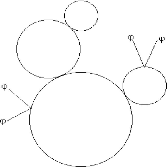
Figure 1: Generic 2PPR diagram

Let us consider a generic 2PPR diagram (two particle point reducible), i.e. a diagram that becomes disconnected when two internal lines meeting at the same point are cut (see fig. 1). It is clear that the 2PPR insertions are seagull (2 external $\phi$ lines) or bubble graphs. From that, we can conclude that the 2PPI expansion sums seagull and bubble graphs. How is this summation carried out ? We first notice that the seagull and bubble graphs contribute to the selfenergy as effective masses $\frac{\lambda}{2}\langle\phi\rangle^{2}$ and $\frac{\lambda}{2}\langle\phi^{2}\rangle_{c}=\frac{\lambda}{2}\Delta$ respectively. Therefore, one could naively think that all 2PPR insertions are summed by simply deleting the 2PPR graphs from the 1PI expansion and introducing the effective mass,

$$\overline{m}^{2}=m^{2}+\frac{\lambda}{2}(\varphi^{2}+\Delta)$$ (1)

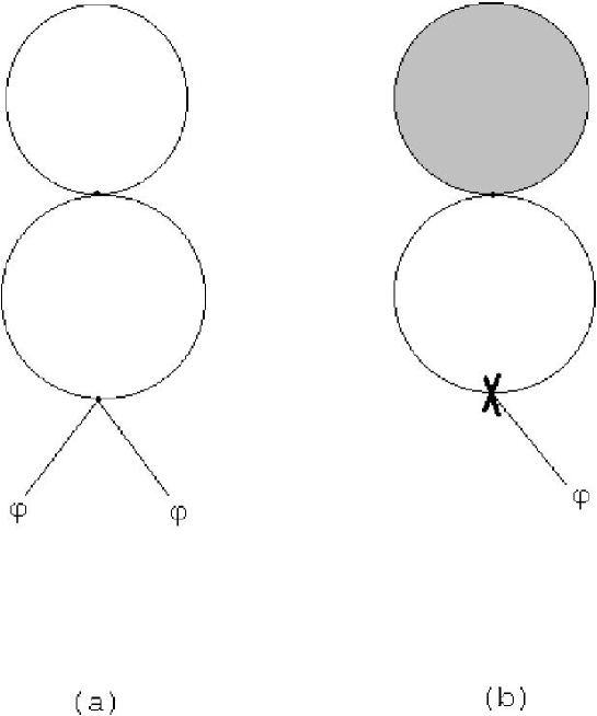
Figure 2: 2PPR part is shaded, 2PPI rest is earmarked

where $\varphi=\langle\phi\rangle$, in the remaining 2PPI graphs. This is not correct since there is a double counting problem which can be easily understood in the simple case of the 2loop vacuum graph (daisy graph with two petals) of fig. 2.a. Each petal can be seen as a self energy insertion in the other, so there is no way of distinguishing one or the other as the remaining 2PPI part. We could however earmark one of the petals by applying a derivative with respect to $\varphi$ (fig. 2.b). This way the 2PPI remainder (which contains the earmark) is uniquely fixed. Now, there are two ways in which the derivative can hit a $\varphi$ field. It can hit an explicit $\varphi$ field which is not a wing of a seagull or it can hit a wing of a seagull, i.e. an implicit $\varphi$ field hidden in the effective mass. We therefore have

$$\frac{\delta}{\delta\varphi}\Gamma^{1PI}_{q}(m^{2},\varphi)=\frac{\partial}{\partial\varphi}\Gamma^{2PPI}_{q}(\overline{m}^{2},\varphi)+\lambda\varphi\frac{\partial}{\partial\overline{m}^{2}}\Gamma^{2PPI}_{q}(\overline{m}^{2},\varphi)$$ (2)

where $\Gamma^{1PI}=S(\varphi)+\Gamma^{1PI}_{q}$. Using the definition (1) of the effective mass, we can rewrite this as :

$$\frac{\delta}{\delta\varphi}\Gamma^{1PI}_{q}(m^{2},\varphi)=\frac{\delta}{\delta\varphi}\Gamma^{2PPI}_{q}(\overline{m}^{2},\varphi)-\frac{\lambda}{2}\frac{\delta\Delta}{\delta\varphi}\frac{\partial\Gamma^{2PPI}_{q}}{\partial\overline{m}^{2}}(\overline{m}^{2},\varphi)$$ (3)

Using an analogous combinatorial argument we have

$$\frac{\partial\Gamma^{1}_{q}}{\partial m^{2}}(m^{2},\varphi)=\frac{\partial\Gamma^{2PPI}_{q}}{\partial\overline{m}^{2}}(\overline{m}^{2},\varphi)$$ (4)

and since $\Delta/2=\frac{\partial\Gamma^{1PI}_{q}}{\partial m^{2}}$, we find the following gap equation for $\Delta$ :

$$\frac{\Delta}{2}=\frac{\partial\Gamma^{2PPI}_{q}}{\partial\overline{m}^{2}}(\overline{m}^{2},\varphi)$$ (5)

The gap equation (5) can be used to integrate (3) and we finally obtain :

$$\Gamma^{1PI}(m^{2},\varphi)=S(\varphi)+\Gamma^{2PPI}_{q}(\overline{m}^{2},\varphi)-\frac{\lambda}{8}\int d^{D}x\Delta^{2}$$ (6)

with $\overline{m}^{2}$ the effective mass given by (1). So indeed, the 2PPR insertions can be summed into the effective mass $\overline{m}^{2}$ but there is a corection term (the last term in (6)) which accounts for double counting. This effective mass can be determined self consistently from the gap equation (5) which can be rewritten as :

$$\overline{m}^{2}=m^{2}+\frac{\lambda}{2}\varphi^{2}+\lambda\frac{\partial\Gamma^{2PPI}_{q}}{\partial\overline{m}^{2}}(\overline{m}^{2},\varphi)$$ (7)

Up till now, we have remained silent about renormalization. For example, $\Delta$ is quadratically divergent and needs renormalization. The question is if after renormalization, the simple relation (6) and the gap equation (5) remain valid. Fortunately, this is so if one uses a mass independent renormalization scheme. In [2] we showed that using dimensional regularization (which eliminates quadratic divergences) and a mass independent renormalization scheme, $\Delta$ can be renormalized as :

$$\Delta_{R}=Z_{2}\Delta+\delta Z_{2}\varphi^{2}+\frac{2\delta Z^{2PPR}_{2}}{\lambda}m^{2}$$ (8)

where renormalization constants come from the standard counterterm Lagrangian for $\lambda\phi^{4}$ :

$$\delta{\cal L}=\frac{\delta Z}{2}(\partial_{\mu}\phi)^{2}+\frac{\delta Z_{2}}{2}m^{2}\phi^{2}+\delta Z_{\lambda}\frac{\lambda\phi^{4}}{4!}$$ (9)

and $\delta Z^{2PPR}_{2}$ contains only the divergences from mass renormalization diagrams which are 2PPR. Using (8), one shows that the gap equation (5) becomes after renormalization :

$$\frac{\Delta_{R}}{2}=\frac{\partial\Gamma^{2PPI}_{q,R}}{\partial\overline{m}^{2}_{R}}(\overline{m}^{2}_{R},\varphi)$$ (10)

with $\overline{m}^{2}_{R}=m^{2}+\frac{\lambda}{2}(\varphi^{2}+\Delta_{R})$ and the relation (6) between $\Gamma^{1PI}$ and $\Gamma^{2PPI}_{q}$ becomes

$$\Gamma^{1PI}_{R}(\varphi,m^{2})=S(\varphi)+\Gamma^{2PPI}_{q,R}(\overline{m}^{2}_{R},\varphi)-\frac{\lambda}{8}\int d^{D}x\Delta^{2}_{R}$$ (11)

The 2PPI effective action is renormalized solely with 2PPI counterterms. The other 2PPR counterterms go into the renormalization of the effective mass $\overline{m}^{2}$. In minimal subtraction, equation (8) is automatically fulfilled and renormalization of the 2PPI expansion becomes extremely simple.

3 Effective potential at two loop 2PPI

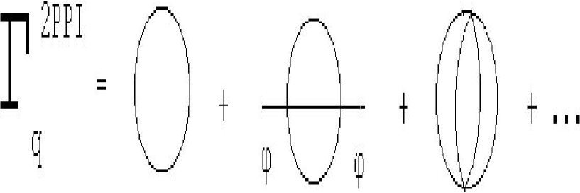
Figure 3: First terms of 2PPI expansion

From now on, we will work with the renormalized 2PPI expansion and drop the subscript R, keeping in mind that modified minimal subtraction ($\overline{MS}$ scheme) is implicity understood. The first few diagrams in het 2PPI expansion are displayed in figure 3. We use the imaginary time formalism and the Saclay method [8] to calculate the Matsubara sums. For the one loop contribution to the 2PPI effective potential, we find :

$$V^{2PPI}_{q}(\overline{m}^{2},\varphi) = \frac{1}{2}\sum\int\ln(k^{2}+\overline{m}^{2})$$ (12)

$$= \frac{\overline{m}^{4}}{64\pi^{2}}\left(\ln\frac{\overline{m}^{2}}{\overline{\mu}^{2}}-\frac{3}{2}\right)+Q_{T}(\overline{m}^{2})$$

where $\sum\int=T\begin{array}[t]{c}\sum\\[-5.0pt] \stackrel{{\scriptstyle n}}{{}}\end{array}\int\frac{d^{3}k}{(2\pi)^{3}},\overline{\mu}^{2}=4\pi e^{-\gamma}\mu^{2}$ and

$$Q_{T}(\overline{m}^{2})=T\int\frac{d^{3}q}{(2\pi)^{3}}\ln\left(1-e^{-\frac{E_{q}}{T}}\right)$$ (13)

The effective potential at one loop 2PPI (sum of daisy and superdaisy diagrams) is then given by :

$$V_{eff}(m^{2},\varphi,T)=\frac{m^{2}}{2}\varphi^{2}+\frac{\lambda}{4!}\varphi^{4}+\frac{\overline{m}^{4}}{64\pi^{2}}\left(\ln\frac{\overline{m}^{2}}{\overline{\mu}^{2}}-\frac{3}{2}\right)+Q_{T}(\overline{m}^{2})-\frac{\lambda}{8}\Delta^{2}$$ (14)

where $\overline{m}^{2}=m^{2}+\frac{\lambda}{2}(\varphi^{2}+\Delta)$ is a solution of the one loop gap equation

$$\overline{m}^{2}=m^{2}+\frac{\lambda\varphi^{2}}{2}+\frac{\lambda}{2}\left[\frac{\overline{m}^{2}}{16\pi^{2}}\left(\ln\frac{\overline{m}^{2}}{\overline{\mu}^{2}}-1\right)+P_{T}(\overline{m}^{2})\right]$$ (15)

with

$$P_{T}(\overline{m}^{2})=2\frac{\partial}{\partial\overline{m}^{2}}Q_{T}(\overline{m}^{2})=\int\frac{d^{3}q}{(2\pi)^{3}}\frac{n_{B}(q)}{E_{q}}$$ (16)

At two loops, the only 2PPI diagram we have to consider is the setting sun diagram. It has been calculated together with the other 2PPR two loop diagrams in [9]. For details, we refer to the appendix, especially with respect to 2PPI renormalization. For the effective potential at two loop 2PPI, we obtain the following expression :

$$V_{eff}(m^{2},\varphi,T) = \frac{m^{2}}{2}\varphi^{2}+\frac{\lambda}{4!}\varphi^{4}+\frac{\overline{m}^{4}}{64\pi^{2}}\left(\ln\frac{\overline{m}^{2}}{\overline{\mu}^{2}}-\frac{3}{2}\right)+Q_{T}(m^{2})$$ (17)

$$- \frac{\lambda}{8}\Delta^{2}-\frac{\lambda^{2}}{12}\varphi^{2}(G_{0}(\overline{m}^{2})+G_{1}(\overline{m}^{2},T)+G_{2}(\overline{m}^{2},T))$$

where

$$G_{0}(\overline{m}^{2})=-\frac{3}{2}\frac{\overline{m}^{2}}{(4\pi)^{4}}\left(\ln^{2}\frac{\overline{\mu}^{2}}{\overline{m}^{2}}+4\ln\frac{\overline{\mu}^{2}}{\overline{m}^{2}}+4+\frac{\pi^{2}}{6}-\frac{8.966523919}{3}\right)$$ (18)

$$G_{1}(\overline{m}^{2},T) = \frac{3}{(4\pi)^{2}}\left(\ln\frac{\overline{\mu}^{2}}{\overline{m}^{2}}+2\right)\int\frac{d^{3}q_{1}}{(2\pi)^{3}}\frac{n_{B}(q_{1})}{E_{q_{1}}}$$ (19)

$$+ \frac{3}{4(2\pi)^{4}}\int^{\infty}_{0}dq_{1}\frac{q_{1}n_{B}(q_{1})}{E_{q_{1}}}\int^{\infty}_{0}\frac{dq_{2}}{E_{q_{2}}}\left(q_{2}\ln|\frac{X_{+}}{X_{-}}|-4q_{1}\right)$$

with

$$X_{\pm}=\left(E_{q_{1}}+E_{q_{2}}+E_{q_{1}\pm q_{2}}\right)^{2}\times\left(-E_{q_{1}}+E_{q_{2}}+E_{q_{1}\pm E_{2}}\right)^{2}$$ (20)

$$G_{2}(\overline{m}^{2},T)=\frac{3}{4(2\pi)^{4}}\int^{\infty}_{0}dq_{1}\frac{q_{1}n_{B}(q_{1})}{E_{q_{1}}}\int^{\infty}_{0}dq_{2}\frac{q_{2}n_{B}(q_{2})}{E_{q_{2}}}\ln|\frac{Y_{+}}{Y_{-}}|$$ (21)

with

$$Y_{\pm} = (E_{q_{1}}+E_{q_{2}}+E_{q_{1}\pm q_{2}})^{2}\times(-E_{q_{1}}+E_{q_{2}}+E_{q_{1}\pm q_{2}})^{2}$$ (22)

$$\times (E_{q_{1}}-E_{q_{2}}+E_{q_{1}\pm q_{2}})^{2}\times(E_{q_{1}}+E_{q_{2}}-E_{q_{1}\pm q_{2}})^{2}$$

The effective mass $\overline{m}^{2}$ is a solution of the 2 loop gap equation :

$$\overline{m}^{2} = m^{2}+\frac{\lambda\varphi^{2}}{2}+\frac{\lambda}{2}\left[\frac{\overline{m}^{2}}{16\pi^{2}}\left(\ln\frac{\overline{m}^{2}}{\overline{\mu}^{2}}-1\right)+P_{T}(\overline{m}^{2})\right.$$ (23)

$$- \frac{\lambda^{2}\varphi^{2}}{6}\left.\left(\frac{\partial G_{0}(\overline{m}^{2})}{\partial\overline{m}^{2}}+\frac{\partial G_{1}(\overline{m}^{2},T)}{\partial\overline{m}^{2}}+\frac{\partial G_{2}(\overline{m}^{2},T)}{\partial\overline{m}^{2}}\right)\right]$$

4 Numerical results

The results obtained in the previous section were used to calculate the effective potential for $\lambda\phi^{4}$-theory at the 2-loop 2PPI level numerically. These calculations involved two steps. The first one is the numerical integration of the double integrals in ( 19) and ( 21). Both integrals should be integrated from $0$ tot $\infty$. However we found that is was sufficient to approximate the infinite integration interval by the compact interval $[0,10^{5}]$. The stability of the numerical results towards changes in this interval and changes in the parameters of the model was checked and found to be satisfactory. A second difficulty arises from the need to solve the gap equation which is a transcendental equation. Trying to calculate the effective 2PPI potential as a function of $\varphi$, we need to solve the gap equation ( 23) which gives us the variational mass $\overline{m}$ as a function of $\varphi$. This could be done by iteration, but this approach will demand a lot of computational ressources. We opted for a different approach, which consists of determining $\varphi$ as a function of the mass, calculate $V(\varphi(\overline{m}^{2}),\overline{m}^{2})$ and plot $V(\varphi)$ by varying $\overline{m}$.

The parameters in our Lagrangian and the renormalization scale $\overline{\mu}$ were chosen in such a way that comparison with the work of Chiku [13], which also uses an effective mass to improve upon the 1PI loop expansion, would be easy. We refer to this paper for more details about this choice of parameters. We used the two parameter sets used by Chiku in [13] and found that the results did not depend qualitatively on the particular set. The numerical results in this section have been obtained with $\lambda=10.0,m^{2}=-170$ and $\overline{\mu}^{2}=87.6$.

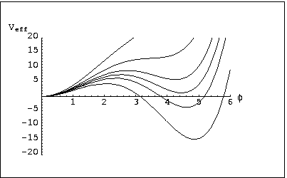
Figure 4: The 1-loop effective potential at T=21.5,21.6,21.65,21.7,21.8,22. At 1-loop we see a clear first order transition.

In figure 4 the 1-loop 2PPI effective potential $V(\varphi)$ is shown for temperatures in the neighbourhood of the critical temperature. This figure clearly indicates a first order transition. Attention should be payed to the fact that this first order transition may easily be mistaken for a second order one if looked at at a larger scale. Therefore, it is necessary to use a sufficiently fine grid of points around $\varphi_{0}$ where the potential reaches its minimum, and to look at temperatures which are sufficiently close to the critical temperature. The transition also manifests itself as a discontinuity in the evolution of $\varphi_{0}$ at the critical temperature where $\varphi_{0}$ jumps from about 0.4 to 0. (figure 5).

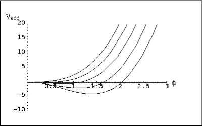
Figure 6: The 2-loop effective potential at T = 23.8,24,24.2,24.4,24.6 . Including the SS-diagram changes the 1-loop first order transition to a second order one.

Including the setting sun diagram, the 2PPI effective potential is altered to exhibit a second order phase transition, as can be seen from figure 6. The second order nature of this transition was extensively checked in the neighbourhood of the critical temperature $T_{c}=24.421$. It is also evident from the continuous descent of $\varphi_{0}$ towards zero, where the symmetry is restored (figure 7). In figure 7 there seems to be a shoulder structure for which we have no physical explanation.

All of the above mentioned results show qualitative agreement with the 2-loop analysis of $\lambda\phi^{4}$ theory in optimised perturbation theory, as done by Chiku in [13]

For the critical exponent $\beta$, which is defined by

$$\varphi_{0}(T)\sim\left|\frac{T-T_{c}}{T_{c}}\right|^{\beta}$$

for temperatures close to the critical temperature, we found the value $\beta=0.52$ when taking the temperature interval $[24,24.421]$, indicating consistency with the Landau mean-field theory which predicts $\beta=0.5$. As a check for this last claim, we also investigated the critical behaviour of the second derivative of the effective potential and found again accordance with the Landau mean-field prediction.

Summarizing, in this paper we have analysed the $\lambda\phi^{4}$ theory at finite temperature using the 2PPI expansion at the 2 loop order. We found that the inclusion of the setting sun diagram which is the only two loop 2PPI diagram, changes the phase transition from first order at one loop 2PPI to second order at two loop 2PPI. The critical exponents we found were mean field. We do not believe that adding more terms of the 2PPI expansion will improve the critical exponents. We expect that renormalization group resummation of the 2PPI expansion [14] is necessary to breng the critical exponents in closer agreement with experiment.

Appendix

In this appendix, we will calculate and renormalize the setting sun diagram. Because this is a 2PPI diagram, only the 2PPI counterterms have to be taken into account. The 2PPR counterterms are used to renormalize 2PPR insertions in 2PPI diagrams. This is a different approach than ordinary 1PI renormalization where all the 2loop diagrams (two bubble and setting sun graphs) have to be considered together and all one loop counterterms have to be inserted [10]. In [2] we showed that both approaches are equivalent and the purpose of this appendix is mainly to check this explicitely at two loops. For those aspects of the calculations which are not related to renormalization, we will borrow heavily from [9] to which we refer for further details.

Using the Saclay method, we find the following expression for the setting sun diagram :

$$I_{ss}=\frac{\lambda^{2}}{6}[G_{0}(\overline{m}^{2})+G_{1}(\overline{m}^{2},T)+G_{2}(\overline{m}^{2},T)]$$ (1)

where $G_{0}$ is the temperature independent part

$$G_{0}(\overline{m}^{2}) = \int\frac{d^{D}q_{1}}{(2\pi)^{D}}\int\frac{d^{D}q_{1}}{(2\pi)^{D}}\frac{1}{q^{2}_{1}+\overline{m}^{2}}\frac{1}{q^{2}_{2}+\overline{m}^{2}}\frac{1}{(q_{1}+q_{2})^{2}+\overline{m}^{2}}$$ (2)

$$= 3\int d[q_{1},q_{2}]S(E_{q_{1}},E_{q_{2}},E_{q_{3}})$$

with

$$d[q_{1},q_{2}]=\frac{d^{D-1}q_{1}}{(2\pi)^{D-1}}\frac{d^{D-1}q_{2}}{(2\pi)^{D-1}}\frac{1}{8E_{q_{1}}E_{q_{2}}E_{q_{3}}}$$ (3)

$$S(E_{q_{1}},E_{q_{2}},E_{q_{3}})=\frac{2}{E_{q_{1}}+E_{q_{2}}+E_{q_{3}}}$$ (4)

and $q_{3}=-(q_{1}+q_{2})$ and where $G_{1}$ and $G_{2}$ are temperature dependent with one and two Bose-Einstein factors respectively :

$$G_{1}(\overline{m}^{2},T)=3\int d[q_{1},q_{2}]n_{B}(q_{1})\left[S(E_{q_{1}},E_{q_{2}}E_{q_{3}})+S(-E_{q_{1}},E_{q_{2}},E_{q_{3}})\right]$$ (5)

$$G_{2}(\overline{m}^{2},T) = 3\int d[q_{1},q_{2}]n_{B}(q_{1})n_{B}(q_{2})\left[S(E_{q_{1}},E_{q_{2}},E_{q_{3}})+S(-E_{q_{1}},E_{q_{2}},E_{q_{3}})\right.$$ (6)

$$+ \left.S(E_{q_{1}},-E_{q_{2}},E_{q_{3}})-S(E_{q_{1}},E_{q_{2}},-E_{q_{3}})\right]$$

The setting sun diagram at T = 0 has been calculated in [11,12] in $D=4-2\epsilon$ :

$$G_{0}(\overline{m}^{2})=\mu^{4\epsilon}\frac{(\overline{m}^{2})^{1-2\epsilon}}{(4\pi)^{4-2\epsilon}}\Gamma(2\epsilon-1)\left(\frac{3}{\epsilon}+3-8.966523919\epsilon+...\right)$$ (7)

Doing the integral over the angle between $q_{1}$ and $q_{2}$, $G_{1}(\overline{m}^{2},T)$ can be separated in divergent and finite parts [9] :

$$G_{1}(\overline{m}^{2},T) = \frac{3}{(4\pi)^{2}}I^{\epsilon}_{\beta}(\overline{m}^{2})\frac{1}{\epsilon}+\frac{3}{(4\pi)^{2}}I^{0}_{\beta}(\overline{m}^{2})\left[2+\ln\frac{\overline{\mu}^{2}}{\overline{m}^{2}}\right]$$ (8)

$$+ \frac{3}{4(2\pi)^{4}}\int^{\infty}_{0}dq_{1}\frac{q_{1}n_{B}(q_{1})}{E_{q_{1}}}\int^{\infty}_{0}\frac{dq_{2}}{E_{q_{2}}}\left[q_{2}\ln|\frac{X_{+}}{X_{-}}|-4q_{1}\right]$$

with

$$X_{\pm}=(E_{q_{1}}+E_{q_{2}}+E_{q_{1}\pm q_{2}})^{2}\times(-E_{q_{1}}+E_{q_{2}}+E_{q_{1}\pm q_{2}})^{2}$$ (9)

and

$$I^{\epsilon}_{\beta}(\overline{m}^{2})=\mu^{4\epsilon}\int\frac{dq^{3-2\epsilon}}{(2\pi)^{3-2\epsilon}}\frac{n_{B}(q)}{E_{q}}$$ (10)

Because $G_{2}$ has a Bose-Einstein factor for each momentumvariable, it is U.V. finite and after doing the angular integration one finds :

$$G_{2}(\overline{m}^{2},T)=\frac{3}{4(2\pi)^{4}}\int^{\infty}_{0}dq_{1}\frac{q_{1}n_{B}(q_{1})}{E_{q_{1}}}\int^{\infty}_{0}dq_{2}\frac{q_{2}n_{B}(q_{2})}{E_{q_{2}}}\ln|\frac{Y_{+}}{Y_{-}}|$$ (11)

with

$$Y_{\pm} = \left(E_{q_{1}}+E_{q_{2}}+E_{q_{1}\pm q_{2}}\right)^{2}\times\left(-E_{q_{1}}+E_{q_{2}}+E_{q_{1}\pm q_{2}}\right)^{2}$$ (12)

$$\times \left(E_{q_{1}}-E_{q_{2}}+E_{q_{1}\pm q_{2}}\right)^{2}\times\left(E_{q_{1}}+E_{q_{2}}-E_{q_{1}\pm q_{2}}\right)^{2}$$

We now investigate the renormalization of the setting sun diagram at finite temperature in some more detail. Since the counterterm Lagrangian is

$$\delta{\cal L}=\frac{1}{2}\delta Z(\partial_{\mu}\phi)^{2}+\frac{1}{2}\delta Z_{2}m^{2}\phi^{2}+\frac{1}{4!}\delta Z_{4}\lambda\phi^{4}$$ (13)

we find from

$$\parbox{20.0pt}{\begin{picture}(50.0,20.0)\GCirc(10,10){5}{1} \Line(1,5)(5,10) \Line(1,15)(5,10) \Line(15,10)(19,15) \Line(15,10)(19,5)\end{picture}}+\mbox{crossing}+\parbox{20.0pt}{\begin{picture}(20.0,20.0)\Line(3,3)(10,10) \Line(17,3)(10,10)\Line(17,17)(10,10)\Line(3,17)(10,10)\Text(10,10)[c] {$\otimes$} \end{picture}} =$$ finite

$$\parbox{20.0pt}{\begin{picture}(20.0,20.0)\Oval(10,15)(5,4)(0) \Line(0,10)(20,10) \end{picture}}+\parbox{20.0pt}{\begin{picture}(20.0,20.0)\Line(0,10)(6.5,10) \Text(10,10)[c]{$\otimes$} \Line(13.5,10)(20,10) \end{picture}} =$$ finite (14)

that at one loop

$$\delta Z=0,\delta Z_{2}=\frac{1}{32\pi^{2}}\lambda\frac{1}{\epsilon},\delta Z_{4}=\frac{3}{32\pi^{2}}\lambda\frac{1}{\epsilon}$$ (15)

In [2] it was shown that

$$\delta Z^{2PPR}_{4}=\delta Z_{2}$$ (16)

so that

$$\delta Z^{2PPI}_{4}=\delta Z_{4}-\delta Z_{2}=\frac{1}{16\pi^{2}}\lambda\frac{1}{\epsilon}$$ (17)

To renormalize the setting sun diagram which is 2PPI, we only have to include 2PPI counterterms

$$\parbox{20.0pt}{\begin{picture}(20.0,20.0)\GCirc(10,10){7}{1} \Line(0,10)(20,10)\end{picture}}+\parbox{20.0pt}{\begin{picture}(20.0,20.0)\Oval(10,15)(5,4)(0) \Line(0,10)(6.5,10) \Text(10,10)[c]{$\otimes$} \Line(13.5,10)(20,10) \Text(10,2)[c]{\tiny{2PPI}} \end{picture}}+\parbox{20.0pt}{\begin{picture}(20.0,20.0)\Line(0,10)(6.5,10) \Text(10,10)[c]{$\otimes$} \Line(13.5,10)(20,10) \Text(10,2)[c]{\tiny{2PPI}} \end{picture}}=\mbox{finite}$$ (18)

This equation determines the two loop 2PPI part of mass renormalization. When using the 2PPI counterterm for mass renormalisation of 2PPI diagrams, we should keep in mind to replace the ordinary mass $m^{2}$ with the effective mass $\overline{m}^{2}$. This is correct to all orders as was shown in [2]. Coupling constant renormalization gives :

(19)

$$= -\frac{1}{2}\frac{\lambda^{2}}{(4\pi)^{2}}\frac{1}{\epsilon}\left(I_{0}(\overline{m}^{2})+I^{\epsilon}_{\beta}(\overline{m}^{2})\right)$$

with

$$I_{0}(\overline{m}^{2}) = \frac{\overline{m}^{2}}{(4\pi)^{2}}\left(\frac{4\pi\mu^{2}}{\overline{m}^{2}}\right)^{\epsilon}\Gamma(\epsilon-1)$$ (20)

$$= \frac{\overline{m}^{2}}{(4\pi)^{2}}\left[-\frac{1}{\epsilon}+\ln\frac{\overline{m}^{2}}{\overline{\mu}^{2}}-1+0(\epsilon)\right]$$

From (A.1) and (A.7), we have

$$\parbox{20.0pt}{\begin{picture}(20.0,20.0)\GCirc(10,10){7}{1} \Line(0,10)(20,10) \Text(10,0)[c]{\tiny{$T=0$}} \end{picture}}=-\frac{\lambda^{2}}{4}\frac{\overline{m}^{2}}{(4\pi)^{4}}\left[\frac{1}{\epsilon^{2}}+\frac{3}{\epsilon}-\frac{2}{\epsilon}\ln\left(\frac{\overline{m}^{2}}{\overline{\mu}^{2}}\right)\right]+\mbox{finite}$$ (21)

As a check on 2PPI renormalization, we find that the $\frac{1}{\epsilon}\ln\overline{m}^{2}/\overline{\mu}^{2}$ term coming from overlapping divergences gets nicely cancelled and that at two loops

$$\delta Z^{2PPI}_{2}=\frac{\lambda^{2}}{4}\frac{1}{(4\pi)^{4}}\left(\frac{1}{\epsilon^{2}}-\frac{1}{\epsilon}\right)$$ (22)

Analogously, we find from (A.1), (A.8) and (A.19) that the temperature dependent divergent part gets exactly cancelled by the 2PPI counterterm diagram. Doing the renormalization to $0(\epsilon^{0})$, one finds that the finite parts of $G_{0}$, $G_{1}$ and $G_{2}$ are given respectively by (18), (19) and (21) of section 3.

Figure 5: The 1-loop calculation of $\phi_{0}$ where the potential reaches it’s minimum at different temperatures shows a discontinuous jump to zero at the critical temperature.

Figure 7: The 2-loop calculation of $\phi_{0}$ shows a continuous approach to zero at the critical temperature.

References

- [1] H. Verschelde and M. Coppens, Phys. Lett. B287 (1992) 133
- [2] H. Verschelde, Phys. Lett. B497 (2001)165
- [3] J.M. Cornwall, R. Jackiw and E. Tomboulis, Phys. Rev. D10 (1974) 2428
- [4] H. Verschelde and J. De Pessemier, hep-th/0009241
- [5] L. Dolan and R. Jackiw, Phys. Rev. D9 (1974) 3357
- [6] G. Amelino-Camelia and So-Young Pi, Phys. Rev. D47 (1993) 2356
- [7] C.G. Boyd, D.E. Brahmand S.D.H. Hsu, Phys. Rev. D48 (1993) 4963
- [8] R.D. Pisarski, Nucl. Phys. B309 (1988) 476
- [9] R.R. Parwani, Phys. Rev. D45 (1992) 4695; erratum, D48 (1993) 5965
- [10] P. Ramond, Field Theory: A Modern Primer (Addison-Wesley,1990)
- [11] A.I. Davydychev and J.B. Tausk, Nucl. Phys.B397 (1993) 123
- [12] K. Knecht and H. Verschelde, hep-th/9712449
- [13] S. Chiku, Prog. Theor. Phys. 104 (2000) 1129
- [14] H. Verschelde and M. Coppens, Phys. Lett. B295 (1992) 8