Six-dimensional Abelian vortices
with quadratic curvature self-interactions

Abstract

Six-dimensional Nielsen-Olesen vortices are analyzed in the context of a quadratic gravity theory containing Euler-Gauss-Bonnet self-interactions. The relations among the string tensions can be tuned in such a way that the obtained solutions lead to warped compactification on the vortex. New regular solutions are possible in comparison with the case where the gravity action only consists of the Einstein-Hilbert term. The parameter space of the model is discussed.

Preprint Number: UNIL-IPT-01-12, August 2001

I Introduction

Higher dimensional gravity theories have been discussed in connection with possible alternatives to Kaluza-Klein compactification [1, 2, 3, 4, 5, 6]. In this context the gravity part of the action usually consists of the Einstein-Hilbert term possibly supplemented by a bulk cosmological constant.

If extra-dimensions are not compact, it is interesting to relax the assumption that gravity is described purely in terms of the Einstein-Hilbert action. Indeed, various investigations took into account the possible contribution of higher derivatives terms in the bulk action and mainly in the case of one bulk coordinate [7, 8, 9, 10, 11]. The motivations of these studies range from the possible connection to string motivated scenarios [7] to the possibility of obtaining warped compactifications in quadratic gravity theories [12, 13] defined in more than four dimensions. Quadratic corrections may also play a rôle in the context of AdS/CFT correspondence [14].

Recently, it has been shown that gravity can be localized on a Nielsen-Olesen vortex in the context of the Abelian-Higgs model [15] in a six dimensional space-time. This explicit model leads to warped compactification and it represents an explicit field theoretical realization of the suggestion that a string in six dimensions can lead to the localization of gravity [16] provided certain relations among the string tensions are satisfied. In the investigations dealing with higher dimensional topological defects (like strings [17, 18, 19, 20, 21], monopoles [22, 23, 24], or instantons [25, 26, 27]) the space time metric is defined in more than five dimensions, but, still, the gravity part of the action is assumed to be the Einstein-Hilbert term possibly supplemented by a bulk cosmological constant .

We would like to understand if it is possible to obtain warped solutions in the context of the gravitating Abelian-Higgs model in six dimensions when quadratic curvature corrections are present. The brane action will be the one provided by the Abelian-Higgs model [31] generalized to the case of six (gravitating) dimensions. The quadratic corrections to the Einstein-Hilbert action will be taken in the Euler-Gauss-Bonnet (EGB) form. This choice has the interesting property of preserving the relations among the string tensions derived in the case when the gravity action is in the Einstein-Hilbert form.

Previous studies suggest that if the Einstein Hilbert action is supplemented by quadratic curvature corrections, geometries leading to warped compactification in more than five dimensions can be obtained. More specifically, in [32] seven-dimensional warped solutions have been discussed in the case when hedgehogs configurations are present together with quadratic self-interactions parametrized in the Euler-Gauss-Bonnet form. In [33] the simultaneous presence of dilaton field and quadratic corrections has been investigated in a string theoretical perspective and mainly in six-dimensions.

The plan of this paper is the following. In Section II the main equations of the system are derived. Section III is devoted to the analysis of the asymptotics of the solutions in the presence of EGB corrections. Section IV contains the study of the relations among the string tensions, whereas Section V deals with the analysis of the various classes of solutions which can be found in the presence of quadratic corrections. In Section VI the analysis of the parameter space of the model is presented. Section VII contains our concluding remarks.

II Brane sources with quadratic gravity in the bulk

In more than four dimensions the Einstein-Hilbert term is not the only geometrical action leading to equations of motion involving second order derivatives of the metric [12]. The usual Einstein-Hilbert invariant can indeed be supplemented with higher order curvature corrections without generating, in the equations of motion, terms containing more than two derivatives of the metric with respect to the space-time coordinates [13]. If this is the case, the quadratic part of the action can be written in terms of the Euler-Gauss-Bonnet combination:

$${\cal R}^{2}_{\rm EGB}=R^{ABCD}R_{ABCD}-4R^{AB}R_{AB}+R^{2}.$$ (2.1)

In four dimensions the EGB is a topological term and it coincides with the Euler invariant: its contribution to the equations of motion can be rearranged in a perfect four-divergence which does not contribute to the classical equations of motion. In more than four dimensions the EGB combination leads to a ghost-free theory and it appears in different higher dimensional contexts. In string theory the (tree-level) low energy effective action is supplemented not only by an expansion in the powers of the dilaton coupling but also by an expansion in powers of the string tension $\alpha^{\prime}$. The EGB indeed appears in the first $\alpha^{\prime}$ correction [35, 36, 37, 38]. In supergravity the EGB is required in order to supersymmetrize the Lorentz-Chern-Simons term.

The brane source will be described in terms of the Abelian-Higgs model [31] appropriately generalized to the six-dimensional case [15]:

$$S_{\rm brane}=\int d^{6}x\sqrt{-G}\biggl{[}\frac{1}{2}({\cal D}_{A}\phi)^{*}{\cal D}^{A}\phi-\frac{1}{4}F_{AB}F^{AB}-\frac{\lambda}{4}\left(\phi^{*}\phi-v^{2}\right)^{2}\biggr{]}~{},$$ (2.2)

where ${\cal D}_{A}=\nabla_{A}-ieA_{A}$ is the gauge covariant derivative, while $\nabla_{A}$ is the generally covariant derivative .

The bulk action will then be taken in the form

$$S_{\rm bulk}=-\int d^{6}x\sqrt{-G}\biggl{[}\frac{R}{2\chi}+\Lambda-\alpha^{\prime}{\cal R}^{2}_{\rm EGB}\biggr{]}.$$ (2.3)

This gravitational effective action can be related to the low energy string effective action (corrected to first order in the string tension) provided the dilaton and antisymmetric tensor field are frozen to a constant value [36]. Since $\chi=8\pi G_{6}=8\pi/M_{6}^{4}$, we have that, dimensionally, $\alpha^{\prime}=[M_{6}]^{2}$.

With these conventions, the equations of motion of the system can be obtained and they are:

$$G^{AB}\nabla_{A}\nabla_{B}\phi-e^{2}A_{A}A^{A}\phi-ieA_{A}\partial^{A}\phi-ie\nabla_{A}(A^{A}\phi)+\lambda(\phi^{*}\phi-v^{2})\phi=0,$$ (2.4)

$$\nabla_{A}F^{AB}=-e^{2}A^{B}\phi^{*}\phi+\frac{ie}{2}\left(\phi\partial^{B}\phi^{*}-\phi^{*}\partial^{B}\phi\right),$$ (2.5)

$$R_{AB}-\frac{1}{2}G_{AB}R=\chi\left(T_{AB}+\Lambda G_{AB}\right)-2\alpha^{\prime}\chi{\cal Q}_{AB},$$ (2.6)

where

$$T_{AB} = \biggl{[}\frac{1}{2}({\cal D}_{M}\phi)^{*}{\cal D}^{M}\phi-\frac{1}{4}F_{MN}F^{MN}-\frac{\lambda}{4}\left(\phi^{*}\phi-v^{2}\right)^{2}\biggr{]}G_{AB}\,$$ (2.7)

$$+ \,\frac{1}{2}\left[({\cal D}_{A}\phi)^{*}{\cal D}_{B}\phi+({\cal D}_{B}\phi)^{*}{\cal D}_{A}\phi\right]-\,F_{AC}{F_{B}}^{C},$$ (2.8)

and where

$${\cal Q}_{AB}=\frac{1}{2}G_{AB}{\cal R}_{\rm EGB}^{2}-2RR_{AB}+4R_{AC}R^{~{}~{}C}_{B}+4R_{CD}R_{A~{}B}^{~{}~{}C~{}~{}D}-2R_{ACDE}R_{B}^{~{}~{}CDE}$$ (2.9)

is the Lanczos tensor appearing as a result of the EGB contribution in the action.

Defining as $n$ the winding number, the Nielsen-Olesen ansatz [31] can be generalized to six-dimensional space-time

$$\phi(\rho,\theta)=vf(\rho)e^{i\,n\,\theta},$$ (2.10)

$$A_{\theta}(\rho,\theta)=\frac{1}{e}[\,n\,-\,P(\rho)]~{},$$ (2.11)

where $\rho$ and $\theta$ are, respectively, the bulk radius and the bulk angle covering the transverse space of the metric

$$ds^{2}=G_{AB}dx^{A}dx^{B}=M^{2}(\rho)g_{\mu\nu}dx^{\mu}dx^{\nu}-d\rho^{2}-L(\rho)^{2}d\theta^{2}.$$ (2.12)

In Eq. (2.12), we will choose, for simplicity $g_{\mu\nu}\equiv\eta_{\mu\nu}$ where $\eta_{\mu\nu}$ is the Minkowski metric.

The equations of motion for the gauge-Higgs system can then be written. Using Eqs. (2.11)–(2.12) into Eqs. (2.4)–(2.6) the following system of equations is obtained:

$$f^{\prime\prime}+(4m+\ell)f^{\prime}+(1-f^{2})f-\frac{P^{2}}{{\cal L}^{2}}f=0,$$ (2.13)

$$P^{\prime\prime}+(4m-\ell)P^{\prime}-\alpha f^{2}P=0,$$ (2.14)

$$\ell^{\prime}+3m^{\prime}+\ell^{2}+6m^{2}+3lm=-\mu-\nu\tau_{0}+\epsilon{\cal G}_{0},$$ (2.15)

$$4m^{\prime}+10m^{2}=-\mu-\nu\tau_{\theta}+\epsilon{\cal G}_{\theta},$$ (2.16)

$$4m\ell+6m^{2}=-\mu-\nu\tau_{\rho}+\epsilon{\cal G}_{\rho}.$$ (2.17)

Eqs. (2.13) and (2.14) correspond, respectively, to the evolution equations for the Higgs field and for the gauge field. The remaining equations come from the various components of Eq. (2.6). In Eqs. (2.15)–(2.17) the non-vanishing components of the energy-momentum tensor are

$$\tau_{0}(x) \equiv T_{0}^{0}=T_{i}^{i}=\frac{{f^{\prime}}^{2}}{2}+\frac{1}{4}(f^{2}-1)^{2}+\frac{{P^{\prime}}^{2}}{2\alpha{\cal L}^{2}}+\frac{f^{2}P^{2}}{2{\cal L}^{2}},$$ (2.18)

$$\tau_{\rho}(x) \equiv T_{\rho}^{\rho}=-\frac{{f^{\prime}}^{2}}{2}+\frac{1}{4}(f^{2}-1)^{2}-\frac{{P^{\prime}}^{2}}{2\alpha{\cal L}^{2}}+\frac{f^{2}P^{2}}{2{\cal L}^{2}},$$ (2.19)

$$\tau_{\theta}(x) \equiv T_{\theta}^{\theta}=\frac{{f^{\prime}}^{2}}{2}+\frac{1}{4}(f^{2}-1)^{2}-\frac{{P^{\prime}}^{2}}{2\alpha{\cal L}^{2}}-\frac{f^{2}P^{2}}{2{\cal L}^{2}}.$$ (2.20)

Finally, the functions ${\cal G}$ appearing in Eqs. (2.15)–(2.17) are the non-vanishing components of the Lanczos tensor ${\cal Q}_{AB}$:

$${\cal G}_{0} = 36\ell m^{3}+12m^{4}+12m^{2}\ell^{\prime}+12m^{2}\ell^{2}++24\ell mm^{\prime}+12m^{2}m^{\prime},$$ (2.21)

$${\cal G}_{\rho} = 12m^{4}+48m^{3}\ell,$$ (2.22)

$${\cal G}_{\theta} = 48m^{2}m^{\prime}+60m^{4}.$$ (2.23)

Eqs. (2.13)–(2.17) are written in terms of the rescaled parameters:

$${\cal L}(x)=\frac{m_{H}}{\sqrt{2}}L(\rho),~{}~{}~{}\alpha=2\frac{m^{2}_{V}}{m^{2}_{H}},~{}~{}~{}\mu=\frac{2\chi\Lambda}{m^{2}_{H}},~{}~{}~{}\nu=\chi\frac{m^{2}_{H}}{2\lambda},$$ (2.24)

where $m_{H}=\sqrt{2\lambda}v$ is the Higgs mass and $m_{V}=e~{}v$ is the vector boson mass. In Eq. (2.13)–(2.17) the prime denotes the derivative with respect to $x=m_{H}\rho/\sqrt{2}$ (the rescaled bulk radius) and $m(x)=M^{\prime}/M$ , $\ell(x)={\cal L}^{\prime}/{\cal L}$. In Eqs. (2.13)–(2.17) the $\epsilon=\alpha^{\prime}\chi m_{H}^{2}$ has been defined. This parameter controls the higher derivative corrections.

III Asymptotics of the solutions

In order to discuss regular solutions describing a thick brane in six dimensions and in the presence of EGB self-interactions it is important to understand the asymptotic behaviour of the geometry and of the matter fields of the model. Quadratic curvature corrections affect the asymptotics of the geometry and the asymptotics of the scalar and gauge fields.

A Bulk solutions

Far from the core of the defect, the equations determining the bulk solutions are given by

$$m^{\prime}=-\frac{5}{2}m^{2}-\frac{\mu+60\epsilon m^{4}}{4(1-12\epsilon m^{2})},$$ (3.1)

$$\ell=-\frac{m}{4}-\frac{\mu+5m^{2}}{4m(1-12\epsilon m^{2})}.$$ (3.2)

From Eq. (3.1), $m(x)$ can be determined and Eq. (3.2) will then give $\ell(x)$. If $m^{\prime}(x)=0$ and $\ell^{\prime}(x)=0$ a consistent solution can be found provided $\ell(x)=m(x)$. In this case $m$ should satisfy the following quartic equation

$$60\epsilon m^{4}-10m^{2}-\mu=0.$$ (3.3)

whose solution can be written as

$$m^{2}=\frac{1}{12\epsilon}\biggl{(}1\pm\sqrt{1+\frac{12}{5}\epsilon\mu}\biggr{)}.$$ (3.4)

Defining now

$$\gamma_{1}=\frac{1}{12\epsilon}\biggl{(}1+\sqrt{1+\frac{12}{5}\epsilon\mu}\biggr{)},$$ (3.5)

$$\gamma_{2}=\frac{1}{12\epsilon}\biggl{(}1-\sqrt{1+\frac{12}{5}\epsilon\mu}\biggr{)},$$ (3.6)

warped solutions will correspond either to $m_{1}\sim-\sqrt{\gamma_{1}}$ or to $m_{2}\sim-\sqrt{\gamma_{2}}$. As a consequence, the behaviour of the metric functions will be either

$$M(x)\sim M_{0}e^{-\sqrt{\gamma_{1}}x},\,\,\,{\cal L}(x)\sim{\cal L}_{0}e^{-\sqrt{\gamma_{1}}x},$$ (3.7)

or

$$M(x)\sim M_{0}e^{-\sqrt{\gamma_{2}}x},\,\,\,{\cal L}(x)\sim{\cal L}_{0}e^{-\sqrt{\gamma_{2}}x}.$$ (3.8)

Since $\gamma_{1}$ and $\gamma_{2}$ must both be positive for warped solutions, not all the signs of $\epsilon$ and $\mu$ are compatible with the behaviour of Eqs. (3.7)–(3.8). More precisely, if $\epsilon>0$ and $\mu>0$ only the solution $\gamma_{1}$ is possible. If $\epsilon<0$ and $\mu<0$ only the solution $\gamma_{2}$ is possible. If $\epsilon>0$ and $\mu<0$ both, $\gamma_{1}$ and $\gamma_{2}$, lead to warped geometries. Finally, if $\mu>0$ and $\epsilon<0$ no solution is possible. The situation can be summarized in the following table.

	$\epsilon>0$	$\epsilon<0$
$\mu>0$	$\gamma_{1}$	$\emptyset$
$\mu<0$	$\gamma_{1},~{}\gamma_{2}$	$\gamma_{2}$

Let us now investigate what happens if $m(x)\neq\ell(x)$. Subtracting Eq. (2.17) from Eq. (2.16) we obtain

$$(1-12\epsilon m^{2})[m^{\prime}-m(\ell-m)]=0,$$ (3.9)

If $m^{\prime}(x)=0$ and $\ell^{\prime}(x)=0$, Eq. (3.9) can be satisfied in two different ways. If $m(x)=-1/\sqrt{12\epsilon}$, then Eq. (3.9) can be solved, in principle, with $\ell(x)\neq m(x)$. However, $m(x)=-1/\sqrt{12\epsilon}$ is not consistent with Eq. (3.1). Hence, the only relevant solutions, in the present context, are the ones for which $m(x)\neq-1/\sqrt{12\epsilon}$ and $\ell(x)=m(x)$.

B Asymptotics of vortex solutions with quadratic gravity

The system defined by equations (2.13)–(2.17) describes the interactions of the bulk degrees of freedom with the brane degrees of freedom. The problem will be completely specified only when specific boundary conditions for the fields will be required. In order to describe a string-like defect in six dimensions it has to be demanded that the scalar field reaches, for large bulk radius, its vacuum expectation value, namely $|\phi(\rho)|\rightarrow v$ for $\rho\rightarrow\infty$. In the same limit, the magnetic field should go to zero. Moreover, close to the core of the string both fields should be regular. These requirements can be translated in terms of our rescaled variables using the generalized Nielsen-Olesen vortex of Eq. (2.11):

$$f(0)=0, \lim_{x\rightarrow\infty}f(x)=1,$$ (3.10)

$$P(0)=n, \lim_{x\rightarrow\infty}P(x)=0.$$ (3.11)

In the following part of the analysis we will be concerned with the case of lowest winding, i.e. $n=1$. Solutions for higher windings can be however discussed using the same results of the present analysis and they may be relevant for the problem of fermion localization [39].

In order to generalize vortex-type solutions to the case of curvature self-interactions we have to demand that the boundary conditions expressed by Eqs. (3.11) are satisfied by Eqs. (2.13)–(2.17) which are different from the case where the gravity action only contains the Einstein-Hilbert term and the bulk cosmological constant. Close to the core of the vortex, the consistency of Eq. (2.13)–(2.17) with the vortex ansatz (2.11) satisfying the boundary conditions (3.11) requires that

$$f(x) = Ax+\frac{A}{8}\left[\frac{2\mu}{3}+\frac{\nu}{6}+\frac{4\nu B^{2}}{3\alpha}+\frac{2\nu A^{2}}{3}-1+2B-\epsilon\left(\mu+\frac{\nu}{4}-\frac{2\nu B^{2}}{\alpha}\right)^{2}\right]x^{3},$$ (3.12)

$$P(x) = 1+Bx^{2},$$ (3.13)

$$M(x) = 1-\left(\frac{\mu}{8}+\frac{\nu}{32}-\frac{\nu B^{2}}{4\alpha}\right)x^{2},$$ (3.14)

$$L(x) = x+\left[\frac{\mu}{12}+\frac{\nu}{48}-\frac{5\nu B^{2}}{6\alpha}-\frac{\nu A^{2}}{6}+\epsilon\left(\frac{\mu}{2}+\frac{\nu}{8}-\frac{\nu B^{2}}{\alpha}\right)^{2}\right]x^{3},$$ (3.15)

The small argument limit of the solution explicitly depends upon $\epsilon$.

IV Generalized Relations among the string tensions

In Eq. (3.15) on top of the physical parameters of the model (i.e. $\mu$, $\nu$, $\alpha$ and $\epsilon$ ) the constants $A$ and $B$ appear. These constants are arbitrary and should be fixed in order to match the correct boundary conditions at infinity. In the case where the curvature corrections are absent one of the two constants, i.e. $B$, can be fixed by looking at the relations obeyed by the string tensions. The other constant, i.e. $A$ cannot be fixed from the relations among the string tensions and it represents a free parameter of the numerical integration. According to the results of [15] the possibility of fixing $B$ through the relations among the string tensions is necessary. This means that in order to hope that warped solutions leading to gravity localization are present in the presence of EGB corrections, we should be able to generalize the relations among the various string tensions which are defined as

$$\mu_{i}=\int_{0}^{\infty}dxM^{4}(x){\cal L}(x)\tau_{i}(x).$$ (4.1)

The relations connecting different $\mu_{i}$ are integral relations and connect, therefore, the behaviour of the solution close to the core with the behaviour of the solutions at infinity.

Formally we can also define the integrated components of the Lanczos tensor, namely

$$g_{i}=\int_{0}^{\infty}dxM^{4}(x){\cal L}(x){\cal G}_{i}(x).$$ (4.2)

Combining Eqs. (2.13)–(2.17) the following relations can be obtained:

$$2m^{\prime}+4m^{2}+m\ell=-\frac{\mu}{2}-\frac{\nu}{4}\left[\tau_{\rho}+\tau_{\theta}\right]+\frac{\epsilon}{4}[{\cal G}_{\rho}+{\cal G}_{\theta}],$$ (4.3)

$$\ell^{\prime}+\ell^{2}+4\ell m=-\frac{\mu}{2}-\nu\left[\tau_{0}+\frac{1}{4}\tau_{\rho}-\frac{3}{4}\tau_{\theta}\right]+\epsilon\biggl{[}{\cal G}_{0}+\frac{1}{4}{\cal G}_{\rho}-\frac{3}{4}{\cal G}_{\theta}\biggr{]}.$$ (4.4)

Integrating Eqs. (4.3)–(4.4) from zero to $x_{c}\to\infty$, we get

$$M^{3}(x_{c})M^{\prime}(x_{c}){\cal L}(x_{c})=-\frac{\mu}{2}\int_{0}^{x_{c}}M^{4}{\cal L}dx-\frac{\nu}{4}\left(\mu_{\rho}+\mu_{\theta}\right)+\frac{\epsilon}{4}(g_{\rho}+g_{\theta}),$$ (4.5)

$$M(x_{c})^{4}{\cal L}^{\prime}(x_{c})=1-\frac{\mu}{2}\int_{0}^{x_{c}}M^{4}{\cal L}dx-\nu\left(\mu_{0}-\frac{3}{4}\mu_{\theta}+\frac{\mu_{\rho}}{4}\right)+\epsilon\biggl{(}g_{0}-\frac{3}{4}g_{\theta}+\frac{1}{4}g_{\rho}\biggr{)}.$$ (4.6)

In the limit $x_{c}\to\infty$, Eq. (4.5) is the six-dimensional analog of the relation determining the Tolman mass in the presence of EGB corrections. Eq. (4.6) is the generalization of the relation giving the angular deficit to the case of a six-dimensional geometry sustained by quadratic corrections. Hence, the relation

$$\mu_{0}-\mu_{\theta}=\frac{1}{\nu}+\frac{\epsilon}{\nu}(g_{0}-g_{\theta})$$ (4.7)

must hold. If we now notice that

$$g_{0}-g_{\theta}=\int_{0}^{\infty}M^{4}{\cal L}({\cal G}_{0}-{\cal G}_{\theta})dx\equiv 12\int_{0}^{\infty}\biggl{(}M^{4}{\cal L}m^{2}(\ell-m)\biggl{)}^{\prime}dx,$$ (4.8)

we have that

$$g_{0}-g_{\theta}=12\biggl{(}\left.M{M^{\prime}}^{2}({\cal L}^{\prime}M-M^{\prime}{\cal L})\right|_{\infty}-\left.M{M^{\prime}}^{2}({\cal L}^{\prime}M-M^{\prime}{\cal L})\right|_{0}\biggr{)}.$$ (4.9)

Notice now that Eqs. (2.13) and (2.14) can be used in order to express $\mu_{0}-\mu_{\theta}$ in terms of the physical fields appearing in the energy-momentum tensor. More specifically, using Eq. (2.14) in the form

$$\left(\frac{M^{4}P^{\prime}}{{\cal L}}\right)^{\prime}=\alpha\frac{f^{2}PM^{4}}{\cal L},$$ (4.10)

we also have that

$$\mu_{0}-\mu_{\theta}=\frac{1}{\alpha}\biggl{(}\left.\frac{P\,P^{\prime}\,M^{4}}{\cal L}\right|_{\infty}-\left.\frac{P\,P^{\prime}\,M^{4}}{\cal L}\right|_{0}\biggr{)}~{}.$$ (4.11)

For the solutions we are interested in, the boundary term at infinity vanishes. Therefore we have

$$\mu_{0}-\mu_{\theta}=-\frac{1}{\alpha}\left.\frac{P^{\prime}}{\cal L}\right|_{0}.$$ (4.12)

Inserting Eqs. (4.9) and (4.11) into Eq. (4.7) and using Eq. (4.12) we get

$$-\frac{\nu}{\alpha}\left.\frac{P^{\prime}}{\cal L}\right|_{0}=1\,.$$ (4.13)

According to Eq. (3.15), for $x\rightarrow 0$, $P\sim 1+Bx^{2}$. Using Eq. (4.13) the expression for $B$ can be exactly computed

$$B=-\frac{\alpha}{2\nu}\,.$$ (4.14)

This result coincides with the result obtained without quadratic corrections even if quadratic corrections do contribute to the equations of motion in a non-trivial way. The reason of this result is that Gauss-Bonnet self-interaction have the property of preserving some of the relations among the string tensions.

This aspect can be better appreciated using the following observation. Consider the difference between the $(0,0)$ and $(\theta,\theta)$ components of the corrected Einstein equations, i.e. (2.15) and (2.16):

$$(\ell^{\prime}-m^{\prime})+(\ell+4m)(\ell-m)=-\nu(\tau_{0}-\tau_{\theta})+\epsilon\,({\cal G}_{0}-{\cal G}_{\theta}).$$ (4.15)

Multiplying both sides of this equation by $M^{4}{\cal L}$ and integrating from $0$ to $x$ we get

$$(m-\ell)(1-12\epsilon m^{2})=\frac{\nu}{\alpha}\frac{PP^{\prime}}{{\cal L}^{2}}-\biggl{(}1+\left.\frac{\nu}{\alpha}\frac{P^{\prime}}{{\cal L}}\right|_{0}\biggr{)}\frac{1}{M^{4}{\cal L}}.$$ (4.16)

If the tuning among the string tensions is enforced, the boundary term in the core disappears and the resulting equation will be

$$\ell=m-\frac{\nu}{\alpha}\frac{P~{}P^{\prime}}{{\cal L}^{2}(1-12\epsilon m^{2})}.$$ (4.17)

This equation shows, again, that if $P^{\prime}\rightarrow 0$ (far from the core), we must have, asymptotically, that $m(x)\simeq\ell(x)$.

V Vortex solutions with Gauss-Bonnet self-interactions

In order to study first analytically and then numerically the full system of Eqs. (2.13)–(2.15) with the asymptotics of a generalized Nielsen-Olesen vortex it is useful to recast the equations for $\ell$ and $m$ is the form of a dynamical system. This reduction is still possible in the case of curvature corrections since the EGB term does not introduce, in the equations of motion, terms like $m^{\prime\prime}$ or $m^{\prime\prime\prime}$. If the bulk cosmological constant is negative warped solutions are possible both for $\epsilon>0$ and $\epsilon<0$. For theoretical reasons the case $\epsilon>0$ is more physical [35, 35, 36].

More specifically, if $\mu<0$ and in the absence of quadratic corrections there are geometries leading to singular curvature invariants. If quadratic corrections are included in the EGB form these solutions become regular and exponentially decreasing. On the other hand, if the bulk cosmological constant is positive (i.e. $\mu>0$ ) exponentially decreasing solutions are never possible even in the presence of the EGB combination. In the following part of this Section these two cases will be specifically analyzed.

A Solutions with $\Lambda<0$

If the cosmological constant is negative warped solutions can be found. Here we are going to compare solutions with and without quadratic corrections obeying fine tuned relations among the string tensions. In the previous Section we argued that a necessary condition in order to have warped geometries leading to gravity localization is represented by Eq. (4.14).

Now the exercise will be the following. Take a regular solution in the absence of curvature corrections and see what happens by switching on the contribution of the Lanzos tensor. Consider, first, a solution which is regular in the absence of curvature corrections. This solutions corresponds to the case $\epsilon=0$. In this case the solution and the behaviour of the curvature invariants is illustrated, respectively, in Figs. 1 and 2.

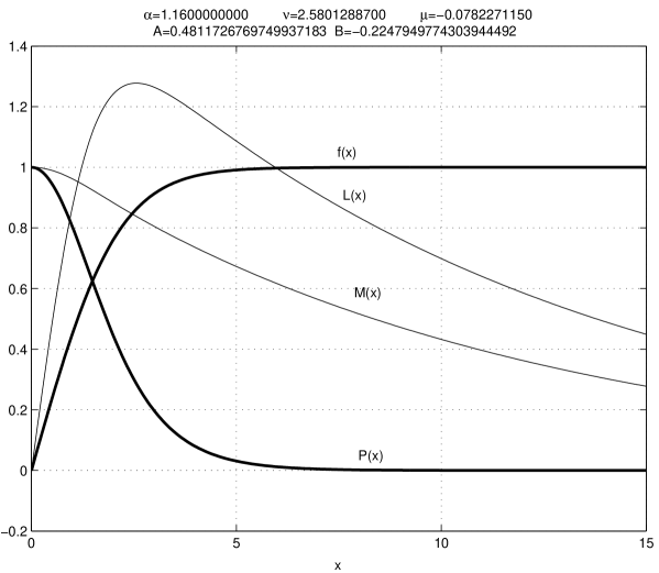
FIG. 1.: A vortex-like solution of the Abelian-Higgs model leading to gravity localization.

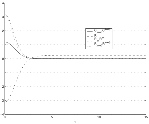
FIG. 2.: The curvature invariants in the case of the solution given in Fig. 1.

Consider now the parameter set leading to the regular solution reported in Fig. 1 where $\epsilon=0$. If we now change continuously $\epsilon$ from $\epsilon=0$ to $\epsilon>0$ new solutions (still regular) can be found by tuning the other parameters of the original solution to the new value of $\epsilon$. More precisely, at least one of the three original parameters [i.e. $\alpha$, $\mu$, $\nu$] should be adapted to the new value of $\epsilon$. In this way new regular solutions can be found. The results of the numerical integration and the corresponding curvature invariants are reported in Fig. 3 and Fig. 4 for the case $\epsilon=1$. The solution of Figs. 3 and 4 are obtained from the solution reported in Figs. 1 and 2 by adapting the parameters according to the procedure outlined above. The amount of tuning can be appreciated by comparing the values of $\alpha$, $\mu$ and $\nu$ given in Fig. 1 with the ones given in Fig. 3.

The value of $\epsilon=1$ (corresponding to the integrations reported in Figs. 3 and 4 ) is only illustrative and similar solutions can be found for other values of $\epsilon$. Notice, however, that since $\mu<0$ and $\epsilon>0$ it should always happen that

$$\epsilon<\frac{5}{12|\mu|},$$ (5.1)

since only in this case the bulk solutions discussed in Eqs. (3.7)–(3.8) are not imaginary.

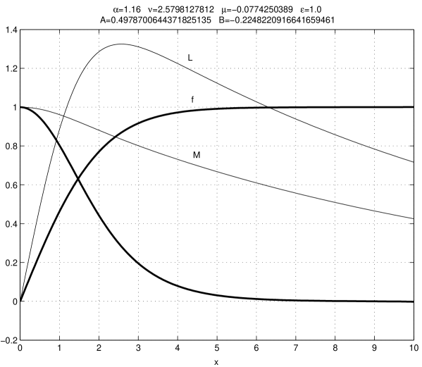
FIG. 3.: A regular solution for $\epsilon>0$ is illustrated. The parameters of the solution are the ones of Fig. 1 but adapted to the new value of $\epsilon$, i.e. $\epsilon=1$.

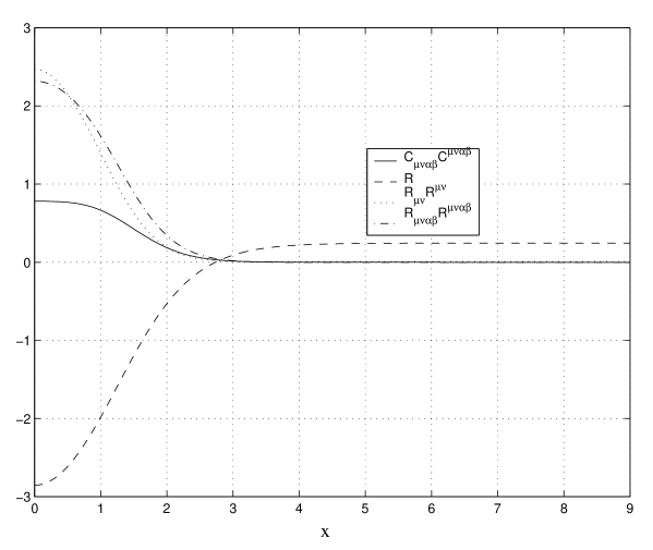
FIG. 4.: The curvature invariants in the case of the solution given in Fig. 3.

Consider now the case when a given solution is divergent in the absence of curvature corrections. It will now be shown that if EGB self-interactions are included the singular solutions are regularized provided the value of $\epsilon$ is appropriately selected.

In the case $\epsilon=0$ the parameter space of the solution is represented by a surface in the $(\alpha,\nu,\mu)$ plane. When the parameters lie on this surface, warped solutions leading to gravity localization can be found. An example of such a surface is given in Fig. 5.

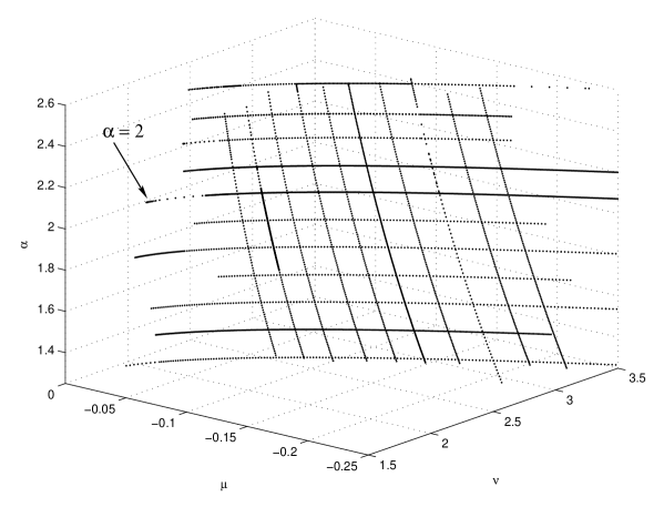
FIG. 5.: The parameter space of the solution in the case $\epsilon=0$. The curve $\alpha=2$ is also indicated.

Let us now focus the attention on a point which lies outside of the fine-tuning surface. In this case the geometry gets singular. More specifically, two independent solutions can be found. These solutions have divergent curvature invariants for a finite value of $x$ which we call $x_{0}$. For $x<x_{0}$ the solution has two branches and can be parametrized as

$$M(x)\sim(x_{0}-x)^{\gamma},\,\,\,{\cal L}(x)\sim(x_{0}-x)^{\delta},$$ (5.2)

with

$$4\gamma+\delta=1,\,\,\,\,4\gamma^{2}+\delta^{2}=1.$$ (5.3)

These solutions are nothing but the well known Kasner solutions, widely discussed in cosmological frameworks and in the context of gravitational collapse. The Kasner conditions leave open only two possibilities: either $\delta=1$ and $\gamma=0$ or $\gamma=2/5$ and $\delta=-3/5$. The branch with $\delta=1$ leads only to a coordinate singularity whereas the other branch leads to a curvature singularity.

For sake of clarity consider the case when $\alpha=2$. In this case the parameter space of the solution $\epsilon=0$ reduces to a curve in the ($\mu$,$\nu$) plane where $\alpha$ is constant (and fixed to $2$). This curve is indicated with an arrow in Fig. 5.

Let us now take values of $\mu$ and $\nu$ outside of the fine-tuning surface in the case $\alpha=2$. Then, as argued, a singular solution appears. In fact, in Fig. 6, $M(x)$ goes to zero and ${\cal L}(x)$ blows up according to the Kasnerian relations.

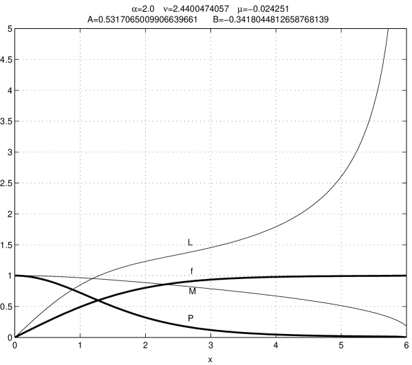
FIG. 6.: A singular solution outside the fine-tuning surface for $\epsilon=0$.

The curvature invariants for the solution of Fig. 6 are reported in Fig. 7.

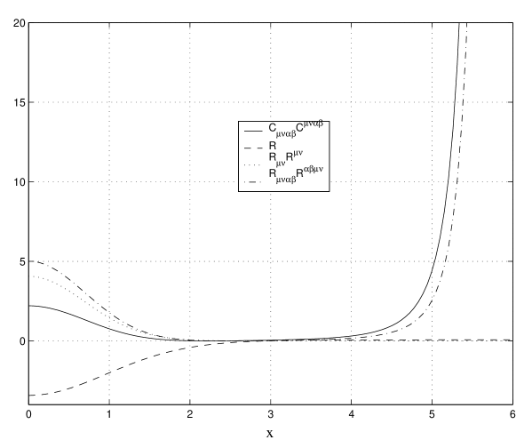
FIG. 7.: The curvature invariants for the solution given in Fig. 6.

Figs. 6 and 7 are obtained for $\epsilon=0$. It is now possible to integrate the system in the case when $\epsilon\neq 0$. By tuning the value of $\epsilon$ the singular solution can be regularized. The results of this analysis are reported in Figs. 8 and 9.

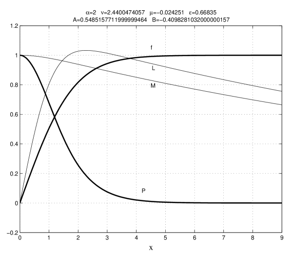
FIG. 8.: A regularized solution. The parameters are exactly the ones given in Fig. 6 except for $\epsilon$ which is zero in Fig. 6.

The curvature invariants for the solution of Fig. 7 are reported in Fig. 9.

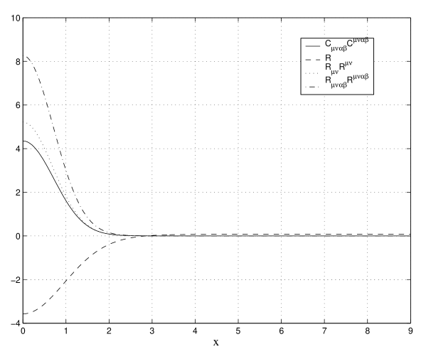
FIG. 9.: The curvature invariants for the solution given in Fig. 8.

This example is representative of a more general feature of the model. If a solution is singular for $\epsilon=0$, it can be regularized for by adapting the value of $\epsilon$. If $\epsilon\neq 0$ the parameter space of regular solutions leading to warped compactification is wider than in the case $\epsilon=0$. This aspect will be further analyzed in Section V.

B Solutions with $\Lambda>0$.

From the analysis of Eqs. (3.7) and (3.8), it is clear that regular solutions where $\mu>0$ and $\epsilon<0$ cannot be obtained. Hence, let us discuss the case where $\mu>0$ and $\epsilon>0$. We are primarily interested in solutions of the equations of motion describing a vortex in a six-dimensional regular geometry with warp factors exponentially decreasing at infinity. A general argument will now show that these solutions are not possible if the cosmological constant is positive and $\epsilon>0$.

If the solutions shall describe exponentially decreasing warp factors for large $x$, then $m(x)$ should decrease reaching, asymptotically, a constant negative value. This value is determined by the bulk solutions and it is given, in the case $\mu>0$ and $\epsilon>0$ by

$$m_{\infty}=-\sqrt{\frac{1}{12\epsilon}\biggl{(}1+\sqrt{1+\frac{12}{5}\epsilon\mu}\biggr{)}}.$$ (5.4)

Notice now, that, from the equations of motion, a critical point can be defined. It is the point where the function $(1-12\epsilon m^{2})^{-1}$ appearing in Eq. (3.1) blows up:

$$m_{s}=-\frac{1}{\sqrt{12~{}\epsilon}}.$$ (5.5)

If $m(x)$ should decrease from $x=0$ towards negative values reaching, ultimately, $m_{\infty}$, it is easy to see that $m(x)$ should always pass trough $m_{s}$. For this it is enough to notice, from Eq. (5.4), that in spite of the magnitude of $\mu\epsilon$

$$|m_{\infty}|>|m_{s}|.$$ (5.6)

From Eq. (4.16) we have

$$(m-\ell)(1-12\epsilon m^{2})=\frac{\nu}{\alpha}\frac{PP^{\prime}}{{\cal L}^{2}}.$$ (5.7)

Hence, at the point $x_{s}$ where $m=m_{s}$ we will have that

$$\left.\frac{PP^{\prime}}{{\cal L}^{2}}\right|_{x_{s}}=0,$$ (5.8)

and $(m(x_{s})-\ell(x_{s}))$ is finite. So, in $x_{s}$ either $P^{\prime}(x_{s})=0$ or $P(x_{s})=0$. Let us examine, separately, the two cases. Consider, first the case $P^{\prime}(x_{s})=0$ and assume that $m(x)$ and $\ell(x)$ are non singular around $x_{s}$. In this case $m(x)$ and $\ell(x)$ can be expanded in a Taylor series around $x_{s}$. Looking at the difference between Eq. (2.17) and Eq. (2.15)

$$(1-12\epsilon m^{2})\biggl{[}m(l-m)-m^{\prime}\biggr{]}=\frac{\nu}{4}\biggl{(}{f^{\prime}}^{2}-\frac{f^{2}P^{2}}{L^{2}}\biggr{)},$$ (5.9)

we have that, for $x\simeq x_{s}$

$$\biggl{(}{f_{s}^{\prime}}^{2}-\frac{f_{s}^{2}P_{s}^{2}}{L_{s}^{2}}\biggr{)}=0$$ (5.10)

which also implies that $f^{\prime}_{s}\simeq f_{s}P_{s}/L_{s}$. Looking now, separately, at Eqs. (2.17) and (2.15) we see that

$$\tau_{\rho}(x_{s})\simeq\tau_{\theta}(x_{s})\sim-\frac{1}{\nu}\biggl{(}\mu+\frac{5}{12\epsilon}\biggr{)}=-\Omega.$$ (5.11)

Since $\mu$ and $\epsilon$ are both positive, $\Omega>0$. But this leads us to a contradiction since we should have:

$$\tau_{\rho}(x_{s})+\tau_{\theta}(x_{s})=-2\Omega=\frac{1}{2}(f_{s}^{2}-1)^{2}-\frac{{P_{s}^{\prime}}^{2}}{\alpha L_{s}^{2}}.$$ (5.12)

By hypothesis $P^{\prime}_{s}=0$. Hence $(f_{s}^{2}-1)^{2}=-4\Omega$. But $\Omega>0$ and $(f_{s}^{2}-1)^{2}$ is positive definite. This proves that $m(x)$ cannot be regular around $x_{s}$ since the equations of motion lead to a contradiction.

Consider now the case $P_{s}=0$. In this case $P^{\prime}_{s}$ can be either positive or negative. If $P^{\prime}_{s}<0$, this means that $P(x)$ is zero in $x_{s}$ and that it decreases getting more and more negative. However, from Eq. (3.11), $P(x)$ should go to zero at infinity. Hence, $P^{\prime}(x)$ should change sign for $x>x_{s}$. By continuity there should be a point $x_{1}$ where $P^{\prime}(x_{1})=0$ and $P(x_{1})<0$. From Eq. (2.14) we see that this would imply $P^{\prime\prime}(x_{1})<0$ which is not consistent with a minimum in $x_{1}$. But then, if $P_{s}=0$ and $P_{s}^{\prime}<0$ the boundary values of Eq. (3.11) cannot be connected continuously with the behaviour in the core. A similar demonstration can be obtained in the case $P_{s}=0$ and $P^{\prime}_{s}>0$.

VI The parameter space of the solutions

In the previous Section we discussed examples where singular solutions are regularized in the presence of the EGB term. In this Section the parameter space of the solution will be discussed. It will be shown how the presence of quadratic corrections allows to enlarge the parameter space.

In order to do this let us fix one of the three parameters $(\alpha,\mu,\nu)$ and let us see what happens to the parameter space when $\epsilon\neq 0$. Suppose, for instance, that $\alpha$ is fixed. Consider, for consistency with the examples of Secion IV, the case when $\alpha=2$. This case corresponds to the Bogomol’nyi limit [40]. In the case $\epsilon=0$ the fine-tuning curve is illustrated in Fig. 5. In Fig. 10 the parameter space is studied in the case $\epsilon\neq 0$ for $\alpha=2$. The “parabola” appearing in Fig. 10 represents the parameter space of the solution for $\alpha=2$ and $\epsilon=0$. On the almost vertical lines, $\epsilon$ changes.

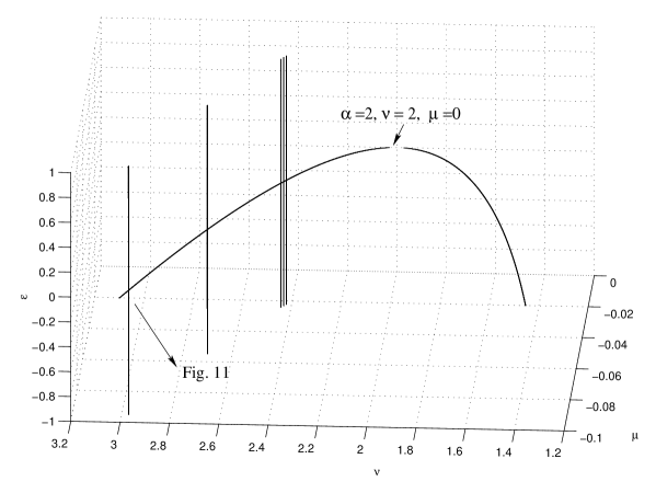
FIG. 10.: The parameter space of the solution is illustrated for the case $\epsilon\neq 0$.

The lines appearing in Fig. 10 are, indeed, not truly vertical. This aspect is illustrated in Fig. 11 where the projection of one of the lines of Fig. 10 is reported for constant $\mu$.

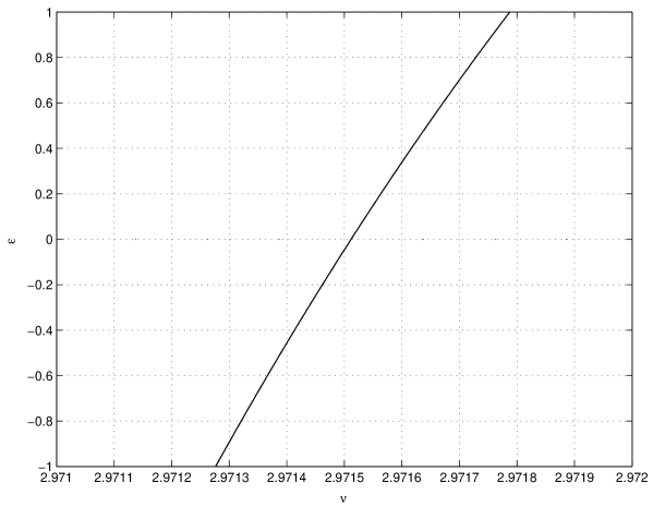
FIG. 11.: The projection, in the $(\epsilon,\nu)$ plane, of the curve with largest $\mu$ appearing in Fig. 10.

The points slected outside the “parabola” would lead, in the absence of quadratic corrections, to singular solutions, as discussed in Section IV. However, if quadratic corrections are present, the parameters of the solution can be adapted to the non-vanishing value of $\epsilon$. In this way, new regular solutions can be found if $\epsilon$ stays on the curves intercepting the “parabola” lying, in its turn, on the $(\mu,\nu)$ plane.

From a practical point of view the various curves intercepting the “parabola” have been obtained in the following way. Starting from the point on the “parabola”, $\mu$ was held constant, $\epsilon$ was varied by small steps and $\nu$ was tuned so that the relation $B=-nu/2alpha$ stays satisfied.

The possibility of finding these regular solutions means that the parameter space is wider in the case when $\epsilon\neq 0$ than in the case when $\epsilon=0$. The same kind of analysis can be numerically performed starting from any point lying on the “parabola” and the five curves reported are only illustrative. As previously stressed, the curves intercepting the “parabola” cannot be extended to arbitrary large values of $\epsilon>0$. In fact, since $\mu<0$ and $\epsilon>0$, from Eqs. (3.7)–(3.8) we must have that $\epsilon<5/(12|\mu|)$ in order to avoid imaginary warp factors.

In Fig. 11 also positive values of $\mu$ have been included. As discussed in the previous Section, expoenentially decreasing solutions for the warp factors are not possible if $\mu$. Moreover, also in the case $\epsilon=0$ exponentially decreasing warp factors are not allowed. The part of the curve corresponding to $\mu>$ leads, for $\epsilon=0$ to exponentially increasing warp factors, as discussed in [15]. The border point between the regions $\mu<0$ and $\mu>0$ of the parameter space is represented by the Bogomol’nyi point where $\mu=0$, $\nu=2$ and $\alpha=2$ [15].

In the case when quadratic curvature corrections are absent the parameter space of the model is three-dimensional and it can be described with a three dimensional plot as in Fig. (5). If quadratic curvature corrections are present the parameter space is four-dimensional and it has to be studied, necessarily, one of the four parameters. In the present discussion $\alpha$ has been fixed. However, the same study can be repeated by fixing either $\mu$ or $\nu$ and by discussing, respectively, the picture of the parameter space in the ($\alpha$, $\nu$, $\epsilon$) or ($\alpha$, $\mu$, $\epsilon$) planes.

VII Concluding remarks

In this paper the solutions of the gravitating Abelian-Higgs model in six-dimensions have been studied. Provided the quadratic corrections are parametrized in the EGB form, new classes of regular solutions leading to warped geometries have been found. The rationale for these results stems from the fact that the relations among the string tensions still exist even if curvature self-interactions are present. In its turn, this property, relies, ultimately, on the features of the EGB combination which does not produce, in the equations of motion, derivatives higher than second.

If the bulk cosmological constant is negative the results of adding the EGB term in the bulk action can be viewed in two different perspectives. Starting from a regular solution (without quadratic corrections), new solutions (still regular) can be found in the vicinity of the initial solution by changing $\epsilon$ from $0$ to $\epsilon>0$. If, in another perspective, we start from a singular solutions (without quadratic corrections) new (regular) solutions can be found by tuning appropriately the value of $\epsilon$.

The results obtained in this investigation show that vortex-like solutions, obtained using the Einstein-Hilbert action, are stable towards the introduction of quadratic corrections of the EGB form. Furthermore, our results suggest that in the parameter space of the regular solutions a new direction opens up when $\epsilon\neq 0$.

The singularity-free solutions discussed in the present paper represent an ideal framework in order to check for the localization of the various modes of the geometry as discussed in [41, 42]. The presence of an (Abelian) gauge field background makes these solutions also rather interesting from the point of view of fermion localization [39]. These problems are left for future studies.

REFERENCES

- [1] V. Rubakov and M. Shaposhnikov, Phys. Lett. B 125, 136 (1983).
- [2] V. Rubakov and M. Shaposhnikov, Phys. Lett. B 125, 139 (1983).
- [3] K. Akama, in Proceedings of the Symposium on Gauge Theory and Gravitation, Nara, Japan, eds. K. Kikkawa, N. Nakanishi and H. Nariai, (Springer-Verlag, 1983), [hep-th/0001113].
- [4] M. Visser, Phys. Lett. B 159 (1985) 22.
- [5] L. Randall and R. Sundrum, Phys. Rev. Lett. 83 3370 (1999).
- [6] L. Randall and R. Sundrum, Phys. Rev. Lett. 83, 4690 (1999).
- [7] N. Mavromatos and J. Rizos, Phys. Rev. D 62, 124004 (2000).
- [8] J. E. Kim, B. Kyae, and H. M. Lee, Nucl. Phys. B 582, 296 (2000); B 591, 587(E) (2000); I. Low and A. Zee, ibid. B 585, 395 (2000).
- [9] S. Nojiri and S. D. Odintsov, J. High Energy Phys. 07, 49 (2000); S. Nojiri, O. Obregon, S. D. Odintsov, Phys.Rev.D 62, 104003 (2000).
- [10] K. A. Meissner, M. Olechowski, [hep-th/0106203].
- [11] I. P. Neupane, JHEP 0009, 040 (2000); I. P. Neupane [hep-th/0106100].
- [12] D. Lovelock, J. Math. Phys. 12, 498 (1971).
- [13] J. Madore, Phys. Lett. 110A, 289 (1985); 111A, 283 (1985).
- [14] M. Henningson and K. Skenderis, JEHEP 9807, 023 (1998); V. Balasubramanian and P. Kraus, Commun. Math. Phys. 208, 413 (1999).
- [15] M. Giovannini, H. Meyer, and M. Shaposhnikov, hep-th/0104118.
- [16] T. Gherghetta and M. Shaposhnikov, Phys. Rev. Lett. 85, 353 (2000).
- [17] A. G. Cohen and D. B. Kaplan, Phys. Lett. B 470, 52 (1999).
- [18] A. Chodos and E. Poppitz, Phys. Lett. B 471, 119 (1999).
- [19] I. Olasagasti and A. Vilenkin, Phys. Rev. D 62, 044014 (2000).
- [20] R. Gregory, Phys. Rev. Lett. 84, 2564 (2000).
- [21] S.-H. Moon, S.-J. Rey, and Y.-B. Kim, hep-th/0012165.
- [22] G. Dvali, hep-th/0004057.
- [23] T. Gherghetta, E. Roessl, M. Shaposhnikov, Phys.Lett.B 491 (2000) 353.
- [24] S. Randjbar-Daemi, A. Salam and J. Strathdee, Phys. Lett. B 132 (1983) 56.
- [25] S. Randjbar-Daemi and M. Shaposhnikov, Phys. Lett. B 492 (2000) 361.
- [26] S. Randjbar-Daemi and M. Shaposhnikov, Phys. Lett. B 491 (2000) 329.
- [27] R. Gregory and A. Padilla, hep-th/0107108.
- [28] N. Arkani-Hamed, S. Dimopoulos, G. Dvali, Phys.Lett.B 429, 263 (1998).
- [29] I. Antoniadis, N. Arkani-Hamed, S. Dimopoulos, G. Dvali, Phys.Lett. B 436, 257 (1998).
- [30] I. Antoniadis, S. Dimopoulos, G. Dvali Nucl.Phys.B 516, 70 (1998).
- [31] H.B. Nielsen and P. Olesen, Nucl. Phys.B 61, 45 (1973).
- [32] M. Giovannini, Phys. Rev. D 63, 085005 (2001).
- [33] M. Giovannini, Phys. rev. D 63, 064011 (2001).
- [34] B. Zwiebach, Phys. Lett. 156B, 315 (1985).
- [35] D. G. Boulware and S. Deser, Phys. Rev. Lett. 55, 2656 (1985); Phys. Lett. 175B, 409 (1986).
- [36] R. R. Metsaev and A. A. Tseytlin, Phys. Lett. 191B, 115 (1987); Nucl. Phys. B293, 385 (1987).
- [37] C. G. Callan, E. J. Martinec, M. J. Perry, and D. Friedan, Nucl. Phys. B 262, 593 (1985).
- [38] A. Sen, Phys. Rev. Lett. 55, 1846 (1985).
- [39] M.V. Libanov and S.V. Troitsky Nucl. Phys. B 599, 319 (2001); J. M. Frere, M.V. Libanov and S.V. Troitsky, hep-ph/0012306.
- [40] E. B. Bogomol’nyi, Sov. J. Nucl. Phys. 24 (1976) 449 [ Yad. Fiz. 24 (1976) 861].
- [41] M. Giovannini, hep-th/0106041 (Phys. Rev. D, in press); hep-th/0106131.
- [42] M. Giovannini, hep-th/0107233.