Scattering amplitude and shift in self-energy in medium

S. Mallik***Permanent address : Saha Institute of Nuclear Physics, 1/AF, Bidhannagar, Calcutta-700064, India Institute for Theoretical Physics, University of Bern, Sidlerstrasse 5, CH-3012 Bern, Switzerland
Abstract

Two simple proofs are presented for the first order virial expansion of the self-energy of a particle moving through a medium, characterised by temperature and/or chemical potential(s). One is based on the virial expansion of the self-energy operator itself, while the other is on the analysis of its Feynman diagrams in configuration space.

I Introduction

More than a decade ago, Leutwyler and Smilga [1] considered the problem of mass-shift and damping rate of a nucleon propagating through a heat bath. As one of the methods to deal with the problem, they wrote (the first term of) the virial expansion of the nucleon self-energy, which relates it to the pion-nucleon scattering amplitude in the forward direction. At low pion density the first order formula yields the dominating contribution. The advantage of such a formula is that one can use the experimental data to compute the shift in self-energy without relying on any theoretical structure. Further the formula is simple enough to suggest a generalisation to other hadrons in different media. Accordingly a number of authors have used these relations to explore the properties of hadrons in such media [2, 3, 4].

In the context of quantum electrodynamics, Barton [5] took a physical approach to derive such formulae, following an earlier suggestion by Feynman [6]. The refractive index of a medium for a beam of particles of a definite frequency differs from unity due to the scattering of the incident beam by particles of the medium. The change in frequency (energy) of the particles may be related to this change in refractive index. In this way Feynman related the self-energy of the electron to its forward scattering amplitude with the virtual quanta in vacuum. Barton extended these considerations to the black body radiation.

Recently the complete expansion of the self-energy in the medium in powers of the distribution function has been proven in perturbation theory [7]. In effect, it is a reordering of the contributions in perurbation theory, which is an expansion in powers of coupling contant, to one in powers of the distribution function. The analysis is carried out in imaginary time formulation of field theory in the medium.

Here we present two simple proofs of the first term in the expansion of the self-energy. One is a generalisation of the method used in Ref.[8] and is based directly on the virial expansion of the ensemble average of any operator. The other is in perturbation theory, based on Feynman diagrams in configuration space.

We shall work here in the real time formulation of field theory at finite temperature and density. Secs. II and III describe the two proofs of the virial expansion. Sec. IV discusses the relevance of such formulae and possibility of extending the proofs to higher order.

II Virial expansion

Following Weinberg [9], we introduce a compact notation for different types particles and their fields. Let $a(\vec{p},\sigma,f)$ and a†​(pβ†’,Οƒ,f)superscriptπ‘Žβ€ β†’π‘πœŽπ‘“a^{{\dagger}}(\vec{p},\sigma,f) be the destruction and creation operators for a particle of species $f$ having momentum $\vec{p}$ and spin projection $\sigma$; then for example,


|pβ†’,Οƒ,f⟩=a†​(pβ†’,Οƒ,f)​|0⟩.ketβ†’π‘πœŽπ‘“superscriptπ‘Žβ€ β†’π‘πœŽπ‘“ket0\displaystyle|\vec{p},\sigma,f\rangle=a^{{\dagger}}(\vec{p},\sigma,f)|0\rangle.

They satisfy the commutation (anticommutation) relations $(\omega_{p}=\sqrt{\vec{p}\,^{2}+m^{2}})$,


$\displaystyle[a(\vec{p},\sigma,f),a^{{\dagger}}(\vec{p}\,^{\prime},\sigma^{\prime},f^{\prime}]_{\mp}=(2\pi)^{3}2\omega_{p}\delta^{3}(\vec{p}-\vec{p}\,^{\prime})\delta_{\sigma\sigma^{\prime}}\delta_{ff^{\prime}}.$

The field operators are denoted by $\psi_{l}(x)$, where the index $l$ denotes not only the field type but also runs over its components. Then $\psi_{l}(x)$ may be expanded as

ψl​(x)=βˆ‘Οƒβˆ«d3​p(2​π)3​12​ωp​[ul​(pβ†’,Οƒ,f)​a​(pβ†’,Οƒ,f)​eβˆ’i​pβ‹…x+vl​(pβ†’,Οƒ,f)​a†​(pβ†’,Οƒ,fc)​ei​pβ‹…x],subscriptπœ“π‘™π‘₯subscript𝜎superscript𝑑3𝑝superscript2πœ‹312subscriptπœ”π‘delimited-[]subscriptπ‘’π‘™β†’π‘πœŽπ‘“π‘Žβ†’π‘πœŽπ‘“superscript𝑒⋅𝑖𝑝π‘₯subscriptπ‘£π‘™β†’π‘πœŽπ‘“superscriptπ‘Žβ€ β†’π‘πœŽsuperscript𝑓𝑐superscript𝑒⋅𝑖𝑝π‘₯\psi_{l}(x)=\sum_{\sigma}\int{d^{3}p\over{(2\pi)^{3}}}{1\over{2\omega_{p}}}\left[u_{l}(\vec{p},\sigma,f)a(\vec{p},\sigma,f)e^{-ip\cdot x}+v_{l}(\vec{p},\sigma,f)a^{{\dagger}}(\vec{p},\sigma,f^{c})e^{ip\cdot x}\right], (1)

$f^{c}$ denoting the antiparticle of the species $f$. The coefficient functions $u_{l}$ and $v_{l}$ depend on the spin of the particle. We have in mind the three types of fields, namely, the scalar field $\phi(x)$ for which $u_{l}=v_{l}=1$; the Dirac spinor field $\psi(x)$, for which they are the normalised Dirac spinors, $\bar{u}(\vec{p},\sigma)u(\vec{p},\sigma)=-\bar{v}(\vec{p},\sigma)v(\vec{p},\sigma)=2m$ and the vector field $A_{\mu}$, for which they are the polarisation vectors, $\epsilon_{\mu}(\vec{p},\sigma),\,\epsilon_{\mu}^{*}(\vec{p},\sigma)\epsilon^{\mu}(\vec{p},\sigma^{\prime})=-\delta_{\sigma\sigma^{\prime}}$. Below we shall in most places suppress the variable $\sigma$ of $u_{l},\,v_{l},\,a\,$ and a†superscriptπ‘Žβ€ a^{{\dagger}}. If there is an integration over a 3-momentum, a summation over the corresponding $\sigma$ as in Eq (2.1) will also be implied.

In the real time formulation of field theory in medium, all Greens functions, in particular the self-energy, acquire a $2\otimes 2$ matrix structure. Since we confine here only to contributions linear in the distribution function, it will, however, suffice to consider only the 11-component of these matrices. Below we shall drop the 11 index 111 The self-energy function $\Sigma$ which actually shifts the pole position of the propagator is related to the components in a simple way [10]. With $\Sigma_{11}$ these relations are, $Re\Sigma(p)=Re\Sigma_{11}(p)$ and $Im\Sigma(p)=\alpha Im\Sigma_{11}(p)$, where $\alpha=tanh(\beta p_{0}/2)$ for bosons and $\alpha=coth\{\beta(p_{0}-\mu)/2\}$ for fermions ($p_{o}>0)$. Thus $\Sigma_{11}$ deviates from $\Sigma$ by exponential corrections at small temperatures. Further the factor $\alpha$ actually cancels on rearranging the distribution functions within the integral, at least for 1-loop contributions [11]..

Let us begin with the self-energy $\Sigma_{f}^{(0)}(p)$ of a particle of type $f$ and momentum $p$ in vacuum. For our purpose, we write this amputated, two-point Green’s function as

βˆ’i​(2​π)4​δ4​(pβ€²βˆ’p)​uΒ―l​(pβ†’,f)​Σf(0)​(p)​ul​(pβ†’,f)=⟨0|a​(pβ†’β€²,f)​(Sβˆ’1)​a†​(pβ†’,f)|0⟩,𝑖superscript2πœ‹4superscript𝛿4superscript𝑝′𝑝subscript¯𝑒𝑙→𝑝𝑓superscriptsubscriptΣ𝑓0𝑝subscript𝑒𝑙→𝑝𝑓quantum-operator-product0π‘Žsuperscript→𝑝′𝑓𝑆1superscriptπ‘Žβ€ β†’π‘π‘“0-i(2\pi)^{4}\delta^{4}(p^{\prime}-p)\bar{u}_{l}(\vec{p},f)\Sigma_{f}^{(0)}(p)u_{l}(\vec{p},f)=\langle 0|a(\vec{p}\,^{\prime},f)(S-1)a^{{\dagger}}(\vec{p},f)|0\rangle, (2)

where the $S$-operator is given by the familiar time ordered expression,


$\displaystyle S=Te^{i\int d^{4}x{{\cal L}_{I}}(x)},$

${{\cal L}_{I}}(x)$ being any interaction Lagrangian built out of the fields $\psi_{l}(x)$. Because $\Sigma_{f}^{(0)}(p)$ is one-particle irreducible by definition, it is understood here and below that we only retain such diagrams in matrix elements like the one on the right hand side of Eq.(2.2). The corresponding self-energy in the medium will be denoted by ${\Sigma}_{f}(p,u)$, where $u^{\mu}$ is the 4-velocity of the medium 222 No confusion should arise from the use of same $u$ in both $u^{\mu}$ and $u_{l}(\vec{p},f)$.. Actually we shall work in the rest frame of the medium $(u^{0}=1,\,\vec{u}=0)$. Then we may write

βˆ’i​(2​π)4​δ4​(pβ€²βˆ’p)​uΒ―l​(pβ†’,f)​Σf​(p,u)​ul​(pβ†’,f)=⟨a​(pβ†’β€²,f)​(Sβˆ’1)​a†​(pβ†’,f)⟩,𝑖superscript2πœ‹4superscript𝛿4superscript𝑝′𝑝subscript¯𝑒𝑙→𝑝𝑓subscriptΣ𝑓𝑝𝑒subscript𝑒𝑙→𝑝𝑓delimited-βŸ¨βŸ©π‘Žsuperscript→𝑝′𝑓𝑆1superscriptπ‘Žβ€ β†’π‘π‘“-i(2\pi)^{4}\delta^{4}(p^{\prime}-p)\bar{u}_{l}(\vec{p},f){\Sigma}_{f}(p,u)u_{l}(\vec{p},f)=\langle a(\vec{p}\,^{\prime},f)(S-1)a^{{\dagger}}(\vec{p},\ f)\rangle, (3)

where $\langle\cdots\rangle$ denotes ensemble average: For any operator $O$,

$$\langle O\rangle=Tr(\rho O),\qquad\rho=e^{-\beta(H-\mu{\cal N})}/Tre^{-\beta(H-\mu{\cal N})}.$$ (4)

Here $H$ is the Hamiltonian, $\beta^{-1}$ the temperature. For illustration we include a chemical potential $\mu$ for a fermionic species with the corresponding number operator ${\cal N}$.

The ensemble average $\langle O\rangle$ admits a virial expansion

$$\langle O\rangle=\langle 0|O|0\rangle+\sum_{f^{\prime}}\int{d^{3}k\over{(2\pi)^{3}2\omega_{k}}}n_{f^{\prime}}(\omega_{k})\langle\vec{k},f^{\prime}|O|\vec{k},f^{\prime}\rangle+\cdots,$$ (5)

where the sum over $f^{\prime}$ runs in general over the species of particles present in the medium. The dots represent terms of higher order in the distribution function $n$. The latter are given by the familiar expressions, $n_{B}(\omega_{k})=(e^{\beta\omega_{k}}-1)^{-1}$ for bosons and $n_{F}^{\pm}(\omega_{k})=(e^{\beta(\omega_{k}\mp\mu)}+1)^{-1}$ for fermions and antifermions respectively. Applying Eq.(2.5) to the left hand side of Eq.(2.3), we get for $\tilde{\Sigma}_{f}(p,u)\equiv{\Sigma}_{f}(p,u)-\Sigma_{f}^{(0)}(p)$,

βˆ’i​(2​π)4​δ4​(pβ€²βˆ’p)​uΒ―l​(pβ†’,f)​Σ~f​(p,u)​ul​(pβ†’,f)=βˆ‘fβ€²βˆ«d3​k(2​π)3​2​ωk​nf′​(Ο‰k)β€‹βŸ¨kβ†’,fβ€²|a​(pβ†’β€²,f)​(Sβˆ’1)​a†​(pβ†’,f)|kβ†’,fβ€²βŸ©.𝑖superscript2πœ‹4superscript𝛿4superscript𝑝′𝑝subscript¯𝑒𝑙→𝑝𝑓subscript~Σ𝑓𝑝𝑒subscript𝑒𝑙→𝑝𝑓subscriptsuperscript𝑓′superscript𝑑3π‘˜superscript2πœ‹32subscriptπœ”π‘˜subscript𝑛superscript𝑓′subscriptπœ”π‘˜quantum-operator-productβ†’π‘˜superscriptπ‘“β€²π‘Žsuperscript→𝑝′𝑓𝑆1superscriptπ‘Žβ€ β†’π‘π‘“β†’π‘˜superscript𝑓′-i(2\pi)^{4}\delta^{4}(p^{\prime}-p)\bar{u}_{l}(\vec{p},f)\tilde{\Sigma}_{f}(p,u)u_{l}(\vec{p},f)=\sum_{f^{\prime}}\int{d^{3}k\over{(2\pi)^{3}2\omega_{k}}}n_{f^{\prime}}(\omega_{k})\langle\vec{k},f^{\prime}|a(\vec{p}\,^{\prime},f)(S-1)a^{{\dagger}}(\vec{p},f)|\vec{k},f^{\prime}\rangle. (6)

The matrix element on the right in this equation is recognised to be the amplitude $T$ for scattering of a $f$-particle of momentum $p$ with a $f^{\prime}$-particle of momentum $k$ in the forward direction,

⟨kβ†’,fβ€²|a​(pβ†’β€²,f)​(Sβˆ’1)​a†​(pβ†’,f)|kβ†’,fβ€²βŸ©=i​(2​π)4​δ4​(pβ†’β€²βˆ’pβ†’)​Tf​f′​(p,k).quantum-operator-productβ†’π‘˜superscriptπ‘“β€²π‘Žsuperscript→𝑝′𝑓𝑆1superscriptπ‘Žβ€ β†’π‘π‘“β†’π‘˜superscript𝑓′𝑖superscript2πœ‹4superscript𝛿4superscript→𝑝′→𝑝subscript𝑇𝑓superscriptπ‘“β€²π‘π‘˜\langle\vec{k},f^{\prime}|a(\vec{p}\,^{\prime},f)(S-1)a^{{\dagger}}(\vec{p},f)|\vec{k},f^{\prime}\rangle=i(2\pi)^{4}\delta^{4}(\vec{p}\,^{\prime}-\vec{p})T_{ff^{\prime}}(p,k). (7)

We thus get the virial expansion for the self energy to first order,

$$-\bar{u}_{l}(\vec{p},f)\tilde{\Sigma}_{f}(p,u)u_{l}(\vec{p},f)=\sum_{f^{\prime}}\int{d^{3}k\over{(2\pi)^{3}2\omega_{k}}}n_{f^{\prime}}(\omega_{k})T_{ff^{\prime}}(p,k),$$ (8)

where an average over the polarizations of $f$-species and a sum over the polarizations of the different $f^{\prime}$-species are understood.

We now apply this formula to two cases of interest. The first one is that of a nucleon in a medium. Its complete propagator in the medium is $i/(p\!\!\!/-m-\tilde{\Sigma}_{f})$. For the nucleon at rest $(\vec{p}=0)$ in the rest frame of the medium, we can write $\tilde{\Sigma}_{f}=a+b\gamma^{0}$, getting $\bar{u}(p)\tilde{\Sigma}_{f}u(p)=2m_{N}(a+b)$. Also the complete propagator simplifies to


$\displaystyle{i\over{p_{0}-(m_{N}+a+b)}}\cdot{1\over 2}(1+\gamma^{0})$

. Thus the new pole position is given by [1],

$$\tilde{m}_{N}-{i\over 2}\Gamma_{N}=m_{N}-{1\over 2m_{N}}\sum_{f^{\prime}}\int{d^{3}k\over{(2\pi)^{3}2\omega_{k}}}n(\omega_{k})T_{Nf^{\prime}}(p,k).$$ (9)

The other case we consider is that of a vector meson in the medium. Let us rewrite Eq.(2.8) as

βˆ’13β€‹βˆ‘ΟƒΟ΅ΞΌβˆ—β€‹(p,Οƒ)​Π~μ​ν​(p,u)​ϡν​(p,Οƒ)=βˆ‘fβ€²βˆ«d3​k(2​π)3​2​ωk​nf′​(Ο‰k)​TV​f′​(p,k).13subscript𝜎superscriptsubscriptitalic-Ο΅πœ‡π‘πœŽsuperscript~Ξ πœ‡πœˆπ‘π‘’subscriptitalic-Ο΅πœˆπ‘πœŽsubscriptsuperscript𝑓′superscript𝑑3π‘˜superscript2πœ‹32subscriptπœ”π‘˜subscript𝑛superscript𝑓′subscriptπœ”π‘˜subscript𝑇𝑉superscriptπ‘“β€²π‘π‘˜-{1\over 3}\sum_{\sigma}\epsilon_{\mu}^{*}(p,\sigma)\tilde{\Pi}^{\mu\nu}(p,u)\epsilon_{\nu}(p,\sigma)=\sum_{f^{\prime}}\int{d^{3}k\over{(2\pi)^{3}2\omega_{k}}}n_{f^{\prime}}(\omega_{k})T_{Vf^{\prime}}(p,k). (10)

The free propagator for the vector meson is

$$D^{(0)}_{\mu\nu}(p)=\left(-g_{\mu\nu}+{p_{\mu}p_{\nu}\over{m_{V}^{2}}}\right){i\over{p^{2}-m_{V}^{2}}}$$ (11)

To sum the series of 1-particle reducible insertions of the polarisation tensor, we have to decompose the latter in terms of kinematic covariants,

Ξ ~μ​ν=Pμ​ν​Πt+Qμ​ν​Πl,subscript~Ξ πœ‡πœˆsubscriptπ‘ƒπœ‡πœˆsubscriptΠ𝑑subscriptπ‘„πœ‡πœˆsubscriptΠ𝑙\tilde{\Pi}_{\mu\nu}=P_{\mu\nu}\Pi_{t}+Q_{\mu\nu}\Pi_{l}, (12)

which we choose as

$$P_{\mu\nu}=-g_{\mu\nu}+{p_{\mu}p_{\nu}\over p^{2}}-{p^{2}\over\bar{p}^{2}}\tilde{u}_{\mu}\tilde{u}_{\nu},\qquad Q_{\mu\nu}={p^{4}\over\bar{p}^{2}}\tilde{u}_{\mu}\tilde{u}_{\nu},$$ (13)

where $\omega=u\cdot p,\,\bar{p}=\sqrt{\omega^{2}-p^{2}}$ and $\tilde{u}_{\mu}=u_{\mu}-\omega p_{\mu}/p^{2}$. The covariants are free from singularities at $p^{2}=0$, but at $\vec{p}=0$, there is a constraint on the two amplitudes,

Ξ t​(p0,pβ†’=0)=p02​Πl​(p0,pβ†’=0).subscriptΠ𝑑subscript𝑝0→𝑝0superscriptsubscript𝑝02subscriptΠ𝑙subscript𝑝0→𝑝0\Pi_{t}(p_{0},\vec{p}=0)=p_{0}^{2}\Pi_{l}(p_{0},\vec{p}=0). (14)

Then the full propagator becomes

Dμ​ν=ip2βˆ’mV2βˆ’Ξ t​Pμ​ν+ip2βˆ’mV2​(1+Ξ l)​Qμ​νmV2subscriptπ·πœ‡πœˆπ‘–superscript𝑝2superscriptsubscriptπ‘šπ‘‰2subscriptΠ𝑑subscriptπ‘ƒπœ‡πœˆπ‘–superscript𝑝2superscriptsubscriptπ‘šπ‘‰21subscriptΠ𝑙subscriptπ‘„πœ‡πœˆsuperscriptsubscriptπ‘šπ‘‰2D_{\mu\nu}={i\over{p^{2}-m_{V}^{2}-\Pi_{t}}}P_{\mu\nu}+{i\over{p^{2}-m_{V}^{2}(1+\Pi_{l})}}{Q_{\mu\nu}\over m_{V}^{2}} (15)

Thus in general the transverse and the longitudinal components suffer different shifts in the position of the pole. But for the vector meson at rest $(\vec{p}=0)$ the two shifts coincide, because of the constraint equation. We then get the same formula for the pole shift as Eq.(2.9) with the subscript $N$ replaced by $V$.

III Perturbation expansion

We now attempt a perturbative proof of Eq.(2.8). We begin by expanding the $S$-operator in Eq.(2.3) in the familiar perturbation series,

$$-i(2\pi)^{4}\delta^{4}(p^{\prime}-p)\bar{u}_{l}(\vec{p},f){\Sigma}_{f}(p,u)u_{l}(\vec{p},f)=\sum_{N=1}^{\infty}{i^{N}\over{N!}}\int d^{4}x_{1}\cdots d^{4}x_{N}F^{(N)}(x_{1}\cdots x_{N}),$$ (16)

where

F(N)​(x1​⋯​xN)=⟨a​(pβ†’β€²,f)​T​{β„’I​(x1)​⋯​ℒI​(xN)}​a†​(pβ†’,f)⟩paired.superscript𝐹𝑁subscriptπ‘₯1β‹―subscriptπ‘₯𝑁subscriptdelimited-βŸ¨βŸ©π‘Žsuperscript→𝑝′𝑓𝑇subscriptℒ𝐼subscriptπ‘₯1β‹―subscriptℒ𝐼subscriptπ‘₯𝑁superscriptπ‘Žβ€ β†’π‘π‘“pairedF^{(N)}(x_{1}\cdots x_{N})=\langle a(\vec{p}\,^{\prime},f)T\{{{\cal L}_{I}}(x_{1})\cdots{{\cal L}_{I}}(x_{N})\}a^{{\dagger}}(\vec{p},f)\rangle_{\rm paired}. (17)

The subscript ’paired’ indicates that $F^{(N)}$ is the sum of all connected terms obtained by pairing (contracting) all the operators in it in all possible ways. In other words, it represents the sum of all connected Feynman diagrams in the $N$th order. In the following we indicate a pairing by thick dots as superscript. The pairing between a creation or an annihilation operator of a particle with a field operator are given by,

$\displaystyle a^{\bullet}(\vec{p}\,^{\prime},f)\bar{\psi}_{l}^{\bullet}(x)$ $\displaystyle=$ $\displaystyle e^{ip^{\prime}\cdot x}\bar{u}_{l}(\vec{p}\,^{\prime},f)$ (18)
ψlβˆ™β€‹(x)​aβ€ βˆ™β€‹(pβ†’,f)subscriptsuperscriptπœ“βˆ™π‘™π‘₯superscriptsuperscriptπ‘Žβ€ βˆ™β†’π‘π‘“\displaystyle\psi^{\bullet}_{l}(x){a^{{\dagger}}}^{\bullet}(\vec{p},f) $\displaystyle=$ $\displaystyle e^{-ip\cdot x}u_{l}(\vec{p},f).$ (19)

We may choose to work out the self energy of a particle. But the medium may contain antiparticles. So we also note the contractions,

$\displaystyle a^{\bullet}(\vec{p}\,^{\prime},f^{c})\psi_{l}^{\bullet}(x)$ $\displaystyle=$ $\displaystyle e^{ip^{\prime}\cdot x}v_{l}(\vec{p}\,^{\prime},f)$ (20)
ψ¯lβˆ™β€‹(x)​aβ€ βˆ™β€‹(pβ†’,fc)subscriptsuperscriptΒ―πœ“βˆ™π‘™π‘₯superscriptsuperscriptπ‘Žβ€ βˆ™β†’π‘superscript𝑓𝑐\displaystyle\bar{\psi}^{\bullet}_{l}(x){a^{{\dagger}}}^{\bullet}(\vec{p},f^{c}) $\displaystyle=$ $\displaystyle e^{-ip\cdot x}\bar{v}_{l}(\vec{p},f).$ (21)

Finally the pairing of two field operators results in the free propagator in the medium [12],

$$\psi_{l}^{\bullet}(x)\bar{\psi}_{m}^{\bullet}(y)=\langle T\psi_{l}(x)\bar{\psi}_{m}(y)\rangle.$$ (22)

A free propagator in the medium differs from that in vacuum if there are like-particles in the medium. In that case, it has an extra term containing the distribution function $n$ of the particles in the medium and a mass-shell $\delta$-function. Thus, isolating this term amounts to putting the internal line on mass-shell, i.e. opening the propagator into two external lines. When the $\delta$-function is integrated out, this $n$-dependent piece in the propagator, to be denoted by a subscript $n$, becomes,

$$\langle T\psi_{l}(x)\bar{\psi}_{m}(y)\rangle_{n}=\int{d^{3}k\over{(2\pi)^{3}2\omega_{k}}}\left\{\pm n^{+}_{f}(\omega_{k})e^{-ik\cdot(x-y)}u_{l}(\vec{k},f)\bar{u}_{m}(\vec{k},f)+n_{f}^{-}(\omega_{k})e^{ik\cdot(x-y)}v_{l}(\vec{k},f)\bar{v}_{m}(\vec{k},f)\right\},$$ (23)

where + (–) sign before the first term holds if the species $f$ is a boson (fermion). The distribution functions $n^{+}$ and $n^{-}$ coincide if there is no chemical potential.

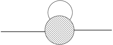
Let us assume, for simplicity, that only one species of particles has its free propagator altered in the medium by the additional term (3.6). We single out this field from the compact notation $\psi_{l}(x)$ and call it $\chi_{l}(x)$ and denote its species by $f^{\prime}$ 333 For self-conjugate species like $\pi^{0}$, the two terms in Eq.(3.6) contribute to the same amplitude, the direct and crossed processes being identical.. We now wish to collect all the linear contributions in $n$ by opening each of the $\chi$-propagators in turn in each of the Feynman diagrams for the self energy in the $N$ th order of its perturbation expansion (Fig. 1). To this end we consider the sum of Feynman diagrams, to be denoted by $F^{(N)}_{ij}(x_{1},\cdots,x_{N})$, containing a $\chi$-propagator between any two vertices, say at $x_{i}$ and $x_{j}$,

Fi​j(N)​(x1,β‹―,xN)=⟨a​(p→′​f)​T​{β„’I​(x1)​⋯​ℒIβˆ™β€‹(xi)​⋯​ℒIβˆ™β€‹(xj)​⋯​ℒI​(xN)}​a†​(pβ†’,f)⟩paired,subscriptsuperscript𝐹𝑁𝑖𝑗subscriptπ‘₯1β‹―subscriptπ‘₯𝑁subscriptdelimited-βŸ¨βŸ©π‘Žsuperscript→𝑝′𝑓𝑇subscriptℒ𝐼subscriptπ‘₯1β‹―superscriptsubscriptβ„’πΌβˆ™subscriptπ‘₯𝑖⋯superscriptsubscriptβ„’πΌβˆ™subscriptπ‘₯𝑗⋯subscriptℒ𝐼subscriptπ‘₯𝑁superscriptπ‘Žβ€ β†’π‘π‘“pairedF^{(N)}_{ij}(x_{1},\cdots,x_{N})=\langle a(\vec{p}\,^{\prime}f)T\{{{\cal L}_{I}}(x_{1})\cdots{{\cal L}_{I}}^{\bullet}(x_{i})\cdots{{\cal L}_{I}}^{\bullet}(x_{j})\cdots{{\cal L}_{I}}(x_{N})\}{a^{{\dagger}}}(\vec{p},f)\rangle_{\rm paired}, (24)

where we explicitly indicate the pairing of the two fields at $x_{i}$ and $x_{j}$.

Consider first the indicated pairing in Eq.(3.7) before any other pairings are carried out, ie, keeping all other operators in their respective positions in the $T$-product. By a certain number of interchanges of the field operators we bring them together to form $\langle\chi_{l}(x_{i})\bar{\chi}_{m}(x_{j})\rangle$. Then we extract its $n$-dependent contribution given by Eq.(3.6) 444If $f^{\prime}$ is a fermionic species, there may be two such propagators between $x_{i}$ and $x_{j}$. We, of course, have to extract this contribution from both of them.. Since we restrict to linear contributions in $n$, we set all other in-medium propagators to their vacuum values.

In order to interpret the resulting expression in terms of a two-body scattering amplitude, we use (3.3) to rewrite the coefficient functions for $f^{\prime}$ species in $\langle\chi_{l}(x_{i})\bar{\chi}_{m}(x_{j})\rangle$ as pairings,

eβˆ’i​kβ‹…(xiβˆ’xj)​ul​(kβ†’,fβ€²)​uΒ―m​(kβ†’,fβ€²)=Ο‡lβˆ™β€‹(xi)​aβ€ βˆ™β€‹(kβ†’,fβ€²)​aβˆ™βˆ™β€‹(kβ†’,fβ€²)​χ¯mβˆ™βˆ™β€‹(xj).superscriptπ‘’β‹…π‘–π‘˜subscriptπ‘₯𝑖subscriptπ‘₯𝑗subscriptπ‘’π‘™β†’π‘˜superscript𝑓′subscriptΒ―π‘’π‘šβ†’π‘˜superscript𝑓′superscriptsubscriptπœ’π‘™βˆ™subscriptπ‘₯𝑖superscriptsuperscriptπ‘Žβ€ βˆ™β†’π‘˜superscript𝑓′superscriptπ‘Žβˆ™absentβˆ™β†’π‘˜superscript𝑓′superscriptsubscriptΒ―πœ’π‘šβˆ™absentβˆ™subscriptπ‘₯𝑗e^{-ik\cdot(x_{i}-x_{j})}u_{l}(\vec{k},f^{\prime})\bar{u}_{m}(\vec{k},f^{\prime})=\chi_{l}^{\bullet}(x_{i}){a^{{\dagger}}}^{\bullet}(\vec{k},f^{\prime})a^{\bullet\bullet}(\vec{k},f^{\prime}){\bar{\chi}}_{m}^{\bullet\bullet}(x_{j}). (25)

For the antiparticle species $f^{\prime c}$, we use Eq.(3.4) to write an analogous equation,

ei​kβ‹…(xiβˆ’xj)​vl​(kβ†’,fβ€²)​vΒ―m​(kβ†’,fβ€²)=aβˆ™β€‹(kβ†’,f′⁣c)​χlβˆ™β€‹(xi)​χmβˆ™βˆ™β€‹(xj)​aβ€ βˆ™βˆ™β€‹(kβ†’,f′⁣c).superscriptπ‘’β‹…π‘–π‘˜subscriptπ‘₯𝑖subscriptπ‘₯𝑗subscriptπ‘£π‘™β†’π‘˜superscript𝑓′subscriptΒ―π‘£π‘šβ†’π‘˜superscript𝑓′superscriptπ‘Žβˆ™β†’π‘˜superscript𝑓′𝑐superscriptsubscriptπœ’π‘™βˆ™subscriptπ‘₯𝑖superscriptsubscriptπœ’π‘šβˆ™absentβˆ™subscriptπ‘₯𝑗superscriptsuperscriptπ‘Žβ€ βˆ™absentβˆ™β†’π‘˜superscript𝑓′𝑐e^{ik\cdot(x_{i}-x_{j})}v_{l}(\vec{k},f^{\prime})\bar{v}_{m}(\vec{k},f^{\prime})=a^{\bullet}(\vec{k},f^{\prime c})\chi_{l}^{\bullet}(x_{i}){\chi}_{m}^{\bullet\bullet}(x_{j}){a^{{\dagger}}}^{\bullet\bullet}(\vec{k},f^{\prime c}). (26)

Now the $\chi$ fields can be brought back to their original positions forming again the complete vertices ${{\cal L}_{I}}(x_{i})$ and ${{\cal L}_{I}}(x_{j})$. We also bring the creation and the annihilation operators respectively to the right and the left of the $T$-product getting

$\displaystyle F^{(N)}_{ij,n}(x_{1},\cdots,x_{N})$ (27)
=∫d3​k(2​π)3​2​ωkn(Ο‰k)⟨0|a(pβ†’β€²,f)aβˆ™βˆ™(kβ†’,fβ€²)T{β„’I(x1)β‹―β„’Iβˆ™(xi)β‹―β„’Iβˆ™βˆ™(xj)β‹―β„’I(xN)aβ€ βˆ™(kβ†’,fβ€²)a†(pβ†’,f)|0⟩paired,\displaystyle=\int{d^{3}k\over{(2\pi)^{3}2\omega_{k}}}n(\omega_{k})\langle 0|a(\vec{p}\,^{\prime},f)a^{\bullet\bullet}(\vec{k},f^{\prime})T\{{{\cal L}_{I}}(x_{1})\cdots{{\cal L}_{I}}^{\bullet}(x_{i})\cdots{{\cal L}_{I}}^{\bullet\bullet}(x_{j})\cdots{{\cal L}_{I}}(x_{N}){a^{{\dagger}}}^{\bullet}(\vec{k},f^{\prime}){a^{{\dagger}}}(\vec{p},f)|0\rangle_{\rm paired}, (28)

where the subscript $n$ denotes the $n$-dependent contribution from the $\chi$-propagator connecting $x_{i}$ and $x_{j}$.

It remains to show that we do not get any additional sign, if the $\chi$ field is fermionic. First note that bringing the fields $\chi(x_{i})$ and $\bar{\chi}(x_{j})$ together to form the propagator and then putting them back to their old positions can be effected by the same set of field interchanges , one in reverse order of the other. Thus we do not encounter any extra minus sign here. Also the interaction Lagrangians being quadratic in fermionic $\chi$, the operators $a(\vec{k},f^{\prime})$ and a†​(kβ†’,fβ€²)superscriptπ‘Žβ€ β†’π‘˜superscript𝑓′a^{{\dagger}}(\vec{k},f^{\prime}) do not produce any minus sign while moving through them. However, in the left hand side of Eq (3.8) an initial interchange of $a$ and a†superscriptπ‘Žβ€ a^{{\dagger}} is needed which produces a minus sign to cancel the minus sign in front of the first term in Eq.(3.6). Thus Eq.(3.10) remains valid for both fermionic and bosonic operators.

Eq.(3.10) gives the linear contribution from a definite $\chi$-propagator, namely the one between $x_{i}$ and $x_{j}$. To get the total contribution from all the $\chi$-propagators in the diagrams, we must allow $a(\vec{k},f^{\prime})$ and a†​(kβ†’,fβ€²)superscriptπ‘Žβ€ β†’π‘˜superscript𝑓′a^{{\dagger}}(\vec{k},f^{\prime}) to be paired with $\chi$ fields at all vertices in all possible ways, not just with $\chi(x_{i})$ and $\bar{\chi}(x_{j})$. Thus we get

Fn(N)​(x1,β‹―,xN)=∫d3​k(2​π)3​2​ωq​n​(Ο‰q)β€‹βŸ¨0|a​(pβ†’β€²,f)​a​(kβ†’,fβ€²)​T​{β„’I​(x1)​⋯​ℒI​(xN)}​a†​(kβ†’,fβ€²)​a†​(pβ†’,f)|0⟩paired.subscriptsuperscript𝐹𝑁𝑛subscriptπ‘₯1β‹―subscriptπ‘₯𝑁superscript𝑑3π‘˜superscript2πœ‹32subscriptπœ”π‘žπ‘›subscriptπœ”π‘žsubscriptquantum-operator-product0π‘Žsuperscriptβ†’π‘β€²π‘“π‘Žβ†’π‘˜superscript𝑓′𝑇subscriptℒ𝐼subscriptπ‘₯1β‹―subscriptℒ𝐼subscriptπ‘₯𝑁superscriptπ‘Žβ€ β†’π‘˜superscript𝑓′superscriptπ‘Žβ€ β†’π‘π‘“0pairedF^{(N)}_{n}(x_{1},\cdots,x_{N})=\int{d^{3}k\over{(2\pi)^{3}2\omega_{q}}}n(\omega_{q})\langle 0|a(\vec{p}\,^{\prime},f)a(\vec{k},f^{\prime})T\{{{\cal L}_{I}}(x_{1})\cdots{{\cal L}_{I}}(x_{N})\}a^{{\dagger}}(\vec{k},f^{\prime})a^{{\dagger}}(\vec{p},f)|0\rangle_{\rm paired}. (29)

This matrix element is just the sum of all Feynman diagrams in coordinate space in the $N$-th order of perturbation expansion for the scattering amplitude $T_{ff^{\prime}}$ introduced previously by Eq.(2.7). We thus prove Eq.(2.8) in an arbitrary order of pertubation theory.

Refer to caption

FIG. 1.: The virial expansion of self-energy in medium to first order.

IV Discussion

It is well-known that the effective theory incorporating the symmetries of the QCD Lagrangian, called the chiral perturbation theory, can successfully describe the strong interaction processes in the low energy region. This theory finds a natural application in the realm of hadronic statistical physics [13, 14, 15]. There is also a phenomenological approach in statistical mechanics for interacting systems, namely the method of virial expansion.

In a region where the expansions of both the methods converge rapidly, the virial expansion would prove to be an identity in chiral perturbation theory. However, there are situations, due to the proximity of resonances, for example, where the effective coupling constants in the chiral Lagrangian can be rather large and the leading term in the chiral expansion may hold only in a limited region of interest. The virial expansion, on the other hand, may enjoy a wider range of validity.

The case of the nucleon self-energy at finite temperature illustrates this point [1]. Due to the presence of $\Delta(1232)$ resonance near the $\pi N$ threshold, the chiral expansion converges slowly, whereas the first term in the virial expansion is a good representation for low enough pion densities. Another example is the nucleon self-energy in nuclear medium, which involves the interaction of the two-nucleon system. Here the presence of bound or virtual two-nucleon states close to the threshold of $NN$ scattering makes it difficult to formulate a satisfactory chiral perturbation theory for this system [16]. But the virial formula is expected to hold for densities close to the nuclear saturation density [17].

The proofs for the virial expansion described here are indeed simple, mainly because we restrict to the first order formula. But the methods are not restricted to the first term in any way. They may well provide simple alternative proofs in the real time formalism for the complete virial expansion [7]. One has only to take care of two additional aspects, namely, the disconnected parts that result from opening more than one internal lines and the $2\otimes 2$ matrix structure due to the so-called ghost vertices.

Acknowlegements

I wish to thank J. Gasser and H. Leutwyler for helpful discussions. I also thank the members of the Institute of Theretical Physics, University of Berne, Switzerland for their kind hospitality. I acknowledge the support of CSIR, Government of India.

REFERENCES

  • [1] H. Leutwyler and A.V. Smilga, Nucl. Phys. B342, 302 (1990). See also A.V. Smilga, Nucl. Phys. B335, 569 (1990).
  • [2] E.V. Shuryak, Nucl. Phys. A533, 761 (1991).
  • [3] V.L. Eletsky and B.L. Ioffe, Phys. Lett. B401, 327 (1997).
  • [4] V.L. Eletsky, M. Belkacem, P.J. Ellis and J.I. Kapusta, nucl-th/0104029.
  • [5] G. Barton, Ann. Phys, 200, 271 (1990)
  • [6] R.P. Feynman, in La Theorie Quantique des Champs, p 61, Interscience, New York, 1961
  • [7] S. Jeon and P.J. Ellis, Phys. Rev. D58, 045013 (1998).
  • [8] F. Klingl, N. Kaiser and W. Weise, Nucl. Phys. A624, 527 (1997).
  • [9] S. Weinberg, The Quantum Theory of Fields, vol. I, p. 259 (Cambridge Univ. Press, 1995). Note, however, that our normalisation of the coefficient functions are different and our metric is $g_{\mu\nu}=diag(1,-1,-1,-1)$.
  • [10] R.L. Kobes and G.W. Semanoff, Nucl. Phys. B260, 714 (1985).
  • [11] S. Mallik and K. Mukherjee, Phys. Rev. D58, 096011 (1998)
  • [12] R.L. Kobes, G.W. Semenoff and N. Weiss, Zeit. f. Phys. C29, 371 (1985).
  • [13] J. Gasser and H. Leutwyler, Phys. Lett. B184, 83 (1989).
  • [14] P. Gerber and H. Leutwyler, Nucl. Phys. B231, 387 (1989).
  • [15] J. Goity and H. Leutwyler, Phys. Lett. B228, 517 (1989).
  • [16] D.B. Kaplan, M.J. Savage and M.B. Wise, Nucl. Phys. B534, 329 (1998)
  • [17] S. Mallik and A. Nyffeler, in preparation.