Quiver Theories from D6-branes via Mirror Symmetry

Abstract:

We study ${\cal N}=1$ four dimensional quiver theories arising on the worldvolume of D3-branes at del Pezzo singularities of Calabi-Yau threefolds. We argue that under local mirror symmetry D3-branes become D6-branes wrapped on a three torus in the mirror manifold. The type IIB $(p,q)$ 5-brane web description of the local del Pezzo, being closely related to the geometry of its mirror manifold, encodes the geometry of 3-cycles and is used to obtain gauge groups, quiver diagrams and the charges of the fractional branes.

1 Introduction

The importance of mirror symmetry in the study of four dimensional quantum field theories is well established following the solution of a large class of ${\cal N}=2$ theories using mirror symmetry [1, 2]. More recently exact expressions for the superpotentials in some ${\cal N}=1$ theories has been obtained using Vafa’s large N duality and mirror symmetry [3].

In this paper we will study ${\cal N}=1$, $D=4$ theories obtained by placing D3-branes at certain singularities of Calabi-Yau threefolds. The singularities of the Calabi-Yau threefold we will consider arise from collapsing del Pezzo surfaces [4, 5, 6]. The case of toric del Pezzo singularities was studied in detail in [7, 8] and gauge groups and quivers diagrams representing the matter content and their interactions were obtained using partial resolution [9] of $\mbox{C}\!\!\!\mbox{I}^{~{}3}/{\sf Z\!\!\!Z}_{3}\times{\sf Z\!\!\!Z}_{3}$ and the so called inverse algorithm which was developed in detail in [7, 8]. The case of non-toric del Pezzos, however, is difficult to analyze using this method. Also the RR charges of the fractional branes in these geometries cannot be obtained this way. We will use local mirror symmetry to solve both these problems. The geometry of 3-cycles in the mirror manifold will provide us with not only the gauge groups and the quiver diagrams but also RR charge of the fractional branes. Fractional branes in these geometries correspond to bundles on the del Pezzo surfaces, the compact divisor of the non-compact Calabi-Yau space, and are therefore bound states of D7-branes, D5-branes and D3-branes. These fractional branes are mirror to 3-cycles which can become massless as we change the complex structure of the mirror Calabi-Yau manifold. The map between bundles on del Pezzos and 3-cycles in the mirror Calabi-Yau that we will use was determined in [10, 11]. This map is such that the intersection number between the 3-cycles in the mirror manifold is equal to the number of fermionic zero modes of strings stretched between the corresponding fractional branes. In terms of gauge theory data, each 3-cycle maps to a single gauge group factor and the intersection numbers count the number of ${\cal N}=1$ chiral multiplets which transform in the bi-fundamental representation of the gauge groups associated to the two 3-cycles involved. The sign of the intersection number determines the chirality of the multiplet.

We will see that under local mirror symmetry a 0-cycle of the local del pezzo surface maps to a three torus in the mirror manifold. Therefore a D3-brane transverse to the local del Pezzo becomes a D6-brane wrapping a $T^{3}$ in the mirror manifold. Thus ${\cal N}=1$ D=4 quiver theories that we are interested in can be obtained from D6-branes wrapping 3-cycles in the mirror manifold. Also this mirror description involving D6-branes on 3-cycles allows us to interpret “toric duality” [7] as Picard-Lefshetz monodromy action on the 3-cycles. This will be discussed in detail elsewhere [12]. For other dualities of ${\cal N}=1$ theories derived from engineering the theory by D6-branes see [13]. The resolution of singularities of Calabi-Yau twofolds and threefolds using non-commutative algebras was recently studied in [14] which might be interesting in D6-brane context for theories related by Picard-Lefshetz transformations.

The paper is organized as follows. In section 2 we review the CY 3-folds mirror to local del Pezzo surfaces and their relation with affine $E_{N}$ backgrounds. In section 3 we argue that the quiver theories arising on the D3-branes at del Pezzo singularities can also be obtained by wrapping D6-branes on a degenerate $T^{3}$ in the mirror geometry. The adjacency matrices obtained in these cases are naturally antisymmetric, being identified with the intersection matrix of the 3-cycles. There are, however, quiver theories for which the adjacency matrix is symmetric. As an example of such a quiver we review the case of the blown-up conifold in subsection 3.1. In section 4 we review the construction of manifolds mirror to local toric del Pezzos from the toric data and show they are the same as the manifolds given in section 2. In this section we also determine the intersection number of 3-cycles in the mirror manifold. The intersection matrix determines the quiver diagram of the corresponding theory. In this section we also give the charges of the corresponding fractional branes. In section 5 we consider the case of local non-toric del Pezzos and determine the quiver diagrams of the corresponding theories from the intersection matrix of 3-cycles in the mirror manifold. RR charges of fractional branes in these geometries are also given. In the appendix we explain how fractional brane charges can be calculated using local ${\cal B}_{1}$ ($\mbox{I}\!\mbox{P}^{2}$ blown up at one point) as an example.

2 Local del Pezzos and mirror symmetry

In this section we review the construction of non-compact Calabi-Yau threefolds which are mirror to local del Pezzo surfaces. Also we show how the existence of affine $E_{N}$ algebra on both sides allows us to identify 0-cycle with a three torus in the mirror manifold [10, 11]. We also review the relation between affine $E_{N}$ backgrounds and 5-brane webs which will be useful in determining the quiver diagrams.

2.1 Del Pezzo surfaces and affine $E_{N}$ backgrounds

A del Pezzo surface is a two complex dimensional compact surface with ample canonical class. These surfaces can be obtained either by blowing up $0\leq N\leq 8$ points on $\mbox{I}\!\mbox{P}^{2}$, ${\cal B}_{N}$ or by blowing up $0\leq M\leq 7$ points on $\mbox{I}\!\mbox{P}^{1}\times\mbox{I}\!\mbox{P}^{1},$ $\tilde{{\cal B}}_{M}$ . Not all of these surfaces are different and actually it turns out that ${\cal B}_{N+1}=\tilde{{\cal B}}_{N}$ for $N\geq 1$.

The basis of $H_{2}({\cal B}_{N},{\sf Z\!\!\!Z})$ is $\{l,E_{1},\cdots,E_{N}\}$, where $l$ is the pull back of the generator of $H_{2}(\mbox{I}\!\mbox{P}^{2},{\sf Z\!\!\!Z})$ under the projection $\pi:{\cal B}_{N}\mapsto\mbox{I}\!\mbox{P}^{2}$. And $E_{i}$ is the class of the exceptional curve obtained by blowing up the i-th point on $\mbox{I}\!\mbox{P}^{2}$. The intersection form in this basis is diagonal given by

$${}^{\#}(l\cdot l)=1\,,\,{}^{\#}(l\cdot E_{i})=0\,,\,\,{}^{\#}(E_{i}\cdot E_{j})=-\delta_{ij}\,,\,\,i,j=1,\cdots,N\,.$$ (1)

The interesting property of $H_{2}({\cal B}_{N})$ is that it contains a codimension one sublattice which is isomorphic to the root lattice of the $E_{N}$ algebra. The simple roots of the algebra are given by curves of self intersection $-2$ which are orthogonal to the anticanonical class $K_{B_{N}}=-3l+\sum_{i=1}^{N}E_{i}$,

$$\alpha_{i} = E_{i}-E_{i+1}\,,\,\,i=1,\cdots,N-1\,,$$ (2)

$$\alpha_{N} = l-E_{1}-E_{2}-E_{3}\,,$$

$${}^{\#}(\alpha_{a}\cdot\alpha_{b}) = -A_{ab}^{E_{N}}\,,\,\,a,b=1,\cdots,N\,.$$

Where $A_{ab}^{E_{N}}$ is the Cartan matrix of the $E_{N}$ algebra.

As mentioned before the non-compact CY containing a del Pezzo surface ${\cal B}_{N}$ is the total space of the anticanonical bundle over ${\cal B}_{N}$. We will denote such a Calabi-Yau threefold by $X_{N}$ and the corresponding mirror Calabi-Yau threefold by $Y_{N}$. The mirror manifold $Y_{N}$ is given by the following equations [10, 11, 15, 16, 17]

$$y^{2} = x^{3}+f^{(N)}(z)x+g^{(N)}(z)\,,$$ (3)

$$uv = z\,.$$

Explicit expressions for $f^{(N)}(z)$ and $g^{(N)}(z)$ can be found in [18, 15]. The first equation defines an elliptic fibration over the z-plane. We will denote this two complex dimensional manifold by ${\cal E}_{N}$. This elliptic fibration has $N+3$ degenerate fibers with following $(p,q)$ charge

$$\underbrace{[1,0]\cdots[1,0]}_{N}\,[2,-1]\,[-1,2]\,[-1,-1]\,$$ (4)

and has total monodromy $T^{9-N}=\left({1\;\;\;9-N\atop 0\;\;\;\;\;\;\;1}\right)$ around the degenerate fibers. This monodromy allows the existence of a very special 2-cycle $\Delta$. This 2-cycle is formed by taking a direct product of a loop surrounding the position of degenerate fibers in the z-plane and the $(1,0)$ cycle of the elliptic fibration over the loop. The lattice of 2-cycles in this elliptic fibration contains a sublattice which is isomorphic to the $E_{N}$ root lattice. It turns out that since

$${}^{\#}(\Delta\cdot\Delta)={}^{\#}(\Delta\cdot C)=0\,,\,\,\,\forall C\in H_{2}({\cal E}_{N})\,,$$ (5)

$\Delta$ can be thought of as an imaginary root extending the $E_{N}$ algebra to an affine $E_{N}$ algebra [19]. We will see in the next section that $\Delta$ can be used to construct a 3-cycle which is the mirror of 0-cycle on $X_{N}$.

Actually the same structure of affine $E_{N}$ algebra is present in $H_{*}({\cal B}_{N})$. To see this consider two vector bundles $V_{1,2}$ on ${\cal B}_{N}$ such that $\mbox{ch}(V_{a})=(\mbox{r}_{a},\Sigma_{a},\mbox{ch}(V_{a}))$ . An inner product on the K-theory group of ${\cal B}_{N}$ is given by,

$$\chi_{{\cal B}_{N}}(V_{1},V_{2}) = \int_{{\cal B}_{N}}\mbox{ch}(V_{1})\otimes\mbox{ch}(V^{*}_{2})\mbox{Td}({\cal B}_{N})$$

$$= \int_{{\cal B}_{N}}\mbox{ch}(V_{1})\wedge\mbox{ch}(V^{*}_{2})\wedge\mbox{Td}({\cal B}_{N})$$

$$= \int_{X}\mbox{ch}(V_{1})\wedge\mbox{ch}(V_{2})^{\vee}\wedge\mbox{Td}({\cal B}_{N}),$$

where $V_{2}^{*}$ is the dual bundle, $\mbox{Td}({\cal B}_{N})=1+\frac{1}{2}c_{1}({\cal B}_{N})+\frac{1}{12}(c_{1}({\cal B}_{N})^{2}+c_{2}({\cal B}_{N}))$ and if $v=\sum_{i=0}^{2}v_{i},\,v_{i}\in H^{2i}(B_{N})$ then $v^{\vee}\equiv\sum_{i=0}^{2}(-1)^{i}v_{i}$. In terms of $(\mbox{r}_{a},\Sigma_{a},\mbox{ch}(V_{a}))$ we get

$$\chi_{{\cal B}_{N}}(V_{1},V_{2})=\mbox{r}_{1}\mbox{r}_{2}-{}^{\#}(\Sigma_{1}\cdot\Sigma_{2})+\mbox{r}_{1}\mbox{ch}_{2}(V_{2})+\mbox{r}_{2}\mbox{ch}_{2}(V_{1})+\frac{1}{2}(\mbox{r}_{2}\mbox{d}_{\Sigma_{1}}-\mbox{r}_{1}\mbox{d}_{\Sigma_{2}}).$$ (6)

Where $d_{\Sigma}=-K_{{\cal B}_{N}}\cdot\Sigma$. From the above equation it follows that this product reduces to intersection numbers when considering sheaves with support on curves in ${\cal B}_{N}$. We therefore define the simple roots $\{R_{1},\cdots,R_{N}\}$ such that $\mbox{ch}(R_{a})=(0,\alpha_{a},-1)$. Then

$$\chi_{{\cal B}_{N}}(R_{a},R_{b})=A^{E_{N}}_{ab}\,,\,\,a,b=1,\cdots,N\,.$$ (7)

This implies that the K-theory lattice contains a sublattice which is isomorphic to the $E_{N}$ root lattice. Now consider the K-theory element $\nabla$ such that $\mbox{ch}(\nabla)=(0,0,-1)$. It follows that

$$\chi_{{\cal B}_{N}}(\nabla,\nabla)=\chi_{{\cal B}_{N}}(R_{i},\nabla)=0\,,$$ (8)

Thus since $\nabla$ is orthogonal to all the roots and to itself we see that it realizes the imaginary root of the $E_{N}$ algebra extending the $E_{N}$ root lattice to the affine $E_{N}$ root lattice [10] . We will see in the next section that $\Delta$ defines a $T^{3}$ in $Y_{N}$ and is therefore mirror to $\nabla$ which has the charge of a zero cycle. Thus mirror symmetry maps the zero cycle to the three torus in $Y_{N}$.

2.2 ${\cal E}_{N}$ and 5-brane webs

It is known that the M-theory on a local del Pezzo leads to a five dimensional theory which is dual to the theory on a $(p,q)$ five brane web in type IIB string theory. For the case of local toric del Pezzos the 5-brane webs were constructed in [20]. It was shown in [21] how this duality between local del Pezzos and 5-brane webs follows from the duality between M-theory on a torus and type IIB string theory on $S^{1}$. By compactifying one of the transverse four spatial directions one can lift the 5-brane web to an M5-brane wrapped on a non-compact Riemann surface embedded in $\mbox{C}\!\!\!\mbox{I}^{\times}\times\mbox{C}\!\!\!\mbox{I}^{\times}$. Local non-toric del Pezzo surfaces, however, do not have dual 5-brane description since the corresponding 5-brane webs have external legs which are either parallel or cross each other ruining the five dimensional interpretation of the theory.

It was shown in [22] that by adding $(p,q)$ 7-branes to the picture one can obtain a web picture of the local non-toric del Pezzos. In this case external legs of the 5-brane web are not allowed to cross each other by making them end on 7-branes. By compactifying one of the four spatial transverse directions we can lift the 5-brane configuration to M-theory. In this case we get an M5-brane wrapped on a Riemann surface which is embedded in a non-compact Calabi-Yau twofold. This non-compact Calabi-Yau twofold is exactly the affine $E_{N}$ background, ${\cal E}_{N}$, we mentioned earlier.

Thus $(p,q)$ 5-brane webs dual to del Pezzo surfaces provide the complete information about the degenerate fibers of the ${\cal E}_{N}$ which is used in constructing the mirror of the non-compact Calabi-Yau threefolds containing del Pezzo surface. In the next section we will show how the information about the charge of degenerate fibers can be used to determine the gauge groups and the quiver diagrams. In section 4 we will write down the charge of the degenerate fibers directly from the toric diagram to determine the quivers.

3 D6-branes on $T^{3}$

Low energy Type IIA string theory on a noncompact Calabi-Yau threefold leads to a four dimensional quantum field theory with ${\cal N}=2$ supersymmetry in the transverse space. The supersymmetry can be broken down to ${\cal N}=1$ by introducing D-branes wrapped on appropriate cycles.

D6-branes play an important role in such a construction of ${\cal N}=1$ theories from Type IIA strings. D6-branes wrapped on special Lagrangian 3-cycles in the Calabi-Yau threefold preserve ${\cal N}=1$ supersymmetry on their worldvolume. D6-branes wrapped on different 3-cycles lead to supersymmetric gauge theories with matter. The matter content of such a gauge theory is encoded in a quiver diagram.

In the rest of this section we will restrict ourselves to the Calabi-Yau manifolds $Y_{N}$ defined in the last section and a reducible 3-cycle which is topologically a $T^{3}$ constructed from $\Delta$. As discussed in the previous section the Calabi-Yau manifolds $Y_{N}$ are defined by the following equations,

$$uv = z\,,$$ (9)

$$y^{2} = x^{3}+f^{(N)}(z)x+g^{(N)}(z)\,.$$

The first equation defines a $\mbox{C}\!\!\!\mbox{I}^{\,\times}$ fibration over the $z$-plane which degenerates at $z=0$. In the second equation $f^{(N)}(z)$ and $g^{(N)}(z)$ are such that the Weierstrass form defines a noncompact Calabi-Yau twofold with intersection matrix of closed two cycles equal to the affine $E_{N}$ Cartan matrix. The zero cycle of the local del Pezzo is mapped to a $T^{3}$ in this geometry under mirror symmetry as discussed in detail in the previous section [10, 11]. We identified these objects as being mirror to each other because they both represent the imaginary root of the affine $E_{N}$ algebra in their respective geometries. This implies that a D3-brane transverse to a local del Pezzo (so that it is a zero cycle as far as the Calabi-Yau is concerned) becomes a D6-brane wrapping the mirror $T^{3}$. In the next section we will show that this is consistent with the known results for the quiver theory obtained from toric del Pezzo singularities.

The manifolds ${\cal E}_{N}$ have been studied before in the context of F-theory and the topology of open and closed curves in these manifolds is well understood [23, 19, 24]. Since these backgrounds have monodromy $T^{9-N}\in SL(2,{\sf Z\!\!\!Z})$ there exists a two torus formed by taking a closed circle containing all the points in the $z$-plane over which degenerate fibers are present and $(1,0)$ cycle of the elliptic fiber as shown in Fig. 1. This is the curve $\Delta$ mentioned in the previous section. The $T^{3}$ we are interested in is formed by taking the two torus in the affine $E_{N}$ background and the circle of the $\mbox{C}\!\!\!\mbox{I}^{\,\times}$ fibration.

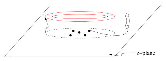
Figure 1: The cycle $\Delta$ formed by a closed loop in the base and a 1-cycle in the fiber.

The homology class of this $T^{3}$ is equal to the sum of the homology classes of 3-cycles $S_{i}$ which are topologically $S^{3}$ [19, 10]. Let us denote by $z_{i}$ the points in the z-plane where the elliptic fibration degenerates. There are $N+3$ such points for the case of the affine $E_{N}$ background. The 3-cycles $S_{i}$ are formed by taking a path connecting $z_{i}$ to $z=0$, the 1-cycle of the elliptic fibration which degenerates at $z_{i}$ and the circle of the $\mbox{C}\!\!\!\mbox{I}^{\,\times}$ fibration. The geometry of the cycle $S_{i}$ is shown in Fig. 2. Thus there are $N+3$ independent 3-cycles in this geometry.

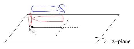
Figure 2: The 3-cycle with topology of $S^{3}$.

The intersection number of these 3-cycles can be calculated easily. From Fig. 2 it is clear that two cycles $S_{i}$ and $S_{j}$ only intersect above the point $z=0$ as long as $z_{i}\neq z_{j}$. Above $z=0$ we have a smooth elliptic fiber and the 3-cycle $S_{i}$ wraps a 1-cycle $C_{i}$ of the this elliptic fiber which degenerates at $z=z_{i}$. If $C_{i}$ and $C_{j}$ have the charge $(p_{i},q_{i})$ and $(p_{j},q_{j})$ then the intersection number, ${}^{\#}(S_{i}\cdot S_{j})$, is given by

$${}^{\#}(S_{i}\cdot S_{j})=^{\#}(C_{i}\cdot C_{j})=\mbox{det}\pmatrix{p_{1}&p_{2}\cr q_{1}&q_{2}}\,.$$ (10)

Each 3-cycle $S_{i}$ is mirror to a coherent sheaf $F_{i}$ on the del Pezzo surface ${\cal B}_{N}$. If $f:{\cal B}_{N}\mapsto Y_{N}$ is the embedding of the del Pezzo surface in Calabi-Yau threefold $Y_{N}$ then we denote by $f_{!}F_{i}$ the coherent sheaf on $Y_{N}$ obtained by extending $F_{i}$ by zero outside ${\cal B}_{N}$ [11]. A bilinear product which counts the number of fermionic zero modes of the string stretched between two sheaves $f_{!}F_{i}$ and $f_{!}F_{j}$ is given by [11]

$$I_{Y_{N}}=\int_{Y_{N}}\mbox{ch}(f_{!}F_{i})^{*}\mbox{ch}(f_{!}F_{j})\mbox{Td}(Y_{N})$$ (11)

This is an antisymmetric product such that

$$I_{Y_{N}}(f_{!}F_{i},f_{!}F_{j})=\chi_{{\cal B}_{N}}(F_{i},F_{j})-\chi_{{\cal B}_{N}}(F_{j},F_{i})=\mbox{det}\pmatrix{r_{1}&r_{2}\cr d_{\Sigma_{1}}&d_{\Sigma_{2}}}\,.$$ (12)

Where $\mbox{ch}(F_{i})=(r_{i},\Sigma_{i},k_{i})$ and $d_{\Sigma_{i}}=-K_{B_{N}}\cdot\Sigma_{i}$.

Since the map between curves (with and without boundary) in the ${\cal E}_{N}$ manifold and bundles on del Pezzos given in [10, 11] was such that

$$r_{i}=q_{i}\,,$$ (13)

$$d_{\Sigma_{i}}=p_{i}\,.$$

We see that

$$I_{Y_{N}}(f_{!}F_{i},f_{!}F_{j})=\mbox{det}\pmatrix{r_{1}&r_{2}\cr d_{\Sigma_{1}}&d_{\Sigma_{2}}}=-\mbox{det}\pmatrix{p_{1}&p_{2}\cr q_{1}&q_{2}}=-^{\#}(S_{i}\cdot S_{j})\,.$$ (14)

Thus the three cycle on which D6-brane is wrapped is given by

$$[T^{3}]=\sum_{i=1}^{k+3}S_{a}\,.$$ (15)

and therefore the gauge group $G$ and the quiver matrix $Q_{ij}$ from which quiver diagrams can be constructed is given by

$$G := \prod_{i=1}^{k+3}U(1)\,,$$ (16)

$$Q_{ij} := I_{Y_{N}}(\pi_{!}F_{i},\pi_{!}F_{j})=-^{\#}(S_{i}\cdot S_{j})\,.$$

3.1 Symmetric adjacency matrix: The case of the conifold

In quiver theories the adjacency matrix need not be antisymmetric. It turns out to be a special feature of toric del Pezzo singularities. For general singularities there is no principle which will restrict the adjacency matrix to be antisymmetric and typically it will have a symmetric as well as an antisymmetric contribution. Quiver theories which are non-chiral like ${\cal N}=2$ supersymmetric theories have an adjacency matrix which is symmetric. Many other examples have this generic feature. In this section we consider such a case, which is relatively simple to calculate using mirror symmetry, and generates a symmetric adjacency matrix.

The mirror of the blown-up conifold is given by [25],

$$(x_{1}+1)(x_{2}+1)-uv=1-e^{-t}\,.$$ (17)

This equation for the mirror manifold can be obtained from the superpotential of the mirror Landau-Ginzburg theory. The superpotential derived from the linear sigma model charges $(1,1,-1,-1)$ is [16]

$$W(x)=x_{0}+x_{1}+x_{2}+e^{-t}\frac{x_{1}x_{2}}{x_{0}}\,,$$ (18)

where $t$ is the complexified Kähler parameter which determines the size of $\mbox{I}\!\mbox{P}^{1}$ in the blownup geometry. The periods in the LG theory are given by

$$\Pi := \int e^{-W(x)}\frac{dx_{0}dx_{1}dx_{2}}{x_{0}x_{1}x_{2}}\,$$ (19)

$$= \int e^{-x_{0}(1+\hat{x}_{1}+\hat{x}_{2}+e^{-t}\hat{x}_{1}\hat{x}_{2})}\frac{dx_{0}d\hat{x}_{1}d\hat{x}_{2}}{x_{0}\hat{x}_{1}\hat{x}_{2}}\,,$$ (20)

where $\hat{x}_{i}=\frac{x_{i}}{x_{0}}$. To be able to integrate over $x_{0}$ we introduce two more variables $u,v$.

$$\Pi = \int e^{-x_{0}(1+\hat{x}_{1}+\hat{x}_{2}+e^{-t}\hat{x}_{1}\hat{x}_{2}-uv)}dudvdx_{0}\frac{d\hat{x}_{1}d\hat{x}_{2}}{\hat{x}_{1}\hat{x}_{2}}\,$$ (21)

$$= \int\delta(1+\hat{x}_{1}+\hat{x}_{2}+e^{-t}\hat{x}_{1}\hat{x}_{2}-uv)dudv\frac{d\hat{x}_{1}d\hat{x}_{2}}{\hat{x}_{1}\hat{x}_{2}}\,.$$ (22)

Thus the LG periods are equal to the periods of the holomorphic 3-form

$$\Omega=\frac{dudvd\hat{x}_{1}d\hat{x}_{2}}{df\hat{x}_{1}\hat{x}_{2}}\,,$$ (23)

where

$$f:=1+\hat{x}_{1}+\hat{x}_{2}+e^{-t}\hat{x}_{1}\hat{x}_{2}-uv=0\,,$$ (24)

is the equation of the mirror manifold. By rescaling the variables we can write this equation as

$$(\hat{x}_{1}+1)(\hat{x}_{2}+1)-uv=1-e^{-t}$$ (25)

To understand the geometry of 3-cycles in this manifold we introduce the variable $z$ such that

$$(x_{1}+1)(x_{2}+1)=z\,,$$ (26)

$$uv+1-e^{-t}=z\,.$$ (27)

The first equation defines a $\mbox{C}\!\!\!\mbox{I}^{\,\times}$ over the $z$-plane which degenerates at $z=0$. The second equation defines another $\mbox{C}\!\!\!\mbox{I}^{\,\times}$ fibration over the $z$-plane which degenerates at $z_{*}:=1-e^{-t}$. As discussed before, these two fibrations can be used to define an $S^{3}$ which shrinks as $t\mapsto 0$. There also exists a second 3-cycle in this geometry which is topologically a $T^{3}$. This cycle is formed by taking a closed loop encircling the points $z=0$ and $z=z_{*}$ together with the circles of the two $\mbox{C}\!\!\!\mbox{I}^{\,\times}$ fibrations. This $T^{3}$ is actually the sum of two $S^{3}$ as shown in Fig. 3 below.

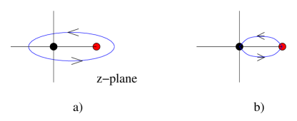
Figure 3: 3-cycles in the mirror of the conifold.

The two $S^{3}$’s intersect each other at two points one above $z=0$ and the other one above $z=z_{*}$. Since the self-intersection number of $[T^{3}]$ is zero there are two hypermultiplets in the representation $(N,\bar{N})$ and $(\bar{N},N)$ in the corresponding gauge theory. The quiver diagram of the gauge theory obtained by wrapping D6-branes on this $T^{3}$ is shown in Fig. 4 below.

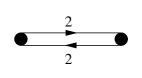
Figure 4: Quiver diagram of the gauge theory on the D3-brane transverse to a conifold singularity.

4 Local toric del Pezzos

The geometry of the local toric del Pezzos is completely determined by the corresponding del Pezzo surface. These Calabi-Yau manifolds are the total space of the anticanonical bundle over the del Pezzo surface. The toric data of these Calabi-Yau manifolds is encoded in the diagrams shown in Fig. 5 below.

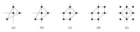
Figure 5: Toric diagrams for the del Pezzo surfaces. a) $\mbox{I}\!\mbox{P}^{2}$, b) $\mbox{I}\!\mbox{P}^{2}$ blown up at one point, c) $\mbox{I}\!\mbox{P}^{2}$ blown up at two points, d) $\mbox{I}\!\mbox{P}^{2}$ blown up at three points, e) $\mbox{I}\!\mbox{P}^{1}\times\mbox{I}\!\mbox{P}^{1}$.

As shown in [21], once the toric data is known it is easy to write down the mirror manifolds,

$$a_{0}+\sum_{\vec{v}\in V}a_{\vec{v}}x_{1}^{v_{1}}x_{2}^{v_{2}}=uv\,.$$ (28)

In the above equation $V$ is the set of vertices of the diagram given in Fig. 5 and $v_{i}$ are the coordinates of the vertex and the variables $x_{i}$ are $\mbox{C}\!\!\!\mbox{I}^{\,\times}$ variables. This equation for the mirror manifold can also be obtained from the superpotential of the mirror Landau-Ginzburg theory following the steps similar to the case of the conifold in the previous section [16, 17].

4.1 Geometry of the mirror manifold

We consider the case of Calabi-Yau obtained from $\mbox{I}\!\mbox{P}^{2}$ blown up at three points. Other local toric del Pezzos can be obtained from this by blowing down exceptional curves. From Fig. 5 it follows that the mirror manifold is given by

$$a_{0}+a_{1}x_{1}+a_{2}x_{2}+\frac{a_{3}}{x_{1}}+\frac{a_{4}}{x_{2}}+a_{5}\frac{x_{1}}{x_{2}}+a_{6}\frac{x_{2}}{x_{1}}=uv\,.$$ (29)

Since $x_{i}$ are $\mbox{C}\!\!\!\mbox{I}^{\,\times}$ variables we can rescale them and simplify the above equation,

$$1+x_{1}+x_{2}+\frac{e^{-t_{1}}}{x_{1}}+\frac{e^{-t_{2}}}{x_{2}}+e^{-t_{3}}\frac{x_{1}}{x_{2}}+e^{-t_{4}}\frac{x_{2}}{x_{1}}=uv\,.$$ (30)

By introducing another complex variable $w$ we can write the above equation as a cubic polynomial in $\mbox{I}\!\mbox{P}^{2}$ and thus representing a genus one curve,

$$z\,x_{1}x_{2}w = x_{1}x_{2}(x_{1}+x_{2}+w)+wx_{2}(e^{-t_{1}}w+e^{-t_{4}}x_{2})+wx_{1}(e^{-t_{2}}w+e^{-t_{3}}x_{1})\,,$$

$$z = uv\,.$$ (31)

The complex structure parameters $a_{i}$ of the mirror manifold are related to the Kähler structure parameters $\{t_{1},t_{2},t_{3},t_{4}\}$ of the original manifold. By redefining coordinates we can write the first equation in the Weierstrass form representing the manifold ${\cal E}_{3}$. The second equation defines a $\mbox{C}\!\!\!\mbox{I}^{\,\times}$ fibration over the complex plane with coordinate $z$. The circle of this fibration degenerates at $z=0$. The first equation defines an elliptic fibration over the $z$-plane. The fibration degenerates at six points on the $z$-plane, $\{z_{*,i}~{}|~{}i=1,\cdots,6\}$. The position of the degenerate fibers depend on the Kähler parameters $\{t_{1},t_{2},t_{3},t_{4}\}$.

As discussed in the previous section. Using these two fibrations we can construct 3-cycles with topology of an $S^{3}$ such that their sum is topologically a $T^{3}$. The matter content of the gauge theory obtained by wrapping D6-branes on this $T^{3}$ is encoded in the intersection matrix of the basis 3-cycles $S_{i}$. In order to calculate the intersection matrix we need the charges of the 1-cycles of the elliptic fibration which degenerate at $z=z_{i}$. These charges are not hard to determine since degenerate fibers of the ${\cal E}_{N}$ are already classified and correspond to the charges of the external legs of the toric diagram of local toric del Pezzos [22]. Thus the intersection number of 3-cycles in the mirror geometry is given by the toric diagram of the original manifold.

The fractional branes in the original geometry are mirror to 3-cycles which can become massless as we change the complex structure of the mirror manifold. The cycles $S_{i}$ that we defined earlier from the basis of such massless 3-cycles and are mirror to the fractional branes. The fractional branes have the RR charge of an exceptional bundle on the del Pezzo surface. This is because on the mirror side $b_{1}(S^{3})=0$, implying that the moduli space of $S^{3}$ is zero dimensional. In [10] the map between bundles on del Pezzo surfaces and 3-cycles in the mirror geometry was given. An important point to keep in mind is the Picard Lefshetz monodromy action on the 3-cycles in the mirror geometry which implies that gauge theories with different matter content can be obtained from the same underlying geometry. This phenomenon was termed “toric duality” in [7]. Different quiver theories coming from the same del Pezzo geometries were listed in that paper with a larger set of examples given in [8]. We will discuss this phenomenon in detail elsewhere [12].

local ${\cal B}_{0}$:

This case has been studied in several papers [26, 27, 28] and can be treated by the usual orbifold methods since it is the resolution of $\mbox{C}\!\!\!\mbox{I}^{\,3}/{\sf Z\!\!\!Z}_{3}$. However, we include this case here for completeness. The charge of the vanishing cycles of the elliptic fibration over the $z$-plane, which is part of the mirror manifold, is determined by the toric diagram of local $\mbox{I}\!\mbox{P}^{2}$, Fig. 6.

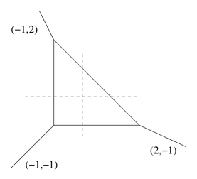
Figure 6: The toric diagram of local $\mbox{I}\!\mbox{P}^{2}$.

This diagram and the diagrams which follow coincide with the $(p,q)$ 5-brane webs of five dimensional field theories [20].

The vanishing 1-cycles which define the 3-cycles in the mirror geometry are

$$C_{1}=(2,-1)\,,\,\,\,\,C_{2}=(-1,2)\,,\,\,\,\,C_{3}=(-1,-1)\,,$$ (32)

and, using equation (10), the intersection matrix of corresponding 3-cycles $S_{i}$ is

$${\cal I}^{0}_{ij}:=^{\#}(S_{i}\cdot S_{j})=^{\#}(C_{i}\cdot C_{j})=\pmatrix{0&3&-3\cr-3&0&3\cr 3&-3&0}\,.$$ (33)

Since there are no mutually local 1-cycles the gauge group is abelian and is just

$$G=\mbox{U}(1)\times\mbox{U}(1)\times\mbox{U}(1)\,.$$ (34)

¿From the above intersection matrix we obtain the quiver diagram of the gauge theory on the D3-branes transverse to the singularity $\mbox{C}\!\!\!\mbox{I}^{\,3}/{\sf Z\!\!\!Z}_{3}$ Fig. 7.

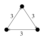
Figure 7: The quiver diagram obtained from the intersection matrix ${\cal I}^{0}_{ij}$. The integer on the line indicates the multiplicity of chiral multiplets.

There are three fractional branes, which we will denote by $F_{1,2,3}$, in this geometry mirror to $S_{1,2,3}$. They are bound states of D7, D5 and D3-branes wrapped on the 4-cycle and various 2-cycles of the del Pezzo. These fractional branes in the large volume limit can be identified with vector bundles on the del Pezzo surface. As shown in the appendix in this geometry they have the following charges ,

$$S_{1}\,:\,\,\mbox{ch}(F_{1}) = (-1,l,-\frac{1}{2})\,,$$ (35)

$$S_{2}\,:\,\,\mbox{ch}(F_{2}) = (2,-l,-\frac{1}{2})\,,$$

$$S_{3}\,\,:\,\,\mbox{ch}(F_{3}) = (-1,0,0)\,.$$

Where $l$ is the generator of $H_{2}(\mbox{I}\!\mbox{P}^{2},{\sf Z\!\!\!Z})$.

local ${\cal B}_{1}$:

In this case we cannot use the usual orbifold techniques directly to determine the quiver. The toric diagram of the local ${\cal B}_{1}$ is shown in Fig. 8 below.

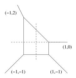
Figure 8: The toric diagram of local ${\cal B}_{1}$.

From the toric diagram it follows that the charges of the vanishing 1-cycles defining the 3-cycles in the mirror geometry are given by

$$C_{1}=(1,-1)\,,\,\,C_{2}=(1,0)\,,\,\,C_{3}=(-1,2)\,,\,\,C_{4}=(-1,-1)\,.$$ (36)

The intersection matrix of the corresponding 3-cycles is given by

$${\cal I}^{1}_{ij}:=^{\#}(S_{i}\cdot S_{j})=^{\#}(C_{i}\cdot C_{j})=\pmatrix{0&1&1&-2\cr-1&0&2&-1\cr-1&-2&0&3\cr 2&1&-3&0}\,.$$ (37)

As in the case of ${\cal B}_{0}$ we see that there are no mutually local 1-cycles and therefore the gauge group, $G$, is given by

$$G=\mbox{U}(1)\times\mbox{U}(1)\times\mbox{U}(1)\times\mbox{U}(1)\,.$$ (38)

The quiver diagram obtained from the above intersection matrix is shown in Fig. 9.

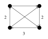
Figure 9: The quiver diagram obtained from the intersection matrix ${\cal I}^{1}_{ij}$.

The fractional branes, denoted by $F_{i}$, in this geometry have the following charges,

$$S_{1}\,:\,\,\mbox{ch}(F_{1}) = (-1,l-E_{1},0)\,,$$ (39)

$$S_{2}\,:\,\,\mbox{ch}(F_{2}) = (0,E_{1},-\frac{1}{2})\,,$$

$$S_{3}\,:\,\,\mbox{ch}(F_{3}) = (2,-l,-\frac{1}{2})\,,$$

$$S_{4}\,:\,\,\mbox{ch}(F_{4}) = (-1,0,0)\,.$$

Where $E_{1}$ is the exceptional curve which together with $l$ forms the basis of $H_{2}({\cal B}_{1})$ such that ${}^{\#}(E_{1}\cdot E_{1})=-1$ and ${}^{\#}(l\cdot E_{1})=0$.

local $F_{0}$:

The toric diagram of local $F_{0}$ is shown in the Fig. 10 below.

Figure 10: The toric diagram of local $\mbox{I}\!\mbox{P}^{1}\times\mbox{I}\!\mbox{P}^{1}$.

For this case the vanishing 1-cycles are

$$C_{1}=(1,-1)\,,\,C_{2}=(1,1)\,,\,C_{3}=(-1,1)\,,\,C_{4}=(-1,-1)\,.$$ (40)

The corresponding intersection matrix is

$$I_{ij}=\pmatrix{0&2&-2&0\cr-2&0&0&2\cr 2&0&0&-2\cr 0&-2&2&0}\,.$$ (41)

And the corresponding quiver diagram is

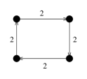
Figure 11: Quiver diagram obtained from ${\cal I}_{ij}$.

The fractional branes have the following charges,

$$S_{1}\,:\,\,\mbox{ch}(F_{1}) = (-1,l_{1},0)\,,$$ (42)

$$S_{2}\,:\,\,\mbox{ch}(F_{2}) = (1,l_{2}-l_{1},-1)\,,$$

$$S_{3}\,:\,\,\mbox{ch}(F_{3}) = (1,-l_{2},0)\,,$$

$$S_{4}\,:\,\,\mbox{ch}(F_{4}) = (-1,0,0)\,.$$

local ${\cal B}_{2}$:

Now consider the case of local ${\cal B}_{2}$. In this case the toric diagram is shown in Fig. 12 below.

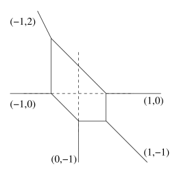
Figure 12: The toric diagram of local $B_{2}$.

The vanishing 1-cycles are

$$C_{1}=(1,-1)\,,\,C_{2}=(1,0)\,,\,C_{3}=(-1,2)\,,\,C_{4}=(-1,0)\,,\,C_{5}=(0,-1)\,.$$ (43)

The intersection matrix of 3-cycles is given by

$${\cal I}^{2}_{ij}:=^{\#}(S_{i}\cdot S_{j})=^{\#}(C_{i}\cdot C_{j})=\pmatrix{0&1&1&-1&-1\cr-1&0&2&0&-1\cr-1&-2&0&2&1\cr 1&0&-2&0&1\cr 1&1&-1&-1&0}\,.$$ (44)

The corresponding quiver diagram is shown in Fig. 13.

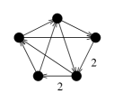
Figure 13: The quiver diagram obtained from ${\cal I}^{2}_{ij}$. The integers on the lines indicate multiplicity.

Since all vanishing 1-cycles are mutually non-local the gauge group, $G$, is

$$G=\mbox{U}(1)\times\mbox{U}(1)\times\mbox{U}(1)\times\mbox{U}(1)\times\mbox{U}(1)\,.$$ (45)

The charges of the fractional branes in this geometry are,

$$S_{1}\,:\,\,\mbox{ch}(F_{1}) = (-1,l-E_{1},0)\,,\,\,$$ (46)

$$S_{2}\,:\,\,\mbox{ch}(F_{2}) = (0,E_{1},-\frac{1}{2})\,,\,\,$$

$$S_{3}\,:\,\,\mbox{ch}(F_{3}) = (2,-l,-\frac{1}{2})\,,$$

$$S_{4}\,:\,\,\mbox{ch}(F_{4}) = (0,-E_{2},-\frac{1}{2})\,,\,\,$$

$$S_{5}\,:\,\,\mbox{ch}(F_{5}) = (-1,E_{2},\frac{1}{2})\,.$$

local ${\cal B}_{3}$:

${\cal B}_{3}$ is the last toric del Pezzo and is given by $\mbox{I}\!\mbox{P}^{2}$ blownup at three points or $\mbox{I}\!\mbox{P}^{1}\times\mbox{I}\!\mbox{P}^{1}$ blownup at two points. The toric diagram is shown in Fig. 14.

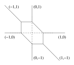
Figure 14: Toric diagram of local $B_{3}$

From the toric diagram we can determine the charge of the vanishing 1-cycles,

$$C_{1} = (1,-1)\,,\,C_{2}=(1,0)\,,\,C_{3}=(0,1)\,,\,$$ (47)

$$C_{4} = (-1,1)\,,\,C_{5}=(-1,0)\,,\,C_{6}=(0,-1)\,.$$

The intersection matrix of corresponding 3-cycles is,

$${\cal I}^{3}_{ij}=\pmatrix{0&1&1&0&-1&-1\cr-1&0&1&1&0&-1\cr-1&-1&0&1&1&0\cr 0&-1&-1&0&1&1\cr 1&0&-1&-1&0&1\cr 1&1&0&-1&-1&0}\,.$$ (48)

The corresponding quiver diagram is shown in Fig. 15 below.

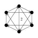
Figure 15: Quiver diagram obtained from ${\cal I}^{3}_{ij}$.

The fractional branes for these cases are

$$S_{1}\,:\,\,\mbox{ch}(F_{1}) = (-1,l-E_{1},0)\,,\,\,$$ (49)

$$S_{2}\,:\,\,\mbox{ch}(F_{2}) = (0,E_{1},-\frac{1}{2})\,,\,\,$$

$$S_{3}\,:\,\,\mbox{ch}(F_{3}) = (1,-E_{3},-\frac{1}{2})$$

$$S_{4}\,:\,\,\mbox{ch}(F_{4}) = (1,-l+E_{3},0)\,,$$

$$S_{5}\,:\,\,\mbox{ch}(F_{5}) = (0,-E_{2},-\frac{1}{2})\,,\,\,$$

$$S_{6}\,:\,\,\mbox{ch}(F_{6}) = (-1,E_{2},\frac{1}{2})\,.$$

Note that in all the cases discussed above the sum of fractional branes is equal to a 0-cycle and is required by mirror symmetry.

5 Non-Toric local del Pezzos

Non-toric del Pezzo surfaces are obtained by blowing up $N$ ($4\leq N\leq 8$) points of $\mbox{I}\!\mbox{P}^{2}$. We will denote, as before, by $E_{i}$ the i-th exceptional curve. It was shown in [22] that diagrams similar to the toric diagram of the previous section can also be drawn for non-toric del Pezzos. The important difference between these and the toric diagrams is that the diagrams for non-toric del Pezzos will have parallel legs. This is simply the fact that in the mirror manifold the elliptic fibration has mutually local vanishing 1-cycles. The elliptic fibration of the mirror manifold in this case are the affine $E_{N}$ ($4\leq N\leq 8$) backgrounds [10]. The charge of the vanishing 1-cycles are known in these cases and therefore we can write down the quiver diagrams and the gauge groups which will have non-abelian factors for such cases.

local ${\cal B}_{4}$:

We consider cases of $\mbox{I}\!\mbox{P}^{2}$ blown up at four points here. The web picture is shown in Fig. 16. The calculation proceeds with no essential difficulties.

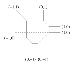
Figure 16: The web diagram of local $B_{4}$.

We have the following basis of 1-cycles for the geometry in Fig. 16.

$$C_{1} = (0,-1)\,,\,C_{2}=C_{3}=(1,0)\,,\,C_{4}=(0,1)\,,$$

$$\,C_{5} = (-1,1)\,,\,C_{6}=(-1,0)\,,\,C_{7}=(0,-1)\,.$$

The gauge group in this case is,

$$G=\prod_{a=1}^{7}\mbox{U}(1)_{a}\,.$$ (50)

The corresponding intersection matrix which determines the quiver diagram is,

$$I_{ij}=C_{i}\cdot C_{j}=\pmatrix{0&1&1&0&-1&-1&0\cr-1&0&0&1&1&0&-1\cr-1&0&0&1&1&0&-1\cr 0&-1&-1&0&1&1&0\cr 1&-1&-1&-1&0&1&1\cr 1&0&0&-1&-1&0&1\cr 0&1&1&0&-1&-1&0}\,.$$ (51)

The above intersection matrix gives the quiver diagram shown in Fig. 17 below.

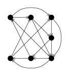
Figure 17: Quiver diagram obtained from the above intersection matrix $I_{ij}$.

The fractional branes for this case are

$$S_{1}\,:\,\,\mbox{ch}(F_{1}) = (-1,l-E_{1}-E_{4},\frac{1}{2})$$ (52)

$$S_{2}\,:\,\,\mbox{ch}(F_{2}) = (0,E_{4},-\frac{1}{2})\,,\,\,$$

$$S_{3}\,:\,\,\mbox{ch}(F_{3}) = (0,E_{1},-\frac{1}{2})\,,\,\,$$

$$S_{4}\,:\,\,\mbox{ch}(F_{4}) = (1,-E_{3},-\frac{1}{2})$$

$$S_{5}\,:\,\,\mbox{ch}(F_{5}) = (1,-l+E_{3},0)$$

$$S_{6}\,:\,\,\mbox{ch}(F_{6}) = (0,-E_{2},-\frac{1}{2})\,,\,\,$$

$$S_{7}\,:\,\,\mbox{ch}(F_{7}) = (-1,E_{2},\frac{1}{2})\,.$$

local ${\cal B}_{5}$

The web picture for this case is shown in Fig. 18 below.

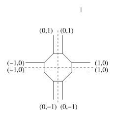
Figure 18: The web diagram of local $B_{5}$.

From Fig. 18 we have the following 1-cycles,

$$C_{1} = (0,-1)\,,\,C_{2}=C_{3}=(1,0)\,,\,C_{4}=C_{5}=(0,1)\,,\,C_{6}=C_{7}=(-1,0)\,,\,C_{8}=(0,-1)\,.$$

The gauge group, $G$, is given by

$$G=\prod_{a=1}^{8}\mbox{U}(1)_{a}\,.$$ (53)

The quiver diagram corresponding to the intersection matrix is shown in Fig. 19.

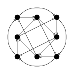
Figure 19: Quiver diagram obtained from the intersection matrix of $C_{i}$’s.

The charge of the fractional branes is given by

$$S^{a}_{1}\,:\,\,\mbox{ch}(F^{a}_{1}) = (-1,l-E_{1}-E_{4},\frac{1}{2})$$ (54)

$$S^{a}_{2}\,:\,\,\mbox{ch}(F^{a}_{2}) = (0,E_{4},-\frac{1}{2})\,,\,\,$$

$$S^{a}_{3}\,:\,\,\mbox{ch}(F^{a}_{3}) = (0,E_{1},-\frac{1}{2})\,,\,\,$$

$$S^{a}_{4}\,:\,\,\mbox{ch}(F^{a}_{4}) = (1,-E_{3},-\frac{1}{2})$$

$$S^{a}_{5}\,:\,\,\mbox{ch}(F^{a}_{5}) = (1,-E_{5},-\frac{1}{2})$$

$$S^{a}_{6}\,:\,\,\mbox{ch}(F^{a}_{6}) = (0,-l+E_{3}+E_{5},\frac{1}{2})$$

$$S^{a}_{7}\,:\,\,\mbox{ch}(F^{a}_{7}) = (0,-E_{2},-\frac{1}{2})\,,\,\,$$

$$S^{a}_{8}\,:\,\,\mbox{ch}(F^{a}_{8}) = (-1,E_{2},\frac{1}{2})\,.$$

local ${\cal B}_{6}$

The web picture for this case is shown in Fig. 20 below. For this case and later ones we will only give the charge of the 1-cycles from which the intersection matrix and the quiver diagram can be obtained easily.

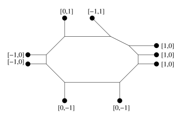
Figure 20: The web diagram of local $B_{6}$.

The 1-cycles are

$$C_{1} = (0,-1)\,,\,C_{2}=C_{3}=C_{4}=(1,0)\,,\,C_{5}=(-1,1)\,,\,C_{6}=(0,1)\,,\,$$ (55)

$$C_{7} = C_{8}=(-1,0)\,,\,C_{9}=(0,-1)\,.$$

The gauge group, $G$, in this case is,

$$G=\prod_{a=1}^{9}\mbox{U}(1)_{a}\,.$$ (56)

The fractional brane charges for this geometry are given below,

$$S_{1}\,:\,\,\mbox{ch}(F_{1}) = (-1,l-E_{1}-E_{4},\frac{1}{2})$$ (57)

$$S_{2}\,:\,\,\mbox{ch}(F_{2}) = (0,E_{4},-\frac{1}{2})\,,\,\,$$

$$S_{3}\,:\,\,\mbox{ch}(F_{3}) = (0,E_{1},-\frac{1}{2})\,,\,\,$$

$$S_{4}\,:\,\,\mbox{ch}(F_{4}) = (0,l-E_{3}-E_{6},-\frac{1}{2})$$

$$S_{5}\,:\,\,\mbox{ch}(F_{5}) = (1,-l+E_{6},0)$$

$$S_{6}\,:\,\,\mbox{ch}(F_{6}) = (1,-E_{5},-\frac{1}{2})$$

$$S_{7}\,:\,\,\mbox{ch}(F_{7}) = (0,-l+E_{3}+E_{5},\frac{1}{2})$$

$$S_{8}\,:\,\,\mbox{ch}(F_{8}) = (0,-E_{2},-\frac{1}{2})\,,\,\,$$

$$S_{9}\,:\,\,\mbox{ch}(F_{9}) = (-1,E_{2},\frac{1}{2})\,.$$

local ${\cal B}_{7}$

The web diagram is shown in Fig. 21 below.

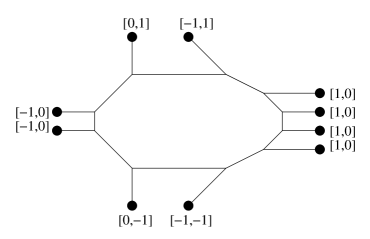
Figure 21: The web diagram of local $B_{7}$.

The 1-cycles follow from the web diagram

$$C_{1} = (-1,-1)\,,\,C_{2}=C_{3}=C_{4}=C_{5}=(1,0)\,,\,C_{6}=(-1,1)\,,\,$$ (58)

$$C_{7} = (0,1)\,,\,C_{8}=C_{9}=(-1,0)\,,\,C_{10}=(0,-1)\,.$$

The gauge group in this case is,

$$G=\prod_{a=1}^{10}\mbox{U}(1)_{a}\,.$$ (59)

The fractional brane charges are,

$$S_{1}\,:\,\,\mbox{ch}(F_{1}) = (-1,l-E_{1}-E_{4}-E_{7},1)$$ (60)

$$S_{2}\,:\,\,\mbox{ch}(F_{2}) = (0,E_{7},-\frac{1}{2})$$

$$S_{3}\,:\,\,\mbox{ch}(F_{3}) = (0,E_{4},-\frac{1}{2})\,,\,\,$$

$$S_{4}\,:\,\,\mbox{ch}(F_{4}) = (0,E_{1},-\frac{1}{2})\,,\,\,$$

$$S_{5}\,:\,\,\mbox{ch}(F_{5}) = (0,l-E_{3}-E_{6},-\frac{1}{2})\,,\,$$

$$S_{6}\,:\,\,\mbox{ch}(F_{6}) = (1,-l+E_{6},0)$$

$$S_{7}\,:\,\,\mbox{ch}(F_{7}) = (1,-E_{5},-\frac{1}{2})$$

$$S_{8}\,:\,\,\mbox{ch}(F_{8}) = (0,-l+E_{3}+E_{5},\frac{1}{2})$$

$$S_{9}\,:\,\,\mbox{ch}(F_{9}) = (0,-E_{2},-\frac{1}{2})$$

$$S_{10}\,:\,\,\mbox{ch}(F_{10}) = (-1,E_{2},\frac{1}{2})\,,\,\,$$

local ${\cal B}_{8}$

This is the last del Pezzo surface and the corresponding web diagram is shown in Fig. 22.

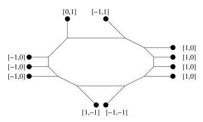
Figure 22: The web diagram of local $B_{8}$.

The vanishing 1-cycles are,

$$C_{1} = (-1,-1)\,,\,C_{2}=C_{3}=C_{4}=C_{5}=(1,0)\,,\,C_{6}=(-1,1)\,,\,$$ (61)

$$C_{7} = (0,1)\,,\,C_{8}=C_{9}=C_{10}=(-1,0)\,,\,C_{11}=(1,-1)\,.$$

The gauge group is given by,

$$G=\prod_{a=1}^{11}\mbox{U}(1)_{a}\,.$$ (62)

The corresponding fractional brane charges are,

$$S_{1}\,:\,\,\mbox{ch}(F_{1}) = (-1,l-E_{1}-E_{4}-E_{7},1)$$ (63)

$$S_{2}\,:\,\,\mbox{ch}(F_{2}) = (0,E_{7},-\frac{1}{2})\,,\,\,$$

$$S_{3}\,:\,\,\mbox{ch}(F_{3}) = (0,E_{4},-\frac{1}{2})\,,\,\,$$

$$S_{4}\,:\,\,\mbox{ch}(F_{4}) = (0,E_{1},-\frac{1}{2})\,,\,\,$$

$$S_{5}\,:\,\,\mbox{ch}(F_{5}) = (0,l-E_{3}-E_{6},-\frac{1}{2})$$

$$S_{6}\,:\,\,\mbox{ch}(F_{6}) = (1,-l+E_{6},0)$$

$$S_{7}\,:\,\,\mbox{ch}(F_{7}) = (1,-E_{5},-\frac{1}{2})$$

$$S_{8}\,:\,\,\mbox{ch}(F_{8}) = (0,-l+E_{3}+E_{5},\frac{1}{2})$$

$$S_{9}\,:\,\,\mbox{ch}(F_{9}) = (0,-E_{2},-\frac{1}{2})\,,\,\,$$

$$S_{10}\,:\,\,\mbox{ch}(F_{10}) = (0,-E_{8},-\frac{1}{2})\,\,$$

$$S_{11}\,:\,\,\mbox{ch}(F_{11}) = (-1,E_{2}+E_{8},1)\,.$$

Note that in all the cases we discussed the sum of fractional branes is equal to a 0-cycle as required by mirror symmetry,

$$\sum_{i=1}^{N+3}\mbox{ch}(F_{i})=(0,0,-1)\,.$$ (64)

Also it is easy to check that the set $\{F_{1},\cdots,F_{N+3}\}$, for $0\leq N\leq 8$, is an exceptional collection forming a helix on ${\cal B}_{N}$. Another interesting point to note is that since

$${}^{\#}(S_{i}\cdot\sum_{j=1}^{N+3}S_{j})=0\,,$$ (65)

therefore it follows that in corresponding quiver diagram, for each node, the number of incoming arrows is equal to the number of outgoing arrows. This statement in terms of gauge theory just states that there are no chiral anomalies for each of the gauge group factors involved.

Appendix A Fractional Brane Charges

In this appendix we explain the calculation of fractional brane charges. This calculation uses the map the between 3-cycle in the mirror geometry and vector bundles on del Pezzo surfaces studied in [10, 11].

Recall that the geometry we are considering is an elliptic and a $\mbox{C}\!\!\!\mbox{I}^{\,\times}$ fibration over the z-plane. The $\mbox{C}\!\!\!\mbox{I}^{\,\times}$ fibration is universal in the sense that for all cases it degenerates at $z=0$. Thus all the information is contained in the elliptic fibration over the z-plane and we can map all the 3-cycles in this geometry to string junctions with support on 7-branes and a D3-brane. The $(p,q)$ 7-branes correspond to the degenerate fibers of the elliptic fibration and the D3-brane corresponds to the degeneration of the $\mbox{C}\!\!\!\mbox{I}^{\,\times}$ fibration. Thus BPS states of the ${\cal N}=2$ theory obtained from compactification of Type IIB on the mirror manifold are the same as the BPS states of the $N=2$ theory on the D3-brane in the background of certain mutually non-local 7-branes. The 7-brane backgrounds which correspond to the mirror of local del Pezzo surfaces were studied in detail in [19] and lead to broken affine $E_{N}$ gauge symmetry on the 7-branes.

$${\cal E}_{N}\,:\,\,\underbrace{[1,0]\cdots[1,0]}_{N}\,[2,-1]\,[-1,2]\,[-1,-1]$$ (66)

Here the numbers in square brackets denote the $(p,q)$ charges of the corresponding 7 branes. The only information we need concerning the map is that if a string junction $J$ ends on the D3-brane with charge $(p,q)$ then the rank $r$ and the degree of the first Chern class $d_{c_{1}}$ are given by

$$r = q\,,$$ (67)

$$d_{c_{1}} = p-q\,.$$

Also the self-intersection number of the junction is equal $-\chi(V,V)$,

$$-J\cdot J=\chi(V,V):=\int_{X}\mbox{ch}(V\otimes V^{*})\mbox{Td}(X)=r^{2}-c_{1}\cdot c_{1}+2rk,$$ (68)

where $k=\int_{X}\mbox{ch}_{2}(V)$. Eq(A) and Eq(68) imply that string junctions with support only on a single [1,0] 7-brane corresponds to the bundle (sheaf)

$$\mbox{ch}(V_{a})=(0,E_{a},-\frac{1}{2})\,,\,\,\,a=1,\cdots,n$$ (69)

The bundles corresponding to other string junctions living on $[2,-1]$ , $[-1,2]$ and $[-1,-1]$ can also be obtained using Eq(A) and Eq(68). Consider the case of string junction on $[n,m]$ 7-brane. From Eq(A) it follows that the corresponding bundle has $ch_{0}=m$. Since $dimH_{2}(B_{0})=1$ with generator $l$ the first Chern class of the bundle is a multiple of $l$. From $d_{c_{1}}=p-q$ it follows that $c_{1}=\frac{n-m}{3}l$. The Self-intersection number of the junction is (since it is a half-sphere) $-1$ and therefore Eq(68) implies that $ch_{2}=\frac{n^{2}-2nm-8m^{2}+9}{18m}$. Thus we the following map

$$[n,m]\,\, : \,\mbox{ch}(V)=(m,\frac{n-m}{3}l,\frac{n^{2}-2nm-8m^{2}+9}{18m})\,,$$ (70)

$$[2,-1]\,\, : \,\mbox{ch}(V)=(-1,l,-\frac{1}{2})\,,$$

$$[-1,2]\,\, : \,\mbox{ch}(V)=(2,-l,-\frac{1}{2})\,,$$

$$[-1,-1]\,\, : \,\mbox{ch}(V)=(-1,0,0)\,.$$

Since all other junctions can be formed by linear combination of these basic string junctions Eq(69) and Eq(A) provide the complete map.

local ${\bf{\cal B}_{1}}$: As an example we work out the charges of fractional branes for local ${\cal B}_{1}$.

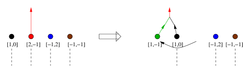
Figure 23: The branch cut move and the corresponding action on the string junction.

The branch cut moves which takes us from the configuration given in equation (66) to the one obtained from the toric diagram is shown in Fig. 23. The sum of junctions on [1,-1] and [1,0] is the same as the junction on [2,-1], as shown in Fig. 23, therefore

$$\mbox{ch}(F_{[1,-1]}) = \mbox{ch}(F_{[2,-1]})-\mbox{ch}(F_{[1,0]})$$

$$= (-1,l,-\frac{1}{2})-(0,E_{1},-\frac{1}{2})$$

$$= (-1,l-E_{1},0)$$

Similarly we determine the charge of fractional branes in other local del Pezzo geometries by starting with the configuration given in (66) and converting in into the one given by the toric diagram using branch cut moves.

References

- [1] S. Katz, A. Klemm, C. Vafa, “Geometric Engineering of Quantum Field Theories,” Nucl. Phys B497 (1997) 173-195, hep-th/9609239.
- [2] S. Katz, P. Mayr, C, Vafa, “Mirror Symmetry and Exact Solution of N=2 Theories 4D N=2 Gauge Theories I”, Adv. Theor. Math. Phys. 1 (1998) 53-114, hep-th/9706110.
-
[3]
F. Cachazo, K. Intriligator, C. Vafa, “A Large N Duality via a
Geometric Transition,” Nucl. Phys. B603 (2001) 2-41,
hep-th/0103067,
F. Cachazo, S. Katz, C. Vafa, “Geometric Transitions and N=1 Quiver Theories,” hep-th/0108120. - [4] D.R. Morrison, N. Seiberg, “Extremal Transitions and Five-Dimensional Supersymmetric Field Theories,” Nucl. Phys. B483 (1997) 229-247, hep-th/9609070.
- [5] M. R. Douglas, S. Katz, C. Vafa, “Small Instantons, del Pezzo Surfaces and Type I′ Theory,” Nucl. Phys. B497 (1997) 155-172, hep-th/9609071.
- [6] K. Intriligator, D.R. Morrison, N. Seiberg, “Five Dimensional Supersymmetric Gauge Theories and Degeneration of calabi-Yau Spaces,” Nucl.Phys. B497 (1997) 56-100, hep-th/9702198.
- [7] B. Feng, A. Hanany, Y. -H. He, “D-Brane Gauge Theories from Toric Singularities and Toric Duality,” hep-th/0003085.
- [8] B. Feng, A. Hanany, Y. -H. He, “Phase Structure of D-brane Gauge Theories and Toric Duality,” hep-th/0104259.
- [9] C. Beasley, B. R. Greene, C. I. Lazaroiu, M.R. Plesser, “D3-branes on partial resolution of abelian quotient singularities of Calabi-Yau threefolds,” Nucl.Phys. B566 (2000) 599-640, hep-th/9907186.
- [10] T. Hauer, A. Iqbal, “Del Pezzo Surfaces and Affine 7-brane Backgrounds,” JHEP 0001 (2000) 043, hep-th/9910054.
- [11] K. Mohri, Y. Onjo, S. K. Yang, “Duality Between String Junctions and D-Branes on Del Pezzo Surfaces,” hep-th/0007243.
- [12] A. Hanany, A. Iqbal, in progress.
-
[13]
S. Katz, C. Vafa, “Geometric Engineering of N=1 Quantum Field
Theories,” Nucl. Phys. B497 (1997) 196-204, hep-th/9611090,
M. Bershadsky, A. Johansen, T. Pantev, V. Sadov, C. Vafa, “F-Theory, geometric Engineering and N=1 Dualities,” Nucl. Phys. B505 (1997) 153-164, hep-th/9612052,
B. Zwiebach, C. Vafa, “N=1 Dualities of SO and USp Gauge Theories and T-Duality of String Theory,” Nucl. Phys. B506 (1997) 143-156, hep-th/9701015,
J. D. Edelstein, K. Oh, R. Tatar, “Orientifold, Geometric Transition and Large N Duality for SO/Sp Gauge Theories,” JHEP 0105 (2001) 009, hep-th/0104037. - [14] D. Berenstein, R. G. Leigh, “Resolution of Stringy Singularities by Non-commutative Algebras”, JHEP 0106 (2001) 030, hep-th/0105229.
- [15] Y. Yamada, S. K. Yang, “Affine 7-brane Backgrounds and Five-Dimensional Theories on ,” Nucl. Phys. B566 (2000) 642-660, hep-th/9907134.
- [16] K. Hori, C. Vafa, “Mirror symmetry,” hep-th/0002002.
- [17] K. Hori, A. Iqbal, C. Vafa, “D-Branes and Mirror Symmetry,” hep-th/0005247.
- [18] A. Sen, B. Zwiebach, “Stable Non-BPS States in F-theory,” hep-th/9907164.
- [19] O. DeWolfe, T. Hauer, A. Iqbal, B. Zwiebach, “Uncovering Infinite Symmetries on [p,q] 7-branes: Kac-Moody Algebras and Beyond,” Adv. Theor. Math. Phys. 3 (1999) 1835-1891, hep-th/9812209.
- [20] O. Aharony, A. Hanany, B. Kol, “Webs of 5-branes, Five dimensional Field Theories and Grid Diagrams,” hep-th/9710116.
- [21] N. C. Leung, C. Vafa, “Branes and Toric Geometry,” Adv. Theor. Math. Phys. 2 (1998) 91-118, hep-th/9711013.
- [22] O. DeWolfe, A. Hanany, A. Iqbal, E. Katz, “Five-branes, Seven-branes and Five-dimensional field Theories,” hep-th/9902179.
- [23] O. DeWolfe, “Affine Lie Algebras, String Junctions and 7-Branes,” Nucl.Phys. B550 (1999) 622-637, hep-th/9809026.
- [24] T. hauer, A. Iqbal, B. Zwiebach, “Duality and Weyl Symmetry of 7-brane Configurations,” hep-th/0002127.
- [25] C. Vafa, “Superstrings and Topological Strings at Large N,” hep-th/0008142.
- [26] D. -E. Diaconescu, J. Gomis, “Fractional Branes and Boundary States in Orbifold Theories,” JHEP 0010 (2000) 001, hep-th/9906242.
- [27] M. R. Douglas, B. Fiol, C. Romelsberger, “The spectrum of BPS branes on a noncompact Calabi-Yau,” hep-th/0003263.
- [28] K. Mohri, Y. Onjo, S.-K. Yang, “Closed Sub-Monodromy Problems, Local Mirror Symmetry and Branes on Orbifolds,” hep-th/0009072.