Quantization of the massless minimally coupled scalar field and the dS/CFT correspondence

Abstract

We consider the quantization of the massless minimally coupled scalar field in de Sitter spacetime. The no-boundary Euclidean prescription naturally picks out the de Sitter invariant vacuum state of Kirsten and Garriga. We extend the dS/CFT correspondence to this case which allows us to interpret the massless field in terms of a Euclidean CFT. The extension is non-trivial and requires careful treatment of the zero mode.

I Introduction

De Sitter spacetime is one of the simplest and most interesting spacetimes allowed by general relativity. If current indications from supernovae, cosmic microwave background and other astronomical data have been interpreted correctly, it seems that the Universe we live in will in fact be asymptotically de Sitter in the infinite future. De Sitter spacetime also plays a central role in the theory of inflation, where an approximately de Sitter spacetime, with exponential expansion, is employed to solve the cosmological flatness and horizon puzzles.

The quantum mechanics of de Sitter spacetime, and matter fields within it, is also of considerable interest. During inflation, massless quantum fields acquire fluctuations on macroscopically large scales, leading to an attractive theory of the origin of structure in the Universe. Indeed this setup provides one of the very few direct observational probes of quantum gravity, since the gravitational waves generated during such a period of early inflation may be directly observable today through the polarization signature they produce on the cosmic microwave sky.

In this article we consider the quantization of the massless minimally coupled scalar field in de Sitter spacetime and its relation to a conformal field living at the boundary. The massless case must be treated separately from the massive case due to the presence of the symmetry $\phi\rightarrow\phi+q$ where $q$ is a space-time constant. This symmetry is relevant for a massless minimally coupled scalar field on any spacetime with compact spatial sections, whereas for spacetimes (such as Minkowski spacetime) with infinite spatial sections, super-selection rules render the symmetry innocuous. As shown by Allen and Folacci [1] the presence of the zero mode implies there is no de Sitter invariant Fock vacuum for the massless field. Nevertheless there is still a de Sitter invariant vacuum as shown by Kirsten and Garriga [8]. We will show that it is this latter vacuum state that is naturally picked out by the no boundary Euclidean prescription.

Recently Strominger [3] has given arguments showing that a scalar field of mass $0<m^{2}<(\frac{d}{2}H)^{2}$ in $dS^{d+1}$ can be related to a conformal field theory living on an $S^{d}$ which may be identified as the boundary (timelike infinity) of de Sitter spacetime[10]. This proposal was formulated in analogy with the AdS/CFT correspondence and arguments suggesting its existence were given in [2, 4]. Using this correspondence it is possible to obtain information about Euclidean conformal field theories from quantum gravity in de Sitter spacetime[5]. It is significant that it does not seems possible to formulate a unitary CFT for the massive fields $m^{2}\geq(\frac{d}{2}H)^{2}$, suggesting that such fields may not arise in a consistent de Sitter quantum gravity. We will extend Strominger’s analysis to the massless case and show that such fields do have a unitary CFT interpretation.

II De Sitter space and the representation theory

The scalar representations of the de Sitter group $SO(1,d+1)$ split into three series[14, 9], the principal series $m^{2}\geq(\frac{d}{2}H)^{2}$, the complementary series $0<m^{2}<(\frac{d}{2}H)^{2}$ and the discrete series whose only physical interesting case is $m^{2}=0$. Under a Wigner-Inönü contraction to the Poincare group only the principal series representations contract to Poincare representations and have an interpretation as particles in the limit of zero cosmological constant[9]. Strominger [3] has shown that complementary series representations have a dual interpretation in terms of a unitary CFT while the principal series representations require a non-unitary description. However, as yet the special case $m^{2}=0$ has not been treated. In the following we shall concentrate on 4 dimensional de Sitter spacetime although everything can easily be generalized to arbitrary dimensions. It is important to consider the de Sitter invariant vacuum in order to obtain information about the conformally invariant vacuum of the dual CFT, and since its structure is subtle we shall consider in detail the role of de Sitter invariance.

The choice of vacuum for a massive scalar field in an arbitrary spacetime is determined by the choice of complex structure [13]. This provides a decomposition of the space of real solutions $\mathcal{S}$ to the equation of motion $[-\nabla^{2}+m^{2}]\phi=0$ into two complex subspaces $\mathcal{S}=\mathcal{V}^{+}\oplus\mathcal{V}^{-}$ such that $\mathcal{V}^{+}/\mathcal{V}^{-}$ has positive/negative Klein-Gordon norm respectively. $\mathcal{V}^{+}$ is then taken to be the single-particle Hilbert space $\mathcal{H}$ and the Hilbert space of the full theory is then taken to be the usual Fock space $\mathcal{F}=\mathcal{C}\oplus\mathcal{H}\oplus\mathcal{H}\otimes\mathcal{H}\oplus\dots$. Demanding that the complex structure (and hence the vacuum) be de Sitter invariant picks out a one-parameter family of inequivalent de Sitter invariant vacua. Requiring that the short distance behaviour of the Hadamard function should be of the same type as that in flat spacetime then uniquely fixes the vacuum. This is known as the Bunch-Davies or Euclidean vacuum[12]. In the massless case the Klein-Gordon inner product and equation of motion are invariant under the symmetry $\phi\rightarrow\phi+q$. Allen and Folacci [1] have shown that this implies that there is no de Sitter invariant complex structure and hence Fock space/vacuum. The situation is analogous to QED and the resolution is to define a vacuum similar to the Gupta-Bleuler vacuum in QED[9] for which de Sitter invariance is recovered. Consequently we need to look for a single-particle Hilbert space defined as a space of positive norm solutions of the equations of motion modulo symmetry transformations.

4d de Sitter spacetime is topologically $R\times S^{3}$ and can be covered with the metric

$$ds^{2}=H^{-2}[-d\tau^{2}+\cosh^{2}\tau(d\chi^{2}+\sin^{2}\chi(d\theta^{2}+\sin^{2}\theta d\phi^{2}))]$$ (1)

with $-\infty<\tau<\infty$, $0\leq\chi,\theta\leq\pi$, $0\leq\phi\leq 2\pi$. These co-ordinates are known as the closed slicing as they provide a foliation in terms of compact $S^{3}$ hypersurfaces. An arbitrary solution of the equations of motion can then be written as a superposition over $S^{3}$ eigenmodes. Thus we are lead naturally to the decomposition $\phi=\phi_{g}+\phi_{z}+\phi^{+}+\phi^{-}$

$$\phi_{g}=const.$$ (2)

$$\phi_{z}=Ha_{z}(2\tan^{-1}\tanh(\tau/2)+\tanh\tau\>{\rm sech}\tau)$$ (3)

$$\phi^{+}=\Sigma_{L>0,lm}a_{Llm}\chi_{L}(\tau)Y_{Llm}(\chi,\theta,\phi)$$ (4)

$$\phi^{-}=\Sigma_{L>0,lm}a^{*}_{Llm}\chi^{*}_{L}(\tau)Y^{*}_{Llm}(\chi,\theta,\phi)$$ (5)

The $Y_{Llm}(\chi,\theta,\phi)$ are the usual spherical harmonics defined on a 3-sphere. The $\chi_{L}(\tau)$ are defined by the massless limit of the usual Bunch-Davies modes[12]

$$\chi_{L}(\tau)=\frac{H}{2}A_{L}[L(\cosh\tau)^{L+2}(1+i\sinh\tau)^{-L-2}+(L+2)(\cosh\tau)^{L}(1+i\sinh\tau)^{-L})]$$ (6)

with $A_{L}=[2(L+2)(L+1)L]^{-1/2}$. Note that they satisfy the reflection symmetry $\chi_{L}(\tau)^{*}=\chi_{L}(-\tau)$. We will denote the subspaces of solutions by $\phi^{+}\in\mathcal{V}^{+}$, $\phi^{-}\in\mathcal{V}^{-}$, $\phi_{g}\in\mathcal{N}$, $\phi_{z}\in\mathcal{Z}$ so that the full space of solutions is given by $\mathcal{S}=\mathcal{V}^{+}\oplus\mathcal{V}^{-}\oplus\mathcal{N}\oplus\mathcal{Z}$. The massless minimally coupled scalar field in de Sitter spacetime belongs to the so-called discrete series representation of the de Sitter group $SO(1,4)$ [14]. A candidate Hilbert space must have positive norm and be closed under the action of the de Sitter group $T(g):\mathcal{H}\rightarrow\mathcal{H}$. In addition the chosen norm must be invariant, $\langle T(g)f,T(g)h\rangle=\langle f,h\rangle$. The natural inner product is the Klein-Gordon inner product (see appendix). Under the action of an arbitrary element of the de Sitter group $g$ the subspaces $\mathcal{V}^{+}$, $\mathcal{V}^{-}$, $\mathcal{N}$, $\mathcal{Z}$ transform as[9]

$$T(g):{\mathcal{N}}\rightarrow{\mathcal{N}}$$ (7)

$$T(g):{\mathcal{Z}}\rightarrow{\mathcal{Z}}\oplus{\mathcal{V^{+}}}\oplus{\mathcal{V^{-}}}\oplus{\mathcal{N}}$$ (8)

$$T(g):{\mathcal{V^{+}}}\rightarrow{\mathcal{V^{+}}}\oplus{\mathcal{N}}$$ (9)

$$T(g):{\mathcal{V^{-}}}\rightarrow{\mathcal{V^{-}}}\oplus{\mathcal{N}}$$ (10)

$T(g)$ denotes the representation of the group element $g$ acting on the space of solutions. To illustrate this we may construct the $SO(1,4)$ generators with the help of the embedding co-ordinates as

$$M_{AB}=i[x_{A}\frac{\partial}{\partial x^{B}}-x_{B}\frac{\partial}{\partial x^{A}}]$$ (12)

Then if we construct the following operator invariant under the $SO(4)$ subgroup (see appendix)

$$\hat{Z}=i\frac{x^{i}}{\sqrt{x_{i}x^{i}}}M_{0i}=\frac{\partial}{\partial\tau}$$ (13)

This operator represents the part of the generators that generates time translations alone, it is only this part that mixes states of different $L$. One observes that

$$\hat{Z}\chi_{1}(\tau)=-\frac{i\sqrt{3}H}{8}-\frac{3i}{2}\chi_{2}(\tau)$$ (14)

$$\hat{Z}\phi_{z}(\tau)=a_{z}\sqrt{3}(\chi_{1}(\tau)+\chi_{1}(\tau)^{*})$$ (15)

with the structure of the higher $L$ terms being always of the form $\hat{Z}\chi_{L}(\tau)=a_{L}\chi_{L+1}(\tau)+b_{L}\chi_{L-1}(\tau)$. It follows that the de Sitter invariant spaces are ${\mathcal{V^{+}}}/{\mathcal{N}}$ and ${\mathcal{V^{-}}}/{\mathcal{N}}$. Since the modes $\phi^{+}$ have positive norm then the Hilbert space that forms the discrete series representation of the de Sitter group is $\mathcal{H}={\mathcal{V^{+}}}/{\mathcal{N}}$. Note that the zero mode $\phi_{z}\in\mathcal{Z}$ does not contribute to the physical state space since if it was included modes of positive norm would be transformed into modes of negative norm violating unitarity. In particular this means that only the $L>0$ modes will contribute to any physical quantity.

III Covariant quantization

Covariant quantization begins with the fundamental quantization condition

$$[\phi(x),\phi(x^{\prime})]=\Delta(x,x^{\prime})$$ (17)

where the commutator function $\Delta(x,x^{\prime})$ is equal to $i$ times the advanced minus retarded Green functions. This incorporates causality from the start and ensures that the commutator of two fields vanishes at spacelike separations. This is distinct from the canonical approach where causality is not immediately apparent and depends on which modes are included. Note that $\Delta(x,x^{\prime})$ is independent of the choice of vacuum state: that information is contained in the Hadamard function we shall consider later.

In the context of de Sitter spacetime $\Delta(x,x^{\prime})$ has a smooth limit as the mass $m$ of the field is taken to zero. So it may be defined as the massless limit of the massive commutator

$$\Delta(x,x^{\prime})=\epsilon(x,x^{\prime})\frac{H^{2}}{8\pi^{2}}(\frac{1}{1-z+i\epsilon}-\ln|1-z+i\epsilon|-\frac{1}{1-z-i\epsilon}+\ln|1-z-i\epsilon|)$$ (18)

$$=-2\pi i\epsilon(x,x^{\prime})\frac{H^{2}}{8\pi^{2}}(\delta(1-z)+\theta(z-1))$$ (19)

where $z(x,x^{\prime})$ is defined in the Appendix. We can then examine the properties of $\Delta(x,x^{\prime})$ in the closed coordinate system, by expanding it in terms of modes on a 3-sphere. Since $\Delta(x,x^{\prime})$ is by definition a solution of the equations of motion it must be a superposition of usual closed slicing modes. In particular this includes the normalizable zero mode. The result can be most usefully written in the form

$$[\phi(x),\phi(x^{\prime})]=i\frac{H^{2}}{4\pi^{2}}(f(\tau^{\prime})-f(\tau))+W^{+}_{n}(x,x^{\prime})-W^{+}_{n}(x^{\prime},x)$$ (20)

where $f(\tau)=2\tan^{-1}\tanh(\tau/2)+{\rm\tanh}\tau\>{\rm sech}\tau$ and can be recognized as the $L=0$ mode term $\phi_{z}$. Here $W^{+}_{n}(x,x^{\prime})$ is the Wightman function constructed out of only the $L>0$ modes

$$W^{+}_{n}(x,x^{\prime})=\Sigma_{L>0lm}\phi_{Llm}(x)\phi^{*}_{Llm}(x^{\prime})$$ (21)

$$=\frac{H^{2}}{8\pi^{2}}[\frac{1}{1-z}-\ln|1-z|-g(\tau)-g(\tau^{\prime})+i(f(\tau)-f(\tau^{\prime}))]+\frac{1}{2}\Delta(x,x^{\prime})$$ (22)

where $g(\tau)={\rm sech}^{2}\tau+\ln(2{\rm sech}\tau)$. The expression for the field $\phi(x)$ which gives rise to these commutation relations is

$$\phi(x)=\frac{H}{2\pi}Q+\frac{H}{2\pi}f(\tau)P+\phi^{+}(x)+\phi^{-}(x)$$ (23)

where $\phi^{\pm}$ is constructed entirely from modes $\in\mathcal{V}^{\mp}$, with the commutation relations

$${}[Q,P]=i,$$ (24)

$$[\phi^{-}(x),\phi^{+}(y)]=W^{+}_{n}(x,y),$$ (25)

$${}[\phi^{+}(x),\phi^{+}(y)]=[\phi^{-}(x),\phi^{-}(y)]=0.$$ (26)

Notice how the covariant quantization prescription has determined the commutation relations between $Q$ and $P$.

The Hamiltonian (see section IV) is given by $\hat{H}=\frac{1}{2}(\cosh\tau)^{-3}P^{2}+\hat{H}_{L>0}$ where $\hat{H}_{L>0}$ denotes the part of the Hamiltonian constructed from the $L>0$ modes. Since $[P,\hat{H}]=0$, the operator $P$ is a conserved generator that generates translations in $Q$. In particular we see that

$$U(q)\phi(x)U^{{\dagger}}(q)=\phi(x)+q$$ (27)

where $U(q)=\exp[i\frac{2\pi}{H}Pq]$. The commutation relations alone do not determine the correlators in the theory: we need a prescription for picking the vacuum. In Minkowski spacetime we define the vacuum to be the state annihilated by the positive energy part of the field. But since there is no global timelike Killing vector in de Sitter spacetime, there is no global definition of positive energy, so the same prescription cannot be applied. There are three natural choices for the vacuum:

(i) The de Sitter invariant vacuum;

(ii) The $\phi\rightarrow\phi+q$ invariant vacuum;

(iii) The Euclidean vacuum.

To determine the de Sitter invariant state consider a single particle state generated by the action of the physical ($\phi\rightarrow\phi+q$-invariant) operator $\phi(x)-\phi(y)$

$$|\psi>=(\phi(x)-\phi(y))|0>.$$ (28)

We have already argued that if the single particle states are to form a representation of the de Sitter group, the $L=0$ modes cannot contribute. Since the $Q$ operator naturally cancels in constructing a $\phi\rightarrow\phi+q$ invariant operator the $L=0$ contribution is linear in $P|0>$ and so de Sitter invariance demands $P|0>=0$. Alternatively we may see that the requirement that action of a de Sitter group element on a single particle state should not generate an $L=0$ mode implies

$$\int\hat{Z}\phi(x)d\Omega_{S^{3}}|0>=0$$ (29)

We may also look for the state invariant under the symmetry $\phi\rightarrow\phi+q$. This implies that

$$U(q)|0>=|0>$$ (30)

and hence $P|0>=0$. In what follows we refer to the vacuum defined by $\{P|0>=0,\phi^{-}(x)|0>=0\}$ as the Kirsten-Garriga (K-G) vacuum. We shall show that this is equivalent to the Euclidean vacuum.

IV Schrödinger picture

We begin by looking at the problem in the Schrödinger representation. The wavefunction $\Psi[\phi,\tau]$ satisfies the Schrödinger equation $i\frac{\partial\Psi}{\partial\tau}=\hat{H}\Psi$ with time-dependent Hamiltonian

$$\hat{H}(\tau)=H^{-1}\int d\Omega_{S^{3}}\frac{1}{2}[\frac{\pi^{2}}{(H^{-1}\cosh\tau)^{3}}+H^{-1}\cosh\tau(\nabla\phi)^{2}]$$ (31)

where the canonical pair $\{\phi(x),\pi(x)\}$ satisfy the usual canonical commutation relations on a 3-sphere. To elucidate we can expand each of the fields in terms of modes on an $S^{3}$ with the result that the Hamiltonian is given by

$$\hat{H}=H^{-1}\Sigma_{Llm}\frac{1}{2}[\frac{\pi_{Llm}^{2}}{(H^{-1}\cosh\tau)^{3}}+H^{-1}\cosh\tau\omega_{L}^{2}\phi_{Llm}^{2}]$$ (32)

with $\omega_{L}^{2}=L(L+2)$. Following Kirsten and Garriga [8], we may look for a gaussian solution of the Schrödinger equation of the form $\Psi=\Pi_{Llm}\Psi_{Llm}(\phi_{Llm},\tau)$ where

$$\Psi_{Llm}(\phi_{Llm},\tau)=A_{Llm}\exp[\frac{iH}{2}(H^{-1}\cosh\tau)^{3}\frac{\dot{V}_{Llm}}{V_{Llm}}\phi_{Llm}^{2}]$$ (33)

One can show that this is a solution to the Schrödinger equation providing the $V_{Llm}$ satisfy

$$\ddot{V}_{Llm}+3\tanh\tau\dot{V}_{Llm}+{\rm sech}^{2}\tau\omega_{L}^{2}V_{Llm}=0$$ (34)

along with $A_{Llm}=C_{Llm}V_{Llm}^{-1/2}$ and $C_{Llm}$ constant. The above equation for the modes $V_{Llm}$ is just the classical equations of motion. Until we specify which set of solutions to this equation to take we do not have an explicit solution of the Schrödinger equation. Kirsten and Garriga go on to determine the appropriate vacuum wavefunctional from the annihilation condition of the wavefunction by the annihilation operators for the de Sitter vacuum.

The problem of the choice of vacuum becomes the problem of what are the boundary conditions one should impose on $\Psi$. One choice is that of the Euclidean no-boundary proposal [11], which by analogy with ordinary quantum mechanics (such as a harmonic oscillator) demands that the wavefunction be regular when time is continued to imaginary values. In de Sitter spacetime, the most obvious continuation is $\tau\rightarrow-iX$ which takes the de Sitter metric to that for $S^{4}$. We must also analytically continue the solution of the Schrödinger equation into one half of the Euclidean $S^{4}$. This is achieved with $\tau\rightarrow-iX$

$$\Psi_{Llm}(\phi_{Llm},X)=A_{Llm}\exp[-\frac{H}{2}(H^{-1}\cos X)^{3}\frac{{V^{\prime}}_{Llm}}{V_{Llm}}\phi_{Llm}^{2}]$$ (35)

Here the $V_{Llm}$ satisfy the Euclidean equation of motion. We now demand that $\Psi$ is real and is regular over bottom half of the $S^{4}$ ($0\leq X<\pi/2$). Now for $L\geq 0$ we require $\zeta=(\cos X)^{3}\frac{{V^{\prime}}_{Llm}}{V_{Llm}}\geq 0$ over the bottom half of the $S^{4}$ to ensure the convergence of the wave-function normalization. The reflection symmetry of the manifold means that the solutions are naturally split for $L>0$ into modes with $\zeta>0$ and with $\zeta<0$. In fact the two sets of modes are, upon analytic continuation, just the Bunch-Davies modes defined earlier with the reflection property $\chi^{*}_{L}(-\tau)=\chi_{L}(\tau)$. So if we choose $V_{Llm}=\chi_{Llm}$, we guarantee that the exponent in (22) is negative, so the wavefunction is normalizable.

For $L=0$ the most general solution is $V_{0}=A+B(2\tanh^{-1}\tan(X/2)+{\rm sec}X\tan X)$ for which $\chi=2B/V_{0}$. The probability $p(X)=\psi(-X)\psi(X)$ has an overall factor of $(V_{0}(-X)V_{0}(X))^{-1/2}$. It is easy to see that for nonzero $B$, $V_{0}(X)V_{0}(-X)$ vanishes somewhere in the Euclidean region $0\leq X<\pi/2$. Therefore if, as demanded in the no boundary prescription, the wavefunction is to be regular in the Euclidean region, we must have $B=0$ giving $\Psi_{0}=const$. In other words the wavefunction is in a momentum eigenstate with $P=0$. Thus regularity of the Euclidean wavefunction picks out the K-G vacuum.

Alternatively we may think in a completely covariant point of view and consider the Euclidean Green’s function equation $\nabla^{2}G(X,X^{\prime})=\delta^{4}(X,X^{\prime})$. As it stands this equation does not make any sense since the $\phi\rightarrow\phi+q$ symmetry means that $\nabla^{2}$ is not invertible. We can see this by integrating over the 4-sphere, the left hand side vanishes as it is a boundary term while the right is unity by definition. To make sense of the formula one must project out the lowest $S^{4}$ spherical harmonic mode, i.e. the constant mode, from the delta function. The solution for the Green’s function is then

$$G_{E}(Z)=\frac{H^{2}}{8\pi^{2}}(\frac{1}{1-Z}-\ln(1-Z)+\ln 2-\frac{1}{2}),$$ (36)

which integrates to zero over the $S^{4}$. Analytic continuation into the Lorentzian manifold and symmetrization over $x$ and $x^{\prime}$ gives the effective Hadamard function

$$G^{h}(z)\equiv\langle\left\{\phi(x),\phi(x^{\prime})\right\}\rangle=\frac{H^{2}}{4\pi^{2}}(\frac{1}{1-z}-\ln(1-z)+\ln 2-\frac{1}{2})$$ (37)

Note that this is not a solution of the equations of motion, because we projected the constant mode out of the delta function. But in fact $G^{h}$ differs from the symmetric two point function $\hat{G}(x,y)$ constructed from $L>0$ modes only by the term

$$G^{h}(x,x^{\prime})-\hat{G}(x,x^{\prime})=\frac{H^{2}}{4\pi^{2}}(\ln 2-\frac{1}{2}+g(\tau)+g(\tau^{\prime})),$$ (38)

and it is easy to see that

$$\partial^{\mu}_{x}\partial^{\nu}_{x^{\prime}}(G^{h}(x,x^{\prime})-\hat{G}(x,x^{\prime}))=0$$ (39)

which implies that any correlators of derivatives of the scalar field (from which all physical observables can be constructed) will be identical to those obtained with only the $L\geq 0$ modes. In particular this applies to the expectation value of the stress energy tensor, which is defined by taking the limit as $x\rightarrow x^{\prime}$, and performing a covariant subtraction. Since the zero mode contributes a term linear in $P^{2}$ to the stress energy it follows that this stress-energy corresponds exactly to the value calculated in the $P|0>=0$ vacuum[8]. In conclusion one may define the theory in the Euclidean regime with the $S^{4}$ zero mode projected and one obtains identical results for all physical correlators as those obtained using the K-G vacuum.

V dS/CFT correspondence

The de Sitter/CFT correspondence has been fueled by the hope that it might make sense of quantum gravity in de Sitter spacetime. Motivated by the fact that it does not seems possible to obtain de Sitter spacetime as a solution of supergravity theories [6] (for recent work on evading these no-go theorems see [17] and references therein), it has been proposed that the Hilbert space describing quantum gravity with a positive cosmological constant should be finite dimensional [2, 4, 7]. Witten has suggested that this problem might be tackled by looking for a correspondence between quantum gravity on asymptotically de Sitter spacetimes and a conformal field theory living on the boundary of de Sitter spacetime. The conformal field theory may then be used to define what we mean by quantum gravity with a positive cosmological constant. As far as we are concerned here this correspondence proposes a relation between the correlators of fields in de Sitter spacetime and those of a CFT. Since this article appeared on the archive a number of papers on the proposed de Sitter/CFT correspondence have been published (see [18] and references therein).

In reference [3] a connection was found between scalar field theory correlators in de Sitter and correlators of scalar operators in a dual CFT. Ultimately this correspondence should be embedded into a solution of M-theory in analogy with Maldacena’s proposal of the duality between large $N$, ${\mathcal{N}}=4$ super-Yang-Mills and low energy $IIB$ string theory compactified on $AdS^{5}\times S^{5}$[15]. The low energy effective action of the candidate solution may be taken to be of the form

$$S=\int d^{d+1}x\sqrt{-g}[\frac{1}{2\kappa}R-\frac{1}{2}G_{IJ}(\phi^{K})\partial\phi^{I}.\partial\phi^{J}-V(\phi^{K})]$$ (40)

where $\phi^{I}$ denote a set of scalar fields and we have discarded vector and fermionic fields. Non-minimal coupling to gravity that may arise through the dilaton or from dimensional reduction has been absorbed by passing to Einstein frame. The hope is to find a de Sitter like solution $(g_{0},\phi^{K}_{0})$ for which $V^{\prime}(\phi_{0}^{K})=0$ and $V(\phi_{0}^{K})>0$. In the region of this minimum we may expand the potential as $V(\phi^{K})=V(\phi_{0}^{K})+\frac{1}{2}m^{2}_{IJ}\phi^{I}\phi^{J}+\dots$ where we have shifted the fields so that $\phi_{0}^{K}=0$. Thus if we consider asymptotically de Sitter spacetimes the behaviour of the scalar fields may be approximated by massive free fields. The effective masses $m_{IJ}$ are related to the renormalization group beta functions of the dual field theory on the boundary that describe non-conformal effects. An exception to this occurs if the potential has a ’flat direction’ so that $V(\phi^{a}+q)=V(\phi^{a})$. In this case the effective mass in the $\phi^{a}$ direction is zero and if it is also true that $G_{IJ}(\phi^{a}+q)=G_{IJ}(\phi^{a})$ the field $\phi^{a}$ will behave like a massless minimally coupled scalar field in de Sitter spacetime.

VI Massive case

Following Strominger we consider a massive scalar field in de Sitter spacetime using the flat co-ordinates $ds^{2}=H^{-2}(-dt^{2}+e^{2t}(dx^{2}+dy^{2}+dz^{2}))$ (see Figure 1.). Future Infinity $\tilde{I}^{+}$ lies at $t\rightarrow\infty$ and $t\rightarrow-\infty$ is the horizon. The equation of motion has the form

$$-{\partial}^{2}_{t}\phi-3{\partial}_{t}\phi+e^{-2t}\nabla^{2}\phi=m^{2}H^{-2}\phi$$ (41)

The asymptotic behavior of the solutions at future infinity is $\phi\rightarrow e^{-h_{\pm}t}$ where $h_{\pm}=\frac{3}{2}\pm\sqrt{\frac{9}{4}-m^{2}H^{-2}}$. The Hadamard function for the massive field is given by

$$G^{h}(z)=\frac{H^{2}\Gamma[a_{+}]\Gamma[a_{-}]}{8\pi^{2}}{}_{2}F_{1}[a_{+},a_{-};2;\frac{1}{2}(1+z)]$$ (42)

where $a_{\pm}=\frac{3}{2}\pm(\frac{9}{4}-\frac{m^{2}}{H^{2}})^{1/2}$. Given a general solution with asymptotic form $\phi(x,t)=e^{-h_{-}t}\phi_{-}(x)+e^{-h_{+}t}\phi_{+}(x)$ the two point correlator of the CFT can be obtained from considering the amplitude

$$(\phi,\phi)=(\frac{i}{H})^{2}\int d^{3}x\int d^{3}x^{\prime}e^{3(t+t^{\prime})}\phi(t,x){\mathop{\partial_{t}}\limits^{\leftrightarrow}}G^{h}(t,x;t^{\prime},x^{\prime}){\mathop{\partial_{t^{\prime}}}\limits^{\leftrightarrow}}\phi(t^{\prime},x^{\prime})$$ (43)

where $G^{h}(t,x;t^{\prime},x^{\prime})$ is the Hadamard function. The choice of Cauchy surfaces is arbitrary but by taking them to future infinity one can show that the above amplitude is given by

$$c_{-}\int d^{3}x\int d^{3}x^{\prime}\phi_{-}(x)|x-x^{\prime}|^{-2h_{+}}\phi_{-}(x^{\prime})+c_{+}\int d^{3}x\int d^{3}x^{\prime}\phi_{+}(x)|x-x^{\prime}|^{-2h_{-}}\phi_{+}(x^{\prime})$$ (44)

where $c_{\pm}$ are constants. This shows that the $\phi_{-}$ modes are dual to a conformal field theory operator $O^{+}(x)$ of dimension $h_{+}$ while the $\phi_{+}$ modes are dual to an operator $O^{-}(x)$ of dimension $h_{-}$, so that $<O^{\pm}(x)O^{\pm}(x^{\prime})>=|x-x^{\prime}|^{-2h_{\pm}}$.

An important difference between dS/CFT and AdS/CFT is that in the former there are no non-normalizable modes in the bulk. In the AdS/CFT picture it is the non-normalizable modes in the bulk that are dual to sources on the boundary whilst normalizable modes are dual to fields. In the dS/CFT case there are only normalizable modes giving rise to two conformal fields on the boundary of different dimension. Whether both fields are included depends on the choice of asymptotic boundary conditions. We shall consider here the most general form of boundary conditions.

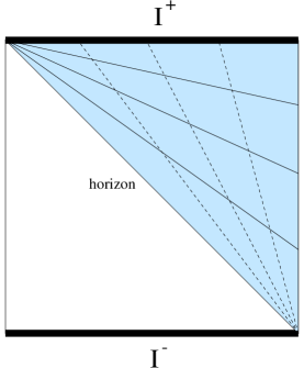
FIG. 1.: Penrose diagram for de Sitter spacetime: Future (Past) Infinity $I^{+}$($I^{-}$) are 3-spheres. The shaded region is that covered by the flat slicing bounded by the horizon of an observer at the origin. Such an observer only sees future infinity $\tilde{I}^{+}$ as an $R^{3}$ ($S^{3}$ minus one point), and only one point at past infinity due to the horizon. The solid lines are surfaces of constant $t$ and the dashed lines are surfaces of constant radius from the origin in the flat slicing.

VII Massless case - flat slicing

The above reasoning does not apply in the $m\rightarrow 0$ limit. As we shall see the asymptotic behaviour in this limit changes. Furthermore the Hadamard function is infinite in the de Sitter vacuum. Despite these problems one can still make sense of this correspondence. A real solution of the equations of motion may be expressed in a complete set of modes

$$\phi(x)=\int\frac{d^{3}k}{(2\pi)^{3}}(a_{k}u_{k}(x)+a^{\dagger}_{k}u^{*}_{k}(x))$$ (45)

with $u_{k}(x)=\frac{H}{\sqrt{2k}}(\eta-\frac{i}{k})e^{-ik\eta+ik.x}$ with $\eta=-e^{-t}$ where $-\infty<\eta<0$. Then one can show that above amplitude is given by

$$(\phi,\phi)=2\int\frac{d^{3}k}{(2\pi)^{3}}|a_{k}|^{2}$$ (46)

Now since the flat slicing modes are well defined in the massless limit then the amplitude is still well defined. The asymptotic behaviour of the modes at future infinity is given by

$$\phi(x,t)=\phi_{-}(x)-\frac{1}{2}e^{-2t}\nabla^{2}\phi_{-}(x)+\phi_{+}(x)e^{-3t}+O(e^{-4t})$$ (47)

It then remains only to relate $a_{k}$ in terms of $\tilde{\phi}_{\pm}(k)$, the Fourier transform of $\phi_{\pm}(x)$. The result is

$$a_{k}=\frac{ik\sqrt{k}}{\sqrt{2}H}\tilde{\phi}_{-}(k)+\frac{3\sqrt{k}}{\sqrt{2}Hk^{2}}\tilde{\phi}_{+}(k)$$ (48)

and so $(\phi,\phi)$ is given by

$$\int d^{3}x\int d^{3}x^{\prime}\phi_{-}(x)D_{+}(x,x^{\prime})\phi_{-}(x^{\prime})+\int d^{3}x\int d^{3}x^{\prime}\phi_{+}(x)D_{-}(x,x^{\prime})\phi_{+}(x^{\prime})$$ (49)

where

$$D_{+}(x,x^{\prime})=\frac{1}{H^{2}}\int\frac{d^{3}k}{(2\pi)^{3}}e^{ik.(x-x^{\prime})}k^{3}=\frac{5!}{2H^{2}\pi^{2}}|x-x^{\prime}|^{-6}$$ (50)

$$D_{-}(x,x^{\prime})=\frac{9}{H^{2}}\int\frac{d^{3}k}{(2\pi)^{3}}e^{ik.(x-x^{\prime})}k^{-3}=c-\frac{9}{H^{2}\pi^{2}}\ln|x-x^{\prime}|$$ (51)

The second correlator $D_{-}(x,x^{\prime})$ exhibits the same infrared divergence as the de Sitter Wightman function, and we have chosen to separate out an infinite constant $c$ to see the physical behaviour. A similar behaviour occurs for a massless field in two dimensions, for instance as occurs in string theory. In that case the divergence comes from the symmetry $X^{\mu}\rightarrow X^{\mu}+a^{\mu}$, i.e. translation invariance on the target space. The result is that $X^{\mu}$ is not a primary operator but its derivatives $\partial X^{\mu}$ are. In the Euclidean formulation where the worldsheet is taken to be an $S^{2}$ the divergence comes entirely from the $L=0$ $S^{2}$ spherical harmonic term and can be projected out, the result is a logarithmic correlation function. In view of these similarities we see that the holographic dual of a massless minimally coupled scalar field in $dS^{d+1}$ contains two conformal fields $O^{+}(x)$ and $O^{-}(x)$, one primary with conformal weight $d$ and correlator $<O^{+}(x)O^{+}(y)>=|x-x^{\prime}|^{-2d}$ and a second non-primary field $O^{-}(x)$, having global symmetry $O^{-}(x)\rightarrow O^{-}(x)+a$ and correlator $<O^{-}(x)O^{-}(y)>=\ln|x-x^{\prime}|$ whose derivatives are primary fields. Alternatively we may in analogy with string theory think in terms of the primary field $\exp[iqO^{+}(x)]$ whose correlator is given by

$$<\exp[iq_{1}O^{-}(x)]\exp[-iq_{2}O^{-}(x)]>=\exp[-\frac{1}{2}q_{1}q_{2}<O^{-}(x)O^{-}(y)>]=|x-x^{\prime}|^{-\frac{1}{2}q_{1}q_{2}}$$ (52)

so that $\exp[iqO^{-}(x)]$ has conformal dimension $q^{2}/4$.

VIII Massless case - closed slicing

In the closed slicing one is free to use either future or past infinity as the boundary. It is unnecessary to use both since the fields at future infinity are completely determined by specifying $\phi^{-}$ and $\phi^{+}$ at past infinity. It is for this reason that only one copy of a CFT is needed. This reflects the fact that the holographic dual of the bulk lives not so much on the boundary but rather on the effective Cauchy surface. We shall define the holographic dual at future infinity for ease of comparison with the flat slicing case. In order to give a finite amplitude we choose a $\phi(x)$ such that

$$\int\frac{\partial\phi(x)}{\partial\tau}d\Omega_{S^{3}}=0$$ (53)

It is significant that the $L=0$ mode has not been included. This allows us to work with manifestly finite expressions. The asymptotic behaviour at future infinity is

$$\phi(x,\tau)=\phi_{-}(x)-2e^{-2\tau}\nabla^{2}\phi_{-}(x)+\phi_{+}(x)e^{-3\tau}+O(e^{-4\tau})$$ (54)

Ignoring the contributions form the $L=0$ modes the asymptotic form of the Hadamard function is

$$G^{h}(x,\tau;x^{\prime},\tau^{\prime})=\frac{H^{2}}{4\pi^{2}}(-\ln\sigma+(1-\frac{2}{\sigma})(e^{-2\tau}+e^{-2\tau^{\prime}})-4(\frac{1}{\sigma^{2}}+\frac{1}{\sigma})e^{-2(\tau+\tau^{\prime})}+\frac{128}{3\sigma^{3}}e^{-3(\tau+\tau^{\prime})})$$ (55)

to order $O(e^{-4\tau},e^{-4\tau^{\prime}})$. Then

$$(\phi,\phi)=c_{+}\int d\Omega_{S^{3}}\int d\Omega^{\prime}_{S^{3}}\phi_{-}(x)\frac{1}{\sigma^{3}}\phi_{-}(x^{\prime})+c_{-}\int d\Omega_{S^{3}}\int d\Omega^{\prime}_{S^{3}}\phi_{+}(x)\ln\sigma\phi_{+}(x^{\prime})$$ (56)

where $c_{\pm}$ are constants. Note that the infinite constant that occurred in the flat slicing correlator has been automatically projected out by imposing the condition (e.q. 16). As expected this is simply the flat slicing result conformally transformed to the 3-sphere.

IX Conclusion

In this paper we have shown how to consistently quantize the massless minimally coupled scalar field on de Sitter spacetime for the de Sitter invariant vacuum. We have shown that this is equivalent to the Euclidean vacuum as for the massive case. This treatment shows the different but nevertheless equivalent ways global symmetries are treated in Lorentzian and Euclidean formulations of field theory. We have shown that as for the massive case the massless minimally coupled scalar field also has a CFT interpretation as a conformal field with weight $d$ and a second field with a logarithmic correlator. The second field exhibits the same global symmetry and infrared divergence as the massless field in de Sitter and we argue that this apparent problem should have the same resolution, namely that one should think in terms of physical correlators for which the infrared divergence is removed. It is well known that the graviton in de Sitter spacetime considered in physical gauge in the flat slicing behaves like a massless minimally coupled scalar field [16] and so we anticipate that a similar approach will be needed in this case.

Acknowledgements: We thank C. Galfard and T. Wiseman for useful discussions. AJT acknowledges the support of an EPSRC studentship. The work of NT is supported by PPARC (UK).

X Appendix

De Sitter spacetime can be defined as the hyperboloid $x\cdot x=H^{-2}$ embedded in a 5 dimensional flat manifold with signature $(-++++)$, where ‘$\cdot$’ denotes the $SO(1,4)$ invariant inner product. The constant ‘$H$’ is the Hubble constant viewed from the flat slicing. The curvature is given by $R=12H^{2}$. The distance between two points in the embedding space $(x-y)\cdot(x-y)$ provides a de Sitter invariant metric. It is usual to define the quadratic form $z(x,y)$ through $\frac{H^{2}}{2}(x-y)^{2}=(1-z(x,y))$, so that $z(x,y)=H^{2}x\cdot y$. If $z>1$ ($<1$) the points are timelike (spacelike) separated.

The closed co-ordinate system is obtained through the embedding procedure by the identification $(x^{0},x^{i})=(H^{-1}\sinh\tau,H^{-1}n^{i}\cosh\tau)$ where $n^{i}n_{i}=1$ defines an $S^{3}$. Explicitly $n^{i}=(\sin\chi\sin\theta\cos\phi,\sin\chi\sin\theta\sin\phi,\sin\chi\cos\theta,\cos\chi)$. The de Sitter invariant measure, or volume element, in this co-ordinate system is given by

$$dV=\sqrt{-g}d^{4}x=H^{-4}(\cosh\tau)^{3}d\tau d\Omega_{S^{3}}$$ (57)

where $d\Omega_{S^{3}}=\sin^{2}\chi\sin\theta d\chi d\theta d\phi$ is the volume element on $S^{3}$. The invariant distance between two points on $S^{3}$, used in the text, is defined by $\sigma(x,x^{\prime})=\frac{1}{2}|n^{i}-{n^{i}}^{\prime}|^{2}=1-n^{i}n_{i}^{\prime}$.

The Klein-Gordon inner product is given by

$$\langle\phi,\psi\rangle=\frac{i}{H^{2}}\int_{\Sigma}(\cosh\tau)^{3}(\phi^{*}\partial_{\tau}\psi-\psi^{*}\partial_{\tau}\phi)d\Omega_{S^{3}}$$ (58)

In the scalar representation of $SO(1,4)$, the generators are

$$M_{AB}=i[x_{A}\frac{\partial}{\partial x^{B}}-x_{B}\frac{\partial}{\partial x^{A}}].$$ (59)

In addition to the $SO(4)$ generators $M_{ij}$ associated with the isometry group of the $S^{3}$, one has the non-compact generators

$$M_{0i}=-in_{i}\frac{\partial}{\partial\tau}-i\tanh\tau[\frac{\partial}{\partial n^{i}}-n^{i}n^{j}\frac{\partial}{\partial n^{j}}],$$ (60)

and so

$$\hat{Z}=i\frac{x^{i}}{\sqrt{x^{i}x_{i}}}M_{0i}=in^{i}M_{0i}=\frac{\partial}{\partial\tau}.$$ (61)

The analytic continuation from de Sitter spacetime to $S^{4}$ is achieved by continuing $\tau\rightarrow-iX$ on the matching surface $\tau=X=0$. This yields the Euclidean metric

$$ds^{2}=H^{-2}(dX^{2}+\cos^{2}X(d\chi^{2}+\sin^{2}\chi(d\theta^{2}+\sin^{2}\theta d\phi^{2})))$$ (62)

with $-\pi/2<X<\pi/2$. Distances on the $S^{4}$ are defined via $Z(x,y)=H^{2}x\cdot y$, just as in the de Sitter case but now using the $O(5)$ invariant metric on the flat embedding space.

REFERENCES

- [1] Allen and Folacci, Phys. Rev. D 35, 3771-3778 (1987); Allen, Phys. Rev. D 32, 3136-3149 (1985).
- [2] E. Witten, hep-th/0106109.
- [3] A. Strominger, J. High Energy Phys. 0110, 034 (2001).
- [4] C.M. Hull, J. High Energy Phys. 9807, 021 (1998).
- [5] P.O. Mazur, E. Mottola, Phys. Rev. D 64, 104022 (2001); D. Klemm, Nucl. Phys. B625, 295-311 (2002); S. Nojiri, S.D. Odintsov, Phys. Lett. B519, 145-148 (2001); T. Shiromizu, D. Ida,T. Torii, J. High Energy Phys. 0110, 010 (2001).
- [6] J. Maldacena, C. Nunez, Int. J. Mod. Phys. A16, 822-855 (2001).
- [7] T. Banks, Int. J. Mod. Phys. A16, 910-921 (2001).
- [8] Kirsten and Garriga, Phys. Rev. D 48, 567-577 (1993).
- [9] J.P. Gazeau, J. Renaud, M.V. Takook, Class.Quant.Grav. 17, 1415-1434 (2000).
- [10] J. Bros, H. Epstein, U. Moschella, Phys. Rev. D 65, 084012 (2002).
- [11] J.B. Hartle, S.W.Hawking Phys. Rev. D 28, 2960-2975 (1983).
- [12] N.D. Birrell and P.C.W. Davies, Quantum fields in curved space, (Cambridge University Press, Cambridge, England, 1984).
- [13] Robert M. Wald, Quantum Field Theory in Curved Spacetime and Black Hole Thermodynamics (University of Chicago Press, Chicago, 1994).
- [14] N. Vilenkin, Special functions and theory of group representations (American Mathematical Society, 1983).
- [15] J. Maldacena, Int. J. Theor. Phys. 38, 1113-1133 (1999).
- [16] N.C. Tsamis, R.P. Woodard, Class.Quant.Grav. 11, 2969-2990 (1994).
- [17] C.M. Hull, J. High Energy Phys. 0111, 012 (2001); C.M. Hull, J. High Energy Phys. 0111, 061 (2001); G.W. Gibbons, C.M. Hull, hep-th/0111072; P. Fre, M. Trigiante, A. Van Proeyen, hep-th/0205119; R. Kallosh, hep-th/0205315; A. Maloney, E. Silverstein, A. Strominger, hep-th/0205316.
- [18] D. Klemm, L. Vanzo, J. High Energy Phys. 0204, 030 (2002); E. Halyo, hep-th/0203235; A.J.M. Medved, hep-th/0203191; F. Larsen, J.P. van der Schaar, R.G. Leigh, J. High Energy Phys. 0204, 047 (2002); A.J.M. Medved, Class.Quant.Grav. 19, 2883-2896 (2002); M. Spradlin, A. Volovich, Phys. Rev. D 65, 104037 (2002); R. Bousso, A. Maloney, A. Strominger, Phys. Rev. D 65, 104039 (2002); V. Balasubramanian, J. de Boer, D. Minic, Phys. Rev. D 65, 123508 (2002); A. Strominger, J. High Energy Phys. 0111, 049 (2001); M. Spradlin, A. Strominger, A. Volovich, hep-th/0110007.