Lab/UFR-HEP/0109
NC Branes and Hierarchies
in Quantum Hall Fluids

Abstract

We develop the non commutative Chern-Simons gauge model analysis modeling the description of the hierarchical states of fractional quantum Hall fluids. For a generic level $n$ of the hierarchy, we show that the order parameter matrix $K_{ab}$ is given by $\theta^{-2}Tr(\tau_{a}\tau_{b})$, where $\{\tau_{a},1\leq a\leq n\}$ define a specific set of $n\times n$ matrices depending on the parameter $\theta$ and the levels $l_{a}$ of the CS effective field theory. Our analysis predicts the existence of a third order tensor of order parameters $C_{abc}$ induced by the external magnetic field. It is shown that the $C_{abc}$’s are not new order parameters and are given by $\theta d_{abc}$, where $d_{abc}$ are numbers depending on the $l_{a}$’s. We also give the generalized quantum Hall soliton extending that obtained in the case of the Laughlin state.

Key Words: Branes physics, NC Chern-Simons gauge theory, Fractional Quantum Hall fluids, Hierarchical states and Matrix model.

1 Introduction

Recently it has been proposed that non-commutative (NC) Chern-Simons gauge theory on the $(2+1)$ space may provide a description of the Laughlin state of Fractional Quantum Hall (FQH) fluids [1-6]. In this context, it has been shown that the non commutativity parameter $\theta$ of the Moyal plane is related to the filling fraction $\nu_{L}$ of the Laughlin state and so to the Chern-Simon effective field coupling $\lambda_{CS}$ as $\theta B\nu_{L}=\nu_{L}\lambda_{CS}=1$; with $B$ the external magnetic field and the subscript L stands for Laughlin. In [7], see also [8-11], it has been also conjectured that a specific assembly of a system of $D0$, $D2$ and $D6$ branes and $F1$ strings, stretching between $D2$ and $D6$, has a low energy dynamics similar to the fundamental state of FQH systems. There, the boundary states of the F strings ending on the NC D2 brane are interpreted as the FQH particles. In an external strong magnetic field $B$, represented by a large number of D0 branes dissolved in D2, the dynamics of these particles is modeled by a non commutative Chern-Simons (NCCS) $U(1)$ gauge field theory.

In this paper we use these results to develop the NC Chern-Simon theory modeling the description of the hierarchical states of FQH systems. The point is that FQH systems with general expressions of the filling fraction $\nu$ are not all of them of Laughlin type [12]; i.e with filling fraction $\nu_{L}=\frac{1}{m}$, $m$ odd integer. Typical examples are given by states with $\nu(l_{1},l_{2})=\frac{l_{2}}{l_{1}l_{2}-1}$ where $l_{1}$ and $l_{2}$ are respectively odd and even integers. These kind of states are approached using hierarchical construction ideas [13-25]. In the hydrodynamical approach of FQH fluids, the $\frac{l_{2}}{l_{1}l_{2}-1}$ state can be viewed as consisting of two components of incompressible fluids; one describing $\nu_{L,1}=\frac{1}{l_{1}}$ FQH state while the other describes the condensation of quasiparticles on the top of the $\nu_{L,1}=\frac{1}{l_{1}}$. Put differently, the $\frac{l_{2}}{l_{1}l_{2}-1}$ state can be imagined as a composed system of a Laughlin state of filling fraction $\nu_{L,2}=\frac{1}{l_{1}(l_{2}l_{1}-1)}$ built on an other one with $\nu_{L,1}=\frac{1}{l_{1}}$ and satisfying the identity $\nu(l_{1},l_{2})=\nu_{L,1}+\nu_{L,2}$. As such the total number of particles can, roughly speaking, be thought of as given by the sum $N_{1}+N_{2}$, where $N_{1}$ is associated with the state of filling fraction $\nu_{L,1}$ and $N_{2}$ with the state $\nu_{L,2}$; see ${\it figures}$ 3 and 4 of section 4. These features apply as well for higher orders of the hierarchy with $\nu=\nu(l_{1},l_{2},...,l_{n})$. Current examples correspond to $\nu(3,2)=\frac{2}{5}=\frac{1}{3}+\frac{1}{15}$ and $\nu(3,2,2)=\frac{3}{7}=\frac{1}{3}+\frac{1}{15}+\frac{1}{35}$.

In the field theory approach, the hierarchical states we refer to here above are described by a $(2+1)$ dimensional system of coupled CS gauge fields whose action reads for generic levels $n$ as, [26,27,28]

$$S=\frac{1}{4\pi}\int d^{3}y\ K_{ab}\partial_{\mu}A_{\nu}^{a}A_{\rho}^{b}\epsilon^{\mu\nu\rho}+J_{a}^{\mu}A^{a}_{\mu}.$$ (1)

In this eq $K_{ab}$ is a $n\times n$ matrix with specific integer entries defining the order parameters characterizing the fluid and carrying the interactions between the CS gauge fields. $J_{a}^{\mu}$’s are external charge density currents linked for $n=1$ with the D6 branes charge of the quantum Hall soliton [7,8]. Note that for this case, the above gauge model reduces to the usual CS effective field theory of the Laughlin state with filling fraction $\nu_{L}=K_{11}^{-1}={1\over m}$. For $n=2$, however, one deals with a FQH system with filling fraction $\nu(l_{1},l_{2})=\frac{l_{2}}{l_{1}l_{2}-1}$ and so with hierarchical states of level two. In the Haldane model where $\nu(l_{1},l_{2})$ may be decomposed as the sum over $\nu_{L,1}$ and $\nu_{L,2}$, the $K_{ab}$ matrix reads then as:

$$K_{ab}=\left(\matrix{(2P_{1}+1)&-1\cr-1&2P_{2}\cr}\right)$$ (2)

where we have set $l_{1}=2P_{1}+1$ and $l_{2}=2P_{2}$. Notice that because of the property $K_{12}\neq 0$; there exists a non trivial coupling between the two $A^{1}_{\mu}$ and $A^{2}_{\mu}$ CS gauge fields. This feature will play a crucial role in our present study especially when we build the NCCS theory describing hierarchies by generalizing Susskind method .

Throughout this study we will discuss in details the above mentioned level two Haldane states by developing an adequate generalization of the Susskind construction performed for the Laughlin model. We will also study the case of generic levels of Haldane other hierarchies. Moreover we build the generalization of the quantum Hall soliton and give an interpretation of FQH hierarchies in terms of $Dp$ branes of uncompactified type IIA string theory.

The presentation of this paper is as follows. In section 2 we develop the matrix model used to describe level two hierarchical states of FQH liquids with a finite number $N$ of particles. In section 3, we study the NCCS gauge model for the case of Haldane states at level two and consider the infinite limit of $N$ where one dimensional matrix fields are mapped to (2+1)dimensional fields. In this limit the $U(N)$ symmetry is replaced by $SDiff(R^{2})$, the group of area preserving diffeomorphisms of the $R^{2}$ plane while the matrix commutator becomes a Poisson bracket. In section 4 we build the generalized quantum Hall soliton describing hierarchical states while in section 5 we give results concerning generic values of the level $n$ of the hierarchy. Section 6 is deserved for conclusion.

2 Hierarchy and Matrix Model for FQH states

In this section we will construct a non-commutative gauge model for the description of hierarchical states of FQH liquids. This model is based on an extension of the Susskind analysis made for the case of the Laughlin state. We first consider the case of a finite number $N$ of electrons; then we aboard the interesting limit when $N$ goes to infinity. The determination of the standard CS effective field theory as the leading term in the NC parameter $\theta$ will be worked out explicitly.

To establish the matrix model for the description of FQH hierarchies, we will adopt the following strategy: First we consider a toy model, a matter of introducing some general tools useful for the next steps. Second we develop our matrix model for the description of hierarchical states of level two for a system of $N_{1}+N_{2}=2N$ electrons and finally consider the limit $N$ goes to infinity.

2.1 General

To begin consider an electric charged particle, say an electron, moving in the real plane in presence of an external constant magnetic field $B$. Classically this particle is parametrized by its position $x^{i}(t);\ i=1,2$ and velocity $v^{i}=\partial_{t}{x^{i}}$. For a $B$ field strong enough, the dynamics of the particle is mainly governed by the coupling

$$S[x]=\frac{eB}{2}\int dt{\varepsilon_{ij}v^{i}x^{j}},$$ (3)

which induces at the quantum level a non commutativity structure on the real plane; i.e $[x^{i},x^{j}]\propto\epsilon^{ij}/B$. In the case of $N$ classical particles, without mutual interactions, parameterized by the coordinates $x^{i}_{a}(t)$ and velocities $v^{i}_{a}$, the dynamics is dominated by the $B-x(t)$ couplings extending eq(3) as $eB\ \varepsilon_{ij}\ \Sigma_{a=1}^{N}v^{i}_{a}x^{j}_{a}$ and describing a typical strongly correlated system of electrons showing a quantum Hall effect of filling fraction $\nu=\frac{N_{e}}{N_{\phi}}$; where $N_{\phi}=\int_{S^{2}}B$ and $N_{e}=N$ are respectively the quantum flux and electrons numbers. Quantum mechanically, there are different field theoretical methods to approach the quantum states of this system [20], either by using techniques of non relativistic quantum mechanics [12], methods of conformal field theory especially for the study of the edge excitations[14,15] or again by using the CS effective field model [16] describing the limit $N\rightarrow\infty$ of electrons. In this case, the CS theory on the $(2+1)$ dimensional space modeling the FQH Laughlin state of filling fraction $\nu$ is given by the following action:

$$S[A]=\frac{1}{4\pi\nu}\int d^{3}y\epsilon^{\mu\nu\rho}\partial_{\mu}A_{\nu}A_{\rho}+\int d^{3}yJ^{\mu}A_{\mu},$$ (4)

The link between this field action and FQH fluids dynamics has been studied in details and most of the results in this direction has been established several years ago [5-18]. However an interesting observation has been made recently by Susskind [1] and further considered in [2-6] and [8-11]. The novelties brought by the study made in [1] is that: (1) Because of the $B$-field, level $n$ NC Chern-Simons $U(1)$ gauge theory may provide a description of the Laughlin theory at filling fraction $\nu_{L}=\frac{1}{m}$. In this vision, Eq(4) appears then just as the leading term of a more general theory which reads in general as:

$$S[A]=\frac{1}{4\pi\nu}\int d^{3}y\epsilon^{\mu\nu\rho}[\partial_{\mu}A_{\nu}\ast A_{\rho}+\frac{2i}{3}A_{\mu}\ast A_{\nu}\ast A_{\rho}]+\int d^{3}yJ^{\mu}A_{\mu},$$ (5)

where $\ast$ stands for the usual star operation of non commutative field theory [29]. (2) The above NCCS $U(1)$ action is in fact the $N\rightarrow\infty$ of the following matrix model action:

$$S=\frac{eB}{2}\int dt(\epsilon_{ij}\sum_{\alpha=1}^{N}[(\dot{X}^{i}+i[A_{0},X^{i}])X^{j}+\theta\epsilon^{ij}A_{0}]_{\alpha,\alpha}),$$ (6)

by substituting the $X^{i}_{\alpha\beta}$’s as:

$$X^{i}_{\alpha\beta} = y^{i}\delta_{\alpha\beta}+\theta\varepsilon^{ij}(A_{j})_{\alpha\beta},$$ (7)

$$[y^{i},y^{j}] = i\theta\varepsilon^{ij}.$$ (8)

At this stage let us give some remarks, they concern some remarkable properties of the above analysis that we will not have the occasion to address in the present paper: (a) The finite matrix model (6), which has been conjectured in [17] to describe fractional quantum Hall droplets, was shown to be equivalent to the Calogero integrable model [30] providing then another link between Calogero and Hall systems. (b) The mapping (7), which is interpreted as describing fluctuations carried by $A_{j}$ around the classical solution $X^{i}=y^{i}I$, is a kind of background field splitting. It is formally similar to the gauge splitting one uses in the derivation of matrix model from the ten dimensional Super Yang-Mills theory [31] by using dimensional reduction from $(1+9)$ down to $(1+0)$. Note that in the ideal case where $N=1$, eq(6) reduces to eq(3) with the constraint eq(8); this ideal situation will be shown later on to be just the leading term of a hierarchical series; see eq (9) and eq(45).

The analysis we gave here above concerns the Laughlin state; the fundamental state of FQH systems. In what follows we want to generalize it to include hierarchical states. We will start by considering quantum states of level two and too particularly those having a filling fraction $\nu_{H}(l_{1},l_{2})=\frac{l_{2}}{l_{1}l_{2}-1}$. Later we turn to the general case.

2.2 1D NC $U(2)$ gauge model

In the purpose of studying FQH states with $\nu_{H}(l_{1},l_{2})$, let us first consider a toy model where the $X^{i}(t)=(X^{1},X^{2})$ are two one dimensional 2$\times$2 hermitian matrix fields whose dynamics, in the strong B regime, is described by the following action:

$$S=\frac{eB}{2}\int dt\ \epsilon_{ij}\ Tr_{u(2)}\ [(\dot{X}^{i}+i[A_{0},X^{i}])X^{j}+\theta\epsilon^{ij}A_{0}]$$ (9)

In this eq $A_{0}=A_{0}(t)$ is a one dimensional (1D) gauge field valued in the $U(2)$ algebra; naively it may be thought of as the time component of the $U(1)$ CS gauge field to be considered later on. To fix the idea, the above action may be viewed as associated with the leading term of a general formula; see eq(20).

Since $U(2)=U(1)\times SU(2)$, only the $U(1)$ gauge factor of the gauge field will contribute in the second term of the action(9). This action depends linearly on $A_{0}$ and so it is just a Lagrange field carrying a field constraint which can be determined by calculating its equation of motion. In doing so, we get the following action of the $X^{i}(t)$’s fields

$$S=\frac{eB}{2}\int dt\epsilon_{ij}Tr_{u(2)}(\dot{X}^{i}X^{j}),$$ (10)

together with the $2\times 2$ matrix constraint equation,

$$[X^{i},X^{j}]=i\theta\epsilon^{ij}I_{2}.$$ (11)

Expanding the $X^{i}(t)$ field matrix as follows:

$$X^{i}=X^{i}_{0}I_{2}+Z^{i}_{a}\sigma^{a},$$ (12)

where $I_{2}$ stands for the $2\times 2$ identity matrix and $\sigma^{a}=(\sigma^{x},\sigma^{y},\sigma^{z})$ are the usual Pauli matrices. Splitting the $X^{i}_{0}(t)$ field component, associated with the $U(1)$ factor of $U(2)$, as a sum of constant $y^{i}$ and a term dependent on time as:

$$X^{i}_{0}(t)=(y^{i}+Z^{i}_{0}(t))I_{2},$$ (13)

then putting $X^{i}=y^{i}I_{2}+Z^{i}$ back into eq(11), we get the following algebra,

$$\matrix{[y^{i},y^{j}]=i\theta\epsilon^{ij}&&(1)\cr[y^{i},Z^{j}]=0&&(2)\cr[Z^{i},Z^{j}]=0&&(3)\cr}$$ (14)

Eqs (14.2-3) may be further decomposed using the properties of the Pauli matrices, in particular the Clifford and the su(2) algebraic relations. We find,

$$[y_{i},Z_{a}(t)] = 0\ \ ,\ \ a=0,1,2,3.$$ (15)

$$\sum_{a=0}^{3}[Z_{a}^{i},Z_{a}^{j}]I_{2}+i\sum_{a,b,c=1}^{3}\varepsilon^{abc}Z^{i}_{a}Z^{j}_{b}\sigma^{c} = 0.$$ (16)

A natural solution of these eqs is obtained by taking $Z_{a}(t)=0,\ a=0,1,2,4$, so that eq(14-1) describes just the classical solution. Therefore the $Z_{a}^{i}(t)$ fields appearing in eqs(12-13) are interpreted as describing fluctuations around the classical configuration $X^{i}=y^{i}I_{2}$. To get the action describing the $Z_{a}^{i}(t)$ fluctuations, we substitute the $X^{i}(t)$’s by the splitting (12) and use eq(14-1), we get

$$S=\frac{eB}{2}\int dt\epsilon_{ij}Tr_{U(2)}[(\dot{Z}^{i}+i[A_{0},Z^{i}])Z^{j}.$$ (17)

This action is invariant under $U(2)$ automorphisms of the matrix fields, namely

$$Z^{i\prime}=U^{+}Z^{i}U$$

$$A_{0}^{\prime}=U^{+}A_{0}^{i}U-iU^{+}{\partial\over\partial t}U.$$ (18)

Eq(17) may be generalized by including fermions that we have ignored here above as they are not needed in the present study; it may also be extended by using, instead of $2\times 2$ matrices, higher dimensional matrix fields. We will consider this situation in section 5 when we consider FQH states with filling fraction $\nu_{H}(l_{1},l_{2},...,l_{n})$. One of the extensions we are interested in here, which will be used to describe FQH states at level two of hierarchy (SL2 for short), is based on taking hermitian field matrix valued in the $u(2)\oplus u(N)$.

3 NC Gauge Model for Haldane States

To start consider the system of $N_{1}+N_{2}$ electrons on the real plane parameterized by the coordinates $y^{i}=(y^{1},y^{2})$. $N_{1}$ should be thought as the number of electrons associated with the underlying Laughlin state of filling fraction $\nu_{L,1}=\frac{1}{l_{1}}$. $N_{2}$ is a priori the number of particles we get after condensation of quasiparticles [5,21]; it can be thought of as associated with the filling fraction $\nu_{L,2}=\nu_{H}(l_{1},l_{2})-\nu_{L,1}=\frac{1}{l_{1}(l_{1}l_{2}-1)}$. For reasons of simplicity of the formulation of our effective model, we will suppose that $N_{1}=N_{2}=N$ and consider the case of configurations with a finite number $2N$ of electrons whose coordinates are represented by $2N\times 2N$ dimensional hermitian matrices $X^{i}(t)$. These are one dimensional fields valued in the adjoint representation of $U(2)\oplus U(N)\subset U(2N)$. Put differently, the $X^{i}$ fields have an expansion generalizing eq(12) in the sense that each component $Z_{a}$ is itself a $N\times N$ hermitian matrix valued adjoint of the group $U(N)$:

$$Z^{i}_{a}=\sum_{B}T_{B}Z_{a}^{i,B}(t),$$ (19)

where the $T_{B}$’s are the $U(N)$ generators. The new matrix model describing the dynamics of SL2, in presence of a strong B field, has an action formally similar to eq (6), except now that the $X^{i}(t)$ and $A_{0}(t)$ fields are in $Adj_{U(2)\oplus U(N)}$ and the trace is taken over the states of the $u(2)\oplus u(N)$ algebra. Thus we have,

$$S=\frac{1}{g^{2}_{2}}\int dt\epsilon_{ij}Tr_{(u(2)\oplus u(N))}[(\dot{X}+i[A_{0},X^{i}])X^{j}+\theta\epsilon^{ij}A_{0}(1+J_{0})],$$ (20)

where $J_{0}$ is the current density of a given external source and where $g_{2}$ is a coupling constant to be determined later on; it carries informations on the SL2 filling fraction $\nu$ and the non commutativity parameter $\theta$. The action (20) is symmetric under the following change extending eq(18)

$${X}^{i\prime}={\it W}^{+}{X}^{i}{\it W}$$

$$A_{0}^{\prime}={\it W}^{+}A_{0}{\it W}-i{\it W}^{+}{\partial\over\partial t}{\it W},$$ (21)

where${\it W}=U\otimes V$, is a unitary transformation of the $U(2)\otimes U(N)$ gauge group. Setting $U=exp{(i\sum_{a=1}^{3}\lambda_{a}\sigma^{a})}$ and $V=exp(i{\sum_{B=1}^{n^{2}}\Lambda_{B}T^{B})}$, the infinitesimal form of the transformations eq(21) reads for the case of $U(N)$ gauge symmetry for instance as:

$$\delta X^{i} = -i[y^{i},\Lambda]-i[A,X^{i}]$$

$$\delta A_{0} = {\partial\over\partial t}\Lambda+i[\Lambda,A_{0}]$$ (22)

Before going ahead note that due to eq(14.1), $[y^{i},\Lambda]$ behaves as a derivation since,

$$[y^{i},\Lambda]=i\theta\epsilon^{ij}\partial_{j}\Lambda.$$ (23)

In the limit $N$ goes to infinity the one dimensional $2N\times 2N$ fields $X^{i}(t)$ and $A_{0}(t)$ become infinite matrices; they may be represented by (2+1) dimensional field $X^{i}(t,y^{1},y^{2})$ and $A_{0}(t,y^{1},y^{2})$ and so is the $Z^{i}$ fluctuations around the classical solution; all of them are valued in the $U(2)$ algebra. For later use let us expand this field in terms of the $U(2)$ generators as,

$$Z^{i}(y)=Z^{i}_{0}(y)I_{2}+\sum_{a=1}^{3}Z^{i}_{a}(y)\sigma^{a}.$$ (24)

Moreover when $N\longrightarrow\infty$ the $U(2)\otimes U(N)$ symmetry is also mapped to $U(2)\times SDiff(R^{2})$; $SDiff(R^{2})$ being the area preserving diffeomorphism group of $R^{2}$ plane. So the $Z^{i}(t,y^{1},y^{2})$ fluctuations around the classical solution $y^{i}I$ should be proportional to the space components $A_{j}(y)$ of the $U(1)$ Chern-Simons gauge field as

$$Z^{i}(y)\propto\epsilon^{ij}A_{j}(y).$$ (25)

Since the $Z^{i}(y)$ fluctuations scale as [Z]=[X]=[y]=L while the gauge field $A_{j}$ scales as $L^{-1}$, the factor of proportionality should scale like [X]/[A]=$L^{2}$ as $\theta$ does. Here below we study these fluctuations and derive the extension of eq(7) for the case of SL2.

3.1 Generalized Susskind map

In the decomposition (24) involving the dimensionless Pauli matrices, the scaling behaviour of $X$ is completely carried by the $Z_{a}^{i}$ component fields. To convert this expansion in term of the $A^{i}$ gauge fields scaling as $(length)^{-1}$, it is convenient to introduce a new vector basis $\{\tau^{1},\tau^{2},\tau^{3}\,\tau^{4}\}$ of $U(2)$ related to the standard Pauli matrices basis $\{\sigma^{x},\sigma^{y},\sigma^{z},\sigma^{4}\equiv I_{2}\}$ as:

$$\tau^{a}=\sum_{b=1}^{4}\ \Gamma^{a}_{b}\ \sigma^{b}\qquad;\qquad a,b=1,2,3,4.$$ (26)

where the entries of the invertible $4\times 4$ matrix $\Gamma$ scale as $(length)^{2}$. This change of basis turns out to be very useful when studying the order parameters of FQH fluids; see eqs (32) and (34). To fix the ideas, let us give hereafter the following special choice for $\tau_{1}$ and $\tau_{2}$ in terms of $\sigma^{a}$’s,

$$\tau_{1} = [\ \alpha_{0}I+\alpha_{1}\sigma^{x}+\alpha_{2}\sigma^{y}\ ],$$

$$\tau_{2} = [\ -\alpha_{1}\sigma^{x}-\alpha_{2}\sigma^{y}+\alpha_{3}\sigma^{z}\ ],$$ (27)

where we have set $\alpha_{1}=\Gamma^{1}_{1}=-\Gamma^{2}_{1},\ \alpha_{2}=\Gamma^{1}_{2}=-\Gamma^{2}_{2},\ \alpha_{3}=\Gamma^{2}_{3}$ and $\alpha_{0}=\Gamma^{4}_{4}$. Similar formulas may be worked out for $\tau_{3}$ and $\tau_{4}$, but we don’t need them for the present study. We will show later that the $\alpha_{a}$ parameters in the above eqs are related to the $l_{1}$ and $l_{2}$ order parameters of the SL2 configurations and to the non commutativity parameter $\theta$ of the plane. Using this $\tau$ vector basis, we can expand the gauge fields as

$$A_{i}(y)=\tau_{1}A^{1}_{i}(y)+\tau_{2}A^{2}_{i}(y)+\tau_{3}A^{3}_{i}(y)+\tau_{4}A^{4}_{i}(y),$$ (28)

which upon substituting eq(26), we get the right relation between the $Z$ and $A$ fluctuations.

To get the infinitesimal gauge transformations(22), we have to make use of the correspondence rules mapping infinite matrices algebra to the space of functions on the plane. Among them we set:

(i) In the infinite limit, $N\times N$ matrix commutators $[F(t),G(t)]_{\alpha\beta}$ are replaced by the Poisson bracket $\{F(y),G(y)\}=\varepsilon^{kl}\partial_{k}F\partial_{l}G$. In other words,

$$\lim_{N\rightarrow\infty}{i}[F(t),G(t)]\rightarrow\theta\ \varepsilon^{kl}\ \ \frac{\partial F(t,y)}{\partial{y}^{k}}\ \frac{\partial G(t,y)}{\partial{y}^{l}}.$$

So that the infinitesimal gauge transformation reads as,

$$\delta A_{\mu}=\partial_{\mu}\Lambda+\theta\{\Lambda,A_{\mu}\}+0(2).$$ (29)

(ii) the trace $Tr_{U(2)\otimes U(N)}$ operation over the $U(2)\otimes U(N)$ adjoint representation states is mapped for $N\rightarrow\infty$, to $\int d^{2}yTr_{U(2)}$; $lim_{N\rightarrow\infty}Tr_{U(N)}$ should be thought of as $\int d^{2}y$. Therefore we have, after setting $t=y^{0}$ and associating the Dirac delta function $\delta^{2}(y)$ to the $N\times N$ identity matrix $I_{N}$, the following correspondence:

$$\lim_{N\rightarrow\infty}\ \frac{1}{N}\int dt\ Tr_{U(2)\otimes U(N)}[...](t)\ \rightarrow\ \int d^{3}y\ Tr_{U(2)}[...](y).$$

Starting from eq(20) and taking $N\rightarrow\infty$, the one dimensional infinite matrix $X(t)$ is mapped to the $(1+2)$ function $X(t,y)=y+A(t,y)$, where $A(t,y)$ is a gauge field valued in the $U(2)$ algebra. Putting back the above expression into eq(20) and following the same analysis made in [1], we get after replacing $Tr_{U(N)}\rightarrow\int d^{2}y$, the following NC Chern-Simon gauge theory with a non abelian $U(2)$ gauge group.

$$S=\frac{1}{4\pi g^{2}_{2}}\int d^{3}y\ \ \epsilon^{\mu\nu\rho}\ Tr_{U(2)}[\partial_{\mu}A_{\nu}A_{\rho}-\frac{1}{3}A_{\mu}\{A_{\nu},A_{\rho}\}]+{\cal O}(2)$$ (30)

Like in the Susskind analysis, the ${\cal O}(2)$ terms carry higher corrections in the NC parameter which can be obtained by expanding the star product in eq(5). Here we will ignore this detail and so forget about it. The above action is quite similar to eq(1) that we are looking for. A careful inspection shows that eq(30) is not convenient to describe states of level two of the hierarchy as it contains a non abelian gauge symmetry which is not allowed for the study of FQH hierarchies. In other words the expansion(28) and so eq(30) contain too much degrees of freedom, too much more than those appearing in eq (1). They should be then reduced down to two gauge fields only.

Comments

At first sight, the problem of keeping two gauge fields $B$ and $B^{{}^{\prime}}$ amongst the four $U(2)$ gauge ones;

$${\bf B}=BY+B^{+}\sigma^{-}+B^{-}\sigma^{+}+B^{{}^{\prime}}\sigma^{3},$$

$Y$ is the generator of the $U(1)$ factor of $U(2)$, is not a major task in gauge theory with matter. Massless and neutral gauge fields are obtained by breaking $U(2)$ gauge group down to its Cartan subgroup $U(1)^{2}$. The two other gauge fields; that is the $B^{\pm}$ fields associated with the $U(2)$ step generators $\sigma^{\pm}$, acquire masses which by an appropriate choice of the Higgs vacuum moduli may be supposed to be heavy enough and then integrated out by eliminating $B^{\pm}$ through their equations of motion; that is: $B^{+}=B^{+}(B,B^{{}^{\prime}},B^{-};\partial B,\partial B^{{}^{\prime}},\partial B^{-})$ and $B^{-}=B^{-}(B,B^{{}^{\prime}},B^{+};\partial B,\partial B^{{}^{\prime}},\partial B^{+})$. As a result one gets an effective field theory depending only on the $B$ and $B^{{}^{\prime}}$ massless fields. Interactions between $B$ and $B^{{}^{\prime}}$, which are generally absent in $U(1)\times U(1)$ theories, might come here from the substitution of $B^{+}=B^{+}(B,B^{{}^{\prime}},B^{-};\partial B,\partial B^{{}^{\prime}},\partial B^{-})$ and $B^{-}=B^{-}(B,B^{{}^{\prime}},B^{+};\partial B,\partial B^{{}^{\prime}},\partial B^{+})$; but this issue still needs a deeper study. In the brane language, this consists to have a large splitting of the two D2 branes and so too completely separate world volumes.

Though this scenario seems to be a natural way to approach hierarchy, it is however not the unique one can imagine; an other scenario is to think about level two of hierarchy as described by bound states of two $D2$ branes with gauge fields such as

$$C = U_{11}B+U_{12}B^{{}^{\prime}}$$

$$C^{{}^{\prime}} = U_{21}B+U_{22}B^{{}^{\prime}},$$

where $B$ and $B^{{}^{\prime}}$ are the gauge fields associated with each of the $D2$ brane involved in the bound configuration and where $U_{ij}$ are some ”similarity” transformations. The reason is that, as far as the effective field theory eqs(1-2) is concerned, the real symmetric matrix $K_{ab}$ which couples the $B$ and $B^{{}^{\prime}}$ fields can be diagonalized leading to the $C$ and $C^{{}^{\prime}}$ eigen functions appearing in the above eq. In this scheme, the kinetic terms of the diagonal gauge fields, namely $C\partial{C}+C^{{}^{\prime}}\partial{C^{{}^{\prime}}}$ contain implicitly the $B$-$B^{{}^{\prime}}$ interactions as shown here below:

$$C\partial{C}+C^{{}^{\prime}}\partial{C^{{}^{\prime}}}=U_{11}^{2}B\partial{B}+U_{22}^{2}B^{{}^{\prime}}\partial{B^{{}^{\prime}}}+U_{12}U_{21}\left[B\partial{B^{{}^{\prime}}}+B^{{}^{\prime}}\partial{B}\right].$$

In this way of doing, interactions between the old gauge fields emerge naturally; but as a counterpart a convincing geometrical interpretation is lacking.

To overcome these difficulties, we shall develop here below a phenomenological method based on imposing adhoc constraints on the fluctuations around the classical solution. We have no rigorous way to derive them, the unique support we can give now is that they lead to the right result once used.

SL2 Constraints

(C1) the gauge fluctuations $A_{j}(y)$ around the classical solution should be carried by two gauge fields $A_{j}^{1}(y)$ and $A_{j}^{2}(y)$ instead of the four ones involved in the $U(2)$ gauge theory. This means that the $U(2)$ gauge field $A_{j}(y)$ should be of the form:

$$A_{j}=\tau_{1}A_{j}^{1}+\tau_{2}A_{j}^{2}\ \ \ \ \ \$$ (31)

where $\tau_{1}$ and $\tau_{2}$ are as in eqs(27).

(C2) In the CS effective model of SL2 eqs (1-2), one sees that the above mentioned $A_{\mu}^{1}$ and $A_{\mu}^{2}$ gauge fields are coupled to each other through the $K_{ab}$ matrix. Therefore we demand that $tr(\tau_{a}\tau_{b})$ has moreover a non diagonal contribution describing the $A_{\mu}^{a}-A_{\mu}^{b}$ couplings.

$$tr(\tau_{a}^{2}) = \eta_{a}$$

$$tr(\tau_{a}\tau_{b}) \neq {0},\ \ for\ \ b\neq a.\ \ \ \ \ \$$ (32)

In this eq the $\eta_{a}$ parameter is a numerical constant which, for the case of Haldane hierarchy, is equal to $\frac{l_{a}}{g_{2}^{2}}$ .

The model for level 2 states

Putting these two physical constraints back into the action (30), we get up to the first order in the non commutativity parameter,

$$S=\frac{1}{4\pi}\int d^{3}y\epsilon^{\mu\nu\rho}\left(K_{ab}\partial_{\mu}A_{\nu}^{a}A_{\rho}^{b}+C_{abc}A_{\mu}^{a}\{A_{\nu}^{b},A_{\rho}^{c}\}\right)+{\cal O}(2),$$ (33)

where $\{A_{\nu}^{b},A_{\rho}^{c}\}$ is the usual Poisson bracket and where

$$K_{ab} = \frac{1}{g^{2}_{2}}Tr(\tau_{a}\tau_{b})\ \ \ \ \ (a)$$

$$C_{abc} = \frac{1}{g^{2}_{2}}Tr(\tau_{a}\tau_{b}\tau_{c})\ \ \ \ (b)$$ (34)

The leading term of eq (33) is just the usual CS effective field model describing the level two hierarchical states of FQH liquids as shown in eq(1). The second term, however, is the novelty defining a set of order parameters generated by non-commutativity. Actually the action (33) can be denoted as $S_{2}$; it extends the Susskind action $S_{1}$ eq(5) for the first order in $\theta$. Both $S_{1}$ and $S_{2}$ may be viewed as the two leading terms of a hierarchy of functionals $S_{n}$. Moreover given a hierarchy at the level two; that is a $2\times 2$ matrix $K_{ab}$, one can compute the $\alpha_{0},\alpha_{1},\alpha_{2}$ and $\alpha_{3}$ parameters involved in eq(27)and then determine the $C_{abc}$ coefficients. To illustrate the method of work, let us first perform the calculations for the level two of the Haldane hierarchy.

3.2 Haldane Hierarchy

The order parameters of the level 2 Haldane state of FQH fluids are encoded in the $2\times 2$ matrix $K_{ab}$ given by eq(2). So comparing this equation with eq (34.a), one can compute explicitly the $\tau_{1}$ and $\tau_{2}$ matrices. Straightforward calculations leads to:

$$g_{2}^{2} = 2\bar{\alpha}\alpha$$

$$g_{2}^{2}(2P_{1}+1) = 2(\alpha_{0}^{2}+\alpha\bar{\alpha})$$

$$2g_{2}^{2}P_{2} = 2(\alpha_{3}^{2}+\alpha\bar{\alpha}).$$ (35)

where $P_{1}$ and $P_{2}$ are as in eq(2) and where $\alpha=\alpha_{1}+i\alpha_{2}$. As we see these relations define actually links between the parameters of the Haldane SL2 configuration and the $\alpha_{a}$’s. To better see these relations, let us rewrite eqs(35) into a more convenient form as:

$$2P_{1} = {\alpha_{0}^{2}\over|\alpha|^{2}}\ \ \ \ \in{Z^{+}}\ \ \$$

$$2P_{2} = 1+{\alpha_{3}^{2}\over|\alpha|^{2}}\ \ \ \ \ \in{Z^{+}}.\ \ \$$ (36)

Moreover as the $\alpha_{a}$ moduli scale as $(length)^{2}$ exactly like the non commutativity parameter $\theta$ of the Moyal plane eq(14.1), it is then natural to make the following scaling change,

$$\alpha = \theta\eta$$

$$\bar{\alpha} = \theta\bar{\eta},$$ (37)

where now $\eta$ is a non zero complex dimensionless number. Note by the way a similar change may be also performed for the $\alpha_{0}$ and $\alpha_{3}$. However and as we will see hereafter, this feature emerges naturally from the scaling eqs(37). Putting this change back into these relations, we get on one hand

$$g_{2}=\theta|\eta|\sqrt{2},$$ (38)

and on the other hand

$$\alpha_{0} = \pm\theta|\eta|\sqrt{2p_{1}}$$ (39)

$$\alpha_{3} = \pm\theta|\eta|\sqrt{2p_{2}-1}.$$ (40)

Setting $\eta=\eta_{1}+i\eta_{2}$ and grouping altogether the above results, one finds the right fluctuations around the classical solution $X^{i}=y^{i}I$ describing the Haldane $SL2$:

$$X^{i}=\left(\matrix{X^{i}_{11}&X^{i}_{12}\cr X^{i}_{21}&X^{i}_{22}\cr}\right),$$ (41)

where the $X^{i}_{ab}$’s are given by:

$$X^{i}_{11} = y^{i}+\theta|\eta|\varepsilon^{ij}[(\pm)\sqrt{2p_{1}}A^{1}_{j}+(\pm)\sqrt{(2p_{2}-1)}A_{j}^{2}],$$

$$X^{i}_{12} = \theta\eta\varepsilon^{ij}[A_{j}^{1}-A_{j}^{2}]$$

$$X^{i}_{21} = \theta\bar{\eta}\varepsilon^{ij}[A_{j}^{1}-A_{j}^{2}]$$ (42)

$$X^{i}_{22} = y^{i}+\theta|\eta|\varepsilon^{ij}[(\pm)\sqrt{2p_{1}}A^{1}_{j}-(\pm)\sqrt{(2p_{2}-1)}A_{j}^{2}],$$

This is a set of sixteen solutions; they define the generalized Susskind mapping. Moreover, using eqs (34-b) and (39-40); we can also compute the cubic coupling $C_{abc}$; we find:

$$C_{111} = \pm\theta|\eta|\left[2P_{1}+3\right]\sqrt{2P_{1}},$$

$$C_{112} = \pm 2\theta|\eta|\sqrt{2P_{1}},$$

$$C_{122} = \pm 4\theta|\eta|P_{2}\sqrt{2P_{1}},$$

$$C_{222} = 0.$$ (43)

The remaining other parameters are related to the above ones due to the cyclic property of the trace. Remark that $C_{abc}$ couplings are indeed proportional to $\theta$ as expected.

4 Hierarchy and FQH Solitons

Following [7], see also [8] a fractional quantum Hall phase similar to the one we have been describing is also observed when studying the low energy dynamics of brane bounds involving D0, D2 and D6-Branes of the ten dimensional uncompactified type IIA superstring. Denoting the IIA string coordinate field variables by $\{t(\tau),\varrho(\tau,\sigma),\vartheta(\tau,\sigma),\varphi(\tau,\sigma),\{y^{i}(\tau,\sigma)\}_{4\leq i\leq 9;}\}$, $\tau$ and $\sigma$ are the usual string world sheet variables which should not be confused with $U(2)\ \ \sigma^{a}$ and $\tau^{a}$ matrices introduced in previous sections, the above mentioned D branes bound system, called also quantum Hall soliton, is built for the case of the Laughlin state as follows:

Quantum Hall Soliton

(a) One two space dimensional spherical D2 brane parameterized by $\{t,\varrho=R,0\leq\vartheta\leq\pi,0\leq\varphi\leq 2\pi,\bf{0_{6}}\}$. At fixed time, this D2-Brane is embedded in $R^{3}\sim R^{+}\times S^{2}$ and for large values of the radius, D2 may be thought locally of as $R^{1,2}$ which is interpreted as the space time of the CS gauge theory.

(b) $N$ flat six space dimensional D6 brane parameterized by $\{t,\bf{0_{3}},\{y^{i}\}_{4\leq i\leq 9}\}$ thought of as an external source of charge density $J^{0}\propto N\delta^{3}(x)$ located at the origin $(x^{1},x^{2},x^{3})=(0,0,0)$ of the D2 brane.

(c) $N$ fundamental strings F1 stretching between D2 and D6 and parameterized by $\{t,0\leq\varrho\leq R,\bf{0_{2}},\bf{0_{6}}\}$. The string ends on the D2 brane are associated to the electrons of FQH fluids .

(d) $M$ D0-branes dissolved into the D2 brane; They define the flux quanta associated to the external magnetic field $B$ of FQH systems.

In this scheme, the FQH particles in the Laughlin state are described by two $N\times N$ hermitian matrices $X^{1}(t)\sim R\vartheta(t)$ and $X^{2}(t)\sim R\varphi(t)$ which for large R can approximated by a flat patch of $R^{2}$. In the infinite limit of $N$ and $M$ (strong external magnetic field), the one dimensional matrix fields are mapped to the (2+1) fields given by $X^{i}(t,y)=y^{i}+\theta\varepsilon^{ij}A_{j}(t,y)$ as discussed in section 3.

For states of the level two of hierarchy, and more generally for generic $n$ levels with $n\geq 2$, one can also build quantum solitons by extending the above construction. The key point in the generation of hierarchical states out of brane bounds is to suppose that F1 strings end on a collection of $n$ D2 branes in a specific manner. Let us first present the generalized quantum Hall soliton we propose for describing hierarchy; then we make comments:

Generalized Quantum Hall Soliton

It is built as follows; see figures 1,2,3 and 4:

(a) $n$ coincident spherical D2 brane which we represent as $\{nD2\}$. It has a $U(n)$ symmetry group generated by an $n^{2}$ dimensional basis of $n\times n$ matrix generators $t^{a}$.

(b) A system containing (${N_{1}+N_{2}+...+N_{n}}$) flat coincident D6 branes to which we refer to as $\{{N_{a}}D6\}_{1\leq a\leq n}$. They are located at the origin of the three space (${X^{1},X^{2},X^{3}}$) and are associated with the different charge densities $J^{0}_{a}$ one encounters in the effective CS gauge model of FQH fluids; eq(1).

(c) A system of $\{{N_{1}+N_{2}+...+N_{n}}\}$ fundamental strings F1, $\{{N_{a}}F1\}_{1\leq a\leq n}$, stretching between the $nD2$ and $\{N_{a}D6\}_{1\leq a\leq n}$. String ends on the $nD2$ branes are associated with the various kinds of particles involved in the building of the hierarchical states of FQH fluids. The various $N_{a}$ particles are obtained by condensation of quasi-particles which in the present language are associated with the $n$ $J^{0}_{a}$ current densities. For simplicity, we suppose that $N_{a}$’s are all of them equal and so the total number of particles is $nN$.

Moreover these string sets are not independent; they do interact as required by the effective CS gauge theory for FQH hierarchy. Given two string sets $F1_{(a)}$ and $F1_{(b)}$, their interaction is carried by $K_{ab}$ coupling.

(d) $MD0$ branes, with, $M=(M_{1}+M_{2}+...+M_{n})$, dissolved in the $nD2$ branes system. As before, they define the flux quanta associated with the various sets of $F1$ strings; $\{{N_{a}}F1\}_{1\leq a\leq n}$.

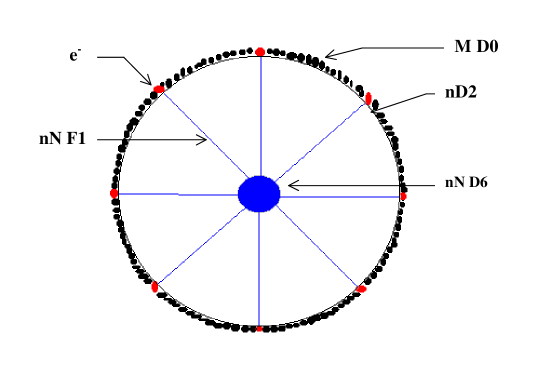
Figure 1: This figure represents a generalized fractional Quantum Hall Soliton describing the level $n$ of the hierarchy. It consists of $n$ coincident spherical D2 branes, $nN=\Sigma_{i=1}^{n}N_{i}$ fundamental strings and $M=\Sigma_{i=1}^{n}M_{i}$ D0 branes.

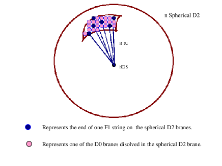
Figure 2: represents a portion of the $n$ coincident spheres describing the generalized fractional Quantum Hall Soliton.

Comments

The generalized quantum Hall soliton describes, amongst others, a set of $N_{1}+N_{2}+...+N_{n}$ particles. Upon taking all $N_{a}$’s equal to $N$, the system has then $nN$ particles and a richer symmetry which make it more or less simple to handle. We will consider hereafter this special case.
For finite $N_{a}$’s, F1 string ends $X^{i}(t)$ of the full set $\{NF1\}=\bigcup_{a=1}^{n}\{{N_{a}}F1\}$, with $nN$ particles, are valued in $Adj_{U(n)\otimes U(N)}$ with very particular coefficients. These coefficients are fixed by the nature of the $F1_{(a)}$ and $F1_{(b)}$ interactions which, for the case of Haldane hierarchy, should be in agreement with the two constraints imposed by the effective CS gauge model of the FQH systems.
String ends of the (${N_{a}}F1$) subsystem of $\{({N_{a}}F1)_{1\leq a\leq n}\}$, are described by the $N\times N$ matrix $X_{a}^{i}(t)$. This one dimensional field is just the development of $X^{i}(t)=\sum_{a=1}^{n}t^{a}X_{a}^{i}(t)$, where the $n$ $t^{a}$ hermitian matrices are given by a particular subset of the $u(n)$ algebra generator basis system. The $X^{i}(t)$ fields describe then the full set $\{({N_{a}}F1)_{1\leq a\leq n}\}$. Moreover according the analysis of section 3, it is more convenient to expand $X^{i}(t)$ as:

$$(X^{i}(t))_{\alpha\beta}=y^{i}\delta_{\alpha\beta}+\varepsilon^{ij}\ \ \Sigma_{a,b=1}^{n}\ \ [(A_{j}(t))_{\alpha\beta}^{a}\ \Gamma_{ab}\ (t^{b})],$$ (44)

where $\alpha,\beta=1,...,N$ and where $\Gamma$ is a $n\times n$ matrix whose entries $\Gamma_{ab}$ scale as $(length)^{2}$. $\Gamma$ generalizes just the one dimensional non commutative parameter involved in the analysis on the Laughlin state.
In the limit $N$ infinite, the F1 string ends fill all the space of the D2 branes and so the 1D $N\times N$ matrix $(A_{j})_{\alpha\beta}(t)$ is mapped to (2+1)D gauge field $A_{j}(t,y)$. Each set of ($N_{a}F1$) strings is then represented by a 2+1 dimensional gauge field $A^{(a)}_{\mu}$ and consequently the full F1 string ends set $\bigcup_{a=1}^{n}\{({N_{a}}F1)\}$ is described by the gauge field system $\{A^{(a)}_{\mu},1\leq a\leq n\}$. F1 string interactions are carried by the $K_{ab}$. Finally note that the D6 branes appear as external source of charge which couples to the CS gauge fields.

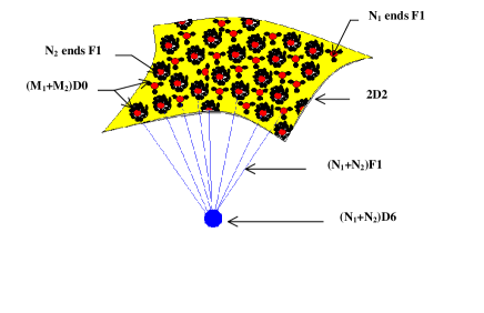
Figure 3: Here is represented the Haldane state of filling fraction $\nu=\frac{2}{5}$ realized as $\frac{1}{3}+\frac{1}{15}$. States with 3 D0 branes correspond to $\nu_{L}=\frac{1}{3}$ and those with 15 D0 branes for $\nu_{L}=\frac{1}{15}$.

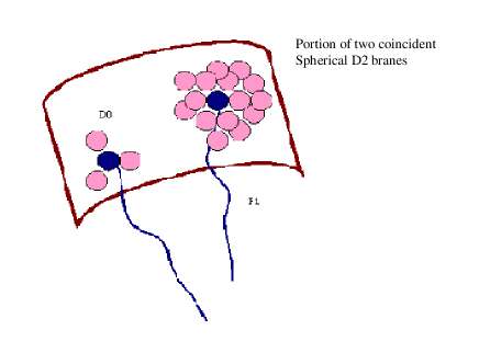
Figure 4: Here we show two F1 string ends of the level two of the hierarchy of filling fraction $\frac{2}{5}$ using the splitting $\frac{1}{3}+\frac{1}{15}$. The elementary $\frac{1}{3}$(resp $\frac{1}{15}$) state is represented as an F1 string end surrounded by 3 (resp 15) D0 branes.

5 More Results

Here we give the results for generic levels of the Haldane hierarchy by following the lines of section 3. In this case FQH hierarchical states at level $n$ are described, for a finite number $nN$ of particles, by a one dimensional $nN\times nN$ hermitian matrix $X^{i}(t)$ field valued in the $u(n)\oplus u(N)$ algebra. The corresponding matrix model for the strong $B$ regime reads as,

$$S=\frac{1}{g^{2}_{n}}\int dt\epsilon_{ij}Tr_{u(n)\oplus u(N)}[(\dot{X}+i[A_{0},X^{i}])X^{j}+\theta\epsilon^{ij}A_{0}],$$ (45)

where $g_{n}$ is a coupling constant. This action extends the Susskind model as well as the formula (20) respectively obtained by setting $n=1$ and $n=2$. Eq(45) defines then a sequence of models in one to one correspondence with FQH hierarchy. For a finite number $N$, the $X^{i}$’s may be treated as

$$X^{i}=[y^{i}+Z^{i}_{0}]I_{n}+\sum_{a=1}^{n^{2}-1}Z^{i}_{a}t^{a},$$ (46)

where $I_{n}$ is the $n\times n$ identity matrix, the $t^{a}$’s are the $(n^{2}-1)\ su(n)$ generators and where each component $Z^{i}_{a}$ is itself given by a $N\times N$ matrix of $AdjU(N)$. As we have noted in section 3, the $Z_{a}^{i}$ fluctuations around the classical configuration are not all of them allowed in the study of FQH hierarchy; only $n$ amongst the $n^{2}$ ones are involved in the effective CS model as shown on eq(1). To get the right fluctuations, we shall follow the method we developed previously by introducing a new vector basis $\{\tau^{a};\ 1\leq a\leq n^{2}\}$ of the $u(n)$ algebra. This new basis is related to the old one as

$$\tau^{a}=\Gamma^{a}_{b}\ t^{b}\ \ ,$$ (47)

where $\Gamma^{a}_{b}$ is an invertible $n\times n$ matrix. Note that as far as this change is concerned, we will need in practice only $n$ matrices $\tau^{a}$, $1\leq a\leq n$ which, without loss of generality, can be taken as:

$$\tau_{1} = [\gamma_{1}I+(\delta_{1}E_{1}^{+}+\bar{\delta}_{1}E_{1}^{-})],$$

$$\tau_{a} = [-(\beta_{a}E_{a-1}^{+}+\bar{\beta}_{a}E_{a-1}^{-})+\gamma_{a}H_{a-1}+(\delta_{a}E_{a}^{+}+\bar{\delta}_{a}E_{a}^{-})],\ \ 2\leq a\leq n-1,$$

$$\tau_{n} = [-(\beta_{n}E_{n-1}^{+}+\bar{\beta}_{n}E_{n-1}^{-})+\gamma_{n}H_{n-1}].$$ (48)

In this equation the $H_{a}$’s and $E_{a}^{\pm}$’s are respectively the $n\times n$ matrix Cartan generators and Chevalley step operators of the $su(n)$ algebra while the $\beta_{a}$’s , $\gamma_{a}$’s and $\delta_{a}$’s are parameters which should be related to the order parameters of $SLn$. The $E_{a}^{\pm}$’s are the generators associated with the $\alpha_{a}$ simple roots of the $su(n)$ algebra. Notice that the above expression for the $\tau_{a}$ matrices depend on $5n-4$ real moduli; that is $n$ real parameters $\gamma_{1},\gamma_{2},...,\gamma_{n}$, $n-1$ complex $\beta_{2},...,\beta_{n}$ and $n-1$ complex $\delta_{1},...,\delta_{n-1}$. These moduli are not all of them independent; only a subset of them do. Later on we will show that for the case of Haldane hierarchy there are $n+1$ independent moduli giving the $n$ CS levels $l_{a}$ and the non commutativity parameter $\theta$.

In the limit $N$ infinite, the 1D $u(n)\oplus u(N)\ Z^{i}(t)$ fields are mapped to (2+1)dimensional $\ Z^{i}(t,y^{1},y^{2})$ valued in the $u(n)$ algebra which in turns can be set as $Z^{i}(y)=\varepsilon^{ij}A_{j}(y)$ as required by the $U(\infty)\sim SDiff(R^{2})$ invariance. Taking into account all above features and following the same lines we used for the $SL2$ mode we get after some algebra,

$$S=\frac{1}{g^{2}_{n}}\int d^{3}y\epsilon^{\mu\nu\rho}Tr_{U(n)}[\partial_{\mu}A_{\nu}A_{\rho}-\frac{i}{3}A_{\mu}\{A_{\nu},A_{\rho}\}]+0(2).$$ (49)

Moreover, as we noted in the case of level two of the hierarchy, the expansion (49) is not the one needed to describe the FQH hierarchy; it involves $n^{2}$ gauge variables while we need $n$ fields only. This means that eq(46) should be constrained as in eq (44).

For the $n-th$ level of the Haldane hierarchy, the SLn constraint eqs leading to the appropriate result read as:

$$A_{i}(y) = \sum_{a=1}^{n}\tau_{a}A^{a}_{i}(y),$$ (50)

$$Tr(\tau_{a}\tau_{b})-\frac{l_{a}}{g_{n}^{2}}\ \delta_{ab} \neq 0\ \ for\ \ b={a\pm 1},$$ (51)

$$Tr(\tau_{a}\tau_{b})-\frac{l_{a}}{g_{n}^{2}}\ \delta_{ab} = 0\ \ otherwise.$$

The $\tau_{a}$ solutions of (51) are indeed given by eqs(48). Putting these constraint eqs back into the above action, we get similar relations to those given by eqs(33); but describe now generic $n-th$ levels of the Haldane hierarchy.

$$K_{ab} = \frac{1}{g^{2}_{n}}Tr(\tau_{a}\tau_{b})\ \ \ \ \ (a)$$

$$C_{abc} = \frac{1}{g^{2}_{n}}Tr(\tau_{a}\tau_{b}\tau_{c})\ \ \ \ (b)$$ (52)

These formulas are then valid for any order $n$ of the hierarchy and are, in this sense, universal. Furthermore, using the explicit form of the $K$ matrix of Haldane namely,

$$K_{ab}=l_{a}\delta_{a,b}-\delta_{a,b-1}-\delta_{a,b+1},$$ (53)

we can determine the link between the $\beta_{a}$ , $\gamma_{a}$ and $\delta_{a}$ parameters appearing in eqs(48) and the $l_{a}$ order parameters. We have,

$$g_{n}^{2} = (\delta_{a}\bar{\beta}_{a}+\bar{\delta}_{a}\beta_{a}),$$

$$g_{n}^{2}l_{1} = (n\gamma_{1}^{2}+2\delta_{1}\bar{\delta}_{1}),$$

$$g_{n}^{2}l_{a} = 2(\gamma_{a}^{2}+\beta_{a}\bar{\beta}_{a}+\delta_{a}\bar{\delta}_{a}),$$ (54)

$$g_{n}^{2}l_{n} = 2(\gamma_{n}^{2}+\beta_{n}\bar{\beta}_{n}).$$

Since Haldane hierarchical states are specified by the $l_{a}$ levels of the CS gauge model and the $\theta$ parameter, the $\beta_{a}$ and $\gamma_{a}$ moduli should be constrained. A convenient choice for the $\beta_{a}$ and $\gamma_{a}$ parameters consists of setting set $\beta_{a}=\delta_{a}=\beta$, for all values of $a$. This permits to have the right degrees of freedom one has in Haldane theory; that is: $\gamma_{1},\gamma_{2},...,\gamma_{n}$ and $\beta$. Therefore the $\tau_{a}$ matrices of eqs (48) are reduced to:

$$\tau_{1} = {\gamma_{1}}I+\beta\ (E_{1}^{+}+E_{1}^{-}),$$

$$\tau_{a} = {\gamma_{a}}H_{a-1}-\beta\ (E_{a-1}^{+}+E_{a-1}^{-}+E_{a}^{+}+E_{a}^{-}),\ \ 2\leq a\leq n-1,$$

$$\tau_{n} = {\gamma_{n}}H_{n-1}-\beta\ (E_{n-1}^{+}+E_{n-1}^{-}).$$ (55)

and so eqs(54) is reduced to

$$g_{n}^{2} = 2\beta^{2},$$

$$g_{n}^{2}l_{1} = (n\gamma_{1}^{2}+2\beta^{2}),$$

$$g_{n}^{2}l_{a} = 2(\gamma_{a}^{2}+2\beta^{2}),$$ (56)

$$g_{n}^{2}l_{n} = 2(\gamma_{n}^{2}+\beta^{2}).$$

These eqs may be rewritten in the following equivalent form which establishes the link between the CS integers $l_{1},l_{2},l_{n}$ and the coupling $g_{n}$ on one hand and the $\beta$ and $\gamma_{a}$ moduli on the other hand;

$$l_{1} = (1+{n\gamma_{1}^{2}\over g_{n}^{2}})^{\frac{1}{2}}\ \ \ \ \ odd\ integer,$$

$$l_{a} = 2(1+{\gamma_{a}^{2}\over g_{n}^{2}})^{\frac{1}{2}}\ \ \ \ \ even\ integer;\ \ 2\leq a\leq n-1,$$

$$l_{n} = (1+{2\gamma_{n}^{2}\over g_{n}^{2}})^{\frac{1}{2}}\ \ \ \ \ even\ integer.$$ (57)

Actually the above eqs constitute a generalization of the Susskind result on Laughlin state and the level 2 Haldane state we have obtained in section 3, eqs(38). These analysis correspond just the two leading modes $SL1$ and $SL2$ of a hierarchy of $SLn$ configurations.

6 Conclusion

In this paper we have developed the non commutative Chern-Simons gauge analysis for the description of the hierarchical states of fractional quantum Hall liquids. For a generic level $n$ of the hierarchy, we have shown that Susskind analysis made for the Laughlin state is naturally generalization for the hierarchical one. Using general features on the CS effective field model of FQH hierarchical states, we have first studied hierarchical states at level two with a special focus on the Haldane hierarchy and then considered the generic case. Among our results:

(a) The derivation of the matrix model describing a set of a finite number $nN$ of FQH particles which reads as:

$$S=\frac{1}{g^{2}_{n}}\int dt\ \epsilon_{ij}\ Tr_{u(n)\oplus u(N)}[(\dot{X}+i[A_{0},X^{i}])X^{j}+\theta\epsilon^{ij}A_{0}],$$ (58)

where the various quantities appearing in this action were introduced in the core of this paper. Notice that for $n=1$, this action coincides with that given in [1] and further elaborated in [32] in connection with the study of edge excitations.

(b) The obtention of the generalized mapping, extending the Susskind change $X^{i}=y^{i}+\theta\varepsilon^{ij}\ A_{j}(y)$ made for the Laughlin state, is given by the following $n\times n$ matrix:

$$(X^{i}_{BD})=\left(\matrix{X^{i}_{11}&X^{i}_{12}&...&X^{i}_{1n}\cr X^{i}_{21}&X^{i}_{22}&...&X^{i}_{2n}\cr.&.&...&.\cr.&.&...&.\cr X^{i}_{n1}&X^{i}_{n2}&...&X^{i}_{nn}}\right)$$ (59)

where

$$X^{i}_{BD}=y^{i}\delta_{BD}+\theta\varepsilon^{ij}(\sum_{a=1}^{n}A^{a}_{j}(y)\ (\tau_{a})_{BD}),$$ (60)

and where the $\tau_{a}$’s are as in eqs(55-57). Putting eq(60) back into eq(58), one gets the well known effective field action (1), but also corrections induced by $(2+1)$ space-time non commutativity as shown in eq(49).

(c) the proof that the $K_{ab}$ order parameters are indeed related to the non commutativity $\theta$ parameter; they are given by $\theta^{-2}Tr(\tau_{a}\tau_{b})$, where the   $\{\tau_{a},1\leq a\leq n\}$ set is given by a specific system of $n\times n$ matrices depending on $n+1$ moduli $\gamma_{1},...,\gamma_{n}$ in addition to the coupling constants $g_{n}$. The $\gamma_{a}$ moduli are shown to be related to the $l_{a}$ integers of the FQH Chern-Simons effective field theory. These relations were worked out explicitly for the case of Haldane hierarchy as shown in eqs (57).

(d) our analysis predicts moreover the existence of a tensor $C_{abc}$ of induced order parameters. This set of order parameters is shown however to be not a new class as these orders are not really independent. The $C_{abc}$’s are shown to be given by $\theta^{-2}Tr(\tau_{a}\tau_{b}\tau_{c})\propto\theta d_{abc}$, where $d_{abc}$ are numbers expressed in terms of the $u(n)$ Chevalley generators $H_{a},E_{a}^{+},E_{a}^{-}$.

Furthermore, we have studied the link between Hierarchical states of FQH fluids and D branes. By extending the construction of refs [2,3] associated with the Laughlin state, we have built the generalized quantum Hall soliton supposed to describe generic SLn modes; $n\geq 2$, as a subsystem. As in the case of the Laughlin state, the generalized quantum Hall soliton carries here also much more physics; in particular two coupled CS gauge theories, one describing the electron fluid and the other the fluid of D0 branes. In the present analysis we have considered the special situation where all $N_{a}$’s are equal. We have supposed that the number $N_{a}$ of particles one obtains from the $a$-th condensation is equal to $N$ for any index $a$. The resulting system has a total number of particles equal to $N_{1}+N_{2}+...+N_{n}=nN$ and a $U(n)$ symmetry. It would be interesting to explore the general issue for a system of finite number of particles where the $N_{a}$’s are different and rebuild the underlying effective non commutative CS gauge model.

Acknowledgements
This project has been supported by the SARS/99 programme, Rabat University.

References

1. ]  Leonard Susskind, The Quantum Hall fluid and Noncommutative Chern-Simons Theory. hep-th/0101029.

2. ] C. Duval, P. A.Horv thy ,Exotic galilean symmetry in the non-commutative plane, and the Hall effect, hep-th/0106089

3. ] Bogdan Morariu, Alexios P. Polychronakos, Finite Noncommutative Chern-Simons with a Wilson Line and the Quantum Hall Effect, hep-th/0106072

4. ] Alexios P. Polychronakos, Quantum Hall states on the cylinder as unitary matrix Chern-Simons theory, hep-th/0106011

5. ] Simeon Hellerman, Mark Van Raamsdonk, Quantum Hall Physics = Noncommutative Field Theory ,hep-th/0103179 Noncommutative Chern-Simons Solitons

6. ] Dongsu Bak, Sung Ku Kim, Kwang-Sup Soh, Jae Hyung Yee Phys.Rev. D64 (2001) 025018

7. ]  John H. Brodie (SLAC), L. Susskind, N. Toumbas, How Bob Laughlin Tamed The Giant Graviton From TAUB - NUT SPACE, JHEP 0102:003,2001 and hep-th/0010105

8. ]  Steven S. Gubser, Mukund Rangamani,D-Brane Dynamics and the Qunatum Hall Effect. JHEP 0105:041,2001; hep-th/0012155

9. ] Simeon Hellerman, Leonard Susskind; Realizing the Quantum Hall System in String Theory,hep-th/0107200

10. ] O. Bergman, J. Brodie, Y. Okawa;The Stringy Quantum Hall Fluid, hep-th/0107178

11. ] Avinash Khare, M. B.Paranjape, JHEP 0104 (2001) 002

12. ]  R.B.Laughlin, Phys.rev.Lett. 50(1983)1395.
    E.Fradkin, Field Theories of Condensed Matter Systems, Lecture Note Series V82(1991)

13. ]  X.G. Wen and A. Zee ,Phys.Rev.B46(1992)2290.
    Xiao-Gang Wen, Topological Orders and Edge Excitations in FQH States. PRINT-95-148 (MIT),cond-mat/9506066.

14. ]  R.B. Laughlin, Anomalous Quantum Hall Effect: An Incompressible Quantum Fluid with Fractionally Charged Excitations. Phys.Rev.Lett.50:1395,1398
    D.arovas, J.R.Schrieffer,F.Wilczek: Fractional Statistics in the Quantum Hall Effect,Phys.Rev.Lett.53(1984)722-723

15. ]  Safi Bahcall and Leonard Susskind , Fluid Dynamics, Chern-Simons Theory and the Quantum Hall Effect; Int.J.Mod.Phys.B5:2735-2750,1991 35

16. ]  X.G. Wen and A. Zee Phys.Rev.B46:2290-2301,1992; B.Blok and X.G Wen Phys.Rev.B43:8337,1991, Phys.Rev.B42:8145-8156,1990; ibid 8133-8144,1990.
    A.Jellal Int.J.Theor.Phys.37:2751-2755,1998

17. ]  J. Frohlich and A. Zee, Nucl.Phys.B364:517-540,1991; Jurg Frohlich, Thomas Kerler and Emmanuel Thiran; Structure the set of Incompressible Quantum Hall Fluids.Nucl.Phys.B453:670-704,1995.

18. ] N.Read,Phys.Rev.Lett. 65,(1990)1502.

19. ] B.Blok and X.G.Wen, Phys.Rev. B42,(1990)8133-8145.

20. ] R.E.Prange and S.M. Girvin, The Quantum Hall effect(Springer, New York, 1987).

21. ] F.D.M. Haldane, Fractional Quantization of the Hall Effect: A Hierarchy of Incompressible Quantum Fluid States. Phys.Rev.Lett.51:605-608,1983

22. ] Eduardo Fradkin, Lecture Note Series 82 (Field Theories of Condensed matter systems) 1991.

23. ] Steven M. Girvin,(Indiana University), ”The Quantum Hall Effect: Novel Excitations and Broken Symmetries”,cond-mat/9907002.

24. ] S.Hellerman and L.Susskind:Realizing the Quantum Hall System in String Theory, hep-th/0107200.

25. ] I. Benkaddour, A. EL Rhalami, E.H. Saidi :Fractional Quantum Hall Excitations as RdTS Highest Weight State, hep-th/0101188.

26. ] H.B.Geyer(Ed):Field Theory, Topology and Condensed matter Physics,Proceedings of the Ninth Chris Engelbrecht Summer School in theoretical Physics. Held at:Storms River Mouth, Tsitsikamma National Parkc, South africa, 17-28 January 1994.Springer 1995. (see) A.Zee,Quatum Hall Fluid

27. ] B.Halprin: Statistics of Quasiparticles and the hierarchy of fractional Quantum Hall States, Phys.Rev.Lett.52(1984)1583-1586.

28. ] N.Read, Excitation Structure of the Hierarchy Scheme for the fractional Quantum Hall effect, Phys.Rev.Lett.65(1990)1502-1505.

29. ] N.Seiberg and E.Witten, JHEP 9909:032,1999, hep-th/9908142

30. ] M .Olshanetsky and A.M.Perelomov, Phys.Rept.71(1981)313 and 94(1983)6
    F.Calogero, J.Math.Phys.12,419(1971)
    A.P.Polychronakos,Phys.Lett.B 266,29 (1991)

31. ] J.Polchinski, String theory, Cambridge Univ Press 1998.

32. ] A.P. Polychronakos: Quantum Hall states as matrix Chern-Simons theory, JHEP 0104 (2001) 011,hep-th/0103013.