hep-th/0108090

UFIFT-HEP-01-12

CRETE-01-11

Pair creation and axial anomaly in light-cone $QED_{2}$

T. N. Tomaras^† and N. C. Tsamis^‡

Department of Physics and Institute of Plasma Physics
University of Crete and FO.R.T.H.
P.O.Box 2208, 710 03 Heraklion, Crete; GREECE.

R. P. Woodard^∗

Department of Physics, University of Florida
Gainesville, FL 32611; UNITED STATES.

ABSTRACT

The 1+1 dimensional massive Dirac equation is solved exactly in light-cone coordinates for $x^{+}>0$ and $x^{-}>-L$, in the presence of an arbitrary $x^{+}$ dependent electric field. Our solution resolves the ambiguity at $p^{+}=0$. We also obtain the one loop rate for pair production for a positive electric field, compute the expectation values of the vector and axial vector currents, and recover the well known anomaly $e^{2}E/\pi$ in the divergence of the latter. A final intriguing result is that the theory seems to exhibit a phase transition in the limit of infinite $L$.

PACS numbers: 11.15.Kc, 12.20-m

^† e-mail: tomaras@physics.uoc.gr

^‡ e-mail: tsamis@physics.uoc.gr

^∗ e-mail: woodard@phys.ufl.edu

1 Introduction

The phenomenon of electron-positron pair production in an external electric field has already a long history. What happens initially when a prepared state is released in the presence of a homogeneous electric field is that electron-positron pairs emerge from the vacuum to form a current which diminishes the electric field. If the state is released on a surface of constant $x^{0}$ with no initial charge then the electric field at later times depends only upon $x^{0}$. This process was considered long before the ultraviolet problem of quantum electrodynamics was resolved [1, 2, 3]. Schwinger invented what we now know as the in-out background field effective action to compute the rate of particle production per unit volume in the presence of a strictly constant electric field [4]. Since then a variety of articles [5]–[12] and monographs [13, 14] have treated the issue of what happens when the effect becomes strong.

In the light-cone analog to this process a source-free state is released on a surface of constant $x^{+}\equiv(x^{0}+x^{1})/\sqrt{2}$ in the presence of a homogeneous electric field which is parallel to $x^{1}$. The resulting evolution yields a homogeneous electric field which depends upon $x^{+}$ rather than $x^{0}$, and has potentially interesting applications in the study of the onset and evolution of electric fields in the vicinity of a star formed by the collapse of charged matter [16]. An amazing feature of Dirac theory in any such $x^{+}$ dependent background is that the mode functions are simple [15]. This fact had been noted previously for the special case of a constant electric field [17, 18, 19], although without resolving the ambiguity at $p^{+}=0$. By allowing the electric field to depend arbitrarily upon $x^{+}$ it is for the first time possible to study back-reaction analytically in the presence of a class of backgrounds which is guaranteed to include the actual solution.

A crucial insight in resolving the ambiguity at $p^{+}=0$ was that the light-cone evolution problem is not well posed with only initial value data from the surface at $x^{+}=0$ [15]. One must also provide data on a surface of constant $x^{-}\equiv(x^{0}-x^{1})/\sqrt{2}$, which we took to be $x^{-}=-L$. Incidentally, this fact has been noted before in [20], while an early attempt to analyze its consequences in the quantum theory of massless fermions, may be found in [21]. Although correct, our previous solution for the electron field operator was only valid in the distributional limit of $L\longrightarrow\infty$. This restricted its to use to expectation values of nonsingular operators such as $J^{+}$, but prevented us from evaluating operators such as $J^{-}$ which diverge as $L$ goes to infinity. In the present work we remove this restriction by deriving an exact operator solution which is valid for all $L$. The result is a vast increase in the range of applications which we will exploit in a number of ways for the special case of 1+1-dimensional, massive quantum electrodynamics ($QED_{2}$). Note, however, that the exact operator solution is valid for any spacetime dimension, as well as for zero mass.

This paper contains seven sections of which this introduction is the first. Section 2 begins by giving our light-cone coordinate and gauge conventions, which we have converted from those of our initial treatment [15] to standard notation. This section also presents the complete operator solution for Dirac theory in the presence of an arbitrary $x^{+}$ dependent electric field background, expressed in terms of the field operators on the surfaces of $x_{+}=0$ and $x_{-}=-L$. Section 3 gives the quantum operator algebra and the conditions which define the initial, source-free state. We use these results in Section 4 to give an explicit, analytic derivation for the probability of particle production in our general background. In Section 5 we compute the one loop expectation value of the vector current operator and show that it is conserved. The fact that our results depend non-analytically upon the background field in the large $L$ limit seems to indicate that we are seeing an infinite volume phase transition. In Section 6 we compute the one loop expectation values of the axial currents and of the pseudoscalar bilinear. We exploit these results to derive the standard formula for the axial vector anomaly for the first time ever on the light-cone with $m\neq 0$. Section 7 gives our conclusions and some comments about the subtle limiting procedure required for computing back-reaction.

2 The model and its solution

The massive Schwinger model is defined by the Lagrangian density,

$${\cal L}=\overline{\Psi}i\gamma^{\mu}(\partial_{\mu}+ieA_{\mu})\Psi-m\overline{\Psi}\Psi-{1\over 4}F_{\mu\nu}F^{\mu\nu}\;,$$ (1)

with $\mu,\nu=0,1$. $A_{\mu}$ is the gauge potential and $\Psi$ is the fermion Dirac doublet field. The electromagnetic coupling constant is $e<0$. Our conventions for the flat spacetime metric, and the Gamma matrices are the ones used by Bjorken and Drell [24], appropriately reduced to two spacetime dimensions. Thus, $\eta_{\mu\nu}=(+1,-1)$, $\{\gamma_{\mu},\gamma_{\nu}\}=2\eta_{\mu\nu}$, $\gamma^{0}{\gamma^{\mu}}^{\dagger}\gamma^{0}=\gamma^{\mu}$, ${\gamma_{5}}^{\dagger}=\gamma_{5}$.

We shall adhere to the standard light-cone conventions [25] for defining coordinates, $x^{\pm}\equiv{1\over{\sqrt{2}}}(x^{0}\pm x^{1})$. Identical formulae relate the light-cone components of an arbitrary vector $V^{\mu}$ to the Cartesian ones. In these coordinates the inner product of two vectors is $a^{\mu}b_{\mu}=a^{0}b^{0}-a^{1}b^{1}=a^{+}b^{-}+a^{-}b^{+}$. The non-vanishing components of the metric are $g_{+-}=g_{-+}=1$, and consequently for any vector one has $a_{+}=a^{-},a_{-}=a^{+}$. With the standard definition $\partial_{\pm}\equiv\partial/\partial x^{\pm}$, one obtains $\partial_{\mu}V^{\mu}=\partial_{+}V^{+}+\partial_{-}V^{-}$ for any vector field $V^{\mu}$.

We define the light-cone spinor projection operators by ${\cal P}_{\pm}\equiv{1\over 2}(I\pm\gamma^{0}\gamma^{1})={1\over 2}(I\pm\gamma_{5})={1\over 2}\gamma^{\mp}\gamma^{\pm}$. In direct analogy with all other vectors $\gamma^{\pm}\equiv{1\over{\sqrt{2}}}(\gamma^{0}\pm\gamma^{1})$. They satisfy $(\gamma^{\pm})^{2}=0$ and $\{\gamma^{+},\gamma^{-}\}=2$. The Dirac spinor decomposes into $\Psi=\psi_{+}+\psi_{-}$, with $\psi_{\pm}\equiv{\cal P}_{\pm}\Psi$. Finally, note that in 1+1 dimensions ${\rm Tr}{\cal P}_{\pm}=1$.

A convenient representation of the Dirac matrices is $\gamma^{0}=\sigma_{1}$, $\gamma^{1}=i\sigma_{2}$. In this representation $\gamma_{5}=\gamma^{0}\gamma^{1}=-\sigma_{3}$, while ${\cal P}_{+}={\rm diag}(0,1)$ and ${\cal P}_{-}={\rm diag}(1,0)$. However, we shall work in a representation independent way.

We shall here go over the relevant bilinears without attention to either operator ordering or to regularization. These issues will be fully addressed in Sections 5 and 6. The light-cone components $J^{\pm}\equiv{1\over{\sqrt{2}}}(J^{0}\pm J^{1})$ of the electromagnetic current $J^{\mu}=e\overline{\Psi}\gamma^{\mu}\Psi$ are,

$$J^{\pm}=\sqrt{2}e\psi_{\pm}^{\dagger}\psi_{\pm}\;.$$ (2)

Similarly, the light-cone components $J_{5}^{\pm}\equiv{1\over{\sqrt{2}}}(J_{5}^{0}\pm J_{5}^{1})$ of the axial current $J_{5}^{\mu}=\overline{\Psi}\gamma^{\mu}\gamma_{5}\Psi$ take the form,

$$J_{5}^{\pm}=\pm\sqrt{2}\psi_{\pm}^{\dagger}\psi_{\pm}=\pm J^{\pm}/e\;.$$ (3)

Finally, the bilinear $J_{5}\equiv\overline{\Psi}\gamma_{5}\Psi$ in terms of $\psi_{\pm}$ becomes,

$$J_{5}={1\over\sqrt{2}}(\psi_{-}^{\dagger}\gamma^{+}\psi_{+}-\psi_{+}^{\dagger}\gamma^{-}\psi_{-})\;.$$ (4)

We fix the gauge by setting $A_{+}=0$ with the initial value of $A_{-}$ also zero,

$$A_{-}(x^{+})=-\int_{0}^{x^{+}}duE(u)\;.$$ (5)

The Dirac equation in an arbitrary $A_{-}(x^{+})$ background field takes the form:

$$\left(\gamma^{+}i\partial_{+}+\gamma^{-}(i\partial_{-}-eA_{-})-m\right)\Psi=0.$$ (6)

It implies the conservation of the electromagnetic current

$$\partial_{+}J^{+}+\partial_{-}J^{-}=0\;,$$ (7)

as well as the following relation between $J_{5}$ and the divergence of the axial vector current,

$$e\partial_{\mu}J_{5}^{\mu}-2iemJ_{5}=2\partial_{+}J^{+}-2iemJ_{5}=0\;.$$ (8)

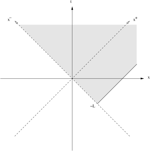
Figure 1: The domain (shaded) of our solution for $\psi_{\pm}(x^{+},x^{-})$. We specify the initial values of $\psi_{+}(0,x^{-})$ for all $x^{-}>-L$ and of $\psi_{-}(x^{+},-L)$ for all $x^{+}>0$.

Multiplying (6) by $\gamma^{+}$ and $\gamma^{-}$ respectively, one may rewrite it in the equivalent form of the system of equations,

$$i\partial_{+}\psi_{+} = {m\over 2}\gamma^{-}\psi_{-}\;,$$ (9)

$$(i\partial_{-}-eA_{-})\psi_{-} = {m\over 2}\gamma^{+}\psi_{+}\;.$$ (10)

Equations (9) and (10) can be integrated,

$$\psi_{+}(x^{+},x^{-}) = \psi_{+}(0,x^{-})-{{im}\over 2}\int_{0}^{x^{+}}du\gamma^{-}\psi_{-}(u,x^{-})\;,$$ (11)

$$\psi_{-}(x^{+},x^{-}) = e^{-ieA_{-}(x^{+})(x^{-}+L)}\psi_{-}(x^{+},-L)$$ (12)

$$\qquad-{{im}\over 2}\int_{-L}^{x^{-}}dve^{-ieA_{-}(x^{+})(x^{-}-v)}\gamma^{+}\psi_{+}(x^{+},v)\;,$$

to express $\psi_{\pm}(x^{+},x^{-})$ in terms of initial data $\psi_{+}(x^{+}=0,x^{-}>-L)$ and $\psi_{-}(x^{+}>0,x^{-}=-L)$ on the semi-axes shown in Fig. 1. Substituting (12) into (11) and iterating, one is led to the following infinite series solution for $\psi_{+}$,

$$\psi_{+}(x^{+},x^{-})=\sum_{n=0}^{\infty}\Bigl{(}-{{m^{2}}\over 2}\Bigr{)}^{n}\int_{0}^{x^{+}}du_{1}\int_{-L}^{x^{-}}dv_{1}e^{-ieA_{-}(u_{1})(x^{-}-v_{1})}\int_{0}^{u_{1}}du_{2}$$ (13)

$$\int_{-L}^{v_{1}}dv_{2}e^{-ieA_{-}(u_{2})(v_{1}-v_{2})}\cdots\int_{0}^{u_{n-1}}du_{n}\int_{-L}^{v_{n-1}}dv_{n}e^{-ieA_{-}(u_{n})(v_{n-1}-v_{n})}$$

$$\hskip 56.9055pt\times\Biggl{\{}\psi_{+}(0,v_{n})-i{m\over 2}\gamma^{-}\int_{0}^{u_{n}}due^{-ieA_{-}(u)(v_{n}+L)}\psi_{-}(u,-L)\Biggr{\}}.\quad$$

One next introduces the identity,

$$\int_{-L}^{v_{n-1}}dv_{n}e^{-ieA_{-}(v_{n-1}-v_{n})}=\int_{-L}^{\infty}dv_{n}\int_{-\infty}^{\infty}{{dk^{+}}\over{2\pi}}{{ie^{-i(k^{+}+i/L)(v_{n-1}-v_{n})}}\over{k^{+}-eA_{-}(u_{n})+i/L}}\;,$$ (14)

sets $v_{n}=v$ and interchanges the order of integration to get,

$$\psi_{+}(x^{+},x^{-})=\int_{-L}^{\infty}dv\int_{-\infty}^{\infty}{dk^{+}\over 2\pi}e^{i(k^{+}+i/L)v}\sum_{n=0}^{\infty}\Bigl{(}-{{m^{2}}\over 2}\Bigr{)}^{n}\int_{0}^{x^{+}}du_{1}\int_{-L}^{x^{-}}dv_{1}$$ (15)

$$\times e^{-ieA_{-}(u_{1})(x^{-}-v_{1})}\cdots\int_{0}^{u_{n-3}}du_{n-2}\int_{-L}^{v_{n-3}}dv_{n-2}e^{-ieA_{-}(u_{n-2})(v_{n-3}-v_{n-2})}$$

$$\qquad\times\int_{0}^{u_{n-2}}du_{n-1}\int_{-L}^{v_{n-2}}dv_{n-1}e^{-ieA_{-}(u_{n-1})(v_{n-2}-v_{n-1})}e^{-i(k^{+}+i/L)v_{n-1}}$$

$$\qquad\qquad\times\int_{0}^{u_{n-1}}{idu_{n}\over{k^{+}-eA_{-}(u_{n})+i/L}}\Biggl{\{}\psi_{+}(0,v)$$

$$\hskip 113.81102pt-i{m\over 2}\gamma^{-}\int_{0}^{u_{n}}due^{-ieA_{-}(u)(v+L)}\psi_{-}(u,-L)\Biggr{\}}\;.\qquad$$

This is the key step at which we deviate from our previous solution [15]. In particular it will not be necessary, proceeding this way, to take $L$ to infinity.

The integration over $v_{n-1}$ gives,

$$\int_{-L}^{v_{n-2}}dv_{n-1}e^{-ieA_{-}(u_{n-1})(v_{n-2}-v_{n-1})}e^{-i(k^{+}+i/L)v_{n-1}}$$ (16)

$$\qquad={ie^{-i(k^{+}+i/L)v_{n-2}}-ie^{-ieA_{-}(u_{n-1})(L+v_{n-2})}e^{i(k^{+}+i/L)L}\over k^{+}-eA_{-}(u_{n-1})+i/L}\;.$$

Note that the second term in (16) gives zero inside the $k^{+}$ integral. This is because $(v+L)$ is positive in the range over which $v$ is integrated, so we can close the contour of the $k^{+}$ integral above. The result must be zero because the integrand is analytic in the upper half plane.

Upon substitution of (16) our solution for $\psi_{+}$ becomes,

$$\psi_{+}(x^{+},x^{-})=\int_{-L}^{\infty}dv\int_{-\infty}^{+\infty}{{dk^{+}}\over{2\pi}}e^{i(k^{+}+i/L)v}\sum_{n=0}^{\infty}\Bigl{(}-{{m^{2}}\over 2}\Bigr{)}^{n}\int_{0}^{x^{+}}du_{1}\dots$$ (17)

$$\cdots\int_{0}^{u_{n-3}}du_{n-2}\int_{-L}^{v_{n-3}}dv_{n-2}e^{-ieA_{-}(u_{n-2})(v_{n-3}-v_{n-2})}e^{-i(k^{+}+i/L)v_{n-2}}$$

$$\qquad\times\int_{0}^{u_{n-2}}{idu_{n-1}\over{k^{+}-eA_{-}(u_{n-1})+i/L}}\int_{0}^{u_{n-1}}{idu_{n}\over{k^{+}-eA_{-}(u_{n})+i/L}}$$

$$\hskip 56.9055pt\times\Biggl{\{}\psi_{+}(0,v)-i{m\over 2}\gamma^{-}\int_{0}^{u_{n}}due^{-ieA_{-}(u)(v+L)}\psi_{-}(u,-L)\Biggr{\}}\;.\qquad$$

Then perform the $v_{n-2}$ integration, just like (16), and discard the lower limit as before. In this way all the $v_{i}$ integrations can be done to give,

$$\psi_{+}(x^{+},x^{-})=\int_{-L}^{\infty}dv\int_{-\infty}^{+\infty}{dk^{+}\over 2\pi}e^{i(k^{+}+i/L)(v-x^{-})}$$ (18)

$$\times\sum_{n=0}^{\infty}\int_{0}^{x^{+}}{-im^{2}/2\;du_{1}\over k^{+}-eA_{-}(u_{1})+i/L}\cdots\int_{0}^{u_{n-1}}{{-im^{2}/2\;du_{n}}\over{k^{+}-eA_{-}(u_{n})+i/L}}$$

$$\hskip 56.9055pt\times\Biggl{\{}\psi_{+}(0,v)-{i\over 2}m\gamma^{-}\int_{0}^{u_{n}}due^{-ieA_{-}(u)(v+L)}\psi_{-}(u,-L)\Biggr{\}}\;.\quad$$

Use of the identities,

$$\int_{0}^{x^{+}}du_{1}f(u_{1})\int_{0}^{u_{1}}du_{2}f(u_{2})\cdots\int_{0}^{u_{n-1}}du_{n}f(u_{n})={1\over n!}\Biggl{[}\int_{0}^{x^{+}}dyf(y)\Biggr{]}^{n}\;,$$ (19)

$$\int_{0}^{x^{+}}du_{1}f(u_{1})\cdots\int_{0}^{u_{n-1}}du_{n}f(u_{n})\int_{0}^{u_{n}}dug(u)$$ (20)

$$\hskip 113.81102pt=\int_{0}^{x^{+}}dug(u){1\over{n!}}\Biggl{[}\int_{u}^{x^{+}}dyf(y)\Biggr{]}^{n}\;,$$

leads to the final expression for $\psi_{+}$,

$$\psi_{+}(x^{+},x^{-})=\int_{-L}^{\infty}dv\int_{-\infty}^{+\infty}{{dk^{+}}\over{2\pi}}e^{i(k^{+}+i/L)(v-x^{-})}\Biggl{\{}{\cal E}[eA_{-}](0,x^{+};k^{+})\psi_{+}(0,v)$$ (21)

$$\hskip 28.45274pt-{i\over 2}m\gamma^{-}\int_{0}^{x^{+}}due^{-ieA_{-}(u)(v+L)}{\cal E}[eA_{-}](u,x^{+};k^{+})\psi_{-}(u,-L)\Biggr{\}}\;.\quad$$

The functional ${\cal E}[eA_{-}]$ is,

$${\cal E}[eA_{-}](u,x^{+};k^{+})\equiv\exp\Biggl{[}-{i\over 2}m^{2}\int_{u}^{x^{+}}{{du^{\prime}}\over{k^{+}-eA_{-}(u^{\prime})+i/L}}\Biggr{]}\;.$$ (22)

As for $\psi_{-}(x^{+},x^{-})$, it is obtained trivially from (9),

$$\psi_{-}(x^{+},x^{-})={1\over m}\gamma^{+}i\partial_{+}\psi_{+}(x^{+},x^{-})=e^{-ieA_{-}(x^{+})(x^{-}+L)}\psi_{-}(x^{+},-L)$$ (23)

$$+\int_{-L}^{\infty}dv\int_{-\infty}^{+\infty}{{dk^{+}}\over{2\pi}}{{m/2}\;e^{i(k^{+}+i/L)(v-x^{-})}\over{k^{+}-eA_{-}(x^{+})+i/L}}\Biggl{\{}{\cal E}[eA_{-}](0,x^{+};k^{+})\gamma^{+}\psi_{+}(0,v)$$

$$\hskip 56.9055pt-im\int_{0}^{x^{+}}due^{-ieA_{-}(u)(v+L)}{\cal E}[eA_{-}](u,x^{+};k^{+})\psi_{-}(u,-L)\Biggr{\}}\;.\qquad$$

Equations (21) and (23) represent the general solution of the Dirac equation on the light-cone and in the presence of an arbitrary $x^{+}$ dependent background electric field $E(x^{+})=-A^{\prime}_{-}(x^{+})$. The solutions are expressed in terms of data given on the initial surface formed by the union of the semi-axes $(x^{+}=0,x^{-}>-L)$ and $(x^{+}>0,x^{-}=-L)$, shown in Fig 1. It is straightforward to verify that our solutions for $\psi_{\pm}$ obey the Dirac equations (9-10). It is also obvious from (21) that our solution for $\psi_{+}$ agrees with its initial value at $x^{+}=0$. To see that our solution for $\psi_{-}$ agrees with its initial value at $x_{-}=-L$ note the second term in (23) gives zero (at $x^{-}=-L$ only!) for the same reason that the lower limit of (16) makes no contribution. When $x^{-}=-L$ the term $(v-x^{-})$ is positive and we can close the $k^{+}$ contour above. Since the integrand is analytic in the upper half plane the result is zero.

3 Quantization

Our solutions (21) and (23) depend upon $\psi_{+}(0,v)$ and $\psi_{-}(u,-L)$. We use canonical quantization to define the algebra of these initial value operators. The Lagrangian for this system is,

$${\cal L}={\overline{\Psi}}(i\gamma^{\mu}\partial_{\mu}-e\gamma^{\mu}A_{\mu}-m)\Psi\;,$$ (25)

$$=\sqrt{2}\psi_{+}^{\dagger}\Bigl{(}i\partial_{+}\psi_{+}-{m\over 2}\gamma^{-}\psi_{-}\Bigr{)}+\sqrt{2}\psi_{-}^{\dagger}\Bigl{(}(i\partial_{-}-eA_{-})\psi_{-}-{m\over 2}\gamma^{+}\psi_{+}\Bigr{)}\;.\quad$$

The momentum conjugate to $\psi_{+}(0,v)$ is $i\sqrt{2}\psi_{+}^{\dagger}(0,v)$, the partial derivative of the Lagrangian density with respect to the normal derivative $\partial_{+}\psi_{+}$ evaluated on the $x^{+}=0$ branch of the initial Cauchy surface. Correspondingly, the momentum conjugate to $\psi_{-}(u,-L)$ is the partial derivative of ${\cal L}$ with respect to the normal derivative $\partial_{-}\psi_{-}$ on the $x^{-}=-L$ branch, and is equal to $i\sqrt{2}\psi_{-}^{\dagger}(u,-L)$. Because the two branches are spacelike separated the canonical coordinates and momenta defined on them must be independent of one another. Hence the only non-zero anti-commutators are,

$$\Bigl{\{}\psi_{+}(0,v),\psi_{+}^{\dagger}(0,v^{\prime})\Bigr{\}} = {1\over\sqrt{2}}{\cal P}_{+}\delta(v-v^{\prime})\;,$$ (26)

$$\Bigl{\{}\psi_{-}(u,-L),\psi_{-}^{\dagger}(u^{\prime},-L)\Bigr{\}} = {1\over\sqrt{2}}{\cal P}_{-}\delta(u-u^{\prime})\;.$$ (27)

The algebra of the initial value operators, plus the way in which our solutions (21,23) depend upon the initial value operators, determines how the various operators anti-commute at any spacetime point. It is straightforward to check that the expected equal $x^{+}$ and equal $x^{-}$ relations do in fact result,

$$\Bigl{\{}\psi_{+}(x^{+},x^{-}),\psi_{+}^{\dagger}(x^{+},y^{-})\Bigr{\}} = {1\over\sqrt{2}}{\cal P}_{+}\delta(x^{-}-y^{-})\;,$$ (28)

$$\Bigl{\{}\psi_{-}(x^{+},x^{-}),\psi_{-}^{\dagger}(y^{+},x^{-})\Bigr{\}} = {1\over\sqrt{2}}{\cal P}_{-}\delta(x^{+}-y^{+})$$ (29)

Note that these relations would not have followed if we had adopted the usual light-cone procedure of ignoring dependence upon $\psi_{-}(x^{+},-L)$. Properly resolving the ambiguity at $k^{+}=0$ is therefore necessary to preserve unitarity.

It is convenient to define the “Fourier transform” of $\psi_{+}$ as follows,

$$\widetilde{\psi}_{+}(x^{+},k^{+})\equiv\int_{-L}^{\infty}dve^{i(k^{+}+i/L)v}\Biggl{\{}{\cal E}[eA_{-}](0,x^{+};k^{+})\psi_{+}(0,v)$$ (30)

$$\hskip 28.45274pt-{i\over 2}m\gamma^{-}\int_{0}^{x^{+}}due^{-ieA_{-}(u)(v+L)}{\cal E}[eA_{-}](u,x^{+};k^{+})\psi_{-}(u,-L)\Biggr{\}}\;.\quad$$

In the large $L$ limit this quantity becomes a pure creation or annihilation operator. To see why, first note that $x^{+}$ is the light-cone time parameter. Now compute the $x^{+}$ derivative of $\widetilde{\psi}_{+}$,

$$-i\partial_{+}\widetilde{\psi}_{+}(x^{+},k^{+})={-{m^{2}/2}\;\widetilde{\psi}_{+}(x^{+},k^{+})\over{k^{+}-eA_{-}(x^{+})+i/L}}$$ (31)

$$\hskip 85.35826pt-{{im/2}\;e^{-i(k^{+}+i/L)L}\over{k^{+}-eA_{-}(x^{+})+i/L}}\gamma^{-}\psi_{-}(x^{+},-L)\;.$$

In the large L limit, the second term contributes only for $k^{+}=eA_{-}(x^{+})$ because,

$$\lim_{L\rightarrow\infty}{{e^{-i(k^{+}-eA_{-}(x^{+})+i/L)L}}\over{k^{+}-eA_{-}(x^{+})+i/L}}=-2\pi i\delta\Bigl{(}k^{+}-eA_{-}(x^{+})\Bigr{)}\;.$$ (32)

Therefore, away from the singular point at $k^{+}=eA_{-}(x^{+})$ and in the large $L$ limit, $\widetilde{\psi}_{+}(x^{+},k^{+})$ is an eigenoperator of the light-cone Hamiltonian. For $k^{+}<eA_{-}(x^{+})$ its eigenvalue is positive so it must create a positron with some amplitude. For $k^{+}>eA_{-}(x^{+})$ its eigenvalue is negative so it must annihilate an electron with some amplitude.

To find the amplitude we compute the anti-commutator between the operator and its conjugate,

$$\{\widetilde{\psi}_{+}(x^{+},k^{+}),\widetilde{\psi}_{+}^{\dagger}(x^{+},q^{+})\}=\int_{-L}^{\infty}dve^{i(k^{+}+i/L)v}\int_{-L}^{\infty}dwe^{-i(q^{+}-i/L)w}$$ (36)

$$\quad\times{{\cal P}_{+}\over\sqrt{2}}\Biggl{\{}{\cal E}(0,x^{+};k^{+}){\cal E}^{*}(0,x^{+};q^{+})\delta(v-w)+{m^{2}\over 2}\int_{0}^{x^{+}}due^{-ieA_{-}(u)(v+L)}$$

$$\qquad\qquad\times{\cal E}(u,x^{+};k^{+})\int_{0}^{x^{+}}dye^{ieA_{-}(y)(w+L)}{\cal E}^{*}(y,x^{+};q^{+})\delta(u-y)\Biggr{\}}\;,$$

$$={1\over\sqrt{2}}{\cal P}_{+}{{ie^{-i(k^{+}-q^{+}+2i/L)L}}\over{k^{+}-q^{+}+2i/L}}\Biggl{\{}{\cal E}(0,x^{+};k^{+}){\cal E}^{*}(0,x^{+};q^{+})$$

$$\hskip 85.35826pt+\int_{0}^{x^{+}}du{\partial\over{\partial u}}\Bigl{(}{\cal E}(u,x^{+};k^{+}){\cal E}^{*}(u,x^{+};q^{+})\Bigr{)}\Biggr{\}}\;,$$

$$={1\over\sqrt{2}}{\cal P}_{+}{{ie^{-i(k^{+}-q^{+}+2i/L)L}}\over{k^{+}-q^{+}+2i/L}}\;,$$

$$\longrightarrow{1\over\sqrt{2}}{\cal P}_{+}2\pi\delta(k^{+}-q^{+})\;.$$

We conclude that, in the limit $L\to\infty$, $2^{1/4}\tilde{\psi}_{+}(x^{+},k^{+})$ creates positrons with unit amplitude for $k^{+}<eA_{-}(x^{+})$ and destroys electrons with unit amplitude for $k^{+}>eA_{-}(x^{+})$.

It remains to specify the vacuum. Of course a system for which pair production occurs is not stable and so does not possess a true ground state. It is nevertheless reasonable to work with the state $|\Omega\rangle$ which is empty on the initial value surface. That is, $|\Omega\rangle$ is the usual vacuum for Dirac theory with $A_{-}=0$. Since we are in the Heisenberg picture $|\Omega\rangle$ is the state of the system for all times but a nonzero background shows up in how the field operators depend upon their initial values. Thus our method for computing the expectation value of an operator at $(x^{+},x^{-})$ is to use (21,23) to reduce the problem to expectation values of the initial value operators. These are then computed in the well-known $A_{-}=0$ theory. For example, the expectation value of any bilinear can be read off from the following [24]:

$$\Bigl{\langle}\Omega\Bigl{|}\psi_{\alpha}(x^{+},x^{-})\psi_{\beta}^{\dagger}(y^{+},y^{-})\Bigr{|}\Omega\Bigr{\rangle}_{A_{-}=0}$$ (37)

$$\hskip 56.9055pt=\int_{-\infty}^{\infty}{{dp}\over{2\pi}}(\raise 0.6458pt\hbox{$/$}\kern-5.70007pt{p}\gamma^{0}+m\gamma^{0})_{\alpha\beta}{1\over 2\omega}e^{-ip^{-}(x^{+}-y^{+})-ip^{+}(x^{-}-y^{-})}\;,$$

$$\Bigl{\langle}\Omega\Bigl{|}\psi_{\beta}^{\dagger}(y^{+},y^{-})\psi_{\alpha}(x^{+},x^{-})\Bigr{|}\Omega\Bigr{\rangle}_{A_{-}=0}$$ (38)

$$\hskip 56.9055pt=\int_{-\infty}^{\infty}{{dp}\over{2\pi}}(\raise 0.6458pt\hbox{$/$}\kern-5.70007pt{p}\gamma^{0}-m\gamma^{0})_{\alpha\beta}{1\over 2\omega}e^{ip^{-}(x^{+}-y^{+})+ip^{+}(x^{-}-y^{-})}\;.$$

In these integrals the light-cone momenta are given by $p^{\pm}={1\over\sqrt{2}}(\omega\pm p)$, with $\omega=\sqrt{m^{2}+p^{2}}$ and $2p^{+}p^{-}=m^{2}$. It is often convenient to change variables from $p$ to $p^{+}$ or $p^{-}$,

$$\int_{-\infty}^{\infty}dp=\int_{0}^{\infty}dp^{+}{\omega\over{p^{+}}}=\int_{0}^{\infty}dp^{-}{\omega\over{p^{-}}}\;.$$ (39)

We can drop the subscript “$A_{-}=0$” when the coordinates $(x^{+},x^{-})$ and $(y^{+},y^{-})$ are specialized to the initial value surface because the state $|\Omega\rangle$ is defined to agree with the $A_{-}=0$ vacuum on this surface. For example, taking the spinor trace of the various $\pm$ components of (38) gives,

$$\Bigl{\langle}\Omega\Bigl{|}\psi_{+}^{\dagger}(0,z)\psi_{+}(0,v)\Bigr{|}\Omega\Bigr{\rangle} = {1\over{\sqrt{2}}}\int_{-\infty}^{0}{{dp^{+}}\over{2\pi}}e^{-ip^{+}(v-z)}\;,$$ (40)

$$\Bigl{\langle}\Omega\Bigl{|}\psi_{+}^{\dagger}(0,z)\gamma^{-}\psi_{-}(y,-L)\Bigr{|}\Omega\Bigr{\rangle} = {1\over{\sqrt{2}}}\int_{-\infty}^{0}{{dp^{+}}\over{2\pi}}{m\over{p^{+}}}e^{-ip^{-}u+ip^{+}(z+L)}\;,$$ (41)

$$\Bigl{\langle}\Omega\Bigl{|}\psi_{-}^{\dagger}(y,-L)\gamma^{+}\psi_{+}(0,v)\Bigr{|}\Omega\Bigr{\rangle} = {1\over{\sqrt{2}}}\int_{-\infty}^{0}{{dp^{+}}\over{2\pi}}{m\over{p^{+}}}e^{ip^{-}y-ip^{+}(v+L)}\;,$$ (42)

$$\Bigl{\langle}\Omega\Bigl{|}\psi_{-}^{\dagger}(y,-L)\psi_{-}(u,-L)\Bigr{|}\Omega\Bigr{\rangle} = {1\over{\sqrt{2}}}\int_{-\infty}^{0}{{dp^{-}}\over{2\pi}}e^{-ip^{-}(u-y)}\;,$$ (43)

$$= {1\over{\sqrt{2}}}\Biggl{[}{1\over 2}\delta(u-y)+{i\over{2\pi}}{\cal P}\Bigl{(}{1\over{u-y}}\Bigr{)}\Biggr{]}\;.$$ (44)

Note that in taking $L$ to infinity we can neglect the cross correlators between $\psi_{+}(0,x^{-})$ and $\psi_{-}(x^{+},-L)$.

4 Pair production on the light-cone

It was shown above that the $L\rightarrow\infty$ limit of the operator $2^{1/4}\widetilde{\psi}_{+}(x^{+},k^{+})$ has unit amplitude for creating positrons when $k^{+}<eA_{-}(x^{+})$ and for destroying electrons when $k^{+}>eA_{-}(x^{+})$. Now recall that the vector potential is minus the integral of the electric field,

$$A_{-}(x^{+})=-\int_{0}^{x^{+}}duE(u)\;.$$ (45)

Since the electron charge $e$ is negative we see that the function $eA_{-}(x^{+})$ increases monotonically from zero at $x^{+}=0$ for as long as the electric field remains positive. Therefore modes with positive $k^{+}$ start out as electron annihilation operators and then become positron creators after the critical time $x^{+}=X(k^{+})$ at which $eA_{-}(x^{+})=k^{+}$. This is the phenomenon of pair creation.

Two important qualitative facts deserve mention although they were both explained in our previous paper [15]. The first is that, on the light-cone, pair creation is an instantaneous and singular event. The second is that the newly created $e^{-}$ instantly leaves the manifold, so we see only the $e^{+}$. Both facts are explained by noting that the light-cone problem of evolving a state from $x^{+}=0$ corresponds to the infinite boost limit of the conventional problem of evolving a state from $x^{0\prime}=0$ in the primed frame [25]. In the latter problem pair creation dribbles out, a little at a time, for modes of all different momenta. However, it is straightforward to show that any particle created with finite primed momentum will have $p^{+}=0$ after the infinite boost. In a background gauge field the physical momentum is the minimally coupled one, $p^{+}=k^{+}-eA_{-}(x^{+})$. So $p^{+}=k^{+}-eA_{-}(x^{+})=0$ defines the instant of pair creation in the light-cone problem. Electrons immediately leave the light-cone manifold because, in the primed frame they accelerate opposite to the direction of the electric field, which is also the direction of the boost. Electrons therefore emerge, in the light-cone problem, moving at the speed of light along the negative $x^{-}$ axis, which takes them off the light-cone manifold immediately. Positrons emerge moving at the speed of light parallel to the $x^{+}$ axis, so they remain on the manifold. The process is depicted in Fig. 2.

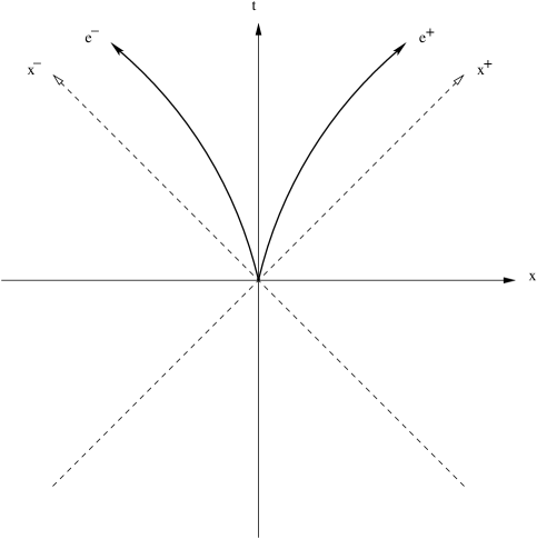
Figure 2: The evolution of an $e^{+}e^{-}$ pair. Note that the electron does not appear beyond a certain value of $x^{+}$.

It remains to compute the probability for pair creation Prob($e^{+}$) at time $x^{+}>X(k^{+})$. From the previous discussion this should be given by the relation,

$$\lim_{L\to\infty}\sqrt{2}\Bigl{\langle}\Omega\Bigl{|}\widetilde{\psi}_{+}^{\dagger}(x^{+},q^{+})\,\widetilde{\psi}_{+}(x^{+},k^{+})\Bigr{|}\Omega\Bigr{\rangle}=\Bigl{[}1-{\rm Prob}(e^{+})\Bigr{]}2\pi\delta(k^{+}-q^{+})\;.$$ (46)

To take the distributional limit rigorously we first smear with test functions $f^{*}(k^{+})$ and $f(q^{+})$,

$$\int_{-\infty}^{+\infty}{{dk^{+}}\over{2\pi}}f^{*}(k^{+})\int_{-\infty}^{+\infty}{{dq^{+}}\over{2\pi}}f(q^{+})\sqrt{2}\Bigl{\langle}\Omega\Bigl{|}\widetilde{\psi}_{+}^{\dagger}(x^{+},q^{+})\,\widetilde{\psi}_{+}(x^{+},k^{+})\Bigr{|}\Omega\Bigr{\rangle}=$$ (47)

$$\sqrt{2}\int_{-\infty}^{+\infty}{{dk^{+}}\over{2\pi}}f^{*}(k^{+})\int_{-\infty}^{+\infty}{{dq^{+}}\over{2\pi}}f(q^{+})\int_{-L}^{\infty}dve^{i(k^{+}+i/L)v}\int_{-L}^{\infty}dze^{-i(q^{+}-i/L)z}$$

$$\times\Biggl{\{}{\cal E}(0,x^{+};k^{+}){\cal E}^{*}(0,x^{+};q^{+})\Bigl{\langle}\Omega\Bigl{|}\psi_{+}^{\dagger}(0,z)\psi_{+}(0,v)\Bigr{|}\Omega\Bigr{\rangle}$$

$$-{im\over 2}\int_{0}^{x^{+}}due^{-ieA_{-}(u)(v+L)}{\cal E}(u,x^{+};k^{+}){\cal E}^{*}\Bigl{\langle}\Omega\Bigl{|}\psi_{+}^{\dagger}(0,z)\gamma^{-}\psi_{-}(u,-L)\Bigr{|}\Omega\Bigr{\rangle}$$

$$+{im\over 2}\int_{0}^{x^{+}}dye^{ieA_{-}(y)(z+L)}{\cal E}{\cal E}^{*}(y,x^{+};q^{+})\Bigl{\langle}\Omega\Bigl{|}\psi_{-}^{\dagger}(y,-L)\gamma^{+}\psi_{+}(0,v)\Bigr{|}\Omega\Bigr{\rangle}$$

$$+{{m^{2}}\over 2}\int_{0}^{x^{+}}due^{-ieA_{-}(u)(v+L)}{\cal E}(u,x^{+};k^{+})\int_{0}^{x^{+}}dye^{ieA_{-}(y)(z+L)}{\cal E}^{*}(y,x^{+};q^{+})$$

$$\hskip 170.71652pt\times\Bigl{\langle}\Omega\Bigl{|}\psi_{-}^{\dagger}(y,-L)\psi_{-}(u,-L)\Bigr{|}\Omega\Bigr{\rangle}\Biggr{\}}\;.$$

As noted in the previous section, the $\pm$ cross correlators vanish in the large $L$ limit. Therefore only the first ($++$) and the fourth ($--$) terms in (47) make a non-vanishing contribution in the $L\to\infty$ limit. The $++$ term gives,

$$\hskip 28.45274pt\int_{-\infty}^{\infty}{{dk^{+}}\over{2\pi}}f^{*}(k^{+})\int_{-\infty}^{\infty}{{dq^{+}}\over{2\pi}}f(q^{+})\int_{-L}^{\infty}dve^{i(k^{+}+i/L)v}\int_{-L}^{\infty}dze^{-i(q^{+}-i/L)z}$$ (52)

$$\hskip 85.35826pt\times\int_{-\infty}^{0}{{dp^{+}}\over{2\pi}}e^{-ip^{+}(v-z)}{\cal E}(0,x^{+};k^{+}){\cal E}^{*}(0,x^{+};q^{+})\;,\qquad$$

$$=\int_{-\infty}^{0}{{dp^{+}}\over{2\pi}}\int_{-\infty}^{+\infty}{{dk^{+}}\over{2\pi}}{{e^{-i[k^{+}-p^{+}+i/L]L}}\over{k^{+}-p^{+}+i/L}}{\cal E}(0,x^{+};k^{+})f^{*}(k^{+})$$

$$\hskip 85.35826pt\times\int_{-\infty}^{+\infty}{{dq^{+}}\over{2\pi}}{{e^{i(q^{+}-p^{+}-i/L)L}}\over{q^{+}-p^{+}-i/L}}{\cal E}^{*}(0,x^{+};q^{+})f(q^{+})\;,\qquad$$

$$=\int_{-\infty}^{0}{{dp^{+}}\over{2\pi}}\int_{-\infty}^{+\infty}{{da}\over{2\pi}}{{e^{-i(a+i)}}\over{a+i}}{\cal E}(0,x^{+};p^{+}+a/L)f^{*}(p^{+}+a/L)$$

$$\hskip 56.9055pt\times\int_{-\infty}^{+\infty}{{db}\over{2\pi}}{{e^{i(b-i)}}\over{b-i}}{\cal E}^{*}(0,x^{+};p^{+}+b/L)f(p^{+}+b/L)\;,$$

$$\longrightarrow\int_{-\infty}^{0}{{dp^{+}}\over{2\pi}}\Bigl{\|}f(p^{+})\Bigr{\|}^{2}\int_{-\infty}^{+\infty}{{da}\over{2\pi}}{{e^{-i(a+i)}}\over{a+i}}\int_{-\infty}^{+\infty}{{db}\over{2\pi}}{{e^{i(b-i)}}\over{b-i}}\;,$$

$$=\int_{-\infty}^{0}{{dp^{+}}\over{2\pi}}\Bigr{\|}f(p^{+})\Bigr{\|}^{2}\;.$$

Before reducing the $--$ term of (47) it is useful to recall the integral [15],

$$\int_{-\infty}^{\infty}{da\over 2\pi}{e^{-i(a+i)}\over a+i}\exp\Bigl{[}-ix\Bigl{(}\ln(a+i)-i\pi\Bigr{)}\Bigr{]}={-ie^{-\pi x/2}\over\Gamma(1+ix)}\;,$$ (53)

and the identity due to Lobachevskiy [26],

$${1\over\Gamma(1+ix)\Gamma(1-ix)}={\sinh(\pi x)\over\pi x}\;,$$ (54)

both valid for real, positive $x$. We must also introduce the function,

$$\lambda(p^{+})\equiv{m^{2}\over 2|e|E(X(p^{+}))}\;.$$ (55)

The large $L$ limit of the $--$ term proceeds in a similar fashion to that of the $++$ term. The steps are,

$${{m^{2}}\over 2}\int{{dk^{+}}\over{2\pi}}f^{*}(k^{+})\int{{dq^{+}}\over{2\pi}}f(q^{+})\int_{-L}^{\infty}dve^{i(k^{+}+i/L)v}\int_{-L}^{\infty}dze^{-i(q^{+}-i/L)z}$$ (61)

$$\times\int_{0}^{x^{+}}due^{-ieA_{-}(u)(v+L)}{\cal E}(u,x^{+};k^{+})\int_{0}^{x^{+}}dye^{ieA_{-}(y)(z+L)}{\cal E}^{*}(y,x^{+};q^{+})$$

$$\times\Biggl{[}{1\over 2}\delta(u-y)+{i\over{2\pi}}{\cal P}\Bigl{(}{1\over{u-y}}\Bigr{)}\Biggr{]}={{m^{2}}\over 2}\int_{0}^{x^{+}}du\int_{0}^{x^{+}}dy{i\over{2\pi}}{\cal P}\Bigl{(}{1\over u-y}\Bigr{)}$$

$$\hskip 28.45274pt\times\int_{-\infty}^{\infty}{{dk^{+}}\over{2\pi}}{e^{-i(k^{+}+i/L)L}\over{k^{+}-eA_{-}(u)+i/L}}{\cal E}(u,x^{+};k^{+})f^{*}(k^{+})$$

$$\hskip 42.67912pt\times\int_{-\infty}^{\infty}{dq^{+}\over 2\pi}{e^{i(q^{+}-i/L)L}\over q^{+}-eA_{-}(y)-i/L}{\cal E}^{*}(y,x^{+};q^{+})f(q^{+})$$

$$+{{m^{2}}\over 4}\int_{0}^{x^{+}}du\int_{-\infty}^{\infty}{{dk^{+}}\over{2\pi}}{e^{-i(k^{+}+i/L)L}\over{k^{+}-eA_{-}(u)+i/L}}{\cal E}(u,x^{+};k^{+})f^{*}(k^{+})$$

$$\hskip 56.9055pt\times\int_{-\infty}^{\infty}{{dq^{+}}\over{2\pi}}{e^{i(q^{+}-i/L)L}\over{q^{+}-eA_{-}(u)-i/L}}{\cal E}^{*}(u,x^{+};q^{+})f(q^{+})\;,$$

$$={{m^{2}}\over 2}\int_{0}^{x^{+}}du\int_{-(eA_{-}(x^{+})-eA_{-}(u))L}^{eA_{-}(u)L}{{dc}\over{2\pi}}{i\over L}{\cal P}\Biggl{(}{X^{\prime}(eA_{-}(u)-c/L)\over u-X(eA_{-}(u)-c/L)}\Biggr{)}$$

$$\times\int_{-\infty}^{\infty}{{da}\over{2\pi}}{e^{-i(a+i)}\over{a+i}}{\cal E}\Bigl{(}u,x^{+};eA_{-}(u)+\frac{a}{L}\Bigr{)}f^{*}\Bigl{(}eA_{-}(u)+\frac{a}{L}\Bigr{)}\int_{-\infty}^{\infty}{{db}\over{2\pi}}{e^{i(b-c-i)}\over{b-i}}$$

$$\hskip 14.22636pt\times{\cal E}^{*}\Biggl{(}X\Bigl{(}eA_{-}(u)-\frac{c}{L}\Bigr{)},x^{+};eA_{-}(u)+\frac{b-c}{L}\Biggr{)}f\Bigl{(}eA_{-}(u)+\frac{b-c}{L}\Bigr{)}$$

$$+{{m^{2}}\over 4}\int_{0}^{x^{+}}du\int_{-\infty}^{\infty}{{da}\over{2\pi}}{e^{-i(a+i)}\over{a+i}}{\cal E}\Bigl{(}u,x^{+};eA_{-}(u)+\frac{a}{L}\Bigr{)}f^{*}\Bigl{(}eA_{-}(u)+\frac{a}{L}\Bigr{)}$$

$$\hskip 28.45274pt\times\int_{-\infty}^{\infty}{{db}\over{2\pi}}{e^{i(b-i)}\over{b-i}}{\cal E}^{*}\Bigl{(}u,x^{+};eA_{-}(u)+\frac{b}{L}\Bigr{)}f\Bigl{(}eA_{-}(u)+\frac{b}{L}\Bigr{)}\;,$$

$$\longrightarrow{{m^{2}}\over 2}\int_{0}^{x^{+}}du\Bigl{\|}f\Bigl{(}eA_{-}(u)\Bigr{)}\Bigr{\|}^{2}\int_{-\infty}^{\infty}{{da}\over{2\pi}}{e^{-i(a+i)}\over{a+i}}e^{-i\lambda\Bigl{(}eA_{-}(u)\Bigr{)}\Bigl{(}\ln(a+i)-i\pi\Bigr{)}}$$

$$\hskip 14.22636pt\times\int_{-\infty}^{\infty}{{db}\over{2\pi}}{e^{i(b-i)}\over{b-i}}e^{i\lambda\Bigl{(}eA_{-}(u)\Bigr{)}\Bigl{(}\ln(b-i)+i\pi\Bigr{)}}\Biggl{\{}\frac{1}{2}+\int_{-\infty}^{\infty}{{dc}\over{2\pi}}{\cal P}\Bigl{(}{ie^{-ic}\over c}\Bigr{)}\Biggr{\}}\;,$$

$$={{m^{2}}\over 2}\int_{0}^{x^{+}}du\Bigl{\|}f\Bigl{(}eA_{-}(u)\Bigr{)}\Bigr{\|}^{2}{{-ie^{-\pi\lambda(eA_{-}(u))/2}}\over{\Gamma(1+i\lambda(eA_{-}(u)))}}\;{{ie^{-\pi\lambda(eA_{-}(u))/2}}\over{\Gamma(1-i\lambda(eA_{-}(u)))}}\;,$$

$$=\int_{0}^{x^{+}}du\Bigl{\|}f\Bigl{(}eA_{-}(u)\Bigr{)}\Bigr{\|}^{2}\Bigl{[}1-e^{-2\pi\lambda(eA_{-}(u))}\Bigr{]}\frac{1}{2\pi}eA^{\prime}_{-}\Bigl{(}X(eA_{-}(u))\Bigr{)}\;,$$

$$=\int_{0}^{eA_{-}(x^{+})}{{dp^{+}}\over{2\pi}}\Bigl{\|}f(p^{+})\Bigr{\|}^{2}\Bigl{[}1-e^{-2\pi\lambda(p^{+})}\Bigr{]}\;.$$

Combining (52) and (61) above we obtain the following relation for the probability of $|\Omega\rangle$ containing a positron of momentum $p^{+}$ at time $x^{+}$,

$$\int_{\infty}^{\infty}{dp^{+}\over 2\pi}\Bigl{\|}f(p^{+})\Bigr{\|}^{2}\Bigl{[}1-{\rm Prob}(e^{+})\Bigr{]}=\int_{\infty}^{0}{dp^{+}\over 2\pi}\Bigl{\|}f(p^{+})\Bigr{\|}^{2}$$ (62)

$$\hskip 113.81102pt+\int_{0}^{eA_{-}(x^{+})}{{dp^{+}}\over{2\pi}}\Bigl{\|}f(p^{+})\Bigr{\|}^{2}\Bigl{[}1-e^{-2\pi\lambda(p^{+})}\Bigr{]}\;.$$

This means that the state remains empty for all $p^{+}<0$ but, for $0<p^{+}<eA_{-}(x^{+})$, it contains a positron with probability,

$${\rm Prob}(e^{+})=e^{-2\pi\lambda(p^{+})}\;.$$ (63)

It should be noted that this result was derived under the assumption that $eA_{-}(x^{+})$ increases monotonically.

5 The vector current

We regulate the various fermion bilinears by gauge invariant point splitting. It suffices to split the two currents $J^{\pm}$ along the directions $x^{\mp}$, respectively,

$$J^{+}(x^{+};x^{-},y^{-}) \equiv {e\over{\sqrt{2}}}e^{ieA_{-}(x^{+})(x^{-}-y^{-})}\Biggl{\{}\psi_{+}^{\dagger}(x^{+},y^{-})\psi_{+}(x^{+},x^{-})$$ (64)

$$\hskip 71.13188pt-{\rm Tr}\Bigl{[}\psi_{+}(x^{+},x^{-})\psi_{+}^{\dagger}(x^{+},y^{-})\Bigr{]}\Biggr{\}}\;,$$

$$J^{-}(x^{+},y^{+};x^{-}) \equiv {e\over{\sqrt{2}}}\Bigl{\{}\psi_{-}^{\dagger}(y^{+},x^{-})\psi_{-}(x^{+},x^{-})$$ (65)

$$\hskip 71.13188pt-{\rm Tr}\Bigl{[}\psi_{-}(x^{+},x^{-})\psi_{-}^{\dagger}(y^{+},x^{-})\Bigr{]}\Biggr{\}}\;.$$

Although these quantities are well regulated and gauge invariant, they are not yet Hermitian. We enforce Hermiticity by taking the symmetric average,

$$J^{+}_{S}(x^{+};x^{-},y^{-}) \equiv {1\over 2}\Bigl{\{}J^{+}(x^{+};x^{-},y^{-})+J^{+}(x^{+};y^{-},x^{-})\Bigr{\}}\;,$$ (66)

$$J^{-}_{S}(x^{+};x^{-},y^{-}) \equiv {1\over 2}\Bigl{\{}J^{-}(x^{+},y^{+};x^{-})+J^{-}(y^{+},x^{+};x^{-})\Bigr{\}}\;.$$ (67)

This could have been done in a single step but it is somewhat more efficient, calculationally, to first compute the expectation values of $J^{\pm}$ in the large $L$ limit and then take the Hermitian average as we also remove the splitting.

Let us begin with $J^{+}$. As explained at the end of Section 3, the first step consists of using our general solution (21) to express the expectation value of $J^{+}(x^{+};x^{-}+\Delta,x^{-})$ as a sum of correlation functions of the initial value operators,

$$\Bigl{\langle}\Omega\Bigl{|}J^{+}(x^{+};x^{-}+\Delta,x^{-})\Bigr{|}\Omega\Bigr{\rangle}={e\over\sqrt{2}}e^{ieA_{-}(x^{+})\Delta}\int_{-\infty}^{\infty}{{dk^{+}}\over{2\pi}}e^{-i(k^{+}+i/L)(x^{-}+\Delta)}$$ (68)

$$\times\int_{-L}^{\infty}dve^{i(k^{+}+i/L)v}\int_{-\infty}^{\infty}{{dq^{+}}\over{2\pi}}e^{i(q^{+}-i/L)x^{-}}\int_{-L}^{\infty}dwe^{-i(q^{+}-i/L)w}\Biggl{\{}{\cal E}(0,x^{+};k^{+})$$

$$\quad\times{\cal E}^{*}(0,x^{+};q^{+})\Bigl{\langle}\Omega\Bigl{|}\psi_{+}^{\dagger}(0,w)\psi_{+}(0,v)-{\rm Tr}\Bigl{[}\psi_{+}(0,v)\psi_{+}^{\dagger}(0,w)\Bigr{]}\Bigr{|}\Omega\Bigr{\rangle}$$

$$+{{im}\over 2}{\cal E}(0,x^{+};k^{+})\int_{0}^{x^{+}}dye^{ieA_{-}(y)(w+L)}{\cal E}^{*}(y,x^{+};q^{+})$$

$$\hskip 42.67912pt\times\Bigl{\langle}\Omega\Bigl{|}\psi_{-}^{\dagger}(y,-L)\gamma^{+}\psi_{+}(0,v)-{\rm Tr}\Bigl{[}\psi_{+}(0,v)\psi_{-}^{\dagger}(y,-L)\gamma^{+}\Bigr{]}\Bigr{|}\Omega\Bigr{\rangle}$$

$$-{{im}\over 2}\int_{0}^{x^{+}}due^{-ieA_{-}(u)(v+L)}{\cal E}(u,x^{+};k^{+}){\cal E}^{*}(0,x^{+};q^{+})$$

$$\hskip 42.67912pt\times\Bigl{\langle}\Omega\Bigl{|}\psi_{+}^{\dagger}(0,w)\gamma^{-}\psi_{-}(u,-L)-{\rm Tr}\Bigl{[}\gamma^{-}\psi_{-}(u,-L)\psi_{+}^{\dagger}(0,w)\Bigr{]}\Bigr{|}\Omega\Bigr{\rangle}$$

$$+{{m^{2}}\over 2}\int_{0}^{x^{+}}due^{-ieA_{-}(u)(v+L)}{\cal E}(u,x^{+};k^{+})\int_{0}^{x^{+}}dye^{ieA_{-}(y)(w+L)}{\cal E}^{*}(y,x^{+};q^{+})$$

$$\hskip 28.45274pt\times\Bigl{\langle}\Omega\Bigl{|}\psi_{-}^{\dagger}(y,-L)\psi_{-}(u,-L)-{\rm Tr}\Bigl{[}\psi_{-}(u,-L)\psi_{-}^{\dagger}(y,-L)\Bigr{]}\Bigr{|}\Omega\Bigr{\rangle}\Biggr{\}}.\quad$$

The various correlation functions which appear in (68) can be read off from relations (37) and (38). First note that the spinor identity,

$$\raise 0.6458pt\hbox{$/$}\kern-5.70007pt{p}\gamma^{0}\pm m\gamma^{0}=\sqrt{2}{\cal P}_{+}p^{+}+\sqrt{2}{\cal P}_{-}p^{-}\pm{m\over\sqrt{2}}(\gamma^{+}+\gamma^{-})\;,$$ (69)

implies the following projections,

$${\cal P}_{+}(\raise 0.6458pt\hbox{$/$}\kern-5.70007pt{p}\gamma^{0}\pm m\gamma^{0}){\cal P}_{+}=\sqrt{2}p^{+}{\cal P}_{+}\;\;,\;\;{\cal P}_{+}(\raise 0.6458pt\hbox{$/$}\kern-5.70007pt{p}\gamma^{0}\pm m\gamma^{0}){\cal P}_{-}\gamma^{+}=\pm\sqrt{2}m{\cal P}_{+}\;,$$ (70)

$$\gamma^{-}{\cal P}_{-}(\raise 0.6458pt\hbox{$/$}\kern-5.70007pt{p}\gamma^{0}\pm m\gamma^{0}){\cal P}_{+}=\pm\sqrt{2}m{\cal P}_{+}\;\;,\;\;{\cal P}_{-}(\raise 0.6458pt\hbox{$/$}\kern-5.70007pt{p}\gamma^{0}\pm m\gamma^{0}){\cal P}_{-}=\sqrt{2}p^{-}{\cal P}_{-}\;.$$ (71)

As with the particle production probability, we can drop the $+-$ and $-+$ correlators in the large $L$ limit. The $++$ and $--$ correlators are,

$$\Bigl{\langle}\Omega\Bigl{|}\psi_{+}^{\dagger}(0,w)\psi_{+}(0,v)-{\rm Tr}\Bigl{[}\psi_{+}(0,v)\psi_{+}^{\dagger}(0,w)\Bigr{]}\Bigr{|}\Omega\Bigr{\rangle}$$ (72)

$$\hskip 56.9055pt=\frac{1}{\sqrt{2}}\Biggl{\{}\int_{-\infty}^{0}{dp^{+}\over 2\pi}-\int_{0}^{\infty}{dp^{+}\over 2\pi}\Biggr{\}}e^{-ip^{+}(v-w)}\;,\;$$

$$\Bigl{\langle}\Omega\Bigl{|}\psi_{-}^{\dagger}(y,-L)\psi_{-}(u,-L)-{\rm Tr}\Bigl{[}\psi_{-}(u,-L)\psi_{-}^{\dagger}(y,-L)\Bigr{]}\Bigr{|}\Omega\Bigr{\rangle}={i\over{\sqrt{2}\pi}}{\cal P}\Bigl{(}{1\over{u-y}}\Bigr{)}\;.$$ (73)

The reduction strategy is quite similar to that used in Section 4 for the probability of particle production. First perform the integrals over $v$ and $w$,

$$\int_{-L}^{\infty}dve^{i(k^{+}+i/L)v}e^{-il^{+}(v+L)}={{ie^{-i(k^{+}+i/L)L}}\over{k^{+}-l^{+}+i/L}}\;.$$ (74)

Next make the appropriate change of change variables from $k^{+}$ and $q^{+}$ to,

$$a\equiv(k^{+}-l^{+})L\;\;\;{\rm and}\;\;\;b\equiv(q^{+}-l^{+})L\;\;,$$ (75)

and take the $L\rightarrow\infty$ limit of the mode functions ${\cal E}$ using,

$$\lim_{L\rightarrow\infty}{\cal E}\Bigl{(}0,x^{+};p^{+}+\frac{a}{L}\Bigr{)}\;{\cal E}^{*}\Bigl{(}0,x^{+};p^{+}+\frac{b}{L}\Bigr{)}$$ (76)

$$\hskip 85.35826pt=\exp\Bigl{[}-2\pi\lambda(p^{+})\theta(p^{+})\theta\Bigl{(}eA_{-}(x^{+})-p^{+}\Bigr{)}\Bigr{]},\;$$

$$\lim_{L\rightarrow\infty}{\cal E}\Bigl{(}X(r^{+}),x^{+};r^{+}+\frac{a}{L}\Bigr{)}\;{\cal E}^{*}\Bigl{(}X\Bigl{(}r^{+}-\frac{c}{L}\Bigr{)},x^{+};r^{+}+\frac{b-c}{L}\Bigr{)}$$ (77)

$$\hskip 85.35826pt=\exp\Bigl{[}\lambda(r^{+})\Bigl{(}-2\pi-i\ln(a+i)+i\ln(b-i)\Bigr{)}\Bigr{]}\;.$$

(We have assumed $r^{+}>0$ in taking the last limit.) Finally the $a$ and $b$ integrations are performed using (53), and the result is simplified with the identity (54) of Lobachevskiy.

Applying this procedure to the $++$ term gives,

$$J^{+}_{(++)}={e\over 2}e^{ieA_{-}(x^{+})\Delta}\Biggl{\{}\int_{-\infty}^{0}{{dp^{+}}\over{2\pi}}-\int_{0}^{\infty}{{dp^{+}}\over{2\pi}}\Biggr{\}}\int_{-\infty}^{\infty}{{dk^{+}}\over{2\pi}}{{e^{-i(k^{+}+i/L)(L+x^{-}+\Delta)}}\over{k^{+}-p^{+}+i/L}}$$ (82)

$$\hskip 71.13188pt\times{\cal E}(0,x^{+};k^{+})\int_{-\infty}^{\infty}{{dq^{+}}\over{2\pi}}{{e^{i(q^{+}-i/L)(L+x^{-})}}\over{q^{+}-p^{+}-i/L}}{\cal E}^{*}(0,x^{+};q^{+})\;,$$

$$={e\over 2}\Biggl{\{}\int_{-\infty}^{0}{{dp^{+}}\over{2\pi}}-\int_{0}^{\infty}{{dp^{+}}\over{2\pi}}\Biggr{\}}e^{-i(p^{+}-eA_{-}(x^{+}))\Delta}\int_{-\infty}^{\infty}{{da}\over{2\pi}}{{e^{-i(a+i)(1+(x^{-}+\Delta)/L)}}\over{a+i}}$$

$$\hskip 42.67912pt\times{\cal E}\Bigl{(}0,x^{+};p^{+}+\frac{a}{L}\Bigr{)}\int_{-\infty}^{\infty}{{db}\over{2\pi}}{{e^{i(b-i)(1+x^{-}/L)}}\over{b-i}}{\cal E}^{*}\Bigl{(}0,x^{+};p^{+}+\frac{b}{L}\Bigr{)},\quad$$

$$\longrightarrow{e\over 2}\Biggl{\{}\int_{-\infty}^{0}-\int_{eA_{-}(x^{+})}^{\infty}-\int_{0}^{eA_{-}(x^{+})}e^{-2\pi\lambda(p^{+})}\Biggr{\}}{dp^{+}\over 2\pi}e^{-i[p^{+}-eA_{-}(x^{+})]\Delta}\;,$$

$$={e\over 2}\Biggl{\{}\int_{-\infty}^{eA_{-}(x^{+})}-\int_{eA_{-}(x^{+})}^{\infty}-\int_{0}^{eA_{-}}\Bigl{[}1+e^{-2\pi\lambda(p^{+})}\Bigr{]}\Biggr{\}}{{dp^{+}}\over{2\pi}}e^{-i[p^{+}-eA_{-}]\Delta}\;,$$

$$={e\over 2}\Biggl{\{}{i\over{\pi\Delta}}-\int_{0}^{eA_{-}(x^{+})}{{dp^{+}}\over{2\pi}}\Bigl{[}1+e^{-2\pi\lambda(p^{+})}\Bigr{]}e^{-i[p^{+}-eA_{-}(x^{+})]\Delta}\Biggr{\}}\;.$$

We begin the reduction of the $--$ term by changing variables from $u$ and $y$ to $r^{+}\equiv eA_{-}(u)$ and $s^{+}\equiv eA_{-}(y)$,

$$J^{+}_{(--)}={e\over{m^{2}}}e^{ieA_{-}(x^{+})\Delta}\int_{0}^{eA_{-}(x^{+})}dr^{+}\lambda(r^{+})\int_{0}^{eA_{-}(x^{+})}ds^{+}\lambda(s^{+})$$ (84)

$$\times{i\over\pi}{\cal P}\Biggl{(}{1\over X(r^{+})-X(s^{+})}\Biggr{)}\int_{-\infty}^{\infty}{{dk^{+}}\over{2\pi}}{{e^{-i(k^{+}+i/L)(L+x^{-}+\Delta)}}\over{k^{+}-r^{+}+i/L}}{\cal E}\Bigl{(}X(r^{+}),x^{+};k^{+}\Bigr{)}$$

$$\hskip 85.35826pt\times\int_{-\infty}^{\infty}{{dq^{+}}\over{2\pi}}{{e^{i(q^{+}-i/L)(L+x^{-})}}\over{q^{+}-s^{+}-i/L}}{\cal E}^{*}\Bigl{(}X(s^{+}),x^{+};q^{+}\Bigr{)}\;,$$

$$={ie\over\pi m^{2}}\int_{0}^{eA_{-}(x^{+})}dr^{+}\lambda(r^{+})e^{-i[r^{+}-eA_{-}(x^{+})]\Delta}\int_{0}^{eA_{-}(x^{+})}ds^{+}\lambda(s^{+})$$

$$\times{\cal P}\Biggl{(}{e^{-i(r^{+}-s^{+})(L+x^{-})}\over X(r^{+})-X(s^{+})}\Biggr{)}\int_{-\infty}^{\infty}{{da}\over{2\pi}}{{e^{-i(a+i)[1+(x^{-}+\Delta)/L]}}\over{a+i}}{\cal E}\Bigl{(}X(r^{+}),x^{+};r^{+}+\frac{a}{L}\Bigr{)}$$

$$\hskip 85.35826pt\times\int_{-\infty}^{\infty}{{db}\over{2\pi}}{{e^{i(b-i)(1+x^{-}/L)}}\over{b-i}}{\cal E}^{*}\Bigl{(}X(s^{+}),x^{+};s^{+}+\frac{b}{L}\Bigr{)}\;.$$

Now change variables from $s^{+}$ to $c\equiv(r^{+}-s^{+})L$ and expand,

$$X(s^{+})=X(r^{+}-c/L)=X(r^{+})-{{2\lambda(r^{+})}\over{m^{2}}}{c\over L}+{\cal O}(L^{-2})\;.$$ (85)

The large $L$ limit is therefore,

$$J^{+}_{(--)}\longrightarrow{e\over 2}\int_{0}^{eA_{-}(x^{+})}dr^{+}\lambda(r^{+})e^{-i[r^{+}-eA_{-}(x^{+})]\Delta}e^{-2\pi\lambda(r^{+})}\int_{-\infty}^{\infty}{dc\over\pi}{{\sin{c}}\over c}$$ (89)

$$\hskip 28.45274pt\times\int_{-\infty}^{\infty}{{da}\over{2\pi}}{{e^{-i(a+i)}}\over{a+i}}e^{-i\lambda(r^{+})\ln(a+i)}\int_{-\infty}^{\infty}{{db}\over{2\pi}}{{e^{i(b-i)}}\over{b-i}}e^{i\lambda(r^{+})\ln(b-i)},$$

$$={e\over 2}\int_{0}^{eA_{-}(x^{+})}dr^{+}\lambda(r^{+})e^{-i[r^{+}-eA_{-}(x^{+})]\Delta}{e^{-\pi\lambda(r^{+})}\over\|\Gamma(1+i\lambda(r^{+}))\|^{2}}\;,$$

$$={e\over 2}\int_{0}^{eA_{-}(x^{+})}dr^{+}\lambda(r^{+})e^{-i[(r^{+}-eA_{-}(x^{+})]\Delta}\Biggl{[}{1-e^{-2\pi\lambda(r^{+})}\over 2\pi\lambda(r^{+})}\Biggr{]}\;,$$

$$={e\over 2}\int_{0}^{eA_{-}(x^{+})}{{dr^{+}}\over{2\pi}}e^{-i[(r^{+}-eA_{-}(x^{+})]\Delta}\Bigl{[}1-e^{-2\pi\lambda(r^{+})}\Bigr{]}\;.$$

Adding the $++$ and $--$ contributions gives,

$$\lim_{L\rightarrow\infty}\Bigl{\langle}\Omega\Bigl{|}J^{+}(x^{+};x^{-}+\Delta,x^{-})\Bigr{|}\Omega\Bigr{\rangle}={e\over 2}\Biggl{\{}{i\over{\pi\Delta}}$$ (90)

$$\hskip 85.35826pt-2\int_{0}^{eA_{-}(x^{+})}{{dp^{+}}\over{2\pi}}e^{-2\pi\lambda(p^{+})}e^{-i[p^{+}-eA_{-}(x^{+})]\Delta}\Biggr{\}}.$$

The linear divergence vanishes upon Hermitization, so we can take the splitting parameter $\Delta$ to zero,

$$\lim_{L\rightarrow\infty}\Bigl{\langle}\Omega\Bigl{|}J^{+}_{S}(x^{+};x^{-}+\Delta,x^{-})\Bigr{|}\Omega\Bigr{\rangle}$$ (91)

$$= -e\int_{0}^{eA_{-}(x^{+})}{{dp^{+}}\over{2\pi}}e^{-2\pi\lambda(p^{+})}\cos\Bigl{[}\Bigl{(}p^{+}-eA_{-}(x^{+})\Bigr{)}\Delta\Bigr{]}\;,$$

$$\longrightarrow -e\int_{0}^{eA_{-}(x^{+})}{{dp^{+}}\over{2\pi}}e^{-2\pi\lambda(p^{+})}\;.$$ (92)

The interpretation of this result is straightforward. $J^{+}$ is the light-cone charge density, so we expect it to grow as more and more positrons are created. (Recall that the electrons immediately leave the light-cone manifold as depicted in Fig. 2.) Each positron carries charge $-e$; the probability for mode $p^{+}$ to be created is $\exp[-2\pi\lambda(p^{+})]$ (from equation (63)); and the number of modes per unit volume is $dp^{+}/{2\pi}$. We therefore expect the increment to obey,

$$dJ^{+}=\Bigl{(}-e\Bigr{)}\times\Bigl{(}e^{-2\pi\lambda(p^{+})}\Bigr{)}\times\Bigl{(}{dp^{+}\over 2\pi}\Bigr{)}\;.$$ (93)

For monotonically increasing $eA_{-}(x^{+})$, all the modes in the interval $0<p^{+}<eA_{-}(x^{+})$ will have contributed, which gives precisely (92). This is a powerful check on the fundamental correctness of our formalism as well as on our proper application of it.

It remains to compute the expectation value of $J^{-}$. First note that we can express $J^{-}(x^{+},y^{+};x^{-})$ in terms of $\psi_{+}$ using the field equation $\psi_{-}=(i/m)\gamma^{+}i\partial_{+}\psi_{+}$,

$$J^{-}(x^{+},y^{+};x^{-})={\sqrt{2}e\over m^{2}}{\partial\over\partial x^{+}}{\partial\over{\partial y^{+}}}\Biggl{\{}\psi_{+}^{\dagger}(y^{+},x^{-})\psi_{+}(x^{+},x^{-})$$ (94)

$$\hskip 170.71652pt-{\rm Tr}\Bigl{[}\psi_{+}(x^{+},x^{-})\psi_{+}^{\dagger}(y^{+},x^{-})\Bigr{]}\Biggr{\}}.\quad$$

As before we can use the general solution (21) to reduce the expectation value of this operator to a sum of four correlators on the initial value surface. Also as before, the $+-$ and $-+$ correlators vanish for infinite $L$. We therefore require only,

$$J^{-}_{(++)}\equiv{e\over{m^{2}}}{\partial\over{\partial x^{+}}}{\partial\over{\partial y^{+}}}\int_{-\infty}^{\infty}{dk^{+}\over 2\pi}e^{-i(k^{+}+i/L)(x^{-}+L)}{\cal E}(0,x^{+};k^{+})$$ (95)

$$\times\int_{-\infty}^{\infty}{{dq^{+}}\over{2\pi}}e^{i(q^{+}-i/L)(x^{-}+L)}{\cal E}^{*}(0,y^{+};q^{+})$$

$$\hskip 28.45274pt\times\Biggl{\{}\int_{-\infty}^{0}{dp^{+}\over 2\pi}-\int_{0}^{\infty}{dp^{+}\over 2\pi}\Biggr{\}}{1\over{(k^{+}-p^{+}+i/L)(q^{+}-p^{+}-i/L)}},\quad$$

and,

$$J^{-}_{(--)}\equiv{ie\over 2\pi}{\partial\over{\partial x^{+}}}{\partial\over{\partial y^{+}}}\int_{-\infty}^{\infty}{{dk^{+}}\over{2\pi}}e^{-i(k^{+}+i/L)(x^{-}+L)}\int_{-\infty}^{\infty}{{dq^{+}}\over{2\pi}}e^{i(q^{+}-i/L)(x^{-}+L)}$$ (96)

$$\times\int_{0}^{x^{+}}{du\;{\cal E}(u,x^{+};k^{+})\over{k^{+}-eA_{-}(u)+i/L}}\int_{0}^{y^{+}}{dz\;{\cal E}^{*}(z,y^{+};q^{+})\over{q^{+}-eA_{-}(z)-i/L}}{\cal P}\Biggl{(}{1\over{u-z}}\Biggr{)}\;.$$

After taking the $x^{+}$ and $y^{+}$ derivatives, and performing the $p^{+}$ integrals, the $++$ term becomes,

$$J^{-}_{(++)}=-{{iem^{2}}\over 4\pi}\int_{-\infty}^{\infty}{{dk^{+}}\over{2\pi}}{{e^{-i(k^{+}+i/L)(x^{-}+L)}}\over{k^{+}-eA_{-}(x^{+})+i/L}}{\cal E}(0,x^{+};k^{+})\int_{-\infty}^{\infty}{dq^{+}\over 2\pi}$$ (97)

$$\times{e^{i(q^{+}-i/L)(x^{-}+L)}\over q^{+}-eA_{-}(y^{+})-i/L}{{\cal E}^{*}(0,y^{+};q^{+})\over{k^{+}-q^{+}+2i/L}}\Biggl{[}\pi+i\ln\Biggl{(}{{k^{+}+i/L}\over{q^{+}-i/L}}\Biggr{)}\Biggr{]}\;.$$

Acting the $x^{+}$ derivative on $J^{-}_{(--)}$ produces two terms, one where the derivative hits the upper limit of the $u$ integration and the other where it hits the mode function ${\cal E}(u,x^{+};k^{+})$. The first of these terms simply sets $u=x^{+}$, which makes the mode function unity. The second term brings down a factor of $-m^{2}/2$ divided by $[k^{+}-eA_{-}(x^{+})+i/L]$. Acting the $y^{+}$ derivative gives two similar terms, with the result that $J^{-}_{(--)}$ can be written as the sum of the following four expressions,

$$J^{-}_{(a)}={{ie}\over{2\pi}}{{e^{-ie[A_{-}(x^{+})-A_{-}(y^{+})](x^{-}+L)}}\over{x^{+}-y^{+}}}\;,$$ (98)

$$J^{-}_{(b)}={iem^{2}\over 4\pi}\int_{0}^{y^{+}}{\cal P}\Bigl{(}{dz\over x^{+}-z}\Bigr{)}$$ (99)

$$\hskip 28.45274pt\times\int_{-\infty}^{\infty}{{dq^{+}}\over{2\pi}}{{e^{i[q^{+}-eA_{-}(x^{+})-i/L](x^{-}+L)}{\cal E}^{*}(z,y^{+};q^{+})}\over{[q^{+}-eA_{-}(z)-i/L][q^{+}-eA_{-}(y^{+})-i/L]}}\;,$$

$$J^{-}_{(c)}={iem^{2}\over 4\pi}\int_{0}^{x^{+}}{\cal P}\Bigl{(}{du\over{u-y^{+}}}\Bigr{)}$$ (100)

$$\hskip 28.45274pt\times\int_{-\infty}^{\infty}{{dk^{+}}\over{2\pi}}{{e^{-i[k^{+}-eA_{-}(y^{+})+i/L](x^{-}+L)}{\cal E}(u,x^{+};k^{+})}\over{[k^{+}-eA_{-}(u)+i/L][k^{+}-eA_{-}(x^{+})+i/L]}}\;,$$

$$J^{-}_{(d)}={{iem^{4}}\over 8\pi}\int_{0}^{x^{+}}du\int_{0}^{y^{+}}dz{\cal P}\Bigl{(}{1\over{u-z}}\Bigr{)}$$ (101)

$$\hskip 14.22636pt\times\int_{-\infty}^{\infty}{{dk^{+}}\over{2\pi}}{{e^{-i(k^{+}+i/L)(x^{-}+L)}{\cal E}(u,x^{+};k^{+})}\over{[k^{+}-eA_{-}(u)+i/L][k^{+}-eA_{-}(x^{+})+i/L]}}$$

$$\hskip 28.45274pt\times\int_{-\infty}^{\infty}{{dq^{+}}\over{2\pi}}{{e^{i(q^{+}-i/L)(x^{-}+L)}{\cal E}^{*}(z,y^{+};q^{+})}\over{[q^{+}-eA_{-}(z)-i/L][q^{+}-eA_{-}(y^{+})-i/L]}}\;.$$

At this point the reduction of $\langle J^{-}\rangle$ deviates somewhat from the procedure we used for $\langle J^{+}\rangle$, and it is well to comment on the reasons for this before proceeding. First note that the only ultraviolet divergent contribution comes from the single term — $J^{-}{(a)}$ — for which we can obtain an explicit result in terms of elementary functions before taking the large $L$ limit. All the other terms remain finite as we take $y^{+}\longrightarrow x^{+}$ at fixed $L$. Second, note that all the other terms vanish at $x^{-}=-L$ because we can close the $k^{+}$ and $q^{+}$ contours above and below, respectively, where the integrand in analytic. The physical reason for this is that $x^{-}=-L$ is the initial value surface upon which our state $|\Omega\rangle$ agrees with the $A_{-}=0$ vacuum that has zero current.

A third important observation is that all the other terms diverge linearly when the large $L$ limit is taken at finite $x^{-}$ after setting $y^{+}=x^{+}$. The physical reason for this is that, just as $J^{+}$ is the light-cone charge density, so $J^{-}$ gives the light-cone charge flux. Although the electrons make no contribution to $J^{+}$ because they immediately leave the manifold moving parallel to the $x^{-}$ axis, they do contribute to $J^{-}$ for the very same reason. The electron current flowing through any fixed value of $x^{-}$ consists of the flux originating in each element $dx^{-}$, all the way back to $x^{-}=-L$. In analogy with (93) we expect the increment from each volume element $dx^{-}$ to be the electron charge times the probability for creation times the rate at which modes pass through the critical point $p^{+}=eA_{-}(x^{+})$,

$$dJ^{-}=\Bigl{(}+e\Bigr{)}\times\Bigl{(}e^{-2\pi\lambda(eA_{-}(x^{+}))}\Bigr{)}\times\Bigl{(}{eA_{-}^{\prime}(x^{+})dx^{-}\over 2\pi}\Bigr{)}\;.$$ (102)

Since this expression does not depend upon $x^{-}$, integrating it from $-L$ to $x^{-}$ adds a factor of $(L+x^{-})$, which is the origin of the linear divergence in the large $L$ limit.

This last observation implies that we cannot take the large $L$ limit in evaluating the expectation value of $J^{-}$. However, the fact that we know the value of $J^{-}$ at $x^{-}=-L$ (zero) suggests that we can equally well compute the expectation value of $\partial_{-}J^{-}$ — which does have a finite large $L$ limit — and then integrate to obtain the undifferentiated current. That is the strategy we shall follow. To simplify the computation we shall also take the coincidence limit before letting $L$ go to infinity.

From (97) we obtain,

$$\partial_{-}J^{-}_{(++)}={iem^{2}\over 4\pi}\int_{-\infty}^{\infty}{{dk^{+}}\over{2\pi}}{{e^{-i(k^{+}+i/L)(x^{-}+L)}}\over{k^{+}-eA_{-}(x^{+})+i/L}}{\cal E}(0,x^{+};k^{+})$$ (103)

$$\times\int_{-\infty}^{\infty}{dq^{+}\over 2\pi}{e^{i(q^{+}-i/L)(x^{-}+L)}{\cal E}^{*}(0,y^{+};q^{+})\over{q^{+}-eA_{-}(y^{+})-i/L}}\Biggl{[}i\pi-\ln\Biggl{(}{k^{+}+i/L\over{q^{+}-i/L}}\Biggr{)}\Biggr{]}.\quad$$

Making the change of variables $a\equiv[k^{+}-eA_{-}(x^{+})]L$ and $b\equiv[q^{+}-eA_{-}(y^{+})]L$, and taking the limits $x^{+}\to y^{+}$ and $L\to\infty$ gives,

$$\partial_{-}J^{-}_{(++)}\longrightarrow-{{em^{2}}\over 4}\int_{-\infty}^{\infty}{{da}\over{2\pi}}{{e^{-i(a+i)}}\over{a+i}}e^{i\lambda(eA_{-}(x^{+}))\ln(a+i)}$$ (105)

$$\hskip 85.35826pt\times\int_{-\infty}^{\infty}{{db}\over{2\pi}}{{e^{i(b-i)}}\over{b-i}}e^{-i\lambda(eA_{-}(x^{+}))\ln(b-i)}\;,$$

$$=-{{e^{2}A^{\prime}_{-}(x^{+})}\over{4\pi}}\Bigl{[}1-e^{-2\pi\lambda(eA_{-}(x^{+}))}\Bigr{]}\;.$$

To evaluate the $--$ terms we first note that the coincidence limit of $\partial_{-}J^{-}_{(a)}$ is real and finite,

$$\partial_{-}J^{-}_{(4a)}\to{{e^{2}A^{\prime}_{-}(x^{+})}\over{2\pi}}\;.$$ (106)

Next combine the coincidence limits of the $b$, $c$ and $d$ terms to reach,

$$\lim_{y^{+}\rightarrow x^{+}}\partial_{-}J^{-}_{(b-d)}=-{{iem^{2}}\over 4\pi}{\partial\over{\partial x^{+}}}\int_{0}^{x^{+}}du\int_{0}^{x^{+}}{\cal P}\Bigl{(}{dz\over{u-z}}\Bigr{)}\int_{-\infty}^{\infty}{dk^{+}\over 2\pi}{\cal E}(u,x^{+};k^{+})$$ (107)

$$\hskip 14.22636pt\times{e^{-i(k^{+}+i/L)(x^{-}+L)}\over{k^{+}-eA_{-}(u)+i/L}}\int_{-\infty}^{\infty}{dq^{+}\over 2\pi}{e^{i(q^{+}-i/L)(x^{-}+L)}{\cal E}^{*}(z,x^{+};q^{+})\over{q^{+}-eA_{-}(z)-i/L}}.\qquad$$

Now change variables from $k^{+}$, $q^{+}$ and $z$ to,

$$a\equiv[k^{+}-eA_{-}(u)]L\quad,\quad b\equiv[q^{+}-eA_{-}(z)]L\quad,\quad c\equiv e[A_{-}(u)-A_{-}(z)]L\;,$$ (108)

and take the large $L$ limit,

$$\lim_{L\rightarrow\infty}\lim_{y^{+}\rightarrow x^{+}}\partial_{-}J^{-}_{(b-d)}=-{{em^{2}}\over 4}{\partial\over{\partial x^{+}}}\int_{0}^{x^{+}}due^{-2\pi\lambda(eA_{-}(u))}\int_{-\infty}^{\infty}dc{\sin c\over c}$$ (110)

$$\times\int_{-\infty}^{\infty}{{da}\over{2\pi}}{{e^{-i(a+i)}}\over{a+i}}e^{-i\lambda(eA_{-}(u))\ln(a+i)}\int_{-\infty}^{\infty}{{db}\over{2\pi}}{{e^{i(b-i)}}\over{b-i}}e^{i\lambda(eA_{-}(u))\ln(b-i)},\quad$$

$$=-{{e^{2}A^{\prime}_{-}(x^{+})}\over{4\pi}}\Bigl{[}1-e^{-2\pi\lambda(eA_{-}(x^{+}))}\Bigr{]}\;.$$

Combining with (105) and (106) we obtain,

$$\lim_{L\rightarrow\infty}\lim_{y^{+}\rightarrow x^{+}}\partial_{-}\Bigl{\langle}\Omega\Bigl{|}J^{-}(x^{+},y^{+};x^{-})\Bigr{|}\Omega\Bigr{\rangle}={{e^{2}A^{\prime}_{-}(x^{+})}\over{2\pi}}e^{-2\pi\lambda(eA_{-}(x^{+}))}\;.$$ (111)

Since this is already real, Hermitization makes no change. The fact that these explicit calculations are in complete agreement with our physics-based expectation (102) is another impressive check.

Our final results for the vector current are,

$$\lim_{y^{-}\rightarrow x^{-}}\Bigl{\langle}\Omega\Bigl{|}J^{+}_{S}(x^{+};x^{-},y^{-})\Bigr{|}\Omega\Bigr{\rangle} = -e\int_{0}^{eA_{-}(x^{+})}{dp^{+}\over 2\pi}e^{-2\pi\lambda(p^{+})}+\dots\;,$$ (112)

$$\lim_{y^{-}\rightarrow x^{-}}\Bigl{\langle}\Omega\Bigl{|}J^{-}_{S}(x^{+},y^{+};x^{-})\Bigr{|}\Omega\Bigr{\rangle} = {{e^{2}A^{\prime}_{-}}\over{2\pi}}e^{-2\pi\lambda(eA_{-})}\Bigl{(}L+x^{-}\Bigr{)}+\dots$$ (113)

Here the dots indicate terms which vanish as $L$ goes to infinity. Note that the divergence of the vector current vanishes, as it should.

6 The axial vector anomaly

It is convenient to point split the pseudoscalar in both directions,

$$J_{5}(x^{+},y^{+};x^{-},y^{-})\equiv{1\over\sqrt{8}}\exp\Biggl{[}ie(x^{-}-y^{-})\int_{0}^{1}d\tau A_{-}\Bigl{(}y^{+}+\tau(x^{+}-y^{+})\Bigr{)}\Biggr{]}$$ (114)

$$\times\Biggl{\{}\psi_{-}^{\dagger}(y^{+},y^{-})\gamma^{+}\psi_{+}(x^{+},x^{-})-\psi_{+}^{\dagger}(y^{+},y^{-})\gamma^{-}\psi_{-}(x^{+},x^{-})$$

$$-{\rm Tr}\Bigl{[}\psi_{+}(x^{+},x^{-})\psi_{-}^{\dagger}(y^{+},y^{-})\gamma^{+}\Bigr{]}+{\rm Tr}\Bigl{[}\psi_{-}(x^{+},x^{-})\psi_{+}^{\dagger}(y^{+},y^{-})\gamma^{-}\Bigr{]}\Biggr{\}}.\quad\qquad$$

This can be rewritten in terms of $\psi_{+}$ alone by using (10),

$$J_{5}(x^{+},y^{+};x^{-},y^{-})={-i\over\sqrt{2}m}\exp\Biggl{[}ie(x^{-}-y^{-})\int_{0}^{1}d\tau A_{-}\Bigl{(}y^{+}+\tau(x^{+}-y^{+})\Bigr{)}\Biggr{]}$$ (116)

$$\quad\times\Biggl{(}{\partial\over{\partial x^{+}}}+{\partial\over{\partial y^{+}}}\Biggr{)}\Biggl{\{}\psi_{+}^{\dagger}(y^{+},y^{-})\psi_{+}(x^{+},x^{-})$$

$$\hskip 85.35826pt-{\rm Tr}\Bigl{[}(\psi_{+}(x^{+},x^{-})\psi_{+}^{\dagger}(y^{+},y^{-})\Bigr{]}\Biggr{\}}\qquad\;,$$

$$={-i\over\sqrt{2}m}\Biggl{(}{\partial\over{\partial x^{+}}}+{\partial\over{\partial y^{+}}}-ie{{A_{-}(x^{+})-A_{-}(y^{+})}\over{x^{+}-y^{+}}}(x^{-}-y^{-})\Biggr{)}$$

$$\hskip 14.22636pt\times\exp\Biggl{[}ie(x^{-}-y^{-})\int_{0}^{1}d\tau A_{-}\Bigl{(}y^{+}+\tau(x^{+}-y^{+})\Bigr{)}\Biggr{]}$$

$$\hskip 28.45274pt\times\Biggl{\{}\psi_{+}^{\dagger}(y^{+},y^{-})\psi_{+}(x^{+},x^{-})-{\rm Tr}\Bigl{[}\psi_{+}(x^{+},x^{-})\psi_{+}^{\dagger}(y^{+},y^{-})\Bigr{]}\Biggr{\}}\;.\quad$$

Now take the $+$ coordinates to coincidence,

$$J_{5}(x^{+},x^{+};x^{-},y^{-})={-i\over em}{\partial\over{\partial x^{+}}}J^{+}(x^{+};x^{-},y^{-})$$ (117)

$$\hskip 56.9055pt-{1\over m}A^{\prime}_{-}(x^{+})(x^{-}-y^{-})J^{+}(x^{+};x^{-},y^{-})\;.$$

This strong operator equation is still well regulated by the point splitting of the $-$ coordinates.

In the large $L$ limit the expectation value of (117) gives,

$$\lim_{L\rightarrow\infty}\Bigl{\langle}\Omega\Bigl{|}J_{5}(x^{+},x^{+};x^{-},y^{-})\Bigr{|}\Omega\Bigr{\rangle}$$ (118)

$$={-i\over em}\Biggl{(}{\partial\over{\partial x^{+}}}-ieA^{\prime}_{-}(x^{+})(x^{-}-y^{-})\Biggr{)}\lim_{L\rightarrow\infty}\Bigl{\langle}\Omega\Bigl{|}J^{+}(x^{+};x^{-},y^{-})\Bigr{|}\Omega\Bigr{\rangle}.\quad$$

We computed the expectation value on the right hand side in (90). Substituting this relation and taking the $-$ points to coincidence gives,

$$\lim_{y^{-}\rightarrow x^{-}}\lim_{L\rightarrow\infty}\Bigl{\langle}\Omega\Bigl{|}J_{5}(x^{+},x^{+};x^{-},y^{-})\Bigr{|}\Omega\Bigr{\rangle}=$$ (120)

$$-{i\over 2m}\lim_{y^{-}\rightarrow x^{-}}\Biggl{(}{\partial\over\partial x^{+}}-ieA^{\prime}_{-}(x^{+})(x^{-}-y^{-})\Biggr{)}\Biggl{\{}{i\over{\pi(x^{-}-y^{-})}}$$

$$\hskip 56.9055pt-2\int_{0}^{eA_{-}(x^{+})}{{dp^{+}}\over{2\pi}}e^{-2\pi\lambda(p^{+})}e^{-i[p^{+}-eA_{-}(x^{+})](x^{-}-y^{-})}\Biggr{\}}\;,$$

$$={-ie\over 2\pi m}A^{\prime}_{-}(x^{+})\Bigl{[}1-e^{-2\pi\lambda(eA_{-}(x^{+}))}\Bigr{]}\;.$$

The axial vector anomaly is the deviation from the naive divergence equation (8),

$$\lim_{y^{-}\rightarrow x^{-}}\lim_{L\rightarrow\infty}\Bigl{\langle}\Omega\Bigl{|}2\partial_{+}J^{+}(x^{+};x^{-},y^{-})-2iemJ_{5}(x^{+},x^{+};x^{-},y^{-})\Bigr{|}\Omega\Bigr{\rangle}={e^{2}\over\pi}E(x^{+})\;.$$ (121)

That we get it exactly right is yet another check. That it does not come out right when one neglects the $\psi_{-}$ initial value data at $x^{-}=-L$ is an additional illustration of the essential role these terms play.

7 Discussion

This work was undertaken to exploit a crucial extension of our earlier solution [15] for the Dirac operator in the presence of an electric field which can depend arbitrarily upon the light-cone time parameter $x^{+}$. To properly resolve the ambiguity at $p^{+}=0$ we had discovered that it is essential to specify $\psi_{-}(x^{+},-L)$ for $x^{+}>0$ in addition to $\psi_{+}(0,x^{-})$ for $x^{-}>-L$. (See Fig. 1.) In our previous solution it was necessary to take $L$ to infinity, at the operator level, before computing expectation values. Needless to say, this could only be done distributionally, with the inevitable restriction that the limiting form of the operator not be multiplied by any other operator which can behave badly in the large $L$ limit. The result was that we could handle $J^{+}$, but not $J^{-}$ or $J_{5}$. Our specification of the vacuum was also cumbersome and not obviously in agreement with the known massless limit in $1+1$ dimensions.

Our new solution (21,23) is exact for any $L$, and it can be employed in any operator product with only the usual regularization. We also have a transparent definition of the vacuum as the state which agrees with the $E=0$ vacuum on the initial value surface. So one computes the expectation value of any operator at $(x^{+},x^{-})$ by first using the solution (21,23) to express the VEV in terms of correlators of the initial value operators. Then one computes these correlators by using free Dirac theory with zero electric field. The result is a vast expansion of the things we can do. In this paper we computed the probability for pair production, as well as the one loop expectation values of the vector and axial vector currents and of the pseudoscalar $J_{5}$. All our results are valid for any mass, and for any positive electric field, under the assumption that both are independent of $L$.

It is especially significant that we recover the well known result for the axial vector anomaly, for the first time ever in massive QED on the light-cone. The obstacle in previous efforts to achieve this seems to have been the failure to properly resolve the ambiguity at $p^{+}=0$ by specifying $\psi_{-}(x^{+},-L)$. In this we were fortunate that the background’s peculiar propensity to pull each positive $k^{+}$ through the singularity at $p^{+}(x^{+})\equiv k^{+}-eA_{-}(x^{+})=0$ forced us to come to grips with the problem that remains at $k^{+}=0$ for zero electric field. Our work provides an explicit contradiction to the belief, that it is consistent to use data on only $x^{+}=0$, provided one imposes appropriate boundary conditions on the second characteristic $x^{-}=$constant. This was shown to be true for free field theory [27], but does not seem to be valid in the presence of spacetime dependent backgrounds, or in more general interacting theories. There is no mixing between modes in the free theory, so making the $p^{+}=0$ mode nondynamical does not affect the other modes. With a positive electric field, more and more of the $k^{+}>0$ modes are pulled through the singularity, after which they must incorporate operators from the $x^{-}=-L$ surface if the canonical anti-commutation relations are to be preserved. Note that this remains true even in the limit of infinite $L$. Without the $x^{-}=-L$ operators one finds,

$$\lim_{L\rightarrow\infty}\Bigl{\{}\psi_{+}(x^{+},x^{-}),\psi^{\dagger}_{+}(x^{+},y^{-})\Bigr{\}}$$ (122)

$$=\frac{{\cal P}_{+}}{\sqrt{2}}\Biggl{(}\delta(x^{-}-y^{-})-\int_{0}^{eA_{-}}{dk^{+}\over 2\pi}\Bigl{[}1-e^{-2\pi\lambda(k^{+})}\Bigr{]}e^{-ik^{+}(x^{-}-y^{-})}\Biggr{)}\;.\quad$$

We worked in $1+1$ dimensions because it is simple to do so, but the exact solution generalizes to any spacetime dimension $D$. Let us represent the $(D-2)$ transverse coordinates with a tilde thusly, $\widetilde{x}$. Without overburdening the notation too much we can also employ a tilde to denote the transverse Fourier transform of the dynamical variables,

$$\widetilde{\psi}_{\pm}(x^{+},x^{-},\widetilde{k})\equiv\int d^{D-2}\widetilde{x}e^{-i\widetilde{k}\cdot\widetilde{x}}\psi_{\pm}(x^{+},x^{-},\widetilde{x})\;.$$ (123)

The higher dimensional solution is,

$$\widetilde{\psi}_{+}(x^{+},x^{-},\widetilde{k})=\int_{-L}^{\infty}dv\int_{-\infty}^{+\infty}{{dk^{+}}\over{2\pi}}e^{i(k^{+}+i/L)(v-x^{-})}\Biggl{\{}{\cal E}(0,x^{+};k^{+},\widetilde{k})\widetilde{\psi}_{+}(0,v,\widetilde{k})$$ (124)

$$-{i\over 2}(m-\widetilde{k}\cdot\widetilde{\gamma})\gamma^{-}\int_{0}^{x^{+}}due^{-ieA_{-}(u)(v+L)}{\cal E}(u,x^{+};k^{+},\widetilde{k})\widetilde{\psi}_{-}(u,-L,\widetilde{k})\Biggr{\}},\qquad$$

where the higher dimensional mode function is,

$${\cal E}(u,x^{+};k^{+},\widetilde{k})\equiv\exp\Biggl{[}-{i\over 2}(m^{2}+\widetilde{k}\cdot\widetilde{k})\int_{u}^{x^{+}}{{du^{\prime}}\over{k^{+}-eA_{-}(u^{\prime})+i/L}}\Biggr{]}\;.$$ (125)

As for $D=2$, $\psi_{-}$ follows trivially from the Dirac equation,

$$\widetilde{\psi}_{-}(x^{+},x^{-},\widetilde{k})=\Biggl{(}{m-\widetilde{k}\cdot\widetilde{\gamma}\over m^{2}+\widetilde{k}\cdot\widetilde{k}}\Biggr{)}\gamma^{+}i\partial_{+}\widetilde{\psi}_{+}(x^{+},x^{-},\widetilde{k})\;.$$ (126)

Of course we have learned nothing new about $QED_{2}$, which has long served as a theoretical laboratory to model quark shielding and quark confinement [28, 29]. Indeed, it might be thought that our results conflict with the received wisdom on this subject since we see pair creation for an electric field of any strength, cf. our expression (63). It is quite well understood that this cannot be so. A clever energy argument due to Coleman [29] shows that the addition of an $e^{+}e^{-}$ pair at separation $R$ changes the electric field energy by,

$${\Delta E}=\frac{1}{2}R\Bigl{[}(E\pm e)^{2}-E^{2}\Bigr{]}\;.$$ (127)

This is positive for $|E|<|e|/2$, so pair production is not energetically favorable for a sufficiently weak field in $1+1$ dimensions.

A little thought reveals that there is really no conflict with our results. Coleman’s argument is based on including the electric fields of the produced pair. They give the term of order $e^{2}$ in (127). There is no doubt that this is the right thing to do, but there is also no doubt that it is a higher order effect. We worked at one loop, and the effect at that order is just the particles’ interaction with the background. This is the term of order $eE$ in (127). If it were correct to retain only this term then it would be energetically favorable to pull pairs out of the vacuum. So we are seeing what we should see in the one loop approximation: the imposition of a homogeneous electric field causes particle production, no matter how weak the field. It might be interesting — and seems entirely within our reach — to study how higher order effects conspire to stabilize the vacuum for sufficiently weak electric background fields.

In higher dimensions the vacuum is unstable against pair production for any nonzero value of $E$. This poses an interesting problem of back-reaction in which the current of produced pairs initially reduces the electric field. What should eventually happen is that a plasma forms and begins executing oscillations. This had to be studied numerically with previous treatments [9] because explicit expressions for the mode functions could not be obtained for a class of backgrounds wide enough to include the actual solution. The wonderful analytic control we have for any $E(x^{+})$ ought to facilitate a less heavily numerical analysis. One would evaluate the expectation value of $J^{-}$, as a functional of $A_{-}$ and then use this as a source in the relevant Maxwell equation,

$$-A_{-}^{\prime\prime}(x^{+})=J^{-}[A_{-}](x^{+},x^{-})\;.$$ (128)

However, our result (113) is not immediately suitable for the task because the large $L$ limit was taken at fixed background. Since this limit has $J^{-}$ diverge linearly in $L$, it must follow that the actual evolution of $A_{-}(x^{+})$ depends upon $L$. This dependence will affect the limit used to compute $J^{-}$. It seems possible to untangle this problem, but we have not yet done so.

Of course our result (113) for $J^{-}$ also depends upon $x^{-}$, and it might be thought that this spoils the problem’s homogeneity. In fact this is not so because the $x^{-}$ dependence is restricted to an overall factor of $(L+x^{-})$, and $L$ is going to infinity. Therefore, back-reaction becomes infinitely strong, infinitely fast in the large $L$ limit, and we can forget about the $x^{-}$ dependence.

It remains to comment on the curious fact that our results for the particle production probability (63), and for the two currents (112-113), possess an essential singularity at zero electric field. This arose from taking the large $L$ limit. At finite $L$ the expressions cannot be reduced to elementary functions, but they depend analytically upon the background field. It should also be noted that $J^{-}$ exhibits a new linear divergence at infinite $L$, derived from the pulse of electrons created with uniform amplitude from all along the past $x^{-}$ axis. It is tempting to regard these features as signals for an infinite volume phase transition in massive QED with a nonzero electric field.

The background field formalism also gives one pause. Consider the expectation value of $J^{+}$ (112). This could be represented, diagrammatically, as a single photon attached to a closed electron loop. We have been brought up to believe that differentiating such a diagram with respect to the background field attaches another photon. We have also been brought up to believe that photons couple to electrons with strength $e$. However, the actual computation reveals two terms,

$${\delta\langle J^{+}\rangle(x^{+})\over\delta A_{-}(y^{+})}=-{e^{2}\over 2\pi}\delta(x^{+}-y^{+})e^{-2\pi\lambda(eA_{-}(y^{+}))}$$ (129)

$$\hskip 28.45274pt+{\partial\over\partial y^{+}}\Biggl{\{}e^{2}\lambda(eA_{-}(y^{+}))e^{-2\pi\lambda(eA_{-}(y^{+}))}\theta(y^{+})\theta(x^{+}-y^{+})\Biggr{\}}\;.\quad$$

The first of these seems to represent an extra photon, but the second term gives something that seems to couple with strength $1$, and something else that couples with strength $1/e$. (Recall from (55) that $\lambda=m^{2}/(2|e|E)$.) We do not yet know what to make of this, although it is certainly not an artifact of $1+1$ dimensions since the $3+1$ dimensional $J^{+}$ shows a very similar essential singularity [15].

Acknowledgements

We have benefited from discussions with H. M. Fried, J. Iliopoulos, H. B. Nielsen, M. Soussa and C. B. Thorn. This work was partially supported by European Union grants HPRN-CT-2000-00122 and -00131, by the Greek General Secretariat of Research and Technology grant 97E$\Lambda$-120, by the DOE contract DE-FG02-97ER41029 and by the Institute for Fundamental Theory at the University of Florida. The authors express their gratitude for hospitality during recent visits to the CERN Theory Division, to the Laboratoire de Physique Théorique of the Ecole Normale Superieure, and to the Department of Physics at the University of Crete.

References

• [1] O. Klein, Z. Phys. 53, 157 (1929).
• [2] F. Sauter, Z. Phys. 69, 742 (1931) ; 73, 547 (1931).
• [3] D. M. Wolkow, Z. Physik 94, 250 (1935).
• [4] J. Schwinger, Phys. Rev. 82, 664 (1951).
• [5] E. Brezin and C. Itzykson, Phys. Rev. D2, 1191 (1970).
• [6] A. Casher, H. Neuberger and S. Nussinov, D20, 179 (1979).
• [7] I. Affleck, O. Alvarez and N. Manton, Nucl. Phys. B197, 509 (1982).
• [8] I. Bialynicki-Birula, P. GΓ³rnicki, and J. Rafelski, Phys. Rev. D44, 1825 (1991).
• [9] Y. Kluger, J. M. Eisenberg, B. Svetitsky, F. Cooper, and E. Mottola, Phys. Rev. D45, 4659 (1992).
• [10] C. Best and J. M. Eisenberg, Phys. Rev. D47, 4639 (1993).
• [11] S. P. Gavrilov and D. M. Gitman, Phys. Rev. D53, 7162 (1996).
• [12] Y. Kluger, J. M. Eisenberg, and E. Mottola, Phys. Rev. D58, 125015 (1998).
• [13] W. Greiner, B. M$\ddot{\rm u}$ller, and J. Rafelski, Quantum Electrodynamics of Strong Fields (Springer-Verlag, Berlin, 1985)
• [14] E. S. Fradkin, D. M. Gitman, and S. M. Shvartsman, Quantum Electrodynamics with Unstable Vacuum (Springer-Verlag, Berlin, 1991)
• [15] T.N. Tomaras, N.C. Tsamis and R.P. Woodard, Phys. Rev. D62, 125005 (2000), hep-ph/0007166.
• [16] T. Damour and Rufini, Phys. Rev. Lett. 35, 463 (1975).
• [17] X. Artru and J. Czyzewski, Acta Phys. Polon. B29, 2215 (1998).
• [18] K. Srinivasan and T. Padmanabhan, Phys. Rev. D16, 24007 (1999).
• [19] K. Srinivasan and T. Padmanabhan, β€œA novel approach to particle production in a uniform electric field,” gr-qc/9911022.
• [20] R.A. Neville and F. Rohrlich, Nuovo Cimento A1, 625 (1971); F. Rohrlich, Acta Physica Austriaca, Suppl. VIII, 277 (1971).
• [21] G. McCartor, Z. Phys. C41, 271 (1988).
• [22] G. McCartor, Z. Phys. C64, 349 (1994).
• [23] Y. Nakawaki and G. McCartor, Prog. Theor. Phys. 102, 149 (1999).
• [24] J. Bjorken and S. Drell, Relativistic Quantum Fields, (McGraw-Hill, New York, 1965).
• [25] J. B. Kogut and D. E. Soper, Phys. Rev. D1, 2901 (1970).
• [26] I. S. Gradshteyn and I. M. Ryzhik, Table Of Integrals Series And Products, 4th Edition (Academic Press, New York, 1965), p. 937.
• [27] T. Heinzl and E. Werner, Z. Phys. C62, 521 (1994).
• [28] S. Coleman, R. Jackiw and L. Susskind, Ann. Phys. 93, 267 (1975).
• [29] S. Coleman, Annals of Physics 101, 239 (1976).