Hopf Solitons from Instanton Holonomy

Abstract

The holonomy of an SU(2) $N$-instanton in the $x^{4}$-direction gives a map from ${\mathbb{R}}^{3}$ into SU(2), which provides a good model of an $N$-Skyrmion. Combining this map with the standard Hopf map from ${\rm SU(2)}\cong S^{3}$ to $S^{2}$ gives a configuration for a Hopf soliton of charge $N$. In this way, one may define a collective-coordinate manifold for Hopf solitons. This paper deals with instanton approximations to Hopf solitons in the Skyrme-Faddeev model, focussing in particular on the $N=1$ and $N=2$ sectors, and the two-soliton interaction.

1 Introduction

In the study of topological solitons, an important question is whether one can approximate the soliton interactions in terms of dynamics on a finite-dimensional manifold $M$ of ‘collective coordinates’. Not only is this useful for understanding the classical dynamics of solitons, but it also allows an approximate quantum theory to be constructed (by quantizing the collective coordinates). In cases where there are no forces between static solitons, the moduli space of static multi-soliton solutions is an obvious candidate for $M$; examples include the abelian Higgs model (vortices) and the Yang-Mills-Higgs model (monopoles), both at critical Higgs self-coupling, in two and three spatial dimensions respectively. There is a natural metric on the moduli space, corresponding to the expression for the kinetic energy of the field; and geodesics with respect to this metric give an approximate description of the multi-soliton dynamics [1].

If there are inter-soliton forces, then the space of static multi-soliton solutions has too low a dimension to serve as $M$. In some cases (such as the two examples mentioned above, with Higgs self-coupling close to critical), there may be a ‘nearby’ moduli space which will do. But in general, something different is needed. One proposal (cf  [2]) is to take $M$ to be the union of gradient-flow (steepest-descent) curves from an appropriate saddle-point solution. This idea has been investigated in several examples; one of these is the Skyrme model, where the field is a map from ${\mathbb{R}}^{3}$ to SU(2). The gradient-flow paths cannot be found explicitly, and obtaining them numerically is a hard (3+1)-dimensional computational exercise. But there appears to be a good approximation, whereby the relevant Skyrmion configurations are obtained from SU(2) Yang-Mills instantons in ${\mathbb{R}}^{4}$ [3, 4, 5, 6]. The same idea works for SU($N$) Skyrmions [7, 8]; and for some lower-dimensional field theories (see, for example, [9, 10]). The instantons are known explicitly, and the Skyrme field is set equal to the holonomy of the instanton connection in the imaginary-time direction. In general, the holonomy has to be computed numerically; but this involves solving ordinary (rather than partial) differential equations, so is more straightforward.

There is no obvious reason why the holonomy of instantons (in one system) should provide a good approximation to solitons (in a completely different system). But there are various features which make the construction a natural one. First, an $N$-instanton produces an $N$-Skyrmion configuration; in other words, the topological classification is preserved. Secondly, most symmetries of the instanton feed through into symmetries of the Skyrmion (some symmetry may be lost because of the choice of imaginary-time direction along which to compute the holonomy). The first, and to some extent the second, of these features are also present in this paper, which investigates how instanton holonomy can provide Hopf-soliton configurations. In particular, we shall see that instantons give a reasonably good approximation in the $N=1$ and $N=2$ sectors.

Hopf solitons are topological solitons in systems involving a field $\phi:{\mathbb{R}}^{3}\to S^{2}$ (or $\phi:{\mathbb{R}}^{3+1}\to S^{2}$, if one includes time-dependence). Such a field configuration is classified topologically by its Hopf number $N\in\pi_{3}(S^{2})$. There are various choices for the dynamics of the solitons, depending on which application one has in mind. For example, if $\phi$ represents the local magnetization in a ferromagnet, then the appropriate equation of motion is the Landau-Lifshitz equation; for a study of the corresponding evolution of Hopf solitons, see [11]. The present paper deals with the Skyrme-Faddeev system [12, 13, 14], where the dynamics is determined by an expression of the form $E=\int\bigl{[}(d\phi)^{2}+F^{2}\bigr{]}\,d^{3}x$ for the energy of $\phi$. The second term in this expression is a Skyrme term, which serves to stablilize the size of the soliton. In the last few years, the Hopf solitons arising in this system have been the subject of considerable study, mostly involving numerical simulation [15, 16, 17, 18, 19, 20, 21, 22].

Let us represent $\phi$ as a unit 3-vector field $\vec{\phi}=(\phi^{1},\phi^{2},\phi^{3})$ depending on the spatial coordinates $x^{j}=(x,y,z)$. The boundary condition is $\vec{\phi}\to\vec{n}:=(0,0,1)$ as $r\to\infty$, where $r^{2}=x^{2}+y^{2}+z^{2}$; this allows us to think of $\phi$ as being defined on compactified space $S^{3}$, and hence its Hopf number $N$ is well-defined. We may visualize $N$ as a linking number: if $p$ and $q$ are two generic points on the target space $S^{2}$, then the inverse images $\phi^{-1}(p)$ and $\phi^{-1}(q)$ are curves in ${\mathbb{R}}^{3}$, and the curves are linked $N$ times around each other. One such curve, namely the inverse image of $(0,0,1)$, includes the point at infinity in ${\mathbb{R}}^{3}$. In general, we shall visualize a soliton configuration in terms of the inverse image $\phi^{-1}(s)$ of the point $s=(0,0,-1)$ (the antipode of the boundary value $\vec{n}$).

The energy $E$ of the static field $\vec{\phi}(x^{j})$ is taken to be

$$E=\frac{1}{32\pi^{2}}\int\bigl{[}(\partial_{j}\vec{\phi})\cdot(\partial_{j}\vec{\phi})+F_{jk}F_{jk}\bigr{]}\,d^{3}x,$$ (1)

where $F_{jk}=\vec{\phi}\cdot(\partial_{j}\vec{\phi})\times(\partial_{k}\vec{\phi})/2$. There is a lower bound on the energy which is proportional to $N^{3/4}$; and if space is allowed to be a three-sphere, then there is an $N=1$ solution with $E=1$ [20]; this is the reason for the factor of $1/32\pi^{2}$ in (1). So one expects, with this normalization, that $E$ satisfies the bound $E\geq N^{3/4}$; but only the weaker bound $E\geq cN^{3/4}$ with $c=2^{-3/2}3^{3/8}$ has been proved [13, 14].

No configuration with $N\neq 0$ can be spherically-symmetric [14], but axial symmetry is allowable. The minimum-energy solutions for $N=1$ and $N=2$ are indeed axially-symmetric [16]. We say that a configuration $\phi^{a}$ is symmetric about the $z$-axis if

$$\phi^{1}+{\rm i}\phi^{2}=(x+{\rm i}y)^{m}\,u,$$

where $u$ and $\phi^{3}$ are functions of $z$ and $r$, and where $m$ is an integer. Then (cf  [16]), $m$ divides $N$; so for $N=1$ we must have $m=1$, but for $N=2$ we can have either $m=1$ or $m=2$. As far as instanton holonomy is concerned, axially-symmetric Hopf-soliton configurations are obtained from rotationally-symmetric instantons. The latter objects are of particular interest because they correspond to hyperbolic monopoles [23, 24]; in that context, $m$ is the asymptotic norm of the Higgs field (note that $m/2$ is denoted $p$ in [23] and $n$ in [24]).

The minimum-energy $N=1$ Hopf soliton has energy $E=1.224$ [21]. If one chooses its axis of symmetry to be the $z$-axis as above, then $\phi^{-1}(s)$ is a circle (of radius about 0.8) centred on the $z$-axis. There are six obvious degrees of freedom which one may use as collective coordinates: the location of the centre of the circle in space (three), the direction of the axis of symmetry (two), and a U(1) phase. The standard orientation has $\phi^{1}+{\rm i}\phi^{2}=(x+{\rm i}y)u$ with $u$ real-valued; a phase rotation by $\chi$ takes this to $\phi^{1}+{\rm i}\phi^{2}=(x+{\rm i}y)u\exp({\rm i}\chi)$. From a distance, the soliton resembles a pair of scalar dipoles, orthogonal to each other and to the axis of symmetry [21]. So its orientation corresponds to a choice of frame in 3-space; if we fix the centre of the soliton, then the manifold of the three remaining collective coordinates (direction of axis plus phase) is SO(3).

In the $N=2$ case, therefore, it is natural to look for a collective-coordinate space which twelve-dimensional. The force between two solitons depends on their relative orientation, and can be understood (for widely-separated solitons) in terms of the interaction between the dipoles referred to above [21]. The minimum-energy configuration in the $N=2$ sector is axially-symmetric with $m=2$, and has energy $E=2.00$ [16]. But there is also a local minimum, axially-symmetric with $m=1$, and with energy $E=2.26$ [21]. The latter is the minimum in an ‘attractive channel’ in which the two solitons are co-axial and in phase; for example, two solitons centred on the $z$-axis at $z=\pm c$, each in the standard orientation (this is referred to as channel A in [21]). All the configurations in this channel are axially-symmetric with $m=1$. By contrast, the most attractive channel (ie  the relative orientation of the two solitons for which the force between them is maximally attractive) has the symmetry axis of each soliton being orthogonal to the line joining them (this is discussed in more detail in [21]; note that figures 2 and 3 in that paper should be swapped, their captions remaining unchanged).

The next section deals with instanton holonomy and the approximate $N=1$ soliton. We then study the $N=2$ case, investigating various two-soliton configurations, and the extent to which instanton holonomy can give a suitable twelve-dimensional space of collective coordinates.

2 Instanton holonomy and the one-soliton

One constructs approximate Hopf-soliton configurations, with Hopf number $N$, as follows. The procedure is simply to apply the standard Hopf map to approximate Skyrmion configurations. Let $X\leftrightarrow X^{\mu}=(X^{0},X^{1},X^{2},X^{3})=(t,x^{j})$ denote the standard coordinates on Euclidean 4-space ${\mathbb{R}}^{4}$, and let $A_{\mu}$ be an SU(2) gauge potential on ${\mathbb{R}}^{4}$ with topological charge $N$. For a fixed $x^{j}\in{\mathbb{R}}^{3}$, let $U(x^{j})$ denote the holonomy in the $t$-direction, namely

$$U(x^{j})={\mathcal{T}}\exp\biggl{[}-\int_{-\infty}^{\infty}A_{t}(t,x^{j})\,dt\biggr{]},$$

where ${\mathcal{T}}$ denotes time-ordering. In practice, one obtains $U(x^{j})$ by computing the $2\times 2$ matrix solution $M(t,x^{j})$ of the system

$$\frac{\partial M}{\partial t}=-A_{t}M$$ (2)

with the initial condition $M(-\infty,x^{j})=1$, and then setting $U(x^{j})=M(\infty,x^{j})$. This function $U(x^{j})$ takes values in the gauge group ${\rm SU(2)}\cong S^{3}$. It is therefore a Skyrmion configuration [3]. Now applying the Hopf map from $S^{3}$ to $S^{2}$ gives an $S^{2}$-valued field $\vec{\phi}(x^{j})$. Explicitly, we get from the $2\times 2$ matrix $U_{ab}(x^{j})$ to the stereographic projection

$$W=\frac{\phi^{1}+{\rm i}\phi^{2}}{1+\phi^{3}}$$

by setting $W(x^{j})=U_{21}(x^{j})/U_{11}(x^{j})$. If the gauge potential $A_{\mu}$ decays suitably as $|X|\to\infty$ (which will be the case in what follows), then $W(x^{j})$ satisfies the required boundary condition $W(x^{j})\to 0$ as $r\to\infty$, and it has Hopf number $N$.

In the Skyrme system, the energy is invariant under isospin transformations

$$U\mapsto\Lambda^{-1}U\Lambda,$$ (3)

where $\Lambda\in{\mathrm{S}U(2)}$ is constant. So $\Lambda$ provides three additional parameters, which in the Skyrme case do not affect the energy. Since $\Lambda$ and $-\Lambda$ determine the same transformation, this parameter space is an SO(3). The Hopf map, however, breaks the symmetry; so the transformations (3) have some significance (in general). We shall see later that these additional parameters are necessary in the $N=2$ case. This amounts to using a family of Hopf maps from SU(2) to $S^{2}$, rather than just one.

The construction above works for any gauge field; but the idea is that instantons lead to particularly relevant configurations. There is a simple formula (cf  [25]) for the instanton solutions with $N=1,2$; in particular, $A_{t}$ has the form

$$A_{t}={\textstyle\frac{1}{2}}{\rm i}\,\Omega^{-1}(\partial_{j}\Omega)\sigma_{j},$$

where $\sigma_{j}$ denotes the Pauli matrices, and where

$$\Omega(X)=\sum_{a=1}^{N+1}\frac{\lambda_{a}^{2}}{|X-X_{a}|^{2}}.$$ (4)

Here the $X_{a}$ are distinct points in ${\mathbb{R}}^{4}$. Although $A_{t}$ has poles at these points, the poles are removable; and the resulting Hopf configuration $\vec{\phi}(x^{j})$ is smooth on ${\mathbb{R}}^{3}$. This ansatz produces an $N$-instanton solution for any $N\geq 1$, and for $N=1$ and $N=2$ it produces all the instantons in the corresponding topological sectors.

Let us consider, first, the $N=1$ sector. A special case of (4) is the ’tHooft expression; for this, one takes the limit $\lambda_{2}=|X_{2}|\to\infty$, giving

$$\Omega(X)=1+\frac{\lambda_{1}^{2}}{|X-X_{1}|^{2}}.$$ (5)

The formula (5) depends on the five real parameters $(\lambda_{1},X_{1}^{\mu})=(\lambda_{1},t_{1},x_{1},y_{1},z_{1})$. Without loss of generality, we may set $t_{1}=0$ (since we are integrating over $t$). If we centre the soliton in 3-space by choosing $x_{1}=y_{1}=z_{1}=0$, then only one parameter remains: the scale factor $\lambda=\lambda_{1}$.

In this case, we can compute the holonomy analytically [3], and we then obtain the Hopf-soliton configuration

$$W=\frac{x+{\rm i}y}{z-{\rm i}r\cot f(r)},$$ (6)

with the profile function $f(r)$ being

$$f(r)=\pi\left[1-r/\sqrt{r^{2}+\lambda^{2}}\right].$$ (7)

So (6), (7) gives a one-parameter family of Hopf-soliton configurations. This is the analogue of the ‘hedgehog’ configuration in the Skyrme model, and in fact the expression for its energy is exactly the same functional of $f$ in the two systems (assuming an appropriate choice of coupling constants). So we already know from the Skyrme case (cf  [3, 5]) that the energy of the configuration is $E(\lambda)=0.428\,\lambda+0.903/\lambda$; and this has a minimum value of $E=1.243$ when $\lambda=1.45$.

In the Skyrme model, the actual 1-Skyrmion is a hedgehog (spherically symmetric), with profile $f(r)$ a slightly deformed version of (7), and energy $E=1.231$. But the analogous statement is not true for Hopf solitons; in other words, the minimum-energy Hopf soliton does not quite have the form (6). The actual solution (minimum-energy configuration in the $N=1$ sector) is a slight deformation of a hedgehog; it has energy $E=1.224$, as mentioned previously. But the instanton-derived configuration is nevertheless sufficiently close to the actual solution to be a useful approximation (in particular, its energy is only $1.5\%$ higher than the actual minimum). Note that (6) is in the standard orientation; and that the locus of points where $\phi^{3}=-1$ is a ring in the $xy$-plane, with centre $x=y=z=0$ and radius $r\approx 0.84$ ($\phi^{3}=1$ is the $z$-axis). For large $r$, we have

$$\phi^{1}+{\rm i}\phi^{2}\approx\alpha\frac{x+{\rm i}y}{r^{3}},$$

where $\alpha$ is a constant; so $\phi^{1}$ and $\phi^{2}$ resemble a pair of orthogonal dipoles.

The more general expression (4) contains ten parameters $(\lambda_{1},\lambda_{2},X_{1}^{\mu},X_{2}^{\mu})$. Of these, three determine the location

$$p^{j}=\frac{\lambda_{2}^{2}x_{1}^{j}-\lambda_{1}^{2}x_{2}^{j}}{\lambda_{1}^{2}+\lambda_{2}^{2}}$$ (8)

of the soliton in 3-space; one determines the scale

$$\lambda=\frac{\lambda_{1}\lambda_{2}}{\lambda_{1}^{2}+\lambda_{2}^{2}}|X_{2}-X_{1}|,$$ (9)

which is set to $1.45$ for minimum energy; and three, forming an SO(3), determine the direction of the line $L$ in ${\mathbb{R}}^{4}$ from $X_{1}$ to $X_{2}$, which in turn determines the phase and the direction of the symmetry axis of the soliton. The remaining three parameters have no effect, and can be eliminated by (say) setting $\lambda_{1}=\lambda_{2}=1$ and $t_{2}+t_{1}=0$. So we get, as required, a six-parameter family of soliton configurations. For example, the choice $x_{1}^{j}=x_{2}^{j}=0$, $\lambda_{1}=\lambda_{2}=1$ and $t_{2}=-t_{1}=1.45$ gives a soliton at the origin, with the standard orientation. In this case, the line $L$ from $X_{1}$ to $X_{2}$ is in the $t$-direction. If we rotate $L$ by taking $t_{2}=-t_{1}=1.45\cos\theta$ and $z_{2}=-z_{1}=1.45\sin\theta$, then we get the standard configuration rotated by an angle $2\theta$ about the $z$-axis (a phase rotation). And rotating $L$ in (say) the $x$-direction by an angle $\theta$, has the effect of rotating the spatial axis in that direction by an angle $2\theta$; for example, taking $t_{2}=-t_{1}=x_{2}=-x_{1}=1.45\cos(\pi/4)$ gives a soliton with symmetry-axis the $x$-axis rather than the $z$-axis.

Two remarks end this section. First, there is another (equivalent) way of introducing the orientation degrees of freedom in this $N=1$ case, namely by using the SO(3) transformations (3) applied to the standard-orientation soliton (6). Secondly, it follows from (9) that $\lambda\leq|X_{2}-X_{1}|/2$; so (given that we want $\lambda=1.45$), the distance between the two poles $X_{2}$ and $X_{1}$ in ${\mathbb{R}}^{4}$ has to be at least $2\times 1.45$.

3 Axisymmetric $m=1$ two-soliton configurations

Let us now take $N=2$ in (4), so that we have fifteen parameters $(\lambda_{a},X_{a}^{\mu})$. Of these parameters, one (the overall $\lambda$-scale) is irrelevant, since it does not affect $A_{\mu}$. For instantons, there is an additional degeneracy [25] which will be referred to here as the porism freedom [5]: the three poles lie on a circle (or line) in ${\mathbb{R}}^{4}$, and if the poles move around this circle in a certain way, than the only effect on the instanton is to induce a gauge transformation. So the space of 2-instantons is 13-dimensional. The effect of the porism freedom on a holonomy-generated Skyrmion is either trivial, or it induces an isospin rotation (3); either way, the energy does not change. But the effect on the Hopf configuration is, in general, non-trivial (and can, for example, alter the relative orientation and hence the force between the two solitons). This effect is contained in the extra degrees of freedom (3); so let us remove the porism freedom, while retaining, for the time being, these three extra parameters. Note that one of them corresponds to a global phase rotation $W\mapsto W\exp({\rm i}\chi)$, and does not change the soliton energy. We can also remove a parameter by translating in $t$ (since we are integrating in that direction). So we are left with a 15-dimensional space of Hopf-soliton configurations.

This gives enough freedom to generate the twelve-dimensional space of two solitons with all possible (well-separated) positions and orientations. To see this, we may argue as follows (cf  [5]). The instanton, and hence the soliton, are determined by (4) with $N=2$. First, note that if $\lambda_{3}\gg\lambda_{1}$ and $\lambda_{3}\gg\lambda_{2}$, and if $x^{j}_{1}$ and $x^{j}_{2}$ are well-separated, then in a neighbourhood of $X_{1}$ the $\lambda_{2}$-term is negligible; in view of (8), we then have a soliton located at $x^{j}_{1}$ with orientation determined by the direction of the line from $X_{3}$ to $X_{1}$. Call this ‘S1’. Similarly, there is a soliton (‘S2’) at $x^{j}_{2}$. Now suppose in addition that $\lambda_{2}\gg\lambda_{1}$, with $X_{2}$ being much closer to $X_{3}$ than $X_{1}$. For example, take $|X_{3}-X_{2}|=c$ and $|X_{3}-X_{1}|=c^{2}$ where $c$ is large. Choose $x^{j}_{1}$ and $x^{j}_{2}$ to be at the desired locations of the two solitons (with, say, $t_{1}=t_{2}=0$). The orientation of S1 is determined by the direction of the line from $X_{3}$ to $X_{1}$; but this is essentially fixed (since $X_{2}$ is already fixed, and $X_{3}$ is relatively close to $X_{2}$). However, we also have the freedom (3), so we can use this to bring S1 to its desired orientation. Finally, adjust $X_{3}$ by moving it around the 3-sphere of radius $c$ in ${\mathbb{R}}^{4}$, so that S2 has the desired orientation (this being determined by the direction of the line from $X_{3}$ to $X_{2}$). So we have two solitons with pre-determined positions and orientations. The $\lambda_{a}$ are chosen so that each soliton has the correct scale; in fact, if we take $\lambda_{1}=1$, then from (9) we get $\lambda_{2}\approx c$ and $\lambda_{3}\approx c^{2}/1.45$. The twelve parameters $x^{j}_{1}$, $x^{j}_{2}$, $\Lambda$ and $X_{3}$ (with $|X_{3}-X_{2}|^{2}=c^{2}=|x^{j}_{1}-x^{j}_{2}|$) are collective coordinates for the two well-separated solitons.

For the remainder of this section, let us look at the special case where one has rotational symmetry with $m=1$. This corresponds to the poles $X_{a}^{\mu}$ all lying in the $tz$-plane in ${\mathbb{R}}^{4}$, and so $x_{a}=y_{a}=0$. Thus there are nine parameters $t_{a}$, $z_{a}$ and $\lambda_{a}$; removing the degeneracy by setting $t_{3}=0$ and $\lambda_{1}=1$ leaves seven significant parameters. In addition, we may set $z_{3}=0$ by translating in $z$, so that leaves a six-parameter family of soliton configurations. The assumption of axial symmetry means that the additional parameters (3) are not relevant here; but we do still have the porism freedom.

The simplest choice for these remaining parameters is to have the poles $X_{a}^{\mu}$ all lying on the $t$-axis in ${\mathbb{R}}^{4}$, ie  $z_{a}=0$. This corresponds to an $N=2$ hedgehog Skyrmion configuration [5]; and so we can, as before, use the numerical results from the Skyrme case. The minimum hedgehog energy $E=3.711072$ occurs for

$$\Omega(X)=\frac{\lambda^{2}}{r^{2}+t^{2}}+\frac{1}{r^{2}+(t-c)^{2}}+\frac{1}{r^{2}+(t+c)^{2}},$$ (10)

with the parameter-values $\lambda=5.6580$ and $c=9.4808$. (The results in [5] are given for the ’tHooft form of $\Omega$, but section 6 of that paper gives the formulae which enables one to convert to the form (10). See also [26].) In fact, if we set $\lambda=\sqrt{0.3784\,c^{2}-2}$, then the configuration and its energy have a rather weak dependence on $c$, as long as $c$ is large enough: for $3.5<c<\infty$, the energy $E$ is within $0.2\%$ of its minimum. The corresponding Hopf-soliton configuration has the form (6), and may be visualized as a pair of concentric rings in the $z=0$ plane; these are located where $f(r)=\pi/2$ and $f(r)=3\pi/2$, so in this case the rings have radii $r\approx 0.4$ and $r\approx 1.8$. As before, this configuration is not a solution of the field equations, but it is close to one; a numerical simulation which starts at this configuration and moves down the energy gradient, comes to rest at a very similar configuration with energy $E=3.50$. It is therefore reasonable to conjecture that there is an unstable stationary point with this energy. This is the analogue of the unstable spherically-symmetric two-Skyrmion.

Within our six-parameter family (of axially-symmetric configurations), the porism freedom is a zero-mode of this configuration (it is energy-neutral); there are three energy-increasing modes and two energy-decreasing (negative) modes. The latter were described, in the Skyrmion context, in [5]; they are as follows. Throughout, we keep $X_{3}$ fixed at the origin, ie  keep $t_{3}=z_{3}=0$.

In the hedgehog configuration, the three poles are arranged collinearly, with $z_{a}=0$, $t_{3}=0$ and $t_{2}=-t_{1}=c$. The first negative mode corresponds to rotating $X_{2}$ clockwise and $X_{1}$ anticlockwise about the origin in the $tz$-plane. The weights remain unchanged. In other words, we take

$$t_{2}=-t_{1}=S\cos\theta,\quad z_{2}=z_{1}=S\sin\theta,\quad\lambda_{1}=\lambda_{2}=1,\quad\lambda_{3}=\sqrt{0.3784\,S^{2}-2},$$

for some fixed value of $S$, with $|\theta|<\pi/2$ ($\theta$ cannot reach $\pi/2$, for then $X_{1}$ and $X_{2}$ would coincide). The corresponding holonomy-generated soliton configurations have been computed numerically, for $S=4$. One expects this mode to correspond to moving both rings in the positive $z$-direction, as well as changing their relative phase; and this is indeed what one sees, with the energy of the configuration decreasing to $E=2.9$ (for $\theta=0.6\,\pi/2$) and then increasing as $\theta$ increases further, and as the poles $X_{1}$ and $X_{2}$ approach each other. Roughly speaking, this mode corresponds (for small $\theta$) to changing the relative phase of the two rings, without changing their position (except for an overall translation in $z$).

The other negative mode is more interesting. In terms of the poles in the instanton ansatz, it is a rigid rotation about the origin in the $tz$ plane, by an angle $\theta$; so the arrangement of poles remains collinear. In other words, we take

$$t_{2}=-t_{1}=S\cos\theta,\quad z_{2}=-z_{1}=S\sin\theta,\quad\lambda_{1}=\lambda_{2}=1,\quad\lambda_{3}=\sqrt{0.3784\,S^{2}-2}.$$

In this case, $\theta$ is unrestricted; we expect that for large $S$ and for $\theta=\pi/2$, we will have two separated solitons, in phase, at $z\approx\pm S$, and this is indeed what happens. The results of a numerical computation for $S=4$ are summarized in Figure 1.

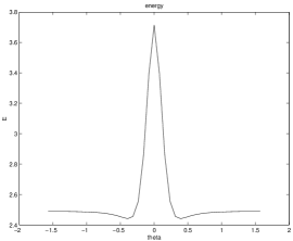
(a) Energy as function of $\theta$

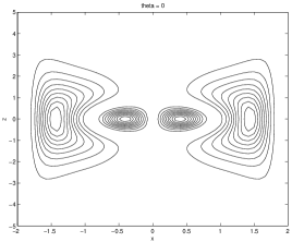
(b) $\theta=0$: rings in $xy$-plane

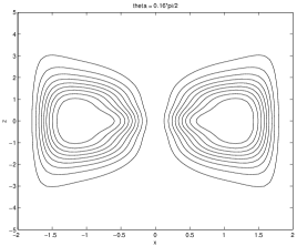
(c) $\theta=0.16\,\pi/2$: merged rings

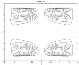
(d) $\theta=\pi/2$: separated solitons

Figure 1: A one-parameter family of soliton configurations, interpolating between a double ring in the $xy$-plane (with energy $E=3.71$) and two separated concentric solitons (with energy $E=2E_{1}=2.48$). The energy is plotted in (a), as a function of $\theta$. The other three subfigures are contour plots of $\phi^{3}$, in the $xz$-plane.

When $\theta=0$, we have two concentric rings in the $xy$-plane, as described previously (Figure 1b). As $\theta$ increases, the rings move towards each other (remaining in the $xy$-plane), and the energy decreases (steeply). The rings coalesce (Figure 1c), and then begin to separate along the $z$-axis: we now have two rings of equal radius, each in the standard configuration, at $z=\pm p$ (Figure 1d). The energy reaches a minimum (in this family) of $E=2.44$ when $\theta=0.25\,\pi/2$. As $\theta$ increases further towards $\pi/2$, the separation $2p$ increases, and the energy approaches the asymptotic value $E=2E_{1}=2\times 1.24$ of two widely-separated 1-solitons.

Let us now keep the collinear arrangement of poles, ie 

$$t_{2}=-t_{1}=S\cos\theta,\quad z_{2}=-z_{1}=S\sin\theta,\quad\lambda_{1}=\lambda_{2}=1,$$ (11)

and minimize over $S$, $\theta$ and $\lambda_{3}$. Within this three-parameter family, there is a local minimum $E=2.42$ of the energy when $S=2.6$, $\lambda_{3}=0.71$ and $\theta=\pi/2$ (so the poles all lie on the $z$-axis). This is not quite a minimum within our six-parameter family of axisymmetric solitons — the energy of the configuration generated by (11) can be reduced by increasing $t_{3}$ away from zero, which corresponds to changing the relative phase of the two co-axial solitons. However, the dependence of $E$ on $t_{3}$ is not very strong, and it is reduced by less than $1\%$; the minimum $E=2.41$ is reached when $t_{3}\approx 0.6$. The actual minimum energy in this axially-symmetric class is $E=2.26$, as noted earlier. The instanton-generated soliton configuration described above looks very similar to this static solution, but its energy is about $7\%$ too high.

4 Other two-soliton configurations

This section deals with further aspects of the two-soliton parameter space. let us begin by considering the lowest-energy solution, which is axisymmetric with $m=2$; its energy is $E=2.00$ [16, 21]. To approximate it, we use the holonomy of an appropriate rotationally-invariant instanton; this also models the minimal-energy two-Skyrmion [4, 5]. The instanton poles are chosen to have equal weights $\lambda_{a}=1$, and to lie at the vertices of an equilateral triangle in the $xy$ plane (the axis of symmetry will then be the $z$-axis). In other words, we may take $t_{a}=z_{a}=0$, and

$$x_{3}=0,\quad y_{3}=-S,\quad x_{2}=-x_{1}=\sqrt{3}\,S/2,\quad y_{2}=y_{1}=S/2,$$ (12)

where $S$ is a positive constant. The Hopf configurations corresponding to this one-parameter family of instantons resemble a ring in the $xy$-plane, with radius determined by $S$; this is where $\phi(s)=(0,0,-1)$. Because $m=2$, the locus $\phi^{-1}(0,0,1)$ actually consists of two copies of the $z$-axis, so the linking number is indeed $N=2$. When $S=1.72$, the energy of the family (12) attains a minimum value $E=2.08$, which is $4\%$ above the true minimum.

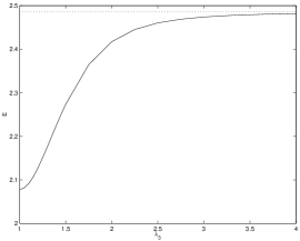
(a) Energy as function of $\lambda_{3}$

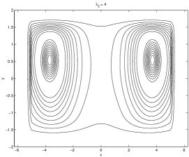
(b) $\lambda_{3}=4$: two separate solitons

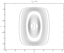
(c) $\lambda_{3}=1.15$: merging rings

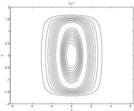
(d) $\lambda_{3}=1$: a single ring

Figure 2: A one-parameter family of soliton configurations, corresponding to two co-planar solitons attracting each other and merging to form a single $m=2$ axisymmetric configuration. The energy is plotted in (a), as a function of $\lambda_{3}$; the dotted line is the energy $2E_{1}$ of two widely-separated solitons. The other three subfigures are contour plots of $\phi^{3}$, in the $xz$-plane (the rings in (b) and (d) are circular, but look distorted because of the different scales on the two axes).

Next, consider two solitons which are far apart and co-planar (rather than co-axial as in the previous section). For appropriate orientations, they will attract each other. As the configuration moves down the energy gradient, the solitons approach each other, and the soliton rings eventually merge to form the single ring described in the previous paragraph. There is a family of instanton-generated configurations which illustrates this; the corresponding Skyrmion picture was given in [4]. We set $\lambda_{1}=\lambda_{2}=1$; the family is parametrized by $\lambda_{3}\in[1,\infty)$, with $\lambda_{3}\gg 1$ corresponding to the two solitons being far apart. The poles $X_{a}$ all lie in the $xy$-plane, so $t_{a}=z_{a}=0$. We take

$$x_{3}=0,\quad y_{3}=-S,\quad x_{2}=-x_{1}=S\cos\theta\quad y_{2}=y_{1}=S\sin\theta,$$ (13)

where $\theta$ is determined by $\sin\theta=1/(1+\lambda_{3})$; and where, for each value of $\lambda_{3}$, we find the value of $S$ which minimizes the energy $E$. Note that for $\lambda_{3}=1$, (13) reduces to (12). For $\lambda_{3}\gg 1$, the configuration consists of two rings in the $xy$-plane centred on the $x$-axis at $x\approx\pm S$; this is referred to as channel B in [21]. The results of a numerical study are summarized in Figure 2: $E$ versus $\lambda_{3}$ is given in Figure 2a, while the other subfigures provide contour plots of $\phi^{3}$ in the $xy$-plane. We see that the two individual rings join to become a single ring.

Finally, we look at a one-parameter family of configurations which interpolate between the two local minima. For this we simply rotate one into the other, by taking

$$\lambda_{1}=\lambda_{2}=1,\quad\lambda_{3}=\cos\psi+0.67\sin\psi,$$

$$t_{1}=t_{2}=-0.2\sin\psi,\quad t_{3}=0.4\sin\psi,$$

$$x_{2}=-x_{1}=1.49\cos\psi,\quad x_{3}=0,$$

$$y_{1}=y_{2}=0.86\cos\psi,\quad y_{3}=-1.72\cos\psi,$$

$$z_{2}=-z_{1}=2.55\sin\psi,\quad z_{3}=0.$$

So when $\psi=0$, we have the (global) minimum (12) with $E=2.08$; while for $\psi=\pi/2$, we have the (local) minimum described in the previous section, with $E=2.41$. The energy of the configurations in this family, as a function of $\psi$, is plotted in Figure 3.

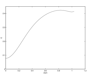
Figure 3: The energy of a family of configurations which interpolates between the global $N=2$ minimum ($\psi=0$) and the other $N=2$ minimum ($\psi=\pi/2$).

We see that there is a path between the two minima, on which the maximum energy is $E=2.43$ (which is less than twice the energy of two single solitons). In going from one minimum to the other, the curve $\phi^{-1}(0,0,-1)$ has to change from being a single ring around a double copy of the $z$-axis (when $\psi=0$) being to a pair of rings around a single copy of the $z$-axis (when $\psi=\pi/2$). So the topological behaviour of the field, as one moves along the path, is rather complicated.

5 Concluding remarks

In the case of the Skyrme model, the instanton approximation has been used to study the interaction of two Skyrmions [4, 5]; and the vibrational modes and related semiclassical quantization of the $N$-Skyrmion for $N=2$ and $N=3$ [26, 27, 28]. For higher $N$, the minimal-energy Skyrmions have the appearance of various symmetric solids (see, for example, [29, 30]), and these are quite well approximated in terms of the “rational map ansatz” [31], and variants thereof. This ansatz cannot, however, provide a full collective-coordinate manifold — its relevance is to the description of static, “superimposed” Skyrmions.

For large-$N$ Hopf solitons, one gets complicated topological structures, with evidence of many local minima (and of large changes in the field which do not change the energy much); see [18, 19, 22]. It seems unlikely that the instanton picture can capture all this structure (although it does give both the minima in the $N=2$ case). Possibly some version of the rational map ansatz might be appropriate (it was used in [18] to generate initial configurations for $N\leq 8$); but this remains an open question.

In this paper, we have seen that the “space of two Hopf solitons” can be fairly well approximated in terms of the holonomy of Yang-Mills instantons. The main application of this (as in the Skyrme case) is towards understanding the dynamics of the low-$N$ soliton systems. Hopf solitons are not spherically-symmetric — this leads to their interactions being, in some ways, more complicated than that of Skyrmions or monopoles. Much further work remains to be done towards understanding their dynamics, and the collective-coordinate description derived from instanton holonomy might be useful in that regard.

References

- [1] N S Manton, A remark on the scattering of BPS monopoles. Phys Lett B 110 (1982) 54–56.
- [2] N S Manton, Unstable manifolds and soliton dynamics. Phys Rev Lett 60 (1988) 1916–1919.
- [3] M F Atiyah and N S Manton, Skyrmions from instantons. Phys Lett B 222 (1989) 438–442.
- [4] A Hosaka, S M Griffies, M Oka and R D Amado, Two skyrmion interaction for the Atiyah-Manton ansatz. Phys Lett B 251 (1990) 1–5.
- [5] M F Atiyah and N S Manton, Geometry and kinematics of two Skyrmions. Commun Math Phys 152 (1993) 391–422.
- [6] R A Leese, N S Manton and B J Schroers, Attractive channel Skyrmions and the deuteron Nucl Phys B 442 (1995) 228–267.
- [7] R A Leese and N S Manton, Stable instanton-generated Skyrme fields with baryon numbers three and four. Nucl Phys A 572 (1995) 575.
- [8] T Ioannidou, Skyrmions from instantons. Nonlinearity 13 (2000) 1217–1225.
- [9] P M Sutcliffe, Sine-Gordon solitons from instantons. Phys Lett B 283 (1992) 85–89.
- [10] P M Sutcliffe, Kink chains from instantons on a torus. Nonlinearity 8 (1995) 411–421.
- [11] N R Cooper, “Smoke rings” in ferromagnets. Phys Rev Lett 82 (1999) 1554.
- [12] L Faddeev, Quantisation of Solitons [Preprint IAS Print-75-QS70, Princeton]; Lett Math Phys 1 (1976) 289.
- [13] A F Vakulenko and L V Kapitanskii, Stability of solitons in in the nonlinear -model. Sov Phys Dokl 24 (1979) 433–434.
- [14] A Kundu and Yu P Rybakov, Closed-vortex-type solitons with Hopf index. J Phys A 15 (1982) 269–275.
- [15] L Faddeev and A J Niemi, Stable knot-like structures in classical field theory. Nature 387 (1997) 58–61.
- [16] J Gladikowski and M Hellmund, Static solitons with nonzero Hopf number. Phys Rev D 56 (1997) 5194–5199.
- [17] R A Battye and P M Sutcliffe, To be or knot to be? Phys Rev Lett 81 (1998) 4798–4801.
- [18] R A Battye and P M Sutcliffe, Solitons, Links and Knots. Proc Roy Soc Lond A 455 (1999) 4305–4331.
- [19] J Hietarinta and P Salo, Faddeev-Hopf knots: dynamics of linked un-knots. Phys Lett B 451 (1999) 60–67.
- [20] R S Ward, Hopf solitons on and . Nonlinearity 12 (1999) 241–246.
- [21] R S Ward, The interaction of two Hopf solitons. Phys Lett B 473 (2000) 291–296.
- [22] J Hietarinta and P Salo, Ground state in the Faddeev-Skyrme model. Phys Rev D 62 (2000) 081701.
- [23] M F Atiyah, Magnetic monopoles in hyperbolic space. In: Proceedings of the International Colloquium on Vector Bundles, Tata Institute and Oxford University Press, 1984.
- [24] C Nash, Geometry of hyperbolic monopoles. J Math Phys 27 (1986) 2160–2164.
- [25] R Jackiw, C Nohl and C Rebbi, Conformal properties of pseudoparticle configurations. Phys Rev D 15 (1977) 1642–1646.
- [26] N R Walet, The kinetic energy and the geometric structure in the sector of the Skyrme model: a study using the Atiyah-Manton ansatz. Nucl Phys A 586 (1995) 649.
- [27] N R Walet, Quantising the and Skyrmion systems. Nucl Phys A 606 (1996) 429–458.
- [28] C J Houghton, Instanton vibrations of the 3-Skyrmion. Phys Rev D 60 (1999) 105003. hep-th/9905009
- [29] R A Battye and P M Sutcliffe, Solitonic fullerenes. Phys Rev Lett 86 (2001) 3989–3992. hep-th/0012215
- [30] R A Battye and P M Sutcliffe, Skyrmions, fullerenes and rational maps. hep-th/0103026
- [31] C J Houghton, N S Manton and P J Sutcliffe, Rational maps, monopoles and Skyrmions. Nucl Phys B 510 (1998) 507–537.