CU-TP-1026 , HU-EP-01/29 , UPR-950T
hep-th/0108078
Four-Dimensional $N=1$ Super Yang-Mills Theory
from an M-Theory Orbifold

Gravitational and gauge anomalies provide stringent constraints on which subset of chiral models can effectively describe M-theory at low energy. In this paper, we explicitly construct an abelian orbifold of M-theory to obtain an $N=1$, chiral super Yang-Mills theory in four dimensions, using anomaly matching to determine the entire gauge and representation structure. The model described in this paper is the simplest four dimensional model which one can construct from M-theory compactified on an abelian orbifold without freely-acting involutions. The gauge group is $SO(12)\times SU(8)\times SU(2)\times SU(2)\times U(1)$.

1 Introduction

Despite the fact that a fundamental description of M-theory has so far remained elusive, it is nevertheless possible to describe interesting and predictive aspects of its effective phenomenology. This is possible because, whatever M-theory turns out to be, it should relate at low energy to eleven-dimensional supergravity. This statement is actually quite powerful, especially when eleven-dimensional spacetime has a topology involving a compact orbifold factor, owing to rigorous constraints derivable from requirements imposed by field theory gauge and gravitational anomaly cancellation.

There has been quite a lot of recent interest in $M$-theory on $G_{2}$ holonomy seven-manifolds for the construction of $N=1$ supersymmetric theories in four dimensions [1, 2]. In this paper we describe, in microscopic detail, a particular $N=1$ model associated with a particularly interesting M-theory orbifold . Although our model involves compactification on a seven-manifold, it has the structure of a $T^{6}/(\mathbb{Z}_{2}\times\mathbb{Z}_{2})$ orbifold (admitting a Calabi-Yau resolution, [3]) times a closed interval $S^{1}/\mathbb{Z}_{2}$. Such an “orbifold with boundary” falls outside of the class of $G_{2}$-resolvable orbifolds of $T^{7}$ studied by Joyce [3] . Nevertheless, by compactification on this orbifold we do obtain a four-dimensional, $N=1$, chiral super Yang-Mills theory from eleven-dimensional supergravity via explicit cancellation of anomalies.

In our analysis, we impose strict anomaly cancelation at each point in the eleven-dimensional spacetime. This is a substantially more restrictive criterion than that implied by anomaly cancellation on smaller spaces obtained when compact dimensions shrink to zero size. The latter circumstance accesses only what we call the collective anomaly, whereas our approach involves a more “microscopic” picture of the localized states. Admittedly, in our approach we are able to compute only those chiral states needed to cancel anomalies. Any additional localized states which can be added without introducing additional anomalies are invisible to our analytic probe. Typically, this redundancy is of very limited scope, however. In this paper we describe a consistent microscopic description of the localized states in one particular orbifold. Furthermore, as explained in [6], one expects a hierachy of consistent solutions for the gauge group and representation content associated with a given orbifold compactification of M-theory. Typically, sets of such consistent solutions are linked by phase transitions, often mediated by fivebranes and small instanton transformations. In this paper we discuss only one particular solution; we fully expect that this solution describes only one corner of a more robust and interesting moduli space. Having said this, we remark that the particular M-theory orbifold analyzed in this paper had been previously mentioned in [4] as an interesting N=1 model, where it appeared as Model (C’,C’). However, in that paper no attempt was made to describe the associated spectrum from a microscopic point of view. The fact that the gauge group described in that paper differs from ours is not particulaly troubling either, since we are describing a different corner of moduli space. It would be an interesting exercise to provide a microscopic description of the models described in [4]. To the best of our knowledge this current paper is the only extant microscopic description of a $D=4$ $N=1$ model derived from M-theory.

The reason why anomaly cancellation is important in the context of M-theory orbifolds is that the the lift of the action of the orbifold quotient group to the gravitino field generically serves to project that field chirally onto even-dimensional fixed-point loci. On fixed-planes of dimensionality ten or six this projection induces gravitational anomalies, owing to the chiral coupling of the gravitino to currents which are classically conserved due to classical reparameterization invariance of the fixed-planes. However, since all local anomalies must cancel, the presence of gravitino-induced fixed-plane anomalies allows one to infer additional structure, such as Yang-Mills supermultiplets living on the fixed-planes, or specialized electric and magnetic sources of $G$ flux , since these supply necessary contributions to the overall anomaly, either quantum mechanically or as “inflow”, so as to render the theory consistent.

In generic situations orbifold fixed-point loci can be complicated, involving fixed-planes of various dimensionalities which can intersect. As a result there are additional concerns owing to gauge anomalies and mixed anomalies induced by chiral projection of the gaugino fields in the Yang-Mills supermultiplets onto fixed-plane intersections. Because of this, the cancellation of all anomalies typically involves an elaborate conspiracy of quantum contributions and inflow contributions. In a previous series of papers [5, 6, 7, 8], much of the technology needed for implementing anomaly matching in orbifolds with intersecting fixed-planes was developed. Complementary aspects and several physical observations about these orbifolds were also addresed by other authors, [9] and [10] in particular. This work extended the ideas and technology implemented in simpler orbifolds involving only isolated (i.e. non-intersecting) fixed-planes described by Hořava and Witten [11, 12] and by Dasgupta and Mukhi [13]. Until now, the only orbifolds with intersecting fixed-planes which have been analyzed are those corresponding to topologies $\mathbb{R}^{6}\times S^{1}/\mathbb{Z}_{2}\times K3$ in which the $K3$ factor degenerates to a global orbifold $K3\to T^{4}/\mathbb{Z}_{M}$, for the four possible cases $M=2,3,4$ and $6$. The effective theory in these previously studied cases, obtained in the limit that the radii of the compact dimensions becomes very small, are uniformly six-dimensional.

In this paper we describe a new example of an M-theory orbifold which has a four-dimensional effective description, and also has four dimensional fixed-planes. This model exhibits a pretty feature in that each four-dimensional fixed-plane lies at the mutual intersection of three orthogonal six-dimensional fixed-planes, each of which is a sub-manifold of a ten-dimensional fixed-plane. What is nice about this feature is that the constraints imposed by ten- and six-dimensional gravitational anomaly cancellation impinge directly on the structure of the effective field theory in four dimensions, despite the fact that there are no gravitational anomalies specifically in four dimensions. This is possible because the four-planes in question are very special sub-manifolds of the fixed ten-planes and also of the fixed six-planes. This introduces gravitational anomalies into four dimensional physics in a novel manner. Thus, despite the fact that the model which we present is not of immediate phenomenological interest, it does indroduce a powerful formalism for deriving four-dimensional physics from M-theory.

In our model, eleven-dimensional spacetime has topology $\mathbb{R}^{4}\times S^{1}/\mathbb{Z}_{2}\times T^{6}/(\mathbb{Z}_{2})^{2}$. This orbifold is of the Hořava-Witten variety, since it includes $S^{1}/\mathbb{Z}_{2}$ as a factor, and has quotient group $(\mathbb{Z}_{2})^{3}$. Since the orbifold is of the Hořava-Witten variety, in order to cancel the ten-dimensional anomaly, the fixed ten-planes, of which there are two, each support $E_{8}$ Yang-Mills supermultiplets. In this case, however, there are additional gravitational anomalies induced on the six-planes. In order to cancel these, it is necessary to introduce hypermultiplets living on these six-planes. Furthermore, it is necessary that the ten-dimensional $E_{8}$ gauge group is broken to a subgroup $E_{8}\to{\cal G}_{\alpha}\subset E_{8}$ on the six-dimensional fixed-plane corresponding to the element $\alpha$ of $(\mathbb{Z}_{2})^{3}$. This symmetry breakdown is codified by the action of the quotient group on the $E_{8}$ root lattice and is, in effect, a description of a small $E_{8}$ gauge instanton which is localized on the fixed-plane.

In our model, the cancellation of anomalies on the ten-dimensional fixed-planes and also on the six-dimensional fixed-planes proceeds exactly as described in [7] for the case of the $S^{1}/\mathbb{Z}_{2}\times T^{4}/\mathbb{Z}_{2}$ compactification. This is because these planes are locally identical to the analogs in that simpler construction. The novel feature of the $(\mathbb{Z}_{2})^{3}$ model, however, derives from the fact that the six-planes intersect each other at four-planes. As a result of this, there are important consistency requirements which control the ultimate breakdown patterns of $E_{8}$ as one approaches first a six-plane and then moves along that six plane and lands on the four plane intersection. In this paper, we present an explicit consistency analysis which enables us to compute the complete set of twisted states and the gauge group localized on the four-dimensional fixed-planes. We do not review the Hořava-Witten analysis [12] which explains the ten-dimensional anomaly cancellation nor do we review the cancellation of the six-dimensional anomalies. The interested reader is referred to [5, 6, 7, 8] for a comprehensive description of these cases.

Section 2 addresses the global geometric aspects of our model, describing the explicit action of $(\mathbb{Z}_{2})^{3}$ which gives rise to our orbifold of $T^{7}$. In the next section, the analysis of the local anomaly for the $(Z_{2})^{2}$ orbifold in [6, 7] is extended to this case. Although the story for the ten-planes is quite analogous, the six-planes require more subtle methods. For this reason we introduce “branching tables” and “embedding diagrams” for determining which projections in the $E_{8}$ root lattice are compatible with the orbifold quotient group action. In Sections 4 and 5 we use this data to determine the spectrum seen by the four-dimensional intersection which arises from the ten-dimensional $E_{8}$ fields, and discuss further twisted states which we need to introduce to cancel the six-dimensional anomalies. Finally, following a synopsis, we indicate why the four-dimensional gauge anomaly does not arise for our orbifold, and summarize the representation content of the chiral multiplets in our model (“Model 1”) in Table 7. Further models with $D=4$ and $N=1$ SUSY, based on both abelian and non-abelian orbifolds, will be discussed in forthcoming work.

2 Global Geometric Aspects

Consider a spacetime with topology $\mathbb{R}^{4}\times T^{7}$, where the compact $T^{7}$ factor is described by the quotient $\mathbb{R}^{7}/\Lambda$ with lattice $\Lambda$. Parameterize the compact dimensions using three complex coordinates $\{z_{1},z_{2},z_{3}\}$ and one real coordinate $x^{11}$. The orbifold which defines our model is obtained from this torus by making additional identifications described by parity flips as shown in Table 1. The sole condition on the lattice $\Lambda$ in $\mathbb{C}^{3}\oplus\mathbb{R}$ is that these parity flips induce lattice automorphisms. A minus sign in that table implies a relative overall sign change of the indicated coordinate (the column header) by the indicated element (the row header). Each row in Table 1 describes a generator of the full quotient group, which is $(\mathbb{Z}_{2})^{3}$.

	$z_{1}$	$z_{2}$	$z_{3}$	$x^{11}$
$\alpha$	$-$	$+$	$-$	$-$
$\beta$	$-$	$-$	$+$	$-$
$\gamma$	$+$	$-$	$-$	$-$

Table 1: The action of the quotient group $(\mathbb{Z}_{2})^{3}$ on the compact coordinates $\{z_{1},z_{2},z_{3},x^{11}\}$ corresponding to the model described in the text.

The quotient group $(\mathbb{Z}_{2})^{3}$ has order eight, with elements $\{1,\alpha,\beta,\gamma,\alpha\beta,\beta\gamma,\alpha\gamma,\alpha\beta\gamma\}$. The corresponding fixed-planes have real dimensionalities $\{11,6,6,6,7,7,7,10\}$, respectively, where we have included the four non-compact dimensions in this accounting. The $\alpha\beta\gamma$-invariant ten-planes have multiplicity two, and correspond to hypersurfaces $x^{11}=0$ and $x^{11}=\pi$. We refer to these ten-planes as $M^{10}_{1}$ and $M^{10}_{2}$, respectively.

The $\alpha$-invariant six-planes, the $\beta$-invariant six-planes and the $\gamma$-invariant six-planes each have multiplicity 32, sixteen of which are submanifolds of $M^{10}_{1}$ and sixteen of which are sub-manifolds of $M^{10}_{2}$. Within a given ten-plane $M^{10}_{i}$ there are 64 parallel four-planes which are each invariant under $\alpha$, $\beta$, and $\gamma$, each describing a mutually transversal intersection of one $\alpha$-plane, one $\beta$-plane and one $\gamma$-plane. The global geometry of the six-planes within a given ten-plane are conveniently depicted in Figure 2, where we have suppressed the $x^{11}$ dependance of the non-compact coordinates.

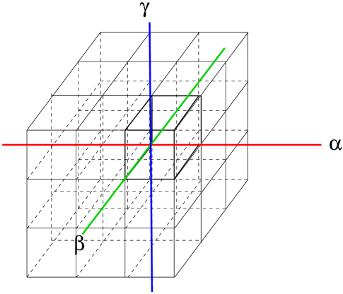
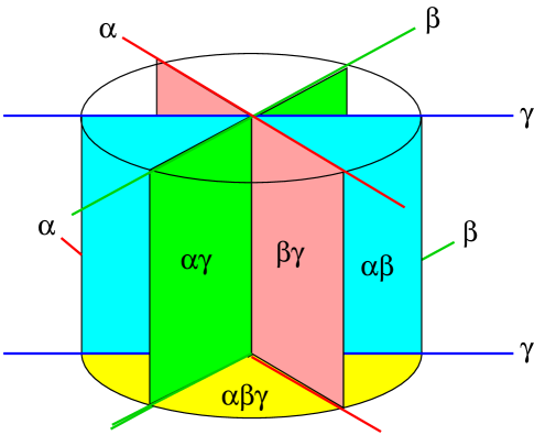
Figure 1: A depiction of the orbifold described in the text with the eleventh dimension suppressed. This picture is entirely within one of the two $\alpha\beta\gamma$ ten-planes, and illustrates the sixteen $\alpha$ six-planes, the sixteen $\beta$ six-planes and the sixteen $\gamma$ six-planes within that $\alpha\beta\gamma$ ten-plane.

Figure 2: A local depiction showing one of the sixty-four five-planes, including the eleventh dimension, and showing three of the seven planes, one each of $\alpha\beta$, $\beta\gamma$ and $\alpha\gamma$.

The $\alpha\beta$-invariant seven-planes have multiplicity sixteen. Each of these interpolates between one $\gamma$-invariant six-plane (a submanifold of $M^{10}_{1}$ ) and another $\gamma$-invariant six-plane (a submanifold of $M^{10}_{2}$), with the interpolation parameterized by $x^{11}$. Similarly, sixteen $\beta\gamma$-planes interpolate between $\alpha$-planes and sixteen more $\alpha\gamma$-planes interpolate between $\beta$-planes. The seven-planes triply intersect at 64 five-planes which are each invariant under $\alpha\beta$, $\beta\gamma$, and $\alpha\gamma$. Each five-plane interpolates between two of the four planes described above.

The global geometry is conveniently displayed as shown in Figure 2, which depicts the geometry near one of the five-planes as it interpolates between two of the four-planes. Figure 2 includes representations of every sort of fixed-plane, and every sort of intersection which occurs in this orbifold. Since the collection of planes as drawn in Figure 2 resemble a sort of waterwheel, we refer to such a diagram as a waterwheel diagram. These figures are especially useful for maintaining perspective during the ensuing analysis.

3 Local Anomaly Cancellation

As mentioned in the introduction, the geometry of the ten-planes and of the six-planes for the orbifold described in the previous section are locally identical to analogous fixed-planes in the simpler $(\mathbb{Z}_{2})^{2}$ orbifold described in [6, 7]. As a result, we can apply certain results from the analyses described in those papers. In particular, the ten-planes must each support a ten-dimensional $E_{8}$ Yang-Mills multiplet. The situation regarding the six-planes is more complicated, however. We start by reviewing the situation in the simpler $(\mathbb{Z}_{2})^{2}$ orbifold, and then describe extra constraints which pertain to the $(\mathbb{Z}_{2})^{3}$ case. For simplicity, in this paper we consider only the possibility that there are no M-fivebranes in the bulk of the orbifold.

For the case of the $S^{1}/\mathbb{Z}_{2}\times T^{4}/\mathbb{Z}_{2}$ orbifold [6, 7], we can locally cancel the six-dimensional anomalies in either of two distinct ways. In the first case a given six-plane has magnetic charge $-1/4$, while lattice reflections describe a breakdown $E_{8}\to E_{7}\times SU(2)$ as the six plane is approached. In the second case, the six-plane has magnetic charge $+1/4$ and lattice reflections describe a different breakdown $E_{8}\to SO(16)$. The ambiguity is resolved, however, by global constraints derived by integrating the $dG$ Bianchi identity. These require that the $E_{7}\times SU(2)$ solution and the $SO(16)$ solutions be paired, with one occurring on six-planes within $M^{10}_{1}$, and the other occurring in complementary six-planes inside $M^{10}_{2}$.

For the case of the $(\mathbb{Z}_{2})^{3}$ orbifold, we have three types of six-planes which respectively correspond to the elements $\alpha$, $\beta$ and $\gamma$ described above. On a given six-plane the gravitational anomaly can be cancelled locally via the same two choices described in the previous paragraph. But we need to re-think the global constraints in this context, owing to the relative complexity of the global fixed-plane network. To be concrete, we focus on the neighborhood of one of the four-dimensional intersection vertices, such as the one distinguished in Figure 2 as the intersection of the three highlighted six-planes. This same four-plane is also depicted as the upper point in Figure 2 where all of the depicted planes converge. On each of the three six-planes which mutually intersect at the given four-plane, there are two possible choices for the local gauge subgroup ${\cal G}_{i}$. Here ${\cal G}_{i}$ corresponds to ${\cal G}_{\alpha}$, ${\cal G}_{\beta}$ or ${\cal G}_{\gamma}$ depending on which six plane is being considered. In each case, the two possible choices are related to the two possible choices of magnetic charges, since these correlate with the associated $E_{8}$ lattice reflection, under which $E_{8}\to{\cal G}_{i}\subset E_{8}$.

The three six-planes being considered are all submanifolds of a particular ten-plane fixed under the triple product $\alpha\beta\gamma$. Thus, the three six-dimensional gauge groups ${\cal G}_{\alpha},{\cal G}_{\beta}$ and ${\cal G}_{\gamma}$ are each subgroups of the same $E_{8}$. These subgroups are separately fixed under the respective actions of $\alpha,\beta$, and $\gamma$ on the $E_{8}$ root lattice. An important observation is that the entire $E_{8}$ lattice must remain fixed under the triple product $\alpha\beta\gamma$. Otherwise the $E_{8}$ group would be broken at generic points on the ten-manifold, which would irreparably spoil the ten-dimensional anomaly. As a result of this, given the action of $\alpha$ and $\beta$ on the $E_{8}$ lattice, the action of $\gamma$ is fixed. Specifically $\gamma$ must act on the $E_{8}$ lattice precisely as the product $\beta^{-1}\alpha^{-1}=\alpha\beta$. (The equality follows because $\alpha$ and $\beta$ each generate $\mathbb{Z}_{2}$, and are therefore self-inverses, and because the quotient group is abelian.) This uniquely ensures that $\alpha\beta\gamma$ acts trivially on the $E_{8}$ lattice.

Subject to the constraint described in the previous paragraph, we need to determine how $\beta$ and $\gamma$ act on ${\cal G}_{\alpha}$, (i.e. how these elements are realized as reflections on the sublattice of $E_{8}$ corresponding to the root lattice of ${\cal G}_{\alpha}$), and similarly how $\alpha$ and $\gamma$ act on ${\cal G}_{\beta}$ and how $\alpha$ and $\beta$ act on ${\cal G}_{\gamma}$. Since there is a unique subgroup ${\cal H}\subset E_{8}$ which remains invariant under $\alpha$, $\beta$, and $\gamma$, it follows that the three groups ${\cal G}_{\alpha}$, ${\cal G}_{\beta}$ and ${\cal G}_{\gamma}$ must each break down to the same group ${\cal G}_{i}\to{\cal H}$ under the lattice projections described above. The state of affairs is illustrated by Figures 4 and 4.

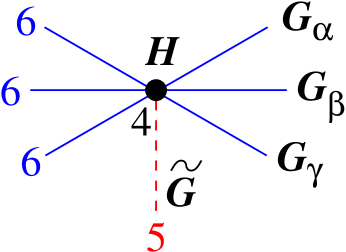
Figure 3: One of the four-dimensional intersection vertices

Figure 4: The overlapping breakdown pattern $E_{8}\to{\cal H}$

In Figure 4 we see a depiction of the three six-planes mutually intersecting at the four-plane under discussion. The four-plane is illustrated by the heavy dark spot. This figure shows the physical geometry of the fixed-plane intersection. The gauge groups corresponding to the various fixed-planes are also included in this figure, as are the dimensionalities of the planes . In Figure 4 we see a depiction of the group theoretic branchings from $E_{8}$ to the subgroup $H$, in which the consistency of the actions of the six elements of $(\mathbb{Z}_{2})^{3}$ other than the identity and the triple product $\alpha\beta\gamma$ is apparent.

We want to determine which sets of three subgroups ${\cal G}_{\alpha}$, ${\cal G}_{\beta}$ and ${\cal G}_{\gamma}$ of $E_{8}$ can consistently overlap to satisfy the situation illustrated in Figures 4 and 4. To do this, we first isolate the candidate subgroups of $E_{8}$ associated with each of the six-planes $\alpha$, $\beta$ and $\gamma$. For the case at hand, the candidate subgroups are either $E_{7}\times SU(2)$ or $SO(16)$. Thus, in this case, ${\cal G}_{\alpha}$, ${\cal G}_{\beta}$ and ${\cal G}_{\gamma}$ are each selected from between these two choices. But this must be done subject to the constraint that $\alpha\beta\gamma$ leaves the entire $E_{8}$ group invariant. This places a restriction on which combinations of selections are permitted.

There is a systematics which resolves the consistent breakdown pattern. Given a pair of subgroups ${\cal G}_{\alpha}$ and ${\cal G}_{\beta}$, we compare maximal subgroups of these to see if we can find any matches. If there is a match, then this is a candidate for the group $H$. If there aren’t any matches, then we refine the search by including subgroups at the next depth, i.e. include the maximal subgroups of maximal subgroups. For example: if we select ${\cal G}_{\alpha}=E_{7}\times SU_{2}$ and ${\cal G}_{\beta}=SO_{16}$, then there is a unique depth-one candidate for $H$, namely $SO_{12}\times SU_{2}\times SU_{2}$.

We define a preliminary breaking pattern as a set $\{\,{\cal G}_{\alpha}\,,\,{\cal G}_{\beta}\,;\,H\,\}$ meeting the above criteria. The qualifier “preliminary” reminds us that we have to verify the consistency of such an ansatz, as we explain below. Given a preliminary breaking pattern, we determine the branching pattern for the ${\bf 248}$ representation of $E_{8}$ according to $E_{8}\to{\cal G}_{\alpha}\to H$ and $E_{8}\to{\cal G}_{\beta}\to H$. For illustration, we choose $\{{\cal G}_{\alpha}\,,\,{\cal G}_{\beta}\,|\,H\,\}=\{E_{7}\times SU_{2}\,,\,SO_{16}\,|\,SO_{12}\times SU_{2}\times SU_{2}\,\}$. In this case, the $\alpha$ plane involves the following branching

$$\alpha:E_{8} \to E_{7}\times SU_{2}$$

$$\to SO_{12}\times SU_{2}\times SU_{2}$$

$${\bf 248} \to ({\bf 133},{\bf 1})\oplus({\bf 1},{\bf 3})\oplus({\bf 56},{\bf 2})$$

$$\to [\,({\bf 66},{\bf 1},{\bf 1})\oplus({\bf 1},{\bf 3},{\bf 1})\oplus({\bf 32},{\bf 2},{\bf 1})\oplus({\bf 1},{\bf 1},{\bf 3})\,]\oplus({\bf 32}^{\prime},{\bf 1},{\bf 2})\oplus({\bf 12},{\bf 2},{\bf 2})\,.$$

In this tabulation we have obtained the branching rules from [14] and/or [15]. (In the final line we have kept square brackets around the terms in the decomposition corresponding to the adjoint representation of $E_{7}\times SU_{2}$, for reasons to become apparent.) Similarly, the $\beta$ plane involves the following branching

$$\beta:E_{8} \to SO_{16}$$

$$\to SO_{12}\times SU_{2}\times SU_{2}$$

$${\bf 248} \to {\bf 120}\oplus{\bf 128}$$

$$\to [\,({\bf 66},{\bf 1},{\bf 1})\oplus({\bf 1},{\bf 3},{\bf 1})\oplus({\bf 1},{\bf 1},{\bf 3})\oplus({\bf 12},{\bf 2},{\bf 2})\,]\oplus({\bf 32},{\bf 2},{\bf 1})\oplus({\bf 32}^{\prime},{\bf 1},{\bf 2})\,,$$

where we have employed the same systematics as described above for the $\alpha$-plane branching.

We would like to express the group theoretic branching described above in terms of the orbifold quotient group acting on the $E_{8}$ root lattice. For the case at hand this is a relatively simple exercise, since all of the elements of $(\mathbb{Z}_{2})^{3}$ independently square to the identity. As a consequence, we can realize the relevant group actions as reflections on some subset of the $E_{8}$ root vectors. For example, to realize a branching $E_{8}\to E_{7}\times SU(2)$ it suffices to leave invariant 136 root vectors corresponding to roots of an $E_{7}\times SU(2)$ subgroup of $E_{8}$, and to invert the remaining 112 root vectors. Similarly to realize a branching $E_{8}\to SO(16)$ we leave invariant 120 root vectors corresponding to an $SO(16)$ subgroup and invert the remaining 128. Some of the consistency issues discussed above translate into issues pertaining to the permissible consistent choices of sublattices which can be acted upon by group elements $\alpha$, $\beta$ and $\gamma$ in particular ways.

3.1 Branching Tables

A useful tool for collecting relevant data in order to study consistent lattice projections is a special table, which we will call a “branching table”. In such a table we partition the $E_{8}$ lattice vectors, row-wise, according to representations of the subgroup $H$. We then construct three columns, one corresponding to the element $\alpha$, one to $\beta$ and one to $\gamma$. We fill out the table by placing in each slot either a plus sign or a minus sign. A plus sign indicates that the group element corresponding to the column leaves invariant those root vectors corresponding to the row. A minus sign indicates that the indicated group element reflects the associated vectors across the origin of the root space.

248	$E_{7}\times SU_{2}$	$SO_{16}$	$E_{7}\times SU_{2}$
(66,1,1)	+	+	+
(1,3,1)	+	+	+
(1,1,3)	+	+	+
(12,2,2)	$-$	$+$	$-$
(32’,1,2)	$-$	$-$	+
(32,2,1)	$+$	$-$	$-$

Table 2: Branching table describing $E_{8}\to SO_{12}\times SU_{2}\times SU_{2}$.

248	$SO_{16}$	$E_{7}\times SU_{2}$	$SO_{16}$
${\bf 63}_{0}$	+	+	+
${\bf 1}_{0}$	+	+	+
${\bf 70}_{0}$	$-$	$+$	$-$
${\bf 1}_{+2}\oplus{\bf 1}_{-2}$	$-$	$+$	$-$
${\bf 28}_{1}\oplus{\bf\overline{28}}_{-1}$	$+$	$-$	$-$
${\bf 28}_{-1}\oplus{\bf\overline{28}}_{+1}$	$-$	$-$	$+$

Table 3: Branching table describing $E_{8}\to SU_{8}\times U_{1}$.

Given the branching patterns described in (3) and (3) we construct the branching table, according to the above prescription, as shown in Table 3. The entries in the first row of Table 3 describes the way that the generator $\alpha$ acts on the $E_{8}$ root vectors, which are partitioned into representations of $H=SO(12)\times SU(2)\times SU(2)$. There are a total of 136 invariant root vectors in the first row (i.e. those with plus signs). These describe the root system of a particular $E_{7}\times SU(2)$ subgroup of $E_{8}$. This can be verified from the branching rules describing $E_{7}\to SO(12)\times SU(2)$. The second column of Table 3 corresponds to the element $\beta$. Statements analogous to those made about the first column verify that the 120 invariant vectors listed in this column describe the root system of a particular $SO(16)$ subgroup of $E_{8}$.

The third column of Table 3 describes the element $\gamma$. ¿From the discussion above, we know that this element does not act in an independent manner on the $E_{8}$ lattice. Instead, $\gamma$ acts in the same way as the product $\alpha\beta$. Thus, the third row of a given branching table, is obtained by multiplying the first column with the second column. The fact that $\{E_{7}\times SU(2),SO(16)\,|\,SO(12)\times SU(2)\times SU(2)\}$ is consistent is then verified by the fact that the action of $\gamma$ which appears in Table 3 does, in fact, reconcile as the root system of another $E_{7}\times SU(2)$ subgoup of $E_{8}$. Consistency is ensured because $E_{7}\times SU(2)$ is one of the two consistent choices of $E_{8}$ subgroups. (Consistent here means that the associated six-dimensional anomalies can be cancelled.)

In this paper we are describing a relatively simple example in which the group actions on the lattice are never more complicated than mere reflections. In future papers, however, we will describe more interesting scenarios in which the quotient group is realized relatively nontrivially on the lattices. The branching tables which we are introducing in this paper have a natural generalization in those cases.

For the consistent triple branching illustrated in Table 3, $\alpha$, $\beta$ and $\gamma$ collectively involve two branchings to $E_{7}\times SU(2)$ and one branching to $SO(16)$. Owing to global considerations discussed above, there must exist a consistent complimentary scenario, involving two instances of $SO(16)$ and one instance of $E_{7}\times SU(2)$. Since the former posibility is defined by the choice $H=SO(12)\times SU(2)\times SU(2)$, there must exist an alternate choice for $H$. Since $SO(12)\times SU(2)\times SU(2)$ was the unique common depth-one subgroup of both $E_{7}\times SU(2)$ and $SO(16)$, we need to go to greater depth in order to find an alternate preliminary breaking pattern. At the next depth there is again a unique choice, namely $\{SO(16),E_{7}\times SU(2)\,|\,SU(8)\times U(1)\}$, so that $H=SU(8)\times U(1)$. This second case can be analyzed precisely as above, with results summarized as in Table 3. (Note that it is not possible to describe a consistent triple branching involving three instances of $E_{7}\times SU(2)$ or three instances of $SO(16)$, as can be easily verified by trying to construct corresponding branching tables.)

We assume that branching decribed by Table 3 corresponds to a four-plane intersection inside of $M^{10}_{1}$, which we will call the “upstairs” region, and that the branching described by Table 3 corresponds to a four-plane intersection inside of $M^{10}_{2}$, which we will call the “downstairs” region.

3.2 Embedding Diagrams

In the “upstairs” embedding, the group ${\cal G}_{\alpha}=E_{7}\times SU_{2}$ is not the same subgroup of $E_{8}$ described by ${\cal G}_{\gamma}=E_{7}\times SU(2)$. Similarly, in the “downstairs” embedding, the group ${\cal G}_{\alpha}=SO(16)$ is not the same subgroup of $E_{8}$ described by ${\cal G}_{\gamma}=SO(16)$. The various embeddings are usefully depicted by a specialized diagram, which we will call an “embedding diagram”. These illustrate how the various groups ${\cal G}_{\alpha}$, ${\cal G}_{\beta}$, ${\cal G}_{\gamma}$ and $H$ are embedded inside of $E_{8}$, and comprise two-dimensional “maps” of $E_{8}$ in which regions denoted by closed curves correspond to specified subgroups. For instance, the “upstairs” case described by Table 3 has the embedding diagram shown in Figure 6, which we have drawn in two incarnations, side by side, with different useful aspects of data entered in each incarnation.

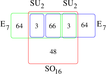
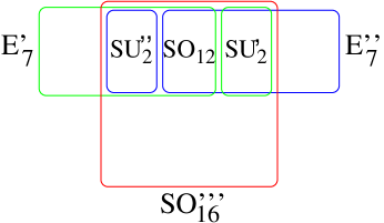
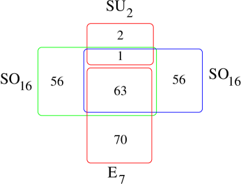
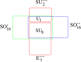
Figure 5: Embedding diagram depicting the branching $E_{8}\to SO_{12}\times SU_{2}\times SU_{2}$.

Figure 6: Embedding diagram depicting the branching $E_{8}\to SU_{8}\times U_{1}$.

In Figure 6, the subgroup ${\cal G}_{\alpha}$ is represented by the region surrounded by a green boundary, the group ${\cal G}_{\beta}$ is with a red boundary, and the group ${\cal G}_{\gamma}$ with a blue boundary. The region with a particularly colored boundary we call a bubble. Thus, the green bubble includes the 133+3=136 generators of one of the $E_{7}\times SU_{2}$ subgroups. In the left-hand diagram the dimensionalities of the subgroups are indicated and in the right-hand diagram the identity of the subgroups are indicated. Thus, the numbers in the left-hand diagram count the $E_{8}$ generators. The fact that $\alpha\beta\gamma=1$ implies restrictions which can be interpreted directly on these embedding diagrams. For instance, since each column in Table 3 must have entries whose product is plus one, it follows that there can be either three plusses and no minuses or one plus and two minuses in any column. There is no other possibility. As a result, the embedding diagram will include regions which are enclosed by all three bubbles or by only one. Furthermore, every one of the 248 generators of $E_{8}$ are enclosed in at least one bubble. These topological restrictions on the embedding diagram encapsulate the consistency requirement imposed by $\alpha\beta\gamma=1$. The “downstairs” branching, described by Table 3, is likewise described by the embedding diagram shown in Figure 6. The set of generators enclosed in all three bubbles corresponds to the group $H$. Thus, we can read from figure 6 the complete embedding of all four subgroups ${\cal G}_{\alpha}\subset E_{8}$, ${\cal G}_{\beta}\subset E_{8}$, ${\cal G}_{\gamma}\subset E_{8}$ and $H\subset E_{8}$.

4 The Four-Dimensional Spectrum

¿From the information included in the branching table and the embedding diagram, it is straightforward to determine the spectrum seen by the four-dimensional intersection which arises from the ten-dimensional $E_{8}$ fields. (We will call these the $10\to 4$ fields because of useful comparisons to be made later on.) We decompose the ten-dimensional vector fields into four-dimensional fields as $A_{\bar{\mu}}^{a}=\{A_{\mu}^{a}\,,\,\Phi_{1}^{a}\,,\,\Phi_{2}^{a}\,,\,\Phi_{3}^{a}\,\}$, where $A_{\mu}^{a}$ are four dimensional vectors and $\Phi_{i}^{a}$ are three sets of complex scalars. A given $\Phi_{i}^{a}$ combines with the four-dimensional vector to form a six-dimensional vector. Thus, $\Phi_{1}^{a}$ describes a four-dimensional scalar, but corresponds to vector degrees of freedom on the six-dimensional $\alpha$-plane (but as scalars on the $\beta$ and $\gamma$ six-planes). Similarly, $\Phi_{2}^{a}$ is associated with the $\beta$-plane and $\Phi_{3}^{a}$ is associated with the $\gamma$ plane. The three generators $\alpha$, $\beta$ and $\gamma$ act on the tensor components (i.e. the lower index) of $A_{\bar{\mu}}^{a}$ via multiplication by signs as listed in Table 4. (This describes the tensorial transformation derived from the quotient group action shown in Table 1.)

	$\alpha$	$\beta$	$\gamma$
$A_{\mu}^{a}$	$+$	$+$	$+$
$\Phi_{1}^{a}$	$-$	$-$	$+$
$\Phi_{2}^{a}$	$+$	$-$	$-$
$\Phi_{3}^{a}$	$-$	$+$	$-$

Table 4: The tensorial action of the three elements $\alpha$, $\beta$ and $\gamma$ on the components of a ten-dimensional vector field. Note: we have not included the action on the group index $a$ (i.e. the lattice action) in this table; these are described in Table 3 or 3.

The full action of the quotient group $(\mathbb{Z}_{2})^{3}$ on the $E_{8}$-valued fields $A_{\bar{\mu}}^{a}$ includes not only the tensorial action (the lower index), but also the action on the $E_{8}$ root lattice (codified by the upper index). The components of $A_{\bar{\mu}}^{a}$ partition into vector and scalar fields, but also into different representations of $H$, as tabulated in the rows of Table 3 and Table 3. Each partition transforms according to the product of the relevant entry in Table 4 with the corresponding entry in the appropriate branching table, either Table 3 or Table 3 depending on whether the four-plane is “upstairs” of “downstairs” respectively. On the four-plane the surviving components are those which transform trivially under each generator $\alpha$, $\beta$ and $\gamma$; those transforming non-trivially under any one of these are projected out. Thus, surviving fields transform with an overall plus sign under each of the generating elements $\alpha$, $\beta$ and $\gamma$, taking both the tensorial action and the $E_{8}$ lattice action together. Therefore, we resolve the $10\to 4$ spectrum by comparing Table 3 with Table 4, and matching the rows. Surviving vectors transform in representations of $H$ indicated by $(+++)$, while surviving complex scalars transform in representations indicated by $(--+)$, $(+--)$ or $(-+-)$. Surviving vectors live in $N=1$ vector supermultiplets and surviving scalars live in chiral multiplets.

The $10\to 4$ spectrum seen by an upstairs four-plane (i.e. one whose branching is described by Table 3 or by Figure 6) involves 66+3+3=72 vector multiplets transforming as the adjoint of $SO_{12}\times SU_{2}\times SU_{2}$ and 64+48+64=176 chiral multiplets transforming as

$$({\bf 32}^{\prime},{\bf 1},{\bf 2})\oplus({\bf 12},{\bf 2},{\bf 2})\oplus({\bf 32},{\bf 2},{\bf 1})\,.$$ (3)

The respective terms in this decomposition correspond to 6D scalars on the $\alpha$, $\beta$ and $\gamma$ fixed-planes. Note that the respective multipicities can also be read off of the embedding diagram from the bubbled regions outside of the total intersection.

The $10\to 4$ spectrum seen by an downstairs four-plane (i.e. one whose branching is described by Table 3 or by Figure 6) involves 63+1=64 vector multiplets transforming as the adjoint of $SU(8)\times U(1)$ and 56+56+70+2=184 chiral multiplets transforming as

$${\bf 28}_{-1}\oplus{\bf\overline{28}}_{+1}\oplus{\bf 28}_{1}\oplus{\bf\overline{28}}_{-1}\oplus{\bf 70}_{0}\oplus{\bf 1}_{+2}\oplus{\bf 1}_{-2}\,.$$ (4)

Note again that the respective multipicities can also be read off of the embedding diagram from the bubbled regions outside of the total intersection.

5 Remaining Twisted Sectors

There are two more sources of twisted matter for the orbifold which we are discusing. The first are six-dimensional fields added to some of the six-planes in order to cancel purely six-dimensional anomalies. The second are seven-dimensional fields added to the seven-planes, because these too are needed to cancel the six-dimensional anomalies. This last statement is a subtle one, which was described in [5, 6, 7] and summarized in [8]. In this section we discuss all of the remaining twisted states in this orbifold.

5.1 Six-Dimensional Fields

As described in [6, 7] the six dimensional anomaly is cancelled without six-dimensional twisted fields for the case of $E_{8}\to E_{7}\times SU(2)$ breakdown. For $E_{8}\to SO(16)$ breakdown, however, it is necessary to add six-dimensional hypermultiplets. These transform as ${\textstyle\frac{1}{2}}({\bf 16},{\bf 2})$ under $SO(16)\times SU(2)$ where the $SU(2)$ factor is associated with the adjacent seven-plane. (The extra $SU(2)$ is a subgroup of the “other” $E_{8}$ factor, as we recall in the next subsection.) The six-dimensional twisted fields reduce to chiral multiplets in four dimensions. We refer to these fields as the $6\to 4$ spectrum

For the “upstairs” four planes, only the $\beta$-invariant six-planes support the branching $E_{8}\to SO(16)$. Because of this, we add hypermultiplets transforming as ${\textstyle\frac{1}{2}}({\bf 16},{\bf 2})$ to the upstairs $\beta$-planes. The four-plane intersections see these fields as $N=1$ chiral multiplets . The representation branches to $H\times SU(2)$ according to

$$SO_{16}\times SU_{2} \to SO_{12}\times SU_{2}\times SU_{2}\times SU_{2}$$

$$({\bf 16},{\bf 2}) \to ({\bf 12},{\bf 1},{\bf 1},{\bf 2})\oplus({\bf 1},{\bf 2},{\bf 2},{\bf 2})\,;$$ (5)

the “upstairs” $6\to 4$ spectrum includes chiral multiplets transforming under $SO(12)\times SU(2)\times SU(2)$ according to the right hand side of (5).

For the “downstairs” four planes, the $\alpha$-planes and the $\gamma$-planes support $E_{8}\to SO(16)$ branchings. Because of this, we add hypermultiplets to the downstairs $\alpha$-planes and the downstairs $\gamma$-planes. In either case, the associated twisted matter branches to the four-dimensional gauge group $H\times SU(2)$ according to

$$SO_{16}\times SU_{2} \to SU(8)\times U(1)\times SU(2)$$

$$({\bf 16},{\bf 2}) \to ({\bf 8},{\bf 2})_{0}\oplus({\bf\overline{8}},{\bf 2})_{0}\,;$$ (6)

the “downstairs” $6\to 4$ spectrum includes chiral multiplets transforming under $SU(8)\times SU(2)\times U(1)$ according to the right hand side of (5). (A more precise accounting of which $SU(2)$ factors are being referred to in each case is tabulated below in Table 6, in a manner which will be explained.)

5.2 Seven-Dimensional Fields

The seven-planes corresponding to the group elements $\alpha\beta$, $\beta\gamma$ and $\alpha\gamma$ each carry vector multiplets. For the $(\mathbb{Z}_{2})^{3}$ orbifold, these each support $SU(2)$ vector multiplets. These are chirally projected on the intersecting six-planes corresponding to $\alpha$, $\beta$ and $\gamma$ onto six-dimensional hyper or vector multiplets in a way dictated by the cancellation of six-dimensional anomalies. The choice of projection onto the vectors or hypers is resolved in [6, 7] for each global abelian $S^{1}/\mathbb{Z}_{2}\times K3$ orbifold. Since the cases under discusion include these simpler cases as sub-orbifolds, this issue is already resolved. The appropriate choices are indicated by arrows in diagrams such as Figure 7, with “$V$” or “$H$” labels describing the appropriate local projection. To determine the four-dimensinal spectrum from these fields, we have to further project from six-dimensions down to four. The result is that the seven-dimensional vectors undergo a projection $7\to 6\to 4$ of one of three sorts, $V\to H\to H$, $V\to V\to V$ or $V\to V\to H$. Further details are explained in [6, 7]. This determines the so-called $7\to 4$ fields. Rather than list these here, we include these in the all-encompassing tables presented in the next section which summarize the various sectors of the effective four-dimensional spectrum.

6 Synopsis

By including $E_{8}$ Yang-Mills multiplets on the fixed ten-planes we cancel the ten dimensional anomalies. By properly accounting for the action of the $(\mathbb{Z}_{2})^{3}$ quotient group on the $E_{8}$ root lattice we can describe a consistent breakdown of these $E_{8}$ factors to appropriate subgroups on the various fixed six-planes. These are generically either $E_{7}\times SU(2)$ subgroups or $SO(16)$ subgroups. For the cases where the six-dimensional gauge group is $SO(16)$ we must include additional hypermultiplets on these six-planes. In order to cancel the six-dimensional anomalies we also include seven-dimensional $SU(2)$ Yang-Mills multiplets on the fixed seven-planes. At the same time we assign magnetic $G$ charges to the six-planes to enable the appropriate inflow anomalies. (This last part of the story has been largely suppressed in this paper because the relevant discussion found in [6, 7] is unchanged in this context, save for one global result related to this issue: that the upstairs and downstairs breaking need be complementary in sense described above.) The state of affairs is largely summarized by Figure 7.

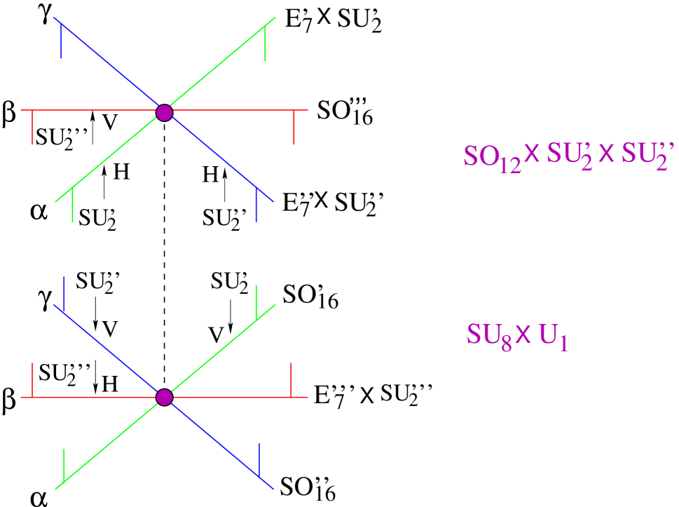
Figure 7: Synopsis

Figure 7 summarizes the juxtaposition of all of the various gauge group factors and the associated projections. This figure is a streamlined version of the waterwheel diagram shown in Figure 2, with a few lines removed and with extra data drawn in. The two purple dots in this diagram depict one “upstairs” four-plane and one “downstairs” four plane, as well as lines representing each of the six-planes which intersect at these points. The groups ${\cal G}_{\alpha}$, ${\cal G}_{\beta}$ and ${\cal G}_{\gamma}$ are indicated to the immediate right of the relevant six-planes, and the group $H$ is indicated to the far right for each of the cases, upstairs and downstairs. The orbifold consists of an aggregation of 32 regions such as the one shown in this figure.

Having reconciled all of the twisted states, be they ten, six or seven dimensional, into the four dimensional projections seen by a particular four plane, the one remaining issue is to study an additional four-dimensional anomaly which might arise due to these fields. In four dimensions, the only type of anomaly is a gauge anomaly. Generally, such will arise due to chiral coupling of the ten, six, or seven dimensional fields to the four dimensional gauge currents. If there is a four-dimensional gauge anomaly, this must be resolvable by the addition of purely four-dimensional twisted fields.

In order to determine the remaining anomaly we can use index theorems. However, this requires special care, since the index theorem results usually employed for anomaly calculations decribe anomalies due to the chiral coupling of fields with certain dimensionality to currents of that same dimensionality. As emphasized in [12] and used extensively in [5, 6, 7, 8], this is not necessarily the state of affairs in orbifolds, where the index theory results must be modified by certain divisors which are corellated with the multiplicities of fixed-planes. We have summarized the effective spectrum of twisted fields as seen by particular four-dimensional intersections, for the $(\mathbb{Z}_{2})^{3}$ orbifold, in Tables 5 and 6, where we have also included the relevant multiplicity divisor for the indicated representations. The fractions which appear in these tables, therefore, indicate the number of four-planes over which a given higher dimensional twisted state is distributed. In order to compute the effective low energy theory obtained by letting all 64 four-planes coelesce, these fractions usefully account for the appropriate multiplicities in the spectrum.

	10D	6D	7D
Chiral	${\textstyle\frac{1}{64}}({\bf 32},{\bf 2},{\bf 1},{\bf 1})$	${\textstyle\frac{1}{4}}({\bf 12},{\bf 1},{\bf 1},{\bf 2})$	${\textstyle\frac{1}{8}}({\bf 1},{\bf 3},{\bf 1},{\bf 1})$
	${\textstyle\frac{1}{64}}({\bf 12},{\bf 2},{\bf 2},{\bf 1})$	${\textstyle\frac{1}{4}}({\bf 1},{\bf 2},{\bf 2},{\bf 2})$	${\textstyle\frac{1}{8}}({\bf 1},{\bf 1},{\bf 3},{\bf 1})$
	${\textstyle\frac{1}{64}}({\bf 32^{\prime}},{\bf 1},{\bf 2},{\bf 1})$
Vector	${\textstyle\frac{1}{64}}({\bf 66},{\bf 1},{\bf 1},{\bf 1})$		${\textstyle\frac{1}{8}}({\bf 1},{\bf 1},{\bf 1},{\bf 3})$
	${\textstyle\frac{1}{64}}({\bf 1},{\bf 3},{\bf 1},{\bf 1})$
	${\textstyle\frac{1}{64}}({\bf 1},{\bf 1},{\bf 3},{\bf 1})$

Table 5: The untwisted spectrum, in terms of four-dimensional chiral multiplets and vector multiplets at one of the “upstairs” orbifold four-planes expressed in terms of representations of $SO_{12}\times SU_{2}^{\prime}\times SU_{2}^{\prime\prime}\times SU_{2}^{\prime\prime\prime}$.

	10D	6D	7D
Chiral	${\textstyle\frac{1}{64}}({\bf 28},{\bf 1},{\bf 1})_{+1}$	${\textstyle\frac{1}{4}}({\bf 8},{\bf 2},{\bf 1})_{0}$	${\textstyle\frac{1}{8}}({\bf 1},{\bf 1},{\bf 1})_{0}$
	${\textstyle\frac{1}{64}}({\bf\overline{28}},{\bf 1},{\bf 1})_{-1}$	${\textstyle\frac{1}{4}}({\bf\overline{8}},{\bf 2},{\bf 1})_{0}$	${\textstyle\frac{1}{8}}({\bf 1},{\bf 1},{\bf 1})_{+2}$
	${\textstyle\frac{1}{64}}({\bf 70},{\bf 1},{\bf 1})_{0}$	${\textstyle\frac{1}{4}}({\bf 8},{\bf 1},{\bf 2})_{0}$	${\textstyle\frac{1}{8}}({\bf 1},{\bf 1},{\bf 1})_{-2}$
	${\textstyle\frac{1}{64}}({\bf 1},{\bf 1},{\bf 1})_{-2}$	${\textstyle\frac{1}{4}}({\bf\overline{8}},{\bf 1},{\bf 2})_{0}$
	${\textstyle\frac{1}{64}}({\bf 1},{\bf 1},{\bf 1})_{+2}$
	${\textstyle\frac{1}{64}}({\bf 28},{\bf 1},{\bf 1})_{-1}$
	${\textstyle\frac{1}{64}}({\bf\overline{28}},{\bf 1},{\bf 1})_{+1}$
Vector	${\textstyle\frac{1}{64}}({\bf 63},{\bf 1},{\bf 1})_{0}$		${\textstyle\frac{1}{8}}({\bf 3},{\bf 1},{\bf 1})_{0}$
	${\textstyle\frac{1}{64}}({\bf 1},{\bf 1},{\bf 1})_{0}$		${\textstyle\frac{1}{8}}({\bf 1},{\bf 3},{\bf 1})_{0}$

Table 6: The untwisted spectrum, in terms of four-dimensional chiral multiplets and vector multiplets at one of the “downstairs” orbifold four-planes expressed in terms of representations of $SU_{8}\times SU_{2}^{\prime}\times SU_{2}^{\prime\prime}\times U_{1}$.

7 The Four-Dimensional Anomaly

It remains to study the gauge anomaly seen locally at the four dimensional intersection. In typical orbifolds, there will be a localized four-dimensional gauge anomaly. Further four-dimensional twisted states would need be added to cancel this. But in the relatively simple $(\mathbb{Z}_{2})^{3}$ orbifold described in this paper, there is no four-dimensional anomaly which needs to be cured in this way. This is because a four dimensional gauge anomaly is only generated by chiral fields transforming in complex representations. Otherwise the third index of the representation vanishes, so that ${\rm tr}\,F^{3}=0$. Since gauge anomalies in four dimensions are proportional to precisely this trace, there is no gauge anomaly induced by fields transforming in real representations. Since all of the representations which appear in Tables 5 and 6 are real, we have completed the anomaly cancellation program by adding in the ten, six and seven dimensional fields sumarized in these tables.

In the limit that the compact dimensions become very small, the effective four-dimensional spectrum is obtained by adding up the contributions from all 64 fixed four-planes. For the $(\mathbb{Z}_{2})^{3}$ orbifold the results are sumarized in Table 7.

$({\bf 32},{\bf 1},{\bf 2},{\bf 1})_{0}$	$16\,({\bf 12},{\bf 1},{\bf 1},{\bf 1})_{+1}$
$({\bf 12},{\bf 1},{\bf 2},{\bf 2})_{0}$	$16\,({\bf 12},{\bf 1},{\bf 1},{\bf 1})_{-1}$
$({\bf 32^{\prime}},{\bf 1},{\bf 1},{\bf 2})_{0}$	$16\,({\bf 1},{\bf 1},{\bf 2},{\bf 2})_{+1}$
	$16\,({\bf 1},{\bf 1},{\bf 2},{\bf 2})_{-1}$
$({\bf 1},{\bf 28},{\bf 1},{\bf 1})_{+1}$	$16\,({\bf 1},{\bf 8},{\bf 2},{\bf 1})_{0}$
$({\bf 1},{\bf\overline{28}},{\bf 1},{\bf 1})_{-1}$	$16\,({\bf 1},{\bf\overline{8}},{\bf 2},{\bf 1})_{0}$
$({\bf 1},{\bf 70},{\bf 1},{\bf 1})_{0}$	$16\,({\bf 1},{\bf 8},{\bf 1},{\bf 2})_{0}$
$({\bf 1},{\bf 1},{\bf 1},{\bf 1})_{-2}$	$16\,({\bf 1},{\bf\overline{8}},{\bf 1},{\bf 2})_{0}$
$({\bf 1},{\bf 1},{\bf 1},{\bf 1})_{+2}$
$({\bf 1},{\bf 28},{\bf 1},{\bf 1})_{-1}$
$({\bf 1},{\bf\overline{28}},{\bf 1},{\bf 1})_{+1}$

Table 7: The representation content of D=4, N=1 chiral multiplets in Model 1, in terms of the gauge group $SO_{12}\times SU_{8}\times SU_{2}\times SU_{2}\times U_{1}$. The fields above the bar arise from the upstairs sector. The fields below the bar arise from the downstairs sector. Fields with a multiplicity of 16 arise as twisted 6D fields. Note that all 7D fields cancel in the limit that all fixed-planes coalesce.

8 Conclusions

In this paper, we have shown explicitly how a four dimensional $N=1$ Yang-Mills theory can be determined from anomaly matching on the fixed-planes of an M-theory orbifold. One interesting aspect of this analysis is the manner in which constraints from gravitational anomalies impinge on the four dimensional spectrum, despite the fact that there are no gravitational anomalies in purely four dimensional field theories.

In our on-going work we are developing a systematic scan of all possible orbifolds obtained as quotients $(\mathbb{R}^{7}/\Lambda)/G$ for each possible lattice $\Lambda$ and for each possible choice of quotient group $G\subset{\rm Aut}(\Lambda)$. For a given orbifold constructed in this way we select those which have supercharges preserved on the fixed-planes, and then ascertain the fixed-plane twisted spectra needed to cancel all local anomalies. The more interesting cases involve non-abelian quotients. The orbifold described in this paper is the abelian orbifold of smallest possible group order yielding $N=1$ SUSY in four dimensions. One purpose of this paper has been to present a context for some of the rudiments of the larger algorithm which we are implementing on larger class of orbifolds, in the hopes of finding a phenomenologically compelling effective field theory limit of M-theory.

Acknowledgements
M.F. would like to thank Dieter Lüst for warm hospitality at Humboldt University where a portion of this manuscript was prepared, and also the organizers of the workshop Dualities: A Math/Physics Collaboration, ITP, Santa Barbara.

References

- [1] B.S.Acharya, On Realising N=1 Super Yang-Mills in M theory, hep-th/0011089.
- [2] M.Atiyah and E.Witten, M-Theory Dynamics on a Manifold of Holonomy, hep-th/0107177.
- [3] D.Joyce, On the Topology of Desingularizations of Calabi-Yau Orbifolds, math.AG/9806146.
- [4] R.Gopakumar and S.Mukhi, Orbifold and Orientifold Compactifications of F-Theory and M-Theory to Six and Four Dimensions, hep-th/960705.
- [5] M.Faux, D.Lüst and B.A.Ovrut, Intersecting Orbifold Planes and Local Anomaly Cancellation in M-theory, Nucl.Phys. B554 (1999) 437-483, hep-th/9903028.
- [6] M.Faux, D.Lüst and B.A.Ovrut, Local Anomaly Cancellation, M-theory Orbifolds and Phase-transitions, hep-th/0005251.
- [7] M.Faux, D.Lüst and B.A.Ovrut, An -theory Perspective on Heterotic orbifold Compactifications, hep-th/0010087.
- [8] Twisted Sectors and Chern-Simons Terms in M-Theory Orbifolds, M. Faux, D.Lust, B.A. Ovrut, hep-th/0011031.
- [9] V. Kaplunovsky, J. Sonnenschein, S. Theisen, S. Yankielowicz, On the Duality between Perturbative Heterotic Orbifolds and M-Theory on , hep-th/9912144.
- [10] Adel Bilal, Jean-Pierre Derendinger, Roger Sauser, M-Theory on : New Facts from a Careful Analysis, hep-th/9912150.
- [11] P.Hořava and E.Witten, Heterotic and Type I String Dynamics from Eleven Dimensions, Nucl.Phys. B475 (1996) 94-114, hep-th/9510209.
- [12] P.Hořava and E.Witten, Eleven-Dimensional Supergravity on a Manifold with Boundary, Nucl.Phys. B460 (1996) 506-524, hep-th/9603142.
- [13] K.Dasgupta and S.Mukhi, Orbifolds of M-theory, Nucl.Phys. B465 (1996) 399-412, hep-th/9512196.
- [14] R.Slansky, Group Theory for Unified Model Building, Phys.Rep. 79 (1981) 1-128.
- [15] W.G.McKay and J.Patera, Tables of Dimensions, Indices, and Branching Rules for Representations of Simple Lie Algebras, Marcel Dekker, Inc., 1981.