[

Semiclassical instability of the brane-world: Randall-Sundrum bubbles

Abstract

We discuss the semiclassical instability of the Randall-Sundrum brane-world model against a creation of a kind of Kaluza-Klein bubble. An example describing such a bubble space-time is constructed from the five-dimensional AdS-Schwarzschild metric. The induced geometry of the brane looks like the Einstein-Rosen bridge, which connects the positive and the negative tension branes. The bubble rapidly expands and there also form a trapped region around it.

]

In recent progress in string/M-theory, the brane-world scenario has been received much attention. This scenario gives us a new possible picture of our universe. The simplest model has been proposed by Randall and Sundrum(RS models)[1, 2]. Therein the brane consists of four-dimensional Minkowski space-time located at the boundary of the bulk five-dimensional anti-de Sitter (AdS) space-time. It can be checked that four-dimensional gravity is recovered at low energy scales on the brane [3, 4]. In addition, there are exact solutions describing the homogeneous and isotropic expanding universe [5, 6]. Unfortunately, we do not know the fundamental features of black holes so much [7, 8].

Although RS models has great success, there seems to be a crucial problem of the stability. It is well known in the standard Kaluza-Klein theory that the Kaluza-Klein vacuum is unstable against the decay channel to the so called Kaluza-Klein bubble space-time [9, 10]. Accordingly, we worry about the similar instability in RS models. This has been firstly pointed out in Ref. [11, 12](See Ref. [13] for another instability in lower dimensions.). However, the exact solution describing the Kaluza-Klein bubble space-time has not been presented in the RS brane-world context.

In this paper we will present an explicit example describing a sort of the Kaluza-Klein bubble(RS bubble) in two branes system in the RS brane-world context(RSI models). Then we show that the geometry on the brane has the structure of the Einstein-Rosen bridge [14], which connects the positive and negative tension branes. Thus the solution presented here expresses a kind of black hole in the brane-world, though it might not be what we want in the low energy scales.

The Randall-Sundrum model of single brane system (RSII)[2] is given by the metric of the form

$$g=dy^{2}+e^{-2|y|/\ell}q_{\mu\nu}dx^{\mu}dx^{\nu},$$ (1)

where $q$ is the four-dimensional Minkowski metric. The metric (1) is that of of the five-dimensional AdS space, and the brane is located at $y=0$ on which

$$K_{\mu\nu}:=\frac{1}{2}\mbox{\pounds}_{n}h_{\mu\nu}=-\frac{1}{\ell}h_{\mu\nu},$$ (2)

is satisfied, where $n=\partial_{y}$ and $h_{\mu\nu}=e^{-2|y|/\ell}q_{\mu\nu}$ is the unit normal vector and the induced metric of a $y={\rm constant}$ hypersurface. If the four-dimensional metric $q$ is replaced by a Ricci-flat metric, then Eq. (1) represents an more generic Einstein metric. Let us write the brane-metric in the form

$$q=-r^{2}d\tau^{2}+dr^{2}+r^{2}\cosh^{2}\tau d\Omega_{2}{}^{2},$$ (3)

where $d\Omega_{2}{}^{2}$ denotes the standard metric of the unit two-sphere. The metric (3) represents the Rindler space, which is locally flat, but geodesically incomplete at the null hypersurface $r=0$ (Rindler horizon). Each $r={\rm constant}$ hypersurface corresponds to the world sphere in a uniformly accelerated expansion. We here consider another generalization of Eq. (1) with a same asymptotics as Eq. (3) on the brane. This is given by

$$g = \left[\frac{1-(\rho_{*}/ar)^{2}}{1+(\rho_{*}/ar)^{2}}\right]^{2}dy^{2}+a^{2}\left[1+\left(\frac{\rho_{*}}{ar}\right)^{2}\right]^{2}(-r^{2}d\tau^{2}$$ (5)

$$+dr^{2}+r^{2}\cosh^{2}\tau d\Omega_{2}{}^{2}),$$

where $\rho_{*}>0$ is a constant and $a:=e^{-|y|/\ell}$. The metric (5) solves the five-dimensional Einstein equation with a negative cosmological term and Eq. (2) is also satisfied at every $y={\rm constant}$ hypersurface. The coordinate system used here is inappropriate at $ar=\rho_{*}$, however this is only a coordinate singularity as shown below. The metric (5) is obtained by analytic continuation of the five-dimensional AdS-Schwarzschild space-time, of which metric has the form

$$g = -F(R)dT^{2}+F(R)^{-1}dR^{2}$$ (7)

$$+R^{2}(d\chi^{2}+\sin^{2}\chi d\Omega_{2}{}^{2}),$$

$$F(R) = 1-\left(\frac{R_{*}}{R}\right)^{2}+\left(\frac{R}{\ell}\right)^{2}.$$ (8)

This metric can be analytically continued at the totally geodesic surfaces $T=0$ and $\chi=\pi/2$ by replacement of the coordinates

$$T\mapsto i\Theta,~{}~{}~{}\chi\mapsto\frac{\pi}{2}+i\tau.$$ (9)

Then the new metric becomes

$$g=F(R)d\Theta^{2}+F(R)^{-1}dR^{2}+R^{2}(-d\tau^{2}+\cosh^{2}\tau d\Omega_{2}{}^{2}),\\$$ (10)

which represents the straightforward generalization of the Kaluza-Klein bubble. The $(\Theta,R)$-plane is geodesically incomplete at

$$R=R_{h}:=\ell\left[\frac{1}{2}\left(1+\frac{4R_{*}^{2}}{\ell^{2}}\right)^{1/2}-\frac{1}{2}\right]^{1/2},$$ (11)

which can be removed by making $\Theta$ periodic with the period given by the inverse Hawking temperature: $\beta_{H}:=4\pi/F^{\prime}(R_{h})$. We shall however temporally regard the coordinate $\Theta$ as non-periodic. To arrive at the brane-world metric (5), we consider the coordinate transformation given by

$$R = ar\left[1+\left(\frac{\rho_{*}}{ar}\right)^{2}\right],$$ (12)

$$\Theta = y+\frac{1}{\ell}\int^{R}_{R_{*}}\frac{R}{F(R)}\left(1-\frac{R_{*}{}^{2}}{R^{2}}\right)^{-1/2}dR,$$ (13)

where $\rho_{*}=R_{*}/2$ and $a=e^{-y/\ell}$, and the coordinates range over $(-\infty<y<+\infty,ar>\rho_{*})$. This chart covers the region $R>R_{*}$ of the $\{\Theta,R\}$-coordinate system. If we impose the $Z_{2}$-boundary condition at $y=0$ surface, then we will obtain the brane-world model. This however is not sufficient, since $y=0$ surface is geodesically incomplete at $r=\rho_{*}$ [$(\Theta,R)=(0,R_{*})$]. This can easily be made geodesically complete by reflecting with respect to the surface $\Theta=0$; If the $y=0$ surface is given by $B_{+}$: $\{\Theta=f(R)\}$, then the reflected surface $B_{-}$: $\{\Theta=-f(R)\}$ smoothly continues to $B_{+}$ at $R=R_{*}$. We obtain the brane-world model with the brane at $B=B_{+}\cup B_{-}$ in this way (see Fig. 1).

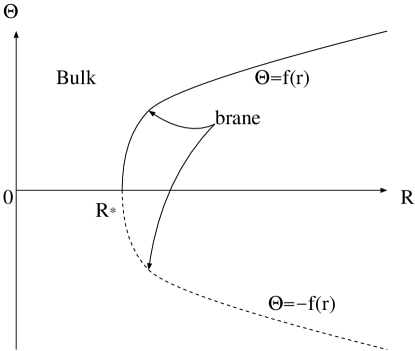
FIG. 1.: The location of a brane in $(R,\Theta)$-plane for RSII single-brane system.

However, the bulk is geodesically incomplete since it contains the point $R=R_{h}$, if a single positive tension brane is considered. Therefore, the coordinate $\Theta$ should be periodic in this case. Then, the brane intersects itself at a point given by $f(R)=\beta_{H}/2$, where a domain wall (in a four-dimensional sense) should be located. This means that the brane has a spatially compact topology, so that this is not asymptotic to the RSII model. See Ref. [15] for the similar argument in the different context.

Next, let us consider a generalization of the Randall-Sundrum model with two branes (RSI), in which a pair of branes with respective positive and negative tension is parallelly located at the boundary of the AdS bulk. In the present case, since the $(\Theta,R)$-plane is invariant under the translation in $\Theta$-direction, we can consider many copies of the brane already constructed by such a parallel translation. If the positive tension brane is given by $B=B_{+}\cup B_{-}$, the negative tension brane can be obtained by $\bar{B}=\bar{B}_{+}\cup\bar{B}_{-}$, where $\bar{B}_{\pm}$: $\{\Theta=\pm f(R)+y_{0}\}$, and $y_{0}$ denotes the separation of branes. Two branes $B$ and $\bar{B}$ intersect at $p$ given by $\Theta=y_{0}/2$; namely, two branes are connected (see Fig. 2).

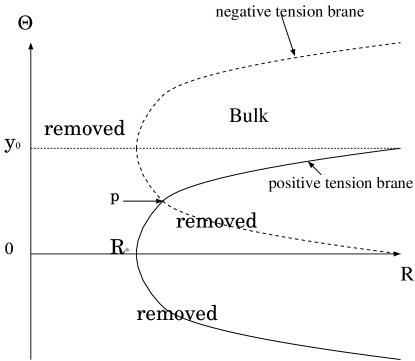
FIG. 2.: The location of branes in $(R,\Theta)$-plane for RSI two-brane system.

In the present case, we need not make $\Theta$ periodic, since the center $R=R_{h}$ can be sealed off behind the negative tension brane, so that we can obtain a brane-world model asymptotic to RSI. Note that the induced metric of the brane is smooth at $p$, where just the embedding of the boundary is singular; In fact, the intrinsic geometry of the brane constructed here is same as that of $B$ in isolation.

Here we shall consider the induced metric $h$ of the brane $B$. It can be shown that $h$ is given by

$$h=\left[1+\left(\frac{\rho_{*}}{r}\right)^{2}\right]^{2}(-r^{2}d\tau^{2}+dr^{2}+r^{2}\cosh^{2}\tau d\Omega_{2}{}^{2}).$$ (14)

The coordinate $r$ now ranges all positive value, where the region $r>\rho_{*}$ corresponds to $B_{+}$ and $0<r<\rho_{*}$ to $B_{-}$ [note that the metric (14) is invariant under $r\mapsto\rho_{*}^{2}/r$]. Let us introduce null coordinates $u_{\pm}=\tau\pm\ln(r/\rho_{*})$, then the metric (14) becomes

$$h = -\rho_{*}{}^{2}e^{u_{+}+u_{-}}\left(e^{-u_{+}}+e^{-u_{-}}\right)^{2}du_{+}du_{-}$$ (16)

$$+{\cal R}(u_{+},u_{-})^{2}d\Omega_{2}{}^{2},$$

where

$${\cal R}(u_{+},u_{-})=\frac{\rho_{*}}{2}(1+e^{u_{+}+u_{-}})(e^{-u_{+}}+e^{-u_{-}}).$$ (17)

Then, the expansion rates of the outgoing and the ingoing spherical rays are given by

$$\theta_{\pm}:=\frac{\partial\ln{\cal R}}{\partial u_{\pm}}=\frac{e^{u_{\pm}}-e^{-u_{\pm}}}{(1+e^{u_{+}+u_{-}})(e^{-u_{+}}+e^{-u_{-}})},$$ (18)

respectively. There are null hypersurfaces $H_{\pm}$

$$H_{\pm}:u_{\pm}=0$$ (19)

on which $\theta_{\pm}$ vanishes, respectively. The brane $(B,h)$ is divided by $H_{\pm}$ into four regions; (i) $I_{R}$: right asymptotic region $u_{+}>0$, $u_{-}<0$ [$(\theta_{+},\theta_{-})=(+,-)$], (ii) $I_{L}$: left asymptotic region $u_{+}<0$, $u_{-}>0$ [$(\theta_{+},\theta_{-})=(-,+)$], (iii) $T_{P}$: past trapped region $u_{+}>0$, $u_{-}>0$ [$(\theta_{+},\theta_{-})=(+,+)$], (iv) $T_{F}$: future trapped region $u_{+}<0$, $u_{-}<0$ [$(\theta_{+},\theta_{-})=(-,-)$]. The Penrose diagram is depicted in Fig. 3.

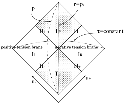
FIG. 3.: The Penrose diagram for the induced geometry of the brane corresponding to the situation in FIG. 2. The dashed line denotes the surface $p$ connecting two branes.

Each $\tau={\rm constant}$ hypersurface has the Einstein-Rosen bridge around $r=\rho_{*}$. Thus, both of the bulk and the brane has non-trivial topology (simply connected but with non-vanishing second Betti number), which represents the creation of a sort of bubbles(RS bubble). One however cannot traverse from one side to the other; Once someone steps into $T_{P}$, he will never make an exit. Thus, the region $T_{P}$ is a kind of black holes, though there is much difference from what we know of black holes. In particular, the total gravitational energy vanishes, which indicates that the RSI model might decay by creating RS bubbles semiclassically. A creation of a bubble implies a cross-linking of two branes through a topology changing process of the bulk and the brane. There is negative energy distribution around the RS bubble, which comes from the electric part of the five-dimensional Weyl tensor

$$E_{\mu\nu}={}^{(5)}C_{\mu\alpha\nu\beta}n^{\alpha}n^{\beta}$$ (20)

through the effective Einstein equation on the brane[4]

$${}^{(4)}G_{\mu}^{\nu}=-E_{\mu}^{\nu}=\frac{4\rho_{*}^{2}r^{4}}{(r^{2}+\rho_{*}^{2})^{4}}(\delta^{\tau}_{\mu}\delta^{\nu}_{\tau}-3\delta^{r}_{\mu}\delta^{\nu}_{r}+\delta_{\mu}^{\vartheta}\delta^{\nu}_{\vartheta}+\delta_{\mu}^{\varphi}\delta^{\nu}_{\varphi}).$$ (21)

The energy density observed by $r={\rm constant}$ observer therefore becomes

$$\epsilon=-\frac{\rho_{*}^{2}r^{4}}{2\pi G_{4}(r^{2}+\rho_{*}^{2})^{4}}<0,$$ (22)

of which amplitude peaks at $r=\rho_{*}$ with $|\epsilon|=(32\pi G_{4}\rho_{*}^{2})^{-1}$, and rapidly dumps as $1/r^{4}$ $(r\rightarrow+\infty)$.

Finally, we shall estimate the semiclassical decay probability of the RSI brane-world using the euclidean path integral. The corresponding euclidean bounce solution is obtained by the Wick rotation, $\tau\to i\tau_{E}+\pi/2$, of the metric of Eq (5). The decay occurs at $\tau=0$ because the 4-dimensional surfaces at $\tau=0$ is momentary static. As a result the decay probability will be order $P\sim\exp(-\frac{\ell\rho_{*}^{2}}{G_{5}})$. In the above $G_{5}$ is the five-dimensional gravitational constant having the relation with the four-dimensional gravitational constant, $G_{4}$, as $G_{5}\sim\ell G_{4}e^{2y_{0}/\ell}$. $y_{0}$ is the typical coordinate distance between two branes. In the RSI models we often assume $G_{5}\sim 1{\rm TeV}^{-3}$ and $\ell\sim 1{\rm mm}$. For $\rho_{*}>(G_{5}/\ell)^{1/2}\sim(10^{11}{\rm GeV})^{-1}$, this decay process might be suppressed.

Let us summarise our study. We presented an explicit example describing the brane-world after the Randall-Sundrum models decays. We called this the Randall-Sundrum bubble spacetimes. The brane geometry has the structure of the Einstein-Rosen bridge, but not black hole due to the negative effective energy from the bulk Weyl tensor. It turns out that RSI-type models is realised in the present procedure, but RSII type models is not. The decay probability of RSI models to RS bubble spacetimes was roughly evaluated and we saw that the decay process crucially affects the RSI brane-world scenario. Supersymmetry may be important so that it might forbid this decay process in the brane-world context as well as in the standard Kaluza-Klein theory [9].

REFERENCES

- [1] L. Randall and R. Sundrum, Phys. Rev. Lett. 83, 3370 (1999).
- [2] L. Randall and R. Sundrum, Phys. Rev. Lett. 83, 4690 (1999).
- [3] J. Garriga and T. Tanaka, Phys. Rev. Lett. 84, 2778 (2000); S. B. Giddings, E. Katz, and L. Randall, JHEP 0003, 023(2000).
- [4] T. Shiromizu, K. Maeda, M. Sasaki, Phys. Rev. D62 024012 (2000).
- [5] P. Binétruy, C. Deffayet, U. Ellwanger and D. Langlois, Phys. Lett. B477, 285 (2000); P. Kraus, JHEP 9912, 011 (1999); D. Ida, JHEP 0009, 014 (2000); S. Mukohyama, Phys. Lett. B473, 241 (2000); S. Mukohyama, T. Shiromizu and K. Maeda, Phys. Rev. D62, 024028 (2000).
- [6] J. Garriga and M. Sasaki, Phys. Rev. D62, 043523 (2000).
- [7] A. Chamblin, S. W. Hawking and H. S. Reall, Phys. Rev. D61, 065007 (2000).
- [8] R. Emparan, G. T. Horowitz and R. C. Myers, JHEP 0001,007 (2000); JHEP 0001,021 (2000); N. Dadhich, R. Maartens, P. Papadopoulos and V. Rezania, Phys. Lett. B487,1 (2000); T. Shiromizu and M. Shibata, Phys. Rev. D62, 127502 (2000); A. Chamblin, H. S. Reall, H. Shinkai and T. Shiromizu, Phys. Rev. D63, 064015 (2001); C. Germani and R. Maartens, hep-th/0107011.
- [9] E. Witten, Nucl. Phys. B195, 481 (1982).
- [10] D. Brill and H. Pfisher, Phys. Lett. B228, 359 (1989); D. Brill and G. T. Horowitz, Phys. Lett. B262, 437 (1991).
- [11] H. Shinkai and T. Shiromizu, Phys. Rev. D62, 024010 (2000).
- [12] M. Fabinger and P. Horava, Nucl. Phys. B580, 243 (2000).
- [13] D. Marolf and M. Trodden, hep-th/0102135.
- [14] A. Einstein and N. Rosen, Phys. Rev. 48, 73 (1935).
- [15] R. Gregory and A. Padilla, hep-th/0104262; hep-th/0107108.