A thick shell Casimir effect

Abstract

We consider the Casimir energy of a thick dielectric-diamagnetic shell under a uniform velocity light condition, as a function of the radii and the permeabilities. We show that there is a range of parameters in which the stress on the outer shell is inward, and a range where the stress on the outer shell is outward. We examine the possibility of obtaining an energetically stable configuration of a thick shell made of a material with a fixed volume.

1 Introduction

It is well known that the fluctuations of electromagnetic fields in vacuum or in material media depend on the boundary conditions imposed on the fields. This dependence gives rise to forces which are known as Casimir forces, acting on the boundaries. The best known example for such forces is the attractive force experienced by parallel conducting plates in vacuum [1]. Casimir forces between similar, disjoint objects such as two conducting or dielectric bodies are known in most cases to be attractive [2] and are sometimes viewed as the macroscopic consequence of Van der Waals and Casimir-Polder attraction between molecules.

However, Boyer [3] showed that the zero point electromagnetic pressure on a conducting shell is directed outward. In this paper we address the question: can there exist a compact ball for which the Casimir forces would not expand the ball to infinity? We look for such behavior in a simple model.

In view of the dominance of the Casimir forces at the nanometer scale, where the attractive force could lead to restrictive limits on nanodevices, the study of repelling Casimir forces is of increasing interest. Indeed, Boyer, following Casimir’s suggestion, studied inter plane Casimir force with one plate a perfect conductor while the other is infinitely permeable. He showed that, in this case the plates repel [4]. This problem was reconsidered since in [5, 6].

In addition to the Casimir effect for a conducting spherical shell, various cases of material balls where considered in the literature. The case of a ball made of a dielectric material was considered by many authors and exhibits strong dependence on cutoff parameters [7, 8, 9, 10, 11, 12]. The case of a dielectric-diamagnetic ball has also been extensively studied, especially under the condition of $\epsilon\mu=1$, which will be referred to as the uvl (uniform velocity of light) condition, since its introduction by Brevik and Kolbenstvedt [13, 14, 15, 16]. A medium with the uvl property has in many cases cutoff-independent values for the Casimir energy (see also [17, 18, 19] for the Casimir energy of a cylinder with uvl). A heuristic argument for this statement goes as follows: the zero point energy of the electromagnetic field in a uvl medium is a sum over the eigenfrequencies of the system, and behaves for high frequencies as $\sum_{I}\omega_{I}\sim\sum_{I}ck_{I}$, where the factor $c$ is common to all the media and the geometric information on the system enters via the allowed $k^{\prime}$s. This expression in the limit of high $k^{\prime}s$ behaves exactly as the vacuum energy with $\epsilon\mu=c^{-2}$ and the sum becomes regularizable by subtraction of the vacuum energy. In cases where this condition is not fulfilled there are problems of UV divergent terms which are proportional to the volume in which the velocity of light is different from the velocity of light in the background.

We will use the uvl condition for our thick shell.

In all of the above mentioned cases, namely, the conducting sphere, dielectric ball or a dielectric-diamagnetic ball with uvl, the resultant pressure was found to be repulsive.

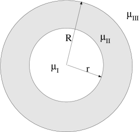
Figure 1: A thick dielectric-diamagnetic shell.

In order to obtain diverse behaviors we mix the case of disjoint bodies (where there is usually attraction) and the dielectric ball scenario as follows: We consider the case of a thick shell (fig. 1), with three permeability regimes (inner, middle and outer) $\mu_{I},\mu_{II},\mu_{III}$, under a uvl condition. In this case there are two competing effects, i.e.: interaction between the inner and outer boundaries, and the repulsive pressure experienced by each boundary.

Using a formula derived in [20] we show in sections 2 and 3 that for a dilute medium the energy of the thick shell is

$$E_{C}(r,R)=\frac{5}{128\pi R}\kappa_{R}^{2}+\kappa_{r}\kappa_{R}\frac{r^{3}(r^{2}-5R^{2})}{4(r-R)^{3}(r+R)^{3}\pi}+\kappa_{r}^{2}\frac{5}{128\pi r}$$

Where $r$ and $R$ are the inner and outer radii respectively and the parameters $\kappa_{r}$ and $\kappa_{R}$ are defined in section 3. From this expression one can easily obtain the energy of a single ball by taking the limit of $R$ to infinity, and also the energy of two parallel infinite dielectrics by taking both of the radii to infinity while keeping a finite distance $d=R-r$.

Next, in sections 4 and 5 we investigate this expression for the energy and show that there is a range of parameters such that the force on the outer shell is attractive.

2 Energy of the electromagnetic fluctuations

In this section we briefly review the Green’s function method for calculation of Casimir energies (see [21] and [20] for details). To calculate the Casimir energy of a medium under the uvl condition, we use the perturbative technique suggested in [20]. There, the Born series for the correlation function $D_{ik}(\omega;{\bf r},{\bf r^{\prime}})$ of the electromagnetic fields in material medium is presented. The correlation function $D_{ik}$ is defined by

$$D_{ik}(\omega;{\bf r},{\bf r^{\prime}})=\int_{0}^{\infty}e^{i\omega t}D^{R}_{ik}(t;{\bf r},{\bf r^{\prime}}){\rm d}t$$ (1)

where

$$D^{R}_{ik}(t_{2}-t_{1};{\bf r},{\bf r^{\prime}})=\Big{\{}\begin{array}[]{ll}i<A_{i}({\bf r},t_{1})A_{k}({\bf r^{\prime}},t_{2})-A_{k}({\bf r^{\prime}},t_{2})A_{i}({\bf r},t_{1})>&t_{1}<t_{2}\\ 0&{\rm otherwise}\end{array}$$

is the retarded Green’s function. Throughout we use the gauge $A_{0}=0$, so that the indices $i,k$ range $1,2,3$ and $D$ is a $3\times 3$ matrix.

The correlation function $D$ is known [21] to be the Green’s function for the equation (in units where $\hbar=c=1$)

$$([{\bf\nabla}]\mu^{-1}[{\bf\nabla}]-\omega^{2}\epsilon)D=-{\bf{\mathbb{I}}}$$ (2)

where $[a]$ stands for a matrix whose elements are $[a]_{ik}=\epsilon_{ijk}a_{j}$ and ${\bf{\mathbb{I}}}$ is the identity operator, which, in coordinate space is just the $3\times 3$ identity matrix times a delta function. In eq. (2), $\epsilon$ is the permittivity and $\mu$ the permeability of the medium. In the following we assume that $\mu({\bf r})$ and $\epsilon({\bf r})$ are scalar functions (of course, in the general case both $\mu$ and $\epsilon$ are tensors). This equation can be also written in the form:

$$([{\bf\nabla}]^{2}-[{\bf\nabla}\log\mu][{\bf\nabla}]-\omega^{2}\epsilon\mu)D=-\mu{\bf{\mathbb{I}}}$$ (3)

The correlation function of electromagnetic fields in vacuum, where $\epsilon=\mu\equiv 1$, will be denoted $D_{0}$. It is the inverse of the operator $([{\bf\nabla}]^{2}-\omega^{2})$ and is well known. It is given by the formula:

$$D_{0}(\omega;r,r^{\prime})=-\left({\mathbb{I}}+{1\over\omega^{2}}{\bf\nabla}\otimes{\bf\nabla}\right){1\over 4\pi|{\bf r}-{\bf r}^{\prime}|}\exp^{(i\omega|{\bf r}-{\bf r}^{\prime}|)},$$ (4)

We now wish to use the known $D_{0}$ to express $D$ via a Born series. Define:

$${\mathcal{P}}=\omega^{2}{\bf{\mathbb{I}}}(1-\mu\epsilon)$$ (5)

and

$${\mathcal{Q}}=-[{\bf\nabla}\log(\mu)][{\bf\nabla}]$$ (6)

It follows from (3) that as an operator $D$ satisfies:

$$D=((I-({\mathcal{P}}+{\mathcal{Q}})D_{0}){D_{0}}^{-1})^{-1}\mu=D_{0}(I-({\mathcal{P}}+{\mathcal{Q}})D_{0})^{-1}\mu,$$ (7)

Thus $D$ is given by the following formal series:

$$D=D_{0}\mu+D_{0}({\mathcal{P}}+{\mathcal{Q}})D_{0}\mu+D_{0}({\mathcal{P}}+{\mathcal{Q}})D_{0}({\mathcal{P}}+{\mathcal{Q}})D_{0}\mu+....$$ (8)

We now impose the ”uniform velocity of light” condition in the medium by setting $\epsilon\mu\equiv{\bf\rm I}$. This eliminates the ${\mathcal{P}}$ terms and we are left with the expansion:

$$D=D_{0}\mu+D_{0}{\mathcal{Q}}D_{0}\mu+D_{0}{\mathcal{Q}}D_{0}{\mathcal{Q}}D_{0}\mu+....$$ (9)

The correlation function $D$ can be used to calculate various properties of the electromagnetic field. We use it to calculate the energy density of the field by using the relations:

$$(E_{i}E_{k})_{\omega}=\omega^{2}(A_{i}A_{k})_{\omega}$$

and

$$(B_{i}B_{k})_{\omega}=\overrightarrow{{\bf\nabla}}\times(A_{i}A_{k})_{\omega}\times\overleftarrow{{\bf\nabla}},$$

Where the round brackets stand for the Fourier transform with respect to time of the correlation function ${1\over 2}<A_{i}({\bf r},t)A_{k}({\bf r^{\prime}},0)+A_{k}({\bf r^{\prime}},0)A_{i}({\bf r},t)>.$

At a temperature $T={1\over\beta}$ this correlation function of the fields $A_{i}$ is related to the retarded Green’s function $D$ by the fluctuation dissipation theorem [21]:

$$(A_{i}({\bf r})A_{j}({\bf r}^{\prime}))_{\omega}=-i4\pi\coth({\beta\omega\over 2})(D_{ij}({\bf r},{\bf r}^{\prime})-\overline{D_{ji}}({\bf r}^{\prime},{\bf r}))$$ (10)

Thus, at zero temperature, the energy density of the electromagnetic field is:

$$\rho({\bf r},\omega)={1\over 4\pi}\Big{(}\epsilon({\bf r})(E({\bf r})^{2})_{\omega}+{1\over\mu({\bf r})}(B({\bf r})^{2})_{\omega}\Big{)}{{\rm d}\omega\over 2\pi}=$$ (11)

$${1\over 4\pi}\lim_{{\bf r}^{\prime}\rightarrow{\bf r}}{\bf\rm Im}\,{\rm Tr}\Big{(}\omega^{2}\epsilon({\bf r})D({\bf r},{\bf r}^{\prime})+{1\over\mu({\bf r})}\overrightarrow{{\bf\nabla}}\times D\times\overleftarrow{{\bf\nabla}}\Big{)}{\rm d}\omega,$$

where we have chosen to neglect the dependence of the permeability $\mu$ and permittivity $\epsilon$ on the frequency $\omega$. Inserting the expansion (9) in (11) one can obtain a series for the energy density of fluctuations of the electromagnetic field. It was shown in [20] that the first contribution to the Casimir energy density (i.e., energy of the electromagnetic field in the presence of external conditions minus the energy density of the electromagnetic field without them) comes from the term $D_{0}{\mathcal{Q}}D_{0}{\mathcal{Q}}D_{0}\mu$ in (9) . For a dilute medium this term gives the dominant contribution to the Casimir energy.

3 Casimir energy of a thick shell

The Casimir energy per ${\rm d}\omega$ is obtained via eq. (11) by the integration of $\rho({\bf r},\omega)-({\rm contribution\,of}\,D_{0})$ over space. This yields the following general formula for the density of Casimir energy of a medium with a radially symmetric permeability $\mu$ [20] assuming the uvl property, and diluteness:

$${\rho_{T}}^{(2)}(\omega)=-4\pi\omega^{2}\coth({\beta\omega\over 2}){\rm Im}\int_{0}^{\infty}{\rm d}sI(s)(\log\mu(s))^{\prime}$$ (12)

Where:

$$I(s)=\int_{\cal T}{\rm dudv}{(u^{4}-(v^{2}-s^{2})^{2})\over 2u}g_{2}(u)(\log\mu(v))^{\prime}$$ (13)

and the integration domain ${\cal T}$ is such that $u$, $v$ and $s$ can form a triangle. The function $g_{2}$ is given by:

$$g_{2}(s)={e^{2i\omega s}\over 32\pi^{2}s}\big{(}{1\over s}-i\omega\big{)}$$ (14)

We consider a shell of thickness $R-r$ with inner radius $r$, and an outer radius $R$. The permeability of the shell is $\mu_{II}$ (Fig. 1), it is imbedded in a medium with permeability $\mu_{III}$ and its core has permeability $\mu_{I}$. We define $\kappa_{r}=\log{\mu_{I}\over\mu_{II}}$ and $\kappa_{R}=\log{\mu_{II}\over\mu_{III}}$.

We now calculate the Casimir energy of the thick shell using eq. (12). In our case $\mu$ is a sum of two radial step functions, and $\mu^{\prime}(s)$ is just a pair of delta functions at $s=r$ and $s=R$. Thus the integration over $s$ in (12) becomes immediate and yields the energy density

$${\rho_{T}}^{(2)}(\omega)=-4\pi\omega^{2}\coth({\beta\omega\over 2}){\rm Im}\left(\kappa_{r}I(r)+\kappa_{R}I(R)\right)$$ (15)

The $I$’s in (15) can be explicitly calculated:

$$I(r)=\kappa_{r}\int_{0}^{2r}{u^{3}\over 2}g_{2}(u)+\kappa_{R}\int_{R-r}^{R+r}{(u^{4}-(R^{2}-r^{2})^{2})\over 2u}g_{2}(u)$$ (16)

and:

$$I(R)=\kappa_{R}\int_{0}^{2R}{u^{3}\over 2}g_{2}(u)+\kappa_{r}\int_{R-r}^{R+r}{(u^{4}-(R^{2}-r^{2})^{2})\over 2u}g_{2}(u)$$ (17)

So that

$${\rho_{T}}^{(2)}(\omega)=-4\pi\omega^{2}\coth({\beta\omega\over 2}){\rm Im}\big{(}\kappa_{r}^{2}\int_{0}^{2r}{u^{3}\over 2}g_{2}(u)+$$ (18)

$$\kappa_{R}^{2}\int_{0}^{2R}{u^{3}\over 2}g_{2}(u)+2\kappa_{r}\kappa_{R}\int_{R-r}^{R+r}{(u^{4}-(R^{2}-r^{2})^{2})\over 2u}g_{2}(u)\big{)}$$

We can identify the first two terms as the densities of Casimir energy per ${\rm d}\omega$ for balls of radii $r$ and $R$. The total Casimir energy can now be obtained by integration of the density (18) over the frequencies $\omega$ using (26) and (27). The result is:

$$E_{C}(r,R)=\frac{5}{128\pi R}\kappa_{R}^{2}+\kappa_{r}\kappa_{R}\frac{r^{3}(r^{2}-5R^{2})}{4(r-R)^{3}(r+R)^{3}\pi}+\kappa_{r}^{2}\frac{5}{128\pi r}$$ (19)

This is our final expression for the energy of a thick shell, where the assumption of diluteness implies $|\kappa_{r}|,|\kappa_{R}|<<1$.

Let us check that this result coincides with the known result for a single sphere when $R$ goes to infinity. To do so we expand $\kappa_{r}$ in terms of the diluteness parameter $\xi={\mu_{I}-\mu_{II}\over\mu_{I}+\mu_{II}}$ which is commonly used in the literature:

$$\kappa_{r}=\log{\mu_{I}\over\mu_{II}}=\log{1-\xi\over 1+\xi}=-2\xi-2{\xi^{3}\over 3}+...$$ (20)

Substituting this expansion in (19) and taking the limit $R\rightarrow\infty$ we immediately regain the usual result for the energy of a dielectric-diamagnetic ball [16, 22], namely: $E_{C}(r,\infty)=\frac{5\,\xi^{2}}{32r\pi}+{\cal O}(\xi^{4})$. This energy yields an outward pressure on the ball.

Note also that the Casimir energy of two parallel dielectrics per unit area can be obtained from (19), by taking the limit of large radii. To see this we keep $d=R-r$ finite while taking the limit $r,R\rightarrow\infty$, and divide by the surface area thus obtaining:

$$E_{C}(d)=\frac{\kappa_{r}\kappa_{R}}{8\pi^{2}d^{3}}$$ (21)

To illustrate the broad range of behaviors that are possible from an expression for the energy such as (19), we study in more detail two cases:

1. $\kappa_{r}=-\kappa_{R}$. This happens when the inner and outer material are the same. E.g. one can imagine a thick material shell in vacuum.

2. $\kappa_{r}=\kappa_{R}$. In this case the ration of magnetic constants between the inner and middle materials is the same as the ratio between the middle and outer material.

4 Stress

Now we use the expression for the energy (19) in order to evaluate the Casimir stress on the shells. The pressure on the outer shell is given by

$${\cal F}_{R}=-{1\over 4\pi R^{2}}{\partial\over\partial R}E_{C}={1\over 4\pi^{2}R^{2}}\Big{(}{r^{3}R(r^{2}+5R^{2})\kappa_{r}\kappa_{R}\over(r-R)^{4}(r+R)^{4}}+{5\kappa_{R}^{2}\over 128R^{2}}\Big{)}$$ (22)

While the pressure on the inner shell is given by

$${\cal F}_{r}=-{1\over 4\pi^{2}r^{2}}{\partial\over\partial r}E_{C}={1\over 4\pi^{2}r^{2}}\Big{(}{r^{2}(r^{4}-10r^{2}R^{2}-15R^{4})\kappa_{r}\kappa_{R}\over 4(r-R)^{4}(r+R)^{4}}+{5\kappa_{r}^{2}\over 128r^{2}}\Big{)}$$ (23)

One may recognize the self Casimir force acting on the inner and outer shells in the terms independent of $r$ or $R$ respectively. We now turn to examine two cases:

4.1 $\kappa_{r}=-\kappa_{R}$

The pressure on the outer shell is

$${\cal F}_{R}={\kappa_{R}^{2}\over 4\pi^{2}R^{2}}\Big{(}{5\over 128R^{2}}-{r^{3}R(r^{2}+5R^{2})\over(r-R)^{4}(r+R)^{4}}\Big{)}$$ (24)

The sign of this expression depends only on the ratio $c={r\over R}$. The pressure can be written in the form:

$${\cal F}_{R}={\kappa_{R}^{2}\over 4\pi^{2}R^{2}}\Big{(}{5\over 128}-{c^{3}(c^{2}+5)\over(c-1)^{4}(c+1)^{4}}\Big{)}\,\,\,\,\,\,\,0<c<1$$ (25)

force.eps

Figure 2: Pressure on outer shell as function of the radii ratio. The Casimir force changes direction at ${r\over R}\sim 0.19$

For a constant outer radius $R$, the behavior of the pressure as a function of the ratio $c$ is indicated in Fig.2. One can see that at a radii ratio of approximately 0.19 the Casimir pressure suddenly changes sign and becomes an inward pressure. However, the pressure on the inner shell is always directed outward so that the inner and outer regions attract. This attraction may be balanced by adding the compression resistance of the middle medium, or by adding the volume dependence of $\mu$. In the case that $r<0.19R$, the pressure on the inner shell is larger than the pressure on the outer shell, so that one can imagine the two shells growing until they reach the $0.19$ ratio and then the outer shell will start contracting.

This result is not too surprising. If one considers two conducting shells which are very close, then there will be attraction between the shells, of the order of magnitude of attraction between conducting plates. This attraction will lose its dominance once the radii become far in magnitude and then each shell will experience its own outward Casimir pressure. However, in order to know if the outer radius stays finite or goes to infinity, it is necessary to introduce the law by which the smaller radius changes as we change the outer radius. An example for such a situation is given in the next section.

4.2 $\kappa_{r}=\kappa_{R}$

In this case the pressure on the outer shell is outward for all $R$. The inner shell will be subject to an outward pressure as long as $R>3.46r$. For $R<3.46r$ the pressure will be an inward one on the inner shell. We return to this situation in the next section.

5 A thick shell with a fixed volume

In the previous section we calculated the pressure assuming that the volume of the inner ball is fixed. Another interesting model is to consider the volume of the thick shell itself as constant. Thus we can assume $v={4\pi\over 3}(R^{3}-r^{3})$ remains constant, and look for a minimum of the energy under this condition.

In this case, as the outer shell expands, the distance between the inner and outer boundaries decreases. So that if there is attraction between the shells, it will be energetically favorable for the shell to expand to infinity gaining from the energy of interaction between the boundaries as well as from the tendency of each separate boundary to grow. This is indeed what happens in the case where $\kappa_{r}=-\kappa_{R}$.

However, for the second possibility, namely $\kappa_{r}=\kappa_{R}$ there is repulsion between the boundaries. This protects the shell from growing to infinity and a stable minimum of the potential can be found. A typical example is illustrated in fig. 3, where the minimum of the potential is for $R\simeq 1.01$, $r\simeq 0.31$ assuming the volume of the substance in the middle region is kept constant at ${4\pi\over 3}$.

Another possibility is to keep the distance between the shells constant (imagine the inner and outer boundaries are attached by means of stiff rods of constant length). Qualitatively the results are then similar to the results discussed above for the cases $\kappa_{r}=-\kappa_{R}$ and $\kappa_{r}=\kappa_{R}$.

pmin.eps

Figure 3: The potential of a thick shell with a fixed volume as function of $R$, for $\kappa_{r}=\kappa_{R}$. There is a clear minimum at $R=1.01$.

6 Discussion

One of the most intriguing aspects of the Casimir force is its sign: this force was shown to exhibit different behavior in different problems. It seems that the sign of the force depends on the balancing of several effects, such as a tendency to minimize the average curvature of the boundaries, and on the other hand the interaction between different patches of the boundary. In the calculations here, which are confined to the case of uniform velocity of light, we have shown how these effects can work with or against each other in an explicit way resulting in a new range of behaviors. We obtained a general expression for the energy as function of the radii and permeabilities in the limit of dilute media. In particular, for fixed distance between the shells, in the limit of radii approaching to infinity, we regain, in essence, the standard expression for the Casimir energy between parallel dielectric media. However, now the sign of the interaction energy in (19) is determined by the relative size of their permeabilities: for a shell enclosed between two vacuua we get attraction between the boundaries, as it should be for the standard Casimir two plates case. Repulsion is obtained when the permeability of the shell itself is between the permeability of the inner substance and the permeability of the outer substance (i.e. $\mu_{I}<\mu_{II}<\mu_{III}$ or $\mu_{I}>\mu_{II}>\mu_{III}$).

7 Appendix

Two integration formulae are needed to calculate the $I$’s:

$$R_{-1}=\int{1\over u}g_{2}(u){\rm du}=-{e^{-2i\omega u}\over 64\pi^{2}u^{2}}$$ (26)

$$R_{3}=\int u^{3}g_{2}(u){\rm du}=-{e^{-2i\omega u}\over 32\pi^{2}}({u^{2}\over 2}-{1\over 2\omega^{2}}-i{u\over\omega})$$ (27)

References

- [1] H. B. G. Casimir, Proc. Koninkl. Ned. Akad. Wet. 51, 793 (1948).
- [2] O. Kenneth and S. Nussinov, preprint hep-th/9912291.
- [3] T. H. Boyer, Phys. Rev. 174, 1764 (1968).
- [4] T. H. Boyer, Phys. Rev. A 9 2078 (1974).
- [5] D. T. Alves, C. Farina, A. C. Tort, Phys. Rev. A 61, 034102 (2000)
- [6] J. C. da Silva, A. Matos neto, H. Q. Placido, M Revzen and A. E. Santana, Physica A 292, 411 (2001).
- [7] K. A. Milton, Ann. Phys.(N.Y) 127, 49 (1980).
- [8] M. Bordag, K. Kirsten and D. V. Vassilevich, Phys.Rev.D 59, 085011 (1999), hep-th/9811015.
- [9] G. Barton, J. phys. A 32, 525 (1999).
- [10] V. N. Marachevsky, hep-th/0010214.
- [11] V. N. Marachevsky, Mod. Phys. Lett. A 16 1007-1016 (2001).
- [12] V. V. Nesterenko, G. Lambiase, G.Scarpetta Phys. Rev. D 64, 025013 (2001).
- [13] I. Brevik and H. Kolbenstvedt Ann. Phys. (N.Y.) 143, 179 (1982).
- [14] I. H. Brevik, V. V. Nesterenko, I. G. Pirozhenko, J. Phys. A 31 8661-8668 (1998).
- [15] V. V. Nesterenko and I. G. Pirozhenko, Phys. Rev. D 60, 125007 (1999), hep-th/9907192.
- [16] I. Klich, Phys. Rev. D 61 025004 (2000), hep-th/9908101.
- [17] V. V. Nesterenko, I. G. Pirozhenko, Phys. Rev. D, 60, 125007 (1999).
- [18] Kimball A. Milton, A. V. Nesterenko, V. V. Nesterenko , Phys. Rev. D 59, 105009 (1999).
- [19] I. Klich and A. Romeo, Phys. Lett. B476 369-378 (2000), hep-th/9912223.
- [20] I. Klich, Phys. Rev. D 64, 045001 (2001).
- [21] E. M. Lifshitz and L. P. Pitaevskii, Statistical Mechanics, Part 2 (Pergamon, Oxford, 1984)
- [22] I. Klich, J. Feinberg, A. Mann and M. Revzen, Phys. Rev. D62 045017 (2000).