1.5

UNIVERSITY OF SOUTHAMPTON

The Derivative Expansion of the

Exact Renormalization Group

by

Michael Duncan Turner

A thesis submitted for the degree of

Doctor of Philosophy

Department of Physics

August, 1996

1.5

We formulate a method of performing non-perturbative calculations in quantum field theory, based upon a derivative expansion of the exact renormalization group. We then proceed to apply this method to the calculation of critical exponents for three dimensional $O(N)$ symmetric theory. Finally we discuss how the new approximation scheme manages to reproduce some exactly known solutions in critical phenomena.

Preface

Work in chapter one is introductory and may be found in any of the references cited. Chapters two, three and four are original and carried out under the supervison of Tim Morris.

Chapter 1 Introduction

It goes without saying that an efficient method of performing accurate non-perturbative calculations in quantum field theory would be extremely useful. The method should be able to produce a sequence of approximations which can to be seen to converge. To be really useful, the approximation scheme should also be applicable when there is no identifiable small parameter to control the approximation, and hence allow us to reach the areas of greatest interest in theoretical physics, eg the strong hadronic physics. In this thesis we outline a promising approximation scheme based upon the exact renormalization group. We start this introduction with a discussion of effective field theories. We then move on to discuss how we came to decide our method of approximation was a sensible one and discuss some of the problems posed by critical phenomena.

1.1 Effective Lagrangians

The standard model of elementary particle physics has enjoyed considerable success. It can neatly account for most of the phenomena that are observed today to a high degree of accuracy. It is based upon the gauge group $SU(3)_{c}\otimes SU(2)_{L}\otimes U(1)_{Y}$. The $SU(3)_{c}$ deals with the strong interactions that bind the hadrons together , whilst $SU(2)_{L}\otimes U(1)$ deal with the electroweak sector. The Lagrangian density of the theory is,

$${\cal L}_{SM}={\cal L}_{kin}+{\cal L}_{yuk}-V_{Higgs}+{\cal L}_{\theta}$$ (1.1)

where ${\cal L}_{kin}$ represents the kinetic terms of the Lagrangian density and ${\cal L}_{yuk}$ are the Yukawa couplings which ultimately give the particles their masses. The ${\cal L}_{\theta}$ term reflects the non-trivial vacuum topology of a four dimensional non-abelian gauge field theory. Perhaps the area of biggest speculation is that represented by $V_{Higgs}$. It has long been postulated that particles gain their masses when the Higgs field , $H$, gains a vacuum expectation value, $<H>=\nu$. When this occurs the $SU(3)_{c}\otimes SU(2)_{L}\otimes U(1)_{Y}$ is spontaneously broken down to $SU(3)_{C}\otimes U(1)_{EM}$ resulting in both fermionic masses (via the Yukawa couplings to the Higgs) and generating masses for the $W^{\pm}$ and $Z^{0}$. This method of spontaneously breaking the symmetry has long been supported, although other competitors have existed (eg top quark condensates [1], techni-colour, extended techni-colour [2, 3] etc).

Although the standard model has enjoyed considerable success there have been innumerable attempts to go beyond this theory, that is to extend it. One of the most promising early attempts was made by Georgi and Glashow [4] who, based upon arguments of aesthetics and technical considerations, embedded the standard model gauge group in a larger Lie group $SU(5)$ and hence unified the three gauge groups at a very high energy scale $\Lambda$, giving birth to the concept of grand unified theories. Since then considerable effort has been placed into investigating such theories. For example, supersymmetry [5] was introduced to cure what is known as the hierarchy [6] problem (where the low energy $SU(2)_{L}\times U(1)_{Y}$ breaking doublets receive radiative contributions to their mass of the order of the GUT scale). Other authors, interested in the lack of right-handed neutrinos, have investigated left-right symmetric Pati-Salam [7] models based upon the gauge group $SU(4)\otimes SU(2)_{L}\otimes SU(2)_{R}$ (and at the same time introduced a fourth ’colour’!). Others interested in gravity have introduced super-gravity models and super-string models.

The key point is as follows:– the extended theories always assume that the new theories only become important at high energies. To be more precise, if the extended theory is based upon a gauge group ${\cal G}$, at some energy scale $\Lambda$, then at some lower energy scales the gauge group is broken down to the standard model gauge group. Two important points now arise. Firstly the low energy physics depends on the high energy physics only in a limited way [8, 9, 10]. That is, we are largely blind to any fundamental theory (ie a theory valid for all energy scales), if such a thing exists, and if it does we can only see small ’windows’ of its effects on low energy phenomena. For example, it is usual for a grand unified theory (GUT) to predict proton decay. They also predict that the proton has a very long life time and is to all intents and purposes stable, eg the simplest $SU(5)$ GUT predicts a lifetime of about $3\times 10^{30}$ years. Proton decay, despite being extremely rare, is one of the few windows open to us to look at the physics at the GUT scale. Of course this extremely long lifetime is important for our existence — if the proton decayed at short intervals then it would be unlikely that we would see a stable, evolving universe around us today. The weak effect of high energy physics on low energy phenomena is also important from a practical view point. If someone decides to investigate a new extension to the standard model, then it must be checked whether the predictions lie within the regions allowed by experimental results. For example, extended techni-colour was largely rejected by it predicting values for the so called S,T and U parameters that lie outside the bounds dictated by experiment. However, to compute results in these extensions requires the computation of a huge number of Feynman integrals, which leads to an arduous task. It is much simpler to realize that at the end of the day all that is required is to compute the values of a number of parameters in an effective theory, and thus to reproduce the result in a far more efficient manner. The point is that effective theories represent our best chance to systematically organize the experimental data and hence increase any chances of producing a worthwhile result.

The second problem is a calculational one. We now have a problem with several mass scales:– in addition to the low-energy physics we now have a new large energy scale $\Lambda$. This vastly complicates the calculations. For example, within perturbation theory beyond tree level, internal propagators will have several mass scales involved and this leads to complicated Feynman parameter integrals [11, 12].

Perhaps a better way to proceed is to introduce the concept of an effective Lagrangian. Instead of taking a theory to be valid over all energy scales, we instead assume that the theory is valid only over a limited range of energies, without requiring a detailed knowledge of the physics outside its range of validity. For example, the physics of soft pions scattering strongly below the chiral-symmetry breaking scale is described well by chiral Lagrangians and the standard model below the scale of grand unification. It appears that to some extent all the theories that we know are described by effective field theories up to the scale where some new physics occur.

We will no longer assume that the theory is valid for all energies and introduce an overall momentum cutoff $\Lambda_{0}$. Below $\Lambda_{0}$ the physics will be described by a very general Lagrangian with an infinite set of couplings. Using ’naturalness’ these couplings can be expected to be of order unity at the scale $\Lambda_{0}$. That is we will write,

$${\cal L}_{eff}={\cal L}_{0}+\frac{1}{\Lambda_{0}}{\cal L}_{1}+\frac{1}{\Lambda_{0}^{2}}{\cal L}_{2}+\cdots$$ (1.2)

where ${\cal L}_{0}$ contains operators of canonical dimension $\leq D$, where $D$ is the dimension of space-time, and ${\cal L}_{n}$ (for $n>0$) contains operators of canonical dimension $n+D$. That is, ${\cal L}_{0}$ contains what are usually referred to as the renormalizable operators and the ${\cal L}_{n}$ (for $n>0$) contain the non-renormalizable operators.

It may seem that we have lost all predictive power as our theory now contains an infinite number of non-renormalizable interactions, but this is not the case [12]:

• if we know the underlying theory at high energy then we can calculate all the non-renormalizable interactions.

• Looking at expression (1.2) we see that it looks like the effects of the non-renormalizable interactions are heavily suppressed, unless the interactions lead to a divergence of a sufficiently high degree, which then overwhelms the suppression factor. For example, consider the six point coupling shown in figure (1.1a). If we consider the two loop graph in figure (1.1b) then we see that this will give a contribution of order $\Lambda_{0}^{4}$, which will cancel out the $1/\Lambda_{0}^{2}$ factor and lead to a term of order $\Lambda_{0}^{2}$. It again looks like we have lost all predictive power. However, the two loop graph will only alter the coefficient of the two point function (ie the mass term), which is a renormalizable term. Hence we can renormalize the two point function to remove this extra divergence. This argument can be shown to generalize [13].

Figure 1.1: Six point interactions in a scalar field theory.

The fact that we can still calculate in an effective theory can be seen in one of the simplest of theories, quantum electro-dynamics. QED has managed to make spectacularly accurate predictions at energy scales from $eV$ up to a few $MeV$. For example, the anomalous magnetic moment has been calculated to several loops in the effective field theory of QED. We say effective because corrections from the ’full’ theory will be more important at higher energies, including the effects of QCD and electro-weak theory through loop contributions, plus contributions from any theory defined at a higher energy scale still. The suppression of these higher energy scale theories still allows QED to make accurate low energy predictions.

We will look at the second point above more closely. We will define what is known as effective Lagrangian flow [14, 13, 15]. If we wish to look at the physics at some energy scale $E\ll\Lambda_{0}$, instead of using the full ’bare’ Lagrangian with cut off $\Lambda_{0}$, we could lower the cutoff to a lower scale $\Lambda\sim E$. To do this we will need to allow the couplings to flow so that the physics (ie the partition function) remains fixed for all the low energy processes. We will show later that the action, $S_{\Lambda}=\int d^{D}x{\cal L}$, will evolve according to an equation of the general form (see [16] and references therein),

$$\Lambda\frac{\partial S[\phi]}{\partial\Lambda}=\tau[S]$$ (1.3)

where $S_{\Lambda}$ is known as the Wilsonian effective action.

We no longer need to use the full theory at these low energy scales. Instead we use the Lagrangian defined at $\Lambda$ to calculate physical quantities at the scale $E$. We define the effective theory to be renormalizable if we can calculate physical processes up to errors of order $E/\Lambda_{0}$, once we have determined a finite number of coupling constants at some scale $\Lambda\sim E~{}$[13, 15, 17]. We call these couplings the relevant couplings and the other couplings the irrelevant couplings. We can now describe the low energy theory to a given order of accuracy without any recourse to the full theory or an infinite number of parameters. The flow of the couplings in the perturbative case is shown in figure (1.2). Each trajectory or coupling flow corresponds to a particular choice of bare couplings at scale $\Lambda_{0}$. As we evolve the couplings down to the scale $\Lambda$ we flow to a sub-manifold of the coupling constant space with a dimension equal to the number of relevant operators. This manifold has a thickness of order $\Lambda/\Lambda_{0}$ (as we may expect considering that the effective theory is renormalizable, as defined above). We see that once the relevant couplings are known we automatically know the irrelevant ones to an accuracy of order $\Lambda/\Lambda_{0}$ at the scale $\Lambda$, cf figure (1.2).

Figure 1.2: The flow of the irrelevant couplings against the relevant couplings as the cutoff is lowered from $\Lambda_{0}$ to $\Lambda$. The couplings flow to a manifold of thickness $\Lambda/\Lambda_{0}$ for $\Lambda\ll\Lambda_{0}$.

Looking at figure (1.2) more closely we see that at low energy scales we have what is known as a ’self-similar’ evolution — once we know the Lagrangian at low energy scale $\Lambda$, then the Lagrangian at a lower scale $\Lambda^{\prime}$ will look very much like the one defined at $\Lambda$, except for a change in the values of the relevant couplings. Now suppose we let the overall cutoff $\Lambda_{0}$ tend to infinity, $\Lambda_{0}\rightarrow\infty$. We will no longer have a self-similar evolution, but will now have an ’exactly self-similar’ evolution. That is lowering the cutoff will no longer affect the values of the irrelevant couplings (expressed in terms of the relevant couplings), and that the flow of the irrelevant couplings has reached a fixed point. This concept is known as the concept of universality. The analysis of fixed points and their classification is central to the understanding of what possible theories could be relevant to the description of phenomena at present energies and is hence central to the understanding of what phenomena can be understood in terms of quantum field theory. Indeed, as Weinberg conjectured, any quantum theory that is Lorentz covariant, unitary and satisfies cluster decomposition is bound to look like a quantum field theory at sufficiently low energies [18, 19] . The illustration that this is true was based upon an extensive analysis involving the renormalization group and fixed point analysis [15].

This is a convenient point to mention that so far all four dimensional field theories have been based around the Gaussian fixed point [14]. This consists only of the part quadratic in the fields and as such describes free, non-interacting field theories. As it is free it has no anomalous dimension. It is around this point that perturbative proofs of renormalizabilty and perturbation theory are based. It should be realized that we say based. The actual fixed point describes a non-interacting theory, whereas if we stay close to the fixed point, as in perturbation theory, we can have a theory defined in perturbation theory with an interaction. We can perform the analysis of whether an operator is relevant or irrelevant according to the dimension of the operator. Operators of dimension less than $D$ (the dimension of space-time) are referred to as relevant, those of dimension greater than $D$ are known as irrelevant. However, it is usual to classify the terms in a Lagrangian due to their canonical dimension: we say that operators of canonical dimension less than $D$ are relevant and those of canonical dimension greater than $D$ are irrelevant. Of course it is well known that the dimension of true importance is the canonical dimension plus an ’anomalous’ dimension due to quantum corrections. Hence, it may be possible for relevant operators, according to their canonical dimension, to become irrelevant, and vice-versa. Assuming that the anomalous dimension is small, we see that relevant operators correspond to power counting renormalizable interactions and irrelevant terms to power counting non-renormalizable terms. Therefore perturbative renormalizabilty amounts to the statement that quantum corrections grow at most logarithmically, so the anomalous dimensions remain small [13, 15]. This is the case when we consider the Gaussian fixed point, provided we don’t tune the irrelevant couplings to unnaturally large values. This is the theoretical basis upon which power counting renormalizabilty is based.

Some operators have zero canonical dimension, eg $\int d^{D}x\,\phi(x)^{4}$ in $D=4$. Operators with zero dimension are known as marginal and perturbation theory with these interactions hence become important in their classification. That is, we can use perturbation theory with these operators to calculate $\beta$ function of these operators. For example, it can be shown that $\int d^{D}x\,\phi(x)^{4}$ in $D=4$ is in fact an irrelevant interaction [20], so it is not possible to define an interacting scalar $\phi^{4}$ in four dimensions with $\Lambda_{0}=\infty$. (In fact $\Lambda_{0}$ must remain less than some finite value.) This is a tremendously important point as $\phi^{4}$ theories play an important role in the Higgs sector of the standard model and if we have no interaction how can we possibly hope to break the $SU(2)_{L}\otimes U(1)_{Y}$ symmetry of the electro-weak sector? Searches for non-Gaussian fixed points have been taking place for a long time (see [14] for an early review), but have so far proved futile. Of course if the cutoff is kept finite then a quick glance at figure (1.2) will show that it is possible to have an interacting effective $\phi^{4}$ theory in four dimensions. The key point is that the irrelevant couplings are suppressed by a function of $\Lambda_{0}$, which vanishes as $\Lambda_{0}\rightarrow\infty$, but can play a rôle if the overall cutoff is finite.

We have now come to a point where we should make the above ideas more precise. We begin with a discussion of fixed points, before moving onto the more detailed areas of deriving and approximating renormalization group equations. We will find it convenient to use critical phenomena as an example in later chapters, so we end this introduction with a brief outline of the theory behind problems in critical phenomena.

1.2 Fixed points

One may ask what happens to the action as we continuously lower the cutoff. The simplest possibility is that it flows into a fixed point of the transformation. That is an action, $S^{*}$, such that continued lowering of the cutoff leaves it unchanged. Such an action will satisfy,

$$\tau[S^{*}]=0$$ (1.4)

Other possibilities exist, such as limit cycles and turbulent behaviour, although they are less interesting from a physical point of view (see [14] and references therein).

One may further enquire about the stability of these fixed points. To do this we linearize about the fixed point by writing,

$$S[\phi]=S^{*}[\phi]+\delta S_{\Lambda}[\phi]$$ (1.5)

This then yields,

$$\Lambda\frac{\partial}{\partial\Lambda}\delta S_{\Lambda}[\phi]=-L(\delta S_{\Lambda})$$ (1.6)

where $L$ is a linear operator acting upon $\delta S_{\Lambda}$. We will assume that $L$ will have a discrete set of eigenvalues $\lambda_{i}$ corresponding to a set of eigenoperators $\mathcal{O}_{i}$. In this case $\delta S_{\Lambda}$ can be expanded as a series in the integrated $\mathcal{O}_{i}$’s

$$\delta S_{\Lambda}=\sum h_{i}(\Lambda)\mathcal{O}_{i}$$ (1.7)

Equation (1.6) then yields

$$\Lambda\frac{\partial}{\partial\Lambda}h_{i}(\Lambda)=-\lambda_{i}h_{i}(\Lambda)$$ (1.8)

Solution of equation (1.6) will yield the values of the eigenvalues $\lambda_{i}$.

We define the critical surface as the surface, at $\Lambda=\Lambda_{0}$, containing all points which will eventually flow into a fixed point. We can classify the operators according to their eigenvalue:-

If $\lambda>0$ we say the operator is relevant. The operator will flow out of the fixed point as $\Lambda$ is lowered.

If $\lambda<0$ we say the operator is irrelevant. Successive transformations on these operators force the operator into the fixed fixed point.

If $\lambda=0$ we say the operator is marginal. We can’t decide what happens to the operator in the linearized approximation and have to go the quadratic approximation to gain further information [20].

It is possible for a renormalization group equation to have several fixed points. In this case we define the stability of a fixed point by the number of relevant eigenvalues it has.

Given the above definitions we see that the critical surface is locally spanned by the set of irrelevant operators.

This analysis is more extensively reviewed in [22] and [23].

1.3 Renormalization Group Equations and Approximations

So far we have discussed renormalization group equations only in a general sense. Eventually we will wish to build an approximation scheme based upon the renormalization group. In this section we will make the ideas of the first section more concrete by deriving an equation for a scalar field theory. We will then proceed to discuss how to approximate these equations in a sensible efficient manner.

1.3.1 Why use the RG?

Perhaps the first question to ask is why should we use the renormalization group at all? For example why not use a scheme based upon improving the ladder ansatz in Dyson-Schwinger equations? The answer is quite simple – we wish to preserve renormalizabilty. It was pointed out in [16] that Dyson-Schwinger equations quickly run into problems with renormalizablity once we go beyond the ladder ansatz. This illustrates an important point — in any scheme involving truncations perturbative renormalizabilty is not guaranteed.

We see that renormalizabilty is an important attribute to consider in any approximation scheme and must be preserved by the scheme. Polchinski [13] applied the renormalization group to provide a conceptually elegant proof of the perturbative renormalizabilty of $\phi^{4}$ theory in four dimensions. It is only necessary to show that the irrelevant operators at zero coupling remain so at small coupling, but this must be true because the right hand side of the flow equation is a smooth function of the coupling. Hence, it becomes clear, both intuitively and in detail, that truncations of the flow equations are perturbatively renormalizable. The renormalization group seems a safe place to start the search for an approximation scheme.

1.3.2 The Legendre Effective Action

We could derive an equation for the Wilsonian effective action $S_{\Lambda}[\phi]$. However it makes more sense to derive one for the Legendre effective action with an infra-red cutoff $\Lambda$ [16, 24, 25]. There are two main reasons for this:-

1. It will be shown that the flow equations for the (Wilsonian) effective action $S_{\Lambda}$ have a tree like structure with one particle irreducible bits linked by full infra-red cutoff propagators [13, 16, 26]. It will also be shown that we will wish to use a momentum expansion in our approximation scheme. This tree like structure must be preserved by any momentum expansion. A momentum expansion corresponds to expanding the vertices of the effective action in the scale of external momenta, regarding this as small compared to $\Lambda$. In the sharp cutoff limit this will cause all tree like terms with internal propagators to vanish, as, by momentum conservation, the momenta flowing through this internal propagator will be of the same scale as that of the external momentum. Noting that this internal propagator is also furnished with a sharp infra-red cutoff $\Lambda$ in the sharp cutoff limit, we see that the tree structure will be destroyed [16, 26]. This would be too much of a mutilation of the theory as all tree level corrections to the theory would be discarded as well as any loop diagram with more than one vertex. If instead we apply a momentum expansion to the one particle irreducible parts of $S_{\Lambda}$ then this problem is avoided.

2. It has long been known that we need to preserve a field re-scaling invariance if we wish to calculate the anomalous dimension $\eta$ [27, 28, 29, 30]. ie

   $$\phi\rightarrow\frac{\phi}{\lambda}$$ (1.9)

   should be preserved as an invariance of the approximation scheme.

   If we use a momentum expansion of the Legendre flow equations then we know that such a re-parameterization invariance is preserved with certain choices of cutoff function, whereas there is no known one for the Wilsonian effective action $S_{\Lambda}$, when a momentum expansion is used [31].

The theory relating these two different types of action has been extensively developed in [16].

1.3.3 Deriving an RG equation

Our starting point will be the following effective action

$$\exp{W_{\Lambda}[J]}=\int D\phi\;\exp{(-\frac{1}{2}\phi_{.}C^{-1}\;_{.}\phi+J_{.}\phi+S_{\Lambda_{0}}[\phi])}$$ (1.10)

We assume the above has some internal symmetry, eg an $O(N)$ symmetry. [Notation. It is perhaps a convenient point to explain the notation that will be used. We will used a condensed notation whenever possible. Hence $J_{.}\phi=\sum_{a=1}^{N}{\int d^{D}x\phi^{a}(x)J^{a}(x)}$, where $a$ is any internal symmetry index. Similarly propagators are regarded as matrices in position/momentum space and any internal index space.] We assume the above is regulated by an overall UV cutoff $\Lambda_{0}$, and that $C^{-1}$ is a smooth infra-red regulating cutoff function of width $\varepsilon$. We assume it has the following property, $C^{-1}(q^{2})=(\frac{1}{\theta_{\varepsilon}(q,\Lambda)}-1)q^{2}$. $\theta_{\varepsilon}$ is a smooth regularization of the Heaviside $\theta$ function, of width $2\varepsilon$ satisfying $0<\theta_{\varepsilon}(q,\Lambda)<1$ for all positive $\Lambda$ and $q$, and $\theta_{\varepsilon}(q,\Lambda)\rightarrow\theta(q-\Lambda)$ as $\varepsilon\rightarrow 0$.

If we differentiate with respect to $\Lambda$ we get

$$\frac{\partial W_{\Lambda}[J]}{\partial\Lambda} = \int D\phi\;\phi_{.}\frac{\partial C^{-1}}{\partial\Lambda}\;_{.}\phi\;\exp{-(\frac{1}{2}\phi_{.}C^{-1}\;_{.}\phi+J_{.}\phi+S_{\Lambda_{0}}[\phi])}$$ (1.11)

$$= -\left(\frac{\delta}{\delta J}.\frac{\partial C^{-1}}{\partial\Lambda}.\frac{\delta}{\delta J}\right)\exp{({W_{\Lambda}[J]})}$$

Expanding the above then gives

$$\frac{\partial W_{\Lambda}[J]}{\partial\Lambda}=-\frac{1}{2}\left(\frac{\delta W_{\Lambda}[J]}{\delta J}.\frac{\partial C^{-1}}{\partial\Lambda}\;.\frac{\delta W_{\Lambda}[J]}{\delta J}+tr[\frac{\partial C^{-1}}{\partial\Lambda}\frac{\delta^{2}W_{\Lambda}[J]}{\delta J\delta J}]\right)$$ (1.12)

Again in the above we have suppressed all internal indices. The first term in the above represents the tree like terms to which we objected before. The equations are best appreciated graphically as shown in figure (1.3). This shows how the n-point functions $W_{n}(\mathbf{p_{1}},\ldots,\mathbf{p_{n}})$ of $W_{\Lambda}[J]$ evolve.

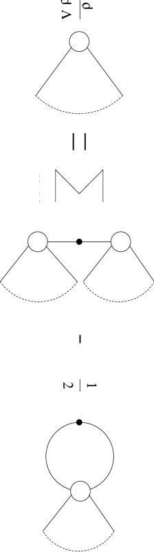
Figure 1.3: The flow equations for the vertices of the generating functional $W_{\Lambda}$. The vertices are shown as open circles. In a sharp cutoff the black dots will represent a delta function restricting momenta to $q=\Lambda$. The sum occurs over all possible disjoint partitions of momenta.

We can now transform this to an equation for $\Gamma_{\Lambda}$, the Legendre effective action, with an infra-red cutoff $\Lambda$. We define $\Gamma_{\Lambda}$, the generator of the one particle irreducible parts of the vertices, by

$$\Gamma_{\Lambda}[\phi^{c}]+\frac{1}{2}\phi^{c}_{.}C^{-1}_{.}\phi^{c}=-W_{\Lambda}[J]+J_{.}\phi^{c}$$ (1.13)

where $\phi^{c}=\frac{\delta W_{\Lambda}}{\delta J}$ is the classical field. Then using (derived in the standard way from (1.13))

$$\frac{\delta^{2}W_{\Lambda}}{\delta J\delta J}=\left(C^{-1}+\frac{\delta^{2}\Gamma_{\Lambda}}{\delta\phi^{c}\delta\phi^{c}}\right)^{-1}$$ (1.14)

we can re-write the equation as

$$\frac{\partial\Gamma_{\Lambda}[\phi^{c}]}{\partial\Lambda}=\frac{1}{2}tr\left[\frac{\partial C^{-1}}{\partial\Lambda}\;_{.}\left(C^{-1}+\frac{\delta^{2}\Gamma_{\Lambda}}{\delta\phi^{c}\delta\phi^{c}}\right)^{-1}\right]$$ (1.15)

Again all internal symmetry indices have been suppressed. This will be our starting point for all the work from now on

Note that as $\epsilon\rightarrow 0$ the $\frac{\partial C^{-1}}{\partial\Lambda}$ will restrict momentum to the shell $q=\Lambda$. Therefore, any other $C^{-1}(q)$ will contain $\theta(0)$’s, which are ambiguous [16, 26]. Extreme care must be taken with this limit.

1.4 Sharp vs. Smooth

It has come to the point where we have to decide what type of cutoff to use. In this section we will briefly describe the pros and cons of sharp [20, 32, 33] and smooth [30, 34, 35] cutoffs.

1.4.1 Sharp Cutoffs

The first problem that arises with using a sharp cutoff is how to take the sharp cutoff limit as $\varepsilon\rightarrow 0$. We mentioned above that any other term containing a $C^{-1}(q)$ becomes ambiguous in this limit. To circumvent this problem we separate the problematic terms by writing

$$\frac{\delta^{2}\Gamma_{\Lambda}}{\delta\phi\delta\phi}(p,p^{\prime})=\gamma(p,\Lambda)(2\pi)^{D}\delta(p+p^{\prime})+\hat{\Gamma}[\phi](p,p^{\prime},\Lambda)$$ (1.16)

so that $\hat{\Gamma}[0]=0$, and drop the field independent vacuum energy term. We can then write the subtracted equation as

$$\frac{\partial\Gamma_{\Lambda}}{\partial\Lambda}=-\frac{1}{2}tr\left[\frac{\partial C^{-1}}{\partial\Lambda}\;.\left(C^{-1}+\gamma\right)^{-2}.\hat{\Gamma}.\left(1+\{C^{-1}+\gamma\}.\hat{\Gamma}\right)^{-1}\right]$$ (1.17)

The sharp cutoff limit can now be taken. This is not so straightforward as it seems as we need to be able to deal with the $\theta(0)$’s that occur when we do take this limit. The answer turns out to be by no means as simple as using the usual physics convention of setting $\theta(0)=\frac{1}{2}$! To take the limit we use the following lemma:-

Let $f(\theta_{\epsilon},\Lambda)$ be any function whose dependence on the second argument remains continuous at $\Lambda=p$ in the limit $\epsilon\rightarrow 0$. Then

$$\lim_{\epsilon\rightarrow 0}\delta_{\epsilon}(p,\Lambda)f(\theta_{\epsilon}(p,\Lambda),\Lambda)\rightarrow\delta(\Lambda-p)\int^{1}_{0}dtf(t,p)$$ (1.18)

where $\delta_{\varepsilon}(p,\Lambda)=-\frac{\partial}{\partial\Lambda}\theta_{\varepsilon}(p,\Lambda)$. This is easily proved by noting that

$$\delta_{\epsilon}(p,\Lambda)f(\theta_{\epsilon}(p,\Lambda),\Lambda)=\left.\left\{\frac{\partial}{\partial\Lambda}\int^{1}_{\theta_{\epsilon}(p,\Lambda)}dtf(t,\Lambda^{\prime})\right\}\right|_{\Lambda^{\prime}=\Lambda}$$ (1.19)

and that the integral is a representation of a step function with height $\int_{0}^{1}dtf(t,\Lambda^{\prime})$. (This now yields $\delta_{\epsilon}(p,\Lambda)\theta_{\epsilon}(p,\Lambda)^{2}\rightarrow\frac{1}{3}\delta(p-\Lambda)$, which doesn’t equal the $\frac{1}{2}\delta(p-\Lambda)$ which some may have naïvely guessed.)

Using (1.18), we may now take the sharp cutoff limit in equation (1.17) to yield,

$$\frac{\partial\Gamma_{\Lambda}}{\partial\Lambda}=-\frac{1}{2}\int\frac{d^{D}q}{(2\pi)^{D}}\frac{\delta(q-\Lambda)}{\gamma(q,\Lambda)}\left[\hat{\Gamma}.\left(1+G.\hat{\Gamma}\right)^{-1}\right](\mathbf{q},\mathbf{q^{\prime}})$$ (1.20)

where we have defined,

$$\lim_{\varepsilon\rightarrow o}\frac{1}{C^{-1}(p,\Lambda)+\gamma(p,\Lambda)}=G(p,\Lambda)=\frac{\theta(p-\Lambda)}{\gamma(p,\Lambda)}$$ (1.21)

which represents a sharply infra-red cutoff, full two point Greens function.

Notice that this equation displays field re-parameterization invariance under $\hat{\Gamma}\rightarrow\lambda^{2}\hat{\Gamma},\gamma\rightarrow\lambda^{2}\gamma$ and $G\rightarrow G/\lambda^{2}$.

We now have a sharply cut-off RG equation. However, we quickly realize that any attempt to solve any of the above equations by a direct numerical approach will quickly grind to a halt due to the sheer complexity of the problem [16]. We are therefore forced to choose some approximation scheme.

As a first attempt we could try expanding in powers of field and truncating at some maximum order [36, 37, 38], ie we write (assuming a $Z_{2}$ symmetry),

$$\Gamma=\sum_{i=0}^{M}a_{i}\phi^{2i}$$ (1.22)

This expression is then substituted into equation (1.20) and the equation expanded up to a maximum power of $\phi$. This results in relationships between the coefficients which can easily be solved. This approach has been extensively investigated. However few people at first recognized certain problems with this scheme.

Firstly as pointed out in [36] the truncations at first seem to converge to an answer but stop converging after a certain value of $M$. The reason for this is that there are in fact only a finite number of true solutions [20, 39, 40], together with an infinite number of solutions with singular behaviour for some real value of $\phi$. Very bad solutions will have singular field dependence close to the origin causing the coefficients of $\phi^{2m}$ in (1.22) to diverge with m. Of course, the truncation for which the coefficient of the $2M+2$ vertex vanishes will therefore better approximate the the Taylor series of a non-singular solution. At first increasing the value of $M$ will improve the approximation, by forcing the singularities further away form the origin. However, even the non-singular solutions have singularities, but for complex $\phi$, at a radius of, say , $|\phi|=r$. Therefore the truncations can not be expected to converge to better results than would be obtained with ’moderately bad’ solutions with singular behaviour at or beyond the value of $r$. Also spurious solutions are generated and no completely reliable method can be found to reject these [36].

Taking the above into account we could try some sort of momentum expansion. It should be noted that (1.20) contains $\theta$ functions, which do not have an analytic expansion. For example,

$$\theta(|\mathbf{p}+\mathbf{q}|-1)=\theta(\mathbf{\hat{p}_{.}q}+p/2)=\theta(\mathbf{q_{.}\hat{p}})+\sum^{\infty}_{m=1}\frac{(p/2)^{m}}{m!}\delta^{(m-1)}(\mathbf{q_{.}\hat{p}})$$ (1.23)

where we have defined $\mathbf{\hat{p}}=\mathbf{p}/|\mathbf{p}|$ and $\delta^{(m-1)}$ is the $m^{\scriptsize{th}}$ derivative of the $\delta$-function with respect to its argument. The above expansion means we cannot expand in powers of $p^{2}$ but are forced to use a non-analytic expansion in powers of momentum scale, $\rho=\sqrt{p_{.}p}$, instead [16, 26].

To lowest order in the approximation we discard all external momentum dependence and write

$$\Gamma_{\Lambda}=\int d^{D}x\left\{\frac{1}{2}\left(\partial_{\mu}\phi\right)^{2}+V(\phi)\right\}$$ (1.24)

Such an ansatz yields the following equation,

$$\frac{\partial}{\partial\Lambda}V(\phi)=\ln\left(1+\frac{\partial^{2}V(\phi)}{\partial\phi\partial\phi}\right)$$ (1.25)

This forms what is known as the local potential approximation and has been extensively investigated by several authors [41, 20, 42, 32, 38]. It produces good results, although it does fail to take account of any wave function renormalization and other momentum dependent effects.

The problems arise when we try to go beyond this level of approximation. To get any further, we will eventally be forced to calculate certain averages, which appear only to be calculable, in a closed form, in certain truncations [26]. As we already know that truncations do not work we are forced to look down another avenue.

1.4.2 Smooth Cutoffs

We have rejected sharp cutoffs and we know that truncations don’t work. We also know that any attempt to use a momentum expansion (that is a derivative expansion) must preserve a re-parameterization invariance. We also know that we need to keep all powers of the fields involved as we cannot use truncations in the fields. To satisfy these requirements we will employ a derivative expansion:-

$$\Gamma[\phi]=\int d^{D}x\,V(\phi)+\frac{1}{2}\left(\partial_{\mu}\phi\right)^{2}K(\phi)+\cdots$$ (1.26)

This is substituted into (1.15) and the right hand side expanded up to a maximum number of derivatives.

The momentum expansion corresponds to a local derivative expansion in the effective Lagrangian, with radius of convergence $p\approx\varepsilon$ (this arises from the expansion of terms such $\theta_{\varepsilon}(|\mathbf{q}+\mathbf{p}|,\Lambda)$ with $q\approx\Lambda$). Since these expansions are substituted back into the flow equations and averaged over $p\approx\Lambda$ we must have $\varepsilon>\Lambda$ for convergence. Obviously the cutoff must have $\Lambda>\varepsilon$, as otherwise there would be no suppression of low momenta. Hence we see that $\varepsilon\approx\Lambda$ and typically the expansion will converge only slowly, if at all. To maximize the rate of convergence it clearly follows that we should choose the width to be as large as possible, as then we will have convergence as well as suppression of low momentum modes. We see that we are forced to use a cutoff that has a width of at least $\Lambda$ [16, 30].

To preserve a re-parameterization invariance we will use a power law additive cutoff

$$C(q,\Lambda)=\frac{q^{2k}}{\Lambda^{2k}}$$ (1.27)

for $k$ a non-negative integer. The re-parameterization invariance manifests itself in the form of a scaling symmetry with a set of (non-physical) scaling dimensions. That is if we choose

$$[q_{\mu}]=[\partial_{\mu}]=1, [\phi]=k+D/2, [\Gamma_{\Lambda}]=0,$$ (1.28)

as the non-physical scaling dimensions, then the scaling symmetry of equation (1.15) becomes apparent. We already know that we need to choose a cutoff width of at least $\Lambda$ and that convergence will be quicker the ’wider’ the cutoff function is. As we have the following identity,

$$\theta_{\varepsilon}(q,\Lambda) = \frac{q^{2}C(q,\Lambda)}{1+q^{2}C(q,\Lambda)}$$ (1.29)

$$= \frac{q^{2(k+1)}}{\Lambda^{2k}+q^{2(k+1)}}$$ (1.30)

we see that it is beneficial (ie results in the widest cutoff width) if we take $k$ as small as possible. As we also need the cutoff to regularize the theory it can be shown that $k>D/2-1$. Hence we chose $k$ to be the smallest integer greater than $D/2-1$. For $D=3$ this means we take $k=1$.

The study of the above approximation scheme will form the major part of this thesis. We will apply it to some simple problems in critical phenomena and show that it does indeed work. We leave further development of the scheme to a later chapter and we will review some of the concepts in critical phenomena required for later chapters.

1.5 Critical Phenomena

In this section we only be concerned with the problems posed by second order phase transitions. These are transitions where there is a continuous change in the properties of the system from one state to another. eg the continuous appearance of a magnetization as a ferromagnetic material is cooled. (As opposed to first order transitions where there is a discontinuous change, see [22] for details). Such phase transitions are well known, even in everyday life. For example, consider water boiling in a kettle – the liquid is changing from a liquid to a vapour. At a certain critical temperature this phase transition is second order. In fact, if we look at this transition more closely we see the phenomena known as critical opalescence, where the fluid takes on a milky appearance at the transition point. This happens exactly at the transition point and is due to regions the size of microns fluctuating coherently on a large scale. This illustrates two difficulties with critical phenomena,

• we need to consider all length scales.

• we need to consider long ranges.

This makes theoretical work extremely difficult; we find it nearly impossible to deal with problems involving just three degrees of freedom, let alone one involving maybe hundreds of thousands.

There are other problems that we would like to understand in second order transitions. For example, we would like to know why seemingly separate physical systems display very similar critical behaviour. eg uniaxial ferromagnets and fluids near their critical points display similar types of behaviour, even though they are totally different physical systems. This phenomenon is known as universality.

In the next section we describe some simple phenomenology of phase transitions and then briefly outline a theoretical background. There are many references to the subject but the books by Zinn-Justin [22] and Amit [23], and the article by Weinberg [43] are particularly good introductions.

1.5.1 Scaling

For convenience we will mostly use the language of ferromagnetic systems.

The basic quantity of interest in statistical mechanics is the free energy, $F$. This is defined by:

$$F=-kT\log Z$$ (1.31)

where Z is the partition function of the theory. For example, consider a classical spin model, so that the partition function takes the form

$$Z=\int\prod_{i}\,dS_{i}\,\rho(S_{i})\exp-\beta{\cal H}(S)$$ (1.32)

where $\beta=1/kT$, $k$ is the Boltzmann constant, $T$ is the temperature, $\rho(S_{i})$ is a spin weighting factor describing the local microscopic properties of the system, and ${\cal H}$ is the Hamiltonian given by,

$$\sum_{ij}V_{ij}S_{i}S_{j}+\sum_{i}H_{i}S_{i}$$ (1.33)

The variable $H_{i}$ in the above represents an externally applied magnetic field. Such models have achieved great success in describing simple ferromagnetic systems. The statistical average of a quantity $X$ is given by

$$<X>=\frac{1}{Z}\int\prod_{i}dS_{i}\,\rho(S_{i})X_{i}\exp-\beta{\cal H}(S)$$ (1.34)

Using this definition we define the magnetization of a system to be the average of the spins

$$M(H,T)=V^{-1}\sum_{n}a^{D}<S_{n}>$$ (1.35)

where $a$ is the lattice spacing. In what is known as the thermodynamic limit, where $N\rightarrow\infty$, we can describe the magnetization as

$$M(H,T)=-\frac{\partial}{\partial H}F(H,T)$$ (1.36)

This can easily be seen by realizing that taking a derivative with respect to $H$ brings down a $S_{i}$ into the sum. It can happen, that even in the presence of zero external magnetic field, below a certain temperature $T_{c}$ there is a non-zero value for the magnetization. When this occurs there is said to be a spontaneous magnetization and the temperature at which this first occurs is called the critical temperature.

There are other quantities of interest. The susceptibility is defined as

$$\chi(H,T)=\frac{\partial M(H,T)}{\partial H}=\frac{1}{V}\sum_{n\,m}a^{2D}<(S_{n}-<S>)(S_{m}-<S>)>$$ (1.37)

and this represents the response of a system to a small applied magnetic field. Also of interest is the specific heat which is defined as

$$C=-T\frac{\partial^{2}F}{\partial T^{2}}$$ (1.38)

Various physical quantities diverge as we approach a second order critical point. For example, the correlation function of two fluctuating fields behaves as

$$g_{nm}=<(S_{n}-<S>)(S_{m}-<S>)>\sim\exp{(-|x_{n}-x_{m}|/{\xi})}\,x^{\tau}\;\ \mbox{as $x\rightarrow\infty$ }$$ (1.39)

We call $\xi$ the correlation length. As we approach the critical temperature the correlation length diverges as follows

$$\xi\sim\begin{array}[]{cc}(T-T_{c})^{-\nu}&T>T_{c}\\ (T_{c}-T)^{-\nu^{\prime}}&T<T_{c}\end{array}$$ (1.40)

We call $\nu$ a critical exponent. Other exponents can also be defined. For example, the susceptibility diverges as

$$\chi\sim\begin{array}[]{cc}(T-T_{c})^{-\gamma}&T>T_{c}\\ (T_{c}-T)^{-\gamma^{\prime}}&T<T_{c}\end{array}$$ (1.41)

and the specific heat acts as

$$C\sim\begin{array}[]{cc}(T-T_{c})^{-\alpha}&T>T_{c}\\ (T_{c}-T)^{-\alpha^{\prime}}&T<T_{c}\end{array}$$ (1.42)

Below the critical temperature a spontaneous magnetization appears which behaves as

$$M\sim(T_{c}-T)^{\beta}$$ (1.43)

If we are exactly at the critical point, $T=T_{c}$, then the correlation function will act like

$$<(S_{n}-<S>)(S_{m}-<S>)>\sim\frac{1}{|x_{n}-x_{m}|^{D-2+\eta}}\;\ \mbox{for $a\ll|x_{n}-x_{m}|\ll\infty$}$$ (1.44)

Notice that we have lost all functional dependence on a fundamental length scale — this reflects the fact that at criticality the system is scale invariant, and is also consistent with the appearance of long range order. The exponent $\eta$ is known as the anomalous dimension.

Various relationships exist between these exponents defined at the fixed point, known as scaling relations. These mean that you only need to know two of the above critical exponents to calculate the rest. For example,

$$2\beta+\gamma = 2-\alpha$$ (1.45)

$$\gamma = \nu(2-\eta)$$ (1.46)

are the two of the best known.

These relations are easily reproduced. As an example consider the relation (1.46). To prove this, first consider the correlator of two spins (1.44). We see from equation (1.44), that when we are close to the transition point that the correlator has dimension $-D+2-\eta$. Hence, if we consider $\frac{a^{2D}}{V}\sum_{ij}g_{ij}$ then this will have scaling dimension $2-\eta$. Therefore, as the correlation length sets the basic scale of the system at criticality, so that at criticality the system loses all dependence on all other length scales, we can determine the behaviour of the magnetization, specific heat etc, in terms of the behaviour of $\xi$. This hypothesis is known as the scaling hypothesis [44]. Using the scaling hypothesis, we see that $\sum_{ij}g_{ij}$ satisfies,

$$\sum_{ij}g_{ij}\sim\xi^{2-\eta}\sim(T-T_{c})^{\nu(-2+\eta)}$$ (1.47)

near the critical point. However, a quick glance at equation (1.37) reveals that $\chi=\frac{a^{2D}}{V}\sum_{ij}g_{ij}$. Therefore, we must have

$$\chi\sim(T-T_{C})^{-\gamma}\sim(T-T_{c})^{\nu(-2+\eta)}$$ (1.48)

This then forces equation (1.46) to hold, ie $\gamma=\nu(2-\eta)$. This is known as Fisher’s scaling relation. It is also found that the indices are symmetrical about the transition point so $\alpha=\alpha^{\prime}$, $\nu=\nu^{\prime}$ etc. The reader is referred to the extensive literature on the subject for further details.

1.5.2 Critical Phenomena and the RG

In this section we will indicate how to relate the above theory to the renormalization group. We know that near criticality the correlation length is very large and we need to consider a large number of degrees of freedom. Hence, if we wish to perform calculations near the phase transition and gain a theoretical understanding of the problem, we need to find some method of reducing the number of degrees of freedom. The renormalization group does such a thing. If we continually integrate out the fluctuations with the shortest wavelength we gradually reduce the degrees of freedom, making the problem more tractable. The key point relating this to the critical point is that at criticality all wavelengths are equally important. This is because the correlation length diverges and we therefore lose all dependence on any fundamental length scale (cf equation (1.44)). This also means that as we continually integrate degrees of freedom out of the theory we essentially see the same picture — ie we are at a fixed point of the transformation.

To calculate the critical exponents we need to consider the behaviour near the fixed points. To aid this discussion we will re-write the equations in terms of dimensionless quantities. Suppose we are near a fixed point, but not on the critical surface. Equation (1.8) shows that

$$h_{i}\sim\Lambda^{-\lambda_{i}}$$ (1.49)

As the $h_{i}$’s are now dimensionless we see that we have

$$h_{i}=\left(\frac{\mu}{\Lambda}\right)^{\lambda_{i}}$$ (1.50)

Then, as the flow of the action will be dominated by the largest relevant eigenvalue, we can write,

$$\delta S_{\Lambda}\sim\left(\frac{\mu}{\Lambda}\right)^{\lambda_{L}}{\cal O}_{L}$$ (1.51)

where $\Lambda_{L}$ is the largest eigenvalue and ${\cal O}_{L}$ is the operator associated with it. We see that the integrated operator ${\cal O}_{L}$ has dimension $-\lambda_{L}$ and is associated with a coupling $\mu^{\lambda_{L}}$ of dimension $\lambda_{L}$. Now consider the situation at $\Lambda=\Lambda_{0}$. There will be an operator corresponding to the deviation from criticality. This will be the dominant operator in determining the statistical state of the system. Therefore, we associate this operator with ${\cal O}_{L}$:

$$\delta S_{\Lambda_{0}}=(T-T_{c}){\cal O}_{L}+O((T-T_{c})^{2})$$ (1.52)

As we know that the coefficient of ${\cal O}_{L}$ has dimension $\lambda_{L}$, we see that the scaling dimension of the temperature difference is also $\lambda_{L}$. Therefore, as $[\xi]=-1$, we must, have

$$\xi\sim(T-T_{c})^{-1/\lambda_{L}}$$ (1.53)

or, $\nu=1/\lambda_{L}$.

The value of $\nu$ is therefore determined by the linearization procedure. The anomalous dimension is a property of the fixed point itself — in the full un-approximated equations the value of $\eta$ is determined by the field re-parameterization invariance. The scaling symmetry of the equations turns the renormalization group equations into a non-linear eigenvalue for $\eta$, with only a few values of $\eta$ leading to acceptable fixed point solutions. By preserving the re-parameterization invariance in an approximation scheme we can still determine $\eta$ without recourse to any non-physical arguments or parameters. We can now determine two critical exponents and therefore determine the others. Corrections to the scaling behaviour are given by the subleading eigenvalues. For example, the leading correction to scaling exponent, denoted by $\omega$, is defined as being equal to minus the least negative eigenvalue. For example, close to the critical temperature we have the following scaling relation,

$$\xi\sim|T-T_{c}|^{-\nu}+\cdots$$ (1.54)

However, there are also corrections to this expression, so further away from the critical temperature we have,

$$\xi\sim|T-T_{c}|^{-\nu}+a_{\xi}|T-T_{c}|^{(\omega-1)\nu}+\cdots$$ (1.55)

1.5.3 Critical Phenomena and Field Theory

We have now reached the stage where we should relate physical systems to field theoretical models. It should have been realized by now that there are two equivalent descriptions of critical phenomena. In the above we have sometimes used the language of classical spin like systems and sometimes we have found it more convenient to use a field-theoretical like language. There is in fact an intrinsic link between the two descriptions and we will make an attempt to briefly describe the relation between the descriptions. Consider the classical spin model defined above by equation (1.33). If we assume that the lattice is hyper-cubic and that we only have nearest neighbour couplings then we can write

$$\sum_{ij}V_{ij}S_{i}S_{j}=K\sum_{n}\left(\sum_{\mu}(S_{n+\mu}-S_{n})^{2}-2dS_{n}^{2}\right)$$ (1.56)

where $\mu$ runs over the directions of the lattice. In fact, if we consider a model where the spin is constrained by $S^{2}=\pm 1$ (known as the Ising model), we can describe this using a spin weighting function of (taking an appropriate choice of $\lambda$ and $\kappa$),

$$\rho(S_{i})\propto\exp-(\kappa S_{n}^{2}+\lambda S_{n}^{4})$$ (1.57)

We can then write the Hamiltonian as

$${\cal H}=\sum_{n}\left(K(\beta)\sum_{\mu}(S_{n+\mu}-S_{n})^{2}+\mu(\beta)S_{n}^{2}+\lambda(\beta)S_{n}^{4}+H_{n}S_{n}\right)$$ (1.58)

[It is perhaps worth pointing out that other versions of the spin-weighting function (1.57), with terms of higher powers in $\phi$ could also be used. However it turns out that such terms are irrelevant, in the sense defined above, and have no influence on the critical theory.]

The above expression (1.58) for the Ising Hamiltonian should look familiar — it looks like a lattice regularized $\phi^{4}$ theory [45]. To see this take a massive $\phi^{4}$ in $D$ dimensions,

$$S(J)=\int d^{D}x\left(\frac{1}{2}(\partial_{\mu}\phi)^{2}+\frac{1}{2}m^{2}\phi^{2}+\frac{\lambda}{4!}\phi^{4}\right)$$ (1.59)

and place it on a hyper-cubic lattice by writing,

$$x \mapsto x_{n}=an_{\mu}\hat{e}_{\mu}$$ (1.60)

$$\phi(x) \mapsto \phi_{n}=\phi(x_{n})$$ (1.61)

$$D\phi \mapsto \prod_{n}d\phi_{n}$$ (1.62)

$$\partial_{\mu}\phi \mapsto \frac{1}{a}\left(\phi(x_{n}+\hat{e}_{\mu})-\phi(x_{n})\right)=\frac{1}{a}(\phi_{n+\mu}-\phi_{n})$$ (1.63)

where $a$ is the lattice spacing and $\hat{e}_{\mu}$ is a set of $D$ orthonormal vectors. Under these transformations the lattice regularized theory is

$$S(\phi,J)=\sum_{n}a^{D}\left\{\frac{1}{a^{2}}\sum_{\mu}\frac{1}{2}\left(\phi_{n+\mu}-\phi_{n}\right)^{2}+m^{2}\phi_{n}^{2}+\lambda\phi_{n}^{4}+J_{n}\phi_{n}\right\}$$ (1.64)

and the partition function becomes,

$$Z(J)=\prod_{n}\int d\phi_{n}\exp S(\phi,J)$$ (1.65)

where the functional measure $D\phi$ is replaced by a finite dimensional integral $\prod_{n}d\phi_{n}$.

The correspondence between (1.59) and (1.58) should now be clear. So we see that there is a direct link between lattice theories and the Ising model. However, what we are really interested in is the critical theory. To clearly see the link we will have to show explicitly what happens at the phase transition and consider the ground states of the Ising model.

Consider the potential of the model $\mu(\beta)S^{2}+\lambda(\beta)S^{4}$, where for the moment we will ignore quantum corrections (ie we will use what is known as mean field theory [22]). For $\mu(\beta)>0$ we have a potential like figure (1.4a). We see we have a ground state in which $S_{n}=0$ and

$$<S>=\frac{1}{V}\sum_{n}S_{n}=0\ \ \mbox{ for $\mu({\beta})>0$}$$ (1.66)

If $\mu(\beta)<0$ then we have a potential like figure (1.4b). Now the ground state corresponds to the $S_{n}$ aligned with $S_{n}=\sqrt{\frac{-\mu}{2\lambda}}$, so that

$$<S>=\sqrt{\frac{-\mu}{2\lambda}}\ \ \mbox{ for $\mu({\beta})<0$}$$ (1.67)

We see that the phase transition corresponds to the point where $\mu=0$. The temperature that corresponds to this is called the critical temperature.

(a) $\mu>0$

(b) $\mu<0$

Figure 1.4: The potential, $\mu(\beta)S^{2}+\lambda(\beta)S^{4}$, for the unbroken case $\mu>0$ (a), and the broken case $\mu<0$, (b).

Now let us make the correspondence between the critical Ising model and and the critical lattice theory. To make direct comparisons we first move to non-dimensional variables. That is we write

$$\lambda=g^{2}a^{D-4}, \phi^{\prime}=ga^{\frac{D}{2}-1}\phi, \mbox{and}\ \ J^{\prime}=ga^{D/2+1}J$$ (1.68)

the action then becomes

$$S(\phi^{\prime},J^{\prime})=-\frac{1}{g^{2}}\sum_{n}\left\{\frac{1}{2}\sum_{\mu}(\phi^{\prime}_{n+\mu}-\phi^{\prime}_{n})^{2}+\frac{1}{2}m^{2}a^{2}\phi^{\prime 2}_{n}+\frac{1}{4!}\phi^{\prime 4}_{n}+J^{\prime}\phi^{\prime}_{n}\right\}$$ (1.69)

We see comparing equations (1.58) and (1.69) that we have the following correspondence,

$$m^{2}a^{2}\sim\mu(\beta)$$ (1.70)

We know that as we approach the critical temperature $\mu(\beta)\rightarrow 0$. This forces us to fine tune $a$ to zero as well, as the physical mass of the system $m$ must be held fixed. Hence, we see that as we approach the fixed point we must also approach the continuum limit.

We should really have expected this on heuristic arguments:- we know that at the critical point the Ising model is scale invariant. Therefore to preserve this invariance we cannot have any massive parameter in the field theoretical model and so there cannot be any cutoff involved. We can also use this argument to show that the critical theory corresponds to a massless theory — any mass involvement in the critical theory would break scale invariance. We see that the critical theories correspond to massless, renormalized theories.

We now have a definite link between field theories and the statistical mechanics of critical phenomena. There is one final missing link in our puzzle — how to relate the theory to physical systems. This is not as complex as may first be thought. For most simple systems it is possible to find local observables whose values depend upon the phase that they are in. For example, in the above the spin played the role of the order parameter, differentiating between the phase with a spontaneous magnetization and the one without. The relation of a physical theory and a theoretical analysis boils down to determining what are the order parameters and what are their internal symmetries. For example, the order parameter for the helium superfluid transition is complex having a continuous symmetry corresponding to multiplication by a phase. This can be shown to be equivalent to a theory of two real scalar fields. Therefore, we may use a field theory consisting of a real scalar field with a global $O(2)$ symmetry.

We will primarily concentrate on systems described by $O(N)$ symmetric scalar field theories with the following action

$$S=\int d^{D}x\left\{\frac{1}{2}\left(\partial_{\mu}\mathbf{\Phi^{a}(x)}\right)^{2}+\frac{m^{2}}{2}\mathbf{\Phi^{a}(x)\Phi^{a}(x)}+\frac{g}{4!}\left({\mathbf{\Phi^{a}(x)\Phi^{a}(x)}}\right)^{2}\right\}$$ (1.71)

As usual the index a refers to an internal symmetry under the $O(N)$ group. These models correspond to different physical systems according to the value of $N$ (see [22] for details on how to derive these),

N=0

critical behaviour of polymers. This is only formally defined in the limit $N\rightarrow 0$, as first noted by de Gennes [46].

N=1

the liquid-vapour phase transition [47], the alloy order-disorder transition, uniaxial ferromagnets. We see that here we have no internal symmetries involved. eg the liquid-vapour transition can be modelled by particles living on a lattice: allowing the occupation of each lattice site to be either be 0 or 1 leads to a link with the Ising model [48].

N=2

$\mathit{He}^{2}$ superfluid phase transition, planar ferromagnets. The first example was discussed above. The planar ferro-magnet will clearly have a symmetry in a plane. This then leads to the choice of a two component field with an $O(2)$ symmetry between the two components.

N=3

ferro magnetic phase transitions. Now we have a true three dimensional symmetry so a three field order parameter is chosen, with an $O(3)$ symmetry between the components.

N=4

It has been postulated that this corresponds to the chiral phase transition for two flavours of quarks [49].

The fact that one model for a particular value of $N$ can descibe several physical systems is the theoretical basis of universality. It should also be noted that it doesn’t matter what the initial value of any coupling is, or the lattice spacing or even upon the shape of the lattice: once we have adjusted the temperature (or pressure, density etc,..) so that we are on the critical surface, we know that renormalization group transformations will take us into a fixed point, which will yield the same critical behaviour. In fact we can take this further and ask why do different materials have the same critical behaviour. eg in critical binary fluids, which correspond to $N=1$, $D=3$, a mixture of aniline and cyclohexane shows the same critical behaviour as a mixture of triethlamine and water [50]. This is because the critical behaviour is independent of the underlying structure of the physical system. At distances of order of the lattice spacing the detailed fine structure, such as the lattice spacing and the lattice structure, will be important. However when we use the renormalization group to decrease the amount of ’magnification’ these details are washed out, as the details at the scale of the lattice will be averaged out [51].

1.5.4 Other methods of investigating critical behaviour.

Before going any further we briefly consider other methods of investigating critical phenomena and calculating exponents.

Original predictions of critical exponents were made using mean field theory in which a saddle point expansion is made about the classical minimum of the field equations. Exact predictions for the exponents are made. In fact for the $O(N)$ models descibed above the predictions are independent of the value of $N$. The main problems occur when we try to go beyond the tree level expansion. Below four dimensions infra-red divergences plague an expansion making it useless [22, 23].

To go beyond mean field theory Wilson and Fisher developed what is known as the $\varepsilon$ expansion. The dimension of space is taken as $4-\varepsilon$ and a double expansion is made in the coupling constant $g$ of the theory and $\varepsilon$. Thus, for example, a $n$-point function may be expanded as

$$\Gamma^{n}(p_{1},\ldots,p_{n})=\sum_{rs}\Gamma_{rs}^{(n)}g^{r}\varepsilon^{s}$$ (1.72)

This coupled with a renormalization group analysis has produced some spectacular results. This method avoids the infra-red divergences by moving from a gaussian fixed point to the non-trivial, infra-red stable Wilson-Fisher fixed point [22]. The $\varepsilon$ expansion has enjoyed considerable success and has made accurate predictions of the exponents. However it does have some drawbacks. For example the series it produces is only asymptotic and requires Borel resummation [22].

The $N$ vector model has also been studied on lattices with nearest neighbour interactions. The results for the exponents come from analysis using high temperature series by different types of ratio method, Padé approximants or differential approximants. For large $N$, the $1/N$ expansion has also been used. However the large $N$ models are unphysical and are only studied out of theoretical interest (the main one being that the $N=\infty$ model is exactly solvable).

There are various other methods that have been used to calculate critical exponents which deserve a mention. The real space renormalization group method [52] consists of considering spins on a lattice and performing blocking transformations to reduce the number of degrees of freedom, and then truncating the resulting expression at a certain number of operators. Similar in style are Monte-Carlo renormalization group calculations [53, 54, 55]. Here the path integral is expanded in a certain set of operators and a blocking transformation performed. A Monte-Carlo calculation is then performed to calculate what values the couplings associated with these operators should have afterwards. Finally there is perturbation in fixed dimension [22]. Developed by Parisi, this consists of calculating the $\beta$ function in perturbation theory at a fixed dimension. The resulting expression can then be re-summed to provide information about the zero’s of the $\beta$ function and hence information about the critical exponents.

Chapter 2 The Results at Leading Order

In the introduction we outlined why an approximation scheme based upon a derivative expansion of the renormalization group equations is sensible approach to analytic non-perturbative calculations. In this chapter we will report the results of applying the derivative expansion at the leading order in the approximation to a theory with a global $O(N)$ symmetry, and calculate the critical exponents $\eta$, $\nu$ and $\omega$.

2.1 Deriving the Leading Order Equation

Our starting point will be the flow equation for the Legendre effective action,

$$\frac{\partial\Gamma_{\Lambda}[\phi]}{\partial\Lambda}=\frac{1}{2}tr\left[\frac{\partial C^{-1}}{\partial\Lambda}\;_{.}\left(C^{-1}\delta^{ab}+\frac{\delta^{2}\Gamma_{\Lambda}}{\delta\phi^{a}\delta\phi^{b}}\right)^{-1}\right]$$ (2.1)

where we have dropped the superscript $c$ on the $\phi$’s, denoting the classical field, and re-introduced the internal symmetry indices. The trace represents a sum over the internal spin indices and an integration over momentum/position space. As in [16] it is convenient to write the trace as an integral over momentum space and factor out the $D$-dimensional solid angle:

$$\frac{\partial\Gamma_{\Lambda}[\phi]}{\partial\Lambda}=-\frac{\Omega}{2}\mathrm{tr}\int^{\infty}_{0}dq\,\frac{q^{D-1}}{C(q,\Lambda)}\frac{\partial C(q,\Lambda)}{\partial\Lambda}\left\langle\left[\delta^{ab}+C.\frac{\delta^{2}\Gamma_{\Lambda}}{\delta\phi^{a}\delta\phi^{b}}\right]^{-1}(\mathbf{q},\mathbf{-q})\right\rangle$$ (2.2)

where $\Omega=2/[\Gamma(D/2)(4\pi)^{D/2}]$ is the solid angle of a $D-1$-dimensional sphere divided by $(2\pi)^{D}$, the brackets $\langle\cdots\rangle$ represent an average over all directions of the momentum $\mathbf{q}$, and the trace now represents only the trace over the spin indices, $a$ and $b$.

It is not yet clear how the anomalous dimension will be determined. At a fixed point we know the field $\phi$ scales anomalously as $\phi\sim\Lambda^{D_{\phi}}$, where $D_{\phi}=\frac{1}{2}(D-2+\eta)$ and $\eta$ is the anomalous scaling dimension. Considering the defining expression for $\Gamma_{\Lambda}$, $\Gamma_{\Lambda}[\phi]=-\frac{1}{2}\phi.C^{-1}.\phi-W_{\Lambda}[J]+J_{.}\phi$, dimensional analysis then shows that we require $C$ to behave as follows,

$$C(q,\Lambda)\rightarrow\Lambda^{\eta-2}\tilde{C}(q^{2}/\Lambda^{2})$$ (2.3)

for some $\tilde{C}$, if we are to have $\Gamma_{\Lambda}$ independent of $\Lambda$ as we approach the fixed point. From now on we will write $C(q,\Lambda)$ as $\Lambda^{\eta-2}\tilde{C}(q^{2}/\Lambda^{2})$ and drop the tilde on the scaled $C$. As we are only interested in the behaviour near or at fixed points this is a sensible definition and we can take $\eta$ to be a constant. This is another reason for choosing an additive cutoff. A multiplicative cutoff would not scale anomalously, as is required if we wish to reach non-Gaussian fixed points [30]. From this discussion we see that it will be particularly convenient to re-write the equations in terms of dimensionless variables,

$$\mathbf{q} \rightarrow \Lambda\mathbf{q}$$

$$\phi(\Lambda\mathbf{q}) \rightarrow \Lambda^{D-D_{\phi}}\phi(\mathbf{q})$$ (2.4)

We will also re-write the equations in terms of $t=\log(\Lambda_{0}/\Lambda)$ and rescale the fields and the effective action to absorb the factor of $\Omega/2$ in (2.2),

$$\Gamma \rightarrow \frac{\Omega}{2\zeta}\Gamma$$

$$\phi^{a} \rightarrow \sqrt{\frac{\Omega}{2\zeta}}\phi^{a}$$

where we have dropped the subscript on $\Gamma$, and $\zeta$ is a normalization factor to be chosen for later convenience. Upon doing this we get,

$$(\frac{\partial}{\partial t}+D_{\phi}\Delta_{\phi}+\Delta_{\partial}-D)\Gamma[\phi]=$$

$$-\zeta\,\mathrm{tr}\int^{\infty}_{0}dq\,q^{D-1}\left(\frac{q}{C(q^{2})}\frac{\partial C(q^{2})}{\partial q}+2-\eta\right)\left\langle\left[\delta^{ab}+C_{.}\frac{\delta^{2}\Gamma}{\delta\phi^{a}\delta\phi^{b}}\right]^{-1}(\mathbf{q},-\mathbf{q})\right\rangle$$

In the above $\Delta_{\phi}=\phi.\frac{\delta}{\delta\phi}$ is the field counting operator: it counts the number of occurrences of the field $\phi$ in a given vertex, and arises due to the scaling of the field in (2.4). $\Delta_{\partial}$ is the momentum counting operator plus the dimension of space $D$ and arises through the rescaling of the momenta in equation (2.4). It can be represented as

$$\Delta_{\partial}=D+\int\frac{d^{D}p}{(2\pi)^{D}}\phi(\mathbf{p})p^{\mu}\frac{\partial}{\partial p^{\mu}}\frac{\delta}{\delta\phi(\mathbf{p})}$$ (2.6)

Operating on a given vertex it counts the total number of derivatives acting on the fields $\phi$.

Equation (2.1) will be the starting point for all the work from now onwards. Notice that for the first time $\eta$ explicitly appears in the equation.

We write $\Gamma[\phi]$ as the space-time integral of an effective Lagrangian expanded in powers of derivatives,

$$\Gamma[\phi]=\int d^{D}x\left\{V(\phi^{2},t)+\frac{1}{2}K(\phi^{2},t)\left(\partial_{\mu}\phi^{a}\right)^{2}+\frac{1}{2}Z(\phi^{2},t)\left(\phi^{a}\partial_{\mu}\phi^{a}\right)^{2}+\cdots\right\}$$ (2.7)

Each linearly independent (under integration by parts) combination of differentiated fields will carry its own general (t-dependent) coefficient. The global $O(N)$ symmetry forces us to choose the coefficient functions to be functions of $\phi^{2}$. We will require that the fixed point solutions for $V$,$K$,$Z$ etc will be non-singular for all $\phi^{2}$, that perturbations about these solutions grow no faster than a power, and that $K(0)\neq 0$.

The rescaling symmetry is made explicit by choosing the following (non-physical) scaling dimensions, as follows from (2.7) and the definition of $\Gamma$.

$$[q^{\mu}]=1 [\partial^{\mu}]=1 [\phi^{a}]=k+D/2$$ (2.8)

$$\mbox{}[V]=D [K]=-2(k+1) [Z]=-2(2k+2)-D$$

where $k$ is the exponent in the cutoff function, $C(q^{2})=q^{2k}$. The expansion is performed by substituting equation (2.7) into equation (2.1) and expanding the right hand side up to a maximum number of derivatives (in this chapter this will be no derivatives). The angular average in (2.1) can be easily computed by translating them into invariant tensors, eg $\langle q^{\mu}q^{\nu}\rangle=q^{2}\delta^{\mu\nu}/D$ etc. From now on we will specialize to $D=3$.

To lowest order in the expansion we drop all the derivatives from the right hand side of (2.1). The coefficient functions $K$,$Z$, etc are then determined by linear equations given by the vanishing of the left hand side of (2.1). Consider the equations for $K$,

$$\frac{\partial}{\partial t}K(\phi^{2},t)+(1+\eta)\phi^{2}K^{\prime}(\phi^{2},t)+\eta K(\phi^{2},t)=0$$ (2.9)

We see that at fixed points, where $\partial/\partial t=0$, this then predicts

$$K(\phi^{2})\propto(\phi^{2})^{-\eta/(1+\eta)}$$ (2.10)

where ${}^{\prime}=\frac{\delta}{\delta\phi^{2}}$. To avoid $K(\phi^{2})$ being singular and ensure that $K(0)\neq 0$ we see we must have $\eta=0$. Therefore $K(\phi^{2})$ must be a constant. Using the scaling symmetry we can set this constant to be $1$.

If we now consider the equation for $Z$ we get

$$\frac{\partial}{\partial t}Z(\phi^{2},t)+\phi^{2}Z^{\prime}(\phi^{2},t)+Z(\phi^{2},t)=0$$ (2.11)

Hence, we see that at fixed points that $Z$ will satisfy,

$$Z\propto(\phi^{2})^{-1}$$ (2.12)

Again to avoid non-singular behaviour we set the constant of proportionality to zero and get $Z(\phi^{2})\equiv 0$. In general, considering the form of a general term in the expansion we see that a similar conclusion must hold for all other terms. A general term, $H$, will satisfy

$$\frac{\partial}{\partial t}H(\phi^{2},t)+(\phi^{2}H^{\prime}(\phi^{2},t)+n_{\phi}H(\phi^{2},t))+n_{\partial}H(\phi^{2},t)-3H(\phi^{2},t)=0$$ (2.13)

where $n_{\phi}$ is the number of $\phi$’s occurring in the term multiplying $H$, divided by two, and $n_{\partial}$ is the number of derivatives occurring in the term multiplying $H$. Hence we see that at a fixed point, where $\eta$ must be zero, we have

$$H\propto(\phi^{2})^{-(n_{\phi}+n_{\partial}-3)}$$ (2.14)

We see that for terms of higher order in the expansion, where $n_{\phi}>2$ and $n_{\partial}>2$, that $H$ will be singular unless the constant of proportionality is set to zero. Therefore, at leading order, the derivative expansion must reproduce the local potential expansion at fixed points:

$$\Gamma[\phi]=\int d^{D}x\,V(\phi^{2})+\frac{1}{2}(\partial_{\mu}\phi^{a})^{2}$$ (2.15)

The next step is to calculate the trace of the following expression,

$$\left[\delta^{ab}+C.\frac{\delta^{2}\Gamma[\phi]}{\delta\phi^{a}\delta\phi^{b}}\right]^{-1}(\mathbf{q},\mathbf{-q})=\left[\delta^{ab}+2q^{2}\left\{\delta^{ab}V^{\prime}+2\phi^{a}\phi^{b}V^{\prime\prime}+q^{2}\delta^{ab}\right\}\right]^{-1}$$ (2.16)

Working in momentum space and integrating by parts where necessary we have,

$$\frac{\delta^{2}\Gamma[\phi]}{\delta\phi^{a}\delta\phi^{b}}=2\delta^{ab}V^{\prime}+4\phi^{a}\phi^{b}V^{\prime\prime}+q^{2}\delta^{ab}$$ (2.17)

The taking of the trace over the spin indices of (2.16) is easily accomplished by noting that an operator $A\delta^{ab}+B\phi^{a}\phi^{b}$ has eigenvalues $A$ and $A+\phi^{2}B$, with the eigenvalue $A$ having multiplicity $N-1$, where $N$ is the dimension of the internal symmetry space. Hence, provided that $A\neq 0$ and $A+\phi^{2}B\neq 0$, then $[A\delta^{ab}+B\phi^{a}\phi^{b}]^{-1}$ has eigenvalues $1/A$, with multiplicity $N-1$, and $1/(A+\phi^{2}B)$. Hence we must have $\mathrm{tr}[A\delta^{ab}+B\phi^{a}\phi^{b}]^{-1}=(N-1)/A+1/(A+B\phi^{2}$). Therefore, taking the trace of equation (2.16) gives

$$\frac{N-1}{1+2V^{\prime}q^{2}+q^{4}}+\frac{1}{1+(2V^{\prime}+4\phi^{2}V^{\prime\prime})q^{2}+q^{4}}$$ (2.18)

The leading order equation has now become

$$\frac{\partial V(\phi^{2},t)}{\partial t}+\phi^{2}V^{\prime}(\phi^{2},t)-3V(\phi^{2},t)=$$

$$-4\zeta\int dq\,q^{2}\frac{N-1}{1+2V^{\prime}(\phi^{2},t)q^{2}+q^{4}}+\frac{1}{1+(2V^{\prime}(\phi^{2},t)+4\phi^{2}V^{\prime\prime}(\phi^{2},t))q^{2}+q^{4}}$$

Performing the $q$-integrals, doing the trivial angular average and setting $\zeta$ to $1/2\pi$ yields the equation at leading order,

$$\frac{\partial V(\phi^{2},t)}{\partial t}+\phi^{2}V^{\prime}(\phi^{2},t)-3V(\phi^{2},t) = -\frac{1}{\sqrt{2+2V^{\prime}(\phi^{2},t)+4\phi^{2}V^{\prime\prime}(\phi^{2},t)}}$$ (2.20)

$$-\frac{N-1}{\sqrt{2+2V^{\prime}(\phi^{2},t)}}$$

In the rest of this chapter we will report the results of the study of this equation.

2.2 Fixed Point Solutions

We are now ready to start the search for fixed point solutions of (2.20), that is solutions with $\partial/\partial t=0$. At first sight it may seem that (2.20) has infinitely many solutions parameterized by the value of $V^{\prime\prime}(0)$. In fact this is not the case, as only finitely many solutions do not end in a singularity [40, 20]. Of course this is sensible on physical grounds, as the fixed points correspond to massless continuum limits (ie second order phase transitions) with the prescribed field content. To see that we should only expect to see a discrete set of solutions we must consider the boundary conditions supplied to (2.20).

The only requirement we have imposed upon $V(\phi^{2})$ so far is that it is non-singular for all $\phi^{2}$. Considering the form of (2.20), we see that this implies that either $V(\phi^{2})$ is trivial (the Gaussian fixed point), or that $V(\phi^{2})$ must satisfy the following for large $\phi^{2}$,

$$A_{v}\;(\phi^{2})^{3}+\frac{\sqrt{30}}{120}\frac{(\sqrt{5}(N-1)+1)}{\phi^{2}\sqrt{A_{v}}}+O((\phi^{2})^{-2})$$ (2.21)

for some constant $A_{v}$.

If we consider the perturbations about this solution we see that at large $\phi^{2}$ the perturbation must behave as a combination of $\exp(\frac{1}{8}[30A_{v}]^{3/2}(\phi^{2})^{3/2})$ and $(\phi^{2})^{3}$. The second perturbation merely alters the value of $A_{v}$, whilst we disallow the first as it is incompatible with (2.21). We see that the solution space of fixed point solutions, defined for all $\phi^{2}$ and satisfying (2.21), divides up into an isolated one parameter set, parameterized by the value of $A_{v}$.

The only other possibility that makes the two sides of (2.20) balance is that $V(\phi^{2})$ is only defined for $\phi^{2}<\phi_{c}^{2}$ and ends at a singularity, at $\phi^{2}=\phi_{c}^{2}$ as follows,

$$\frac{1}{\phi_{c}^{2}}\left(\frac{27}{16}\right)^{2/3}\left(\phi_{c}^{2}-\phi^{2}\right)^{4/3}$$ (2.22)

where we have suppressed non-singular and lower order-singular parts. Notice that if either $V$ or $V^{\prime}$ where to diverge then it would not be possible for both sides of equation (2.20) to balance. We will disregard these non-physical singular solutions.

The imposition of the $O(N)$ symmetry forces $V$ to be a function of $\phi^{2}$, so it is symmetric under the $Z_{2}$ transformation $\phi^{a}\leftrightarrow-\phi^{a}$. To ensure this, we need $V(\phi^{2})$ to exist at the origin and satisfy (2.20) there. Setting $\phi^{2}=0$ in equation (2.20) gives us our final boundary condition,

$$-3V(0)=-\frac{N}{\sqrt{2+2V^{\prime}(0)}}$$ (2.23)

We now have a second order differential equation with two boundary conditions. Thus we expect at most a discrete set of acceptable solutions. In fact we only find two:- the Gaussian fixed point and an approximation to the Wilson-Fisher fixed point [14].

2.2.1 The Gaussian Fixed Point

It can be quickly seen that imposing $V^{\prime}(\phi^{2})=0$ and $V^{\prime\prime}(\phi^{2})=0$ that a trivial fixed point solution exists,

$$V(\phi^{2})=\frac{N}{3\sqrt{2}}$$ (2.24)

This is the fixed point mentioned in the introduction.

2.2.2 The Wilson-Fisher Fixed Point

A more interesting case is when the solution is non-trivial. We only find one example of a non-trivial point, which we deem to be an approximation to the Wilson-Fisher fixed point. To find this fixed point we need to rely on numerical methods as outlined in appendix A. We will impose (2.23) as a condition at the origin and force non-trivial behaviour by imposing (2.21) as $\phi^{2}\rightarrow\infty$. The results of these calculations are shown in figure (2.1) for various values of $N$.

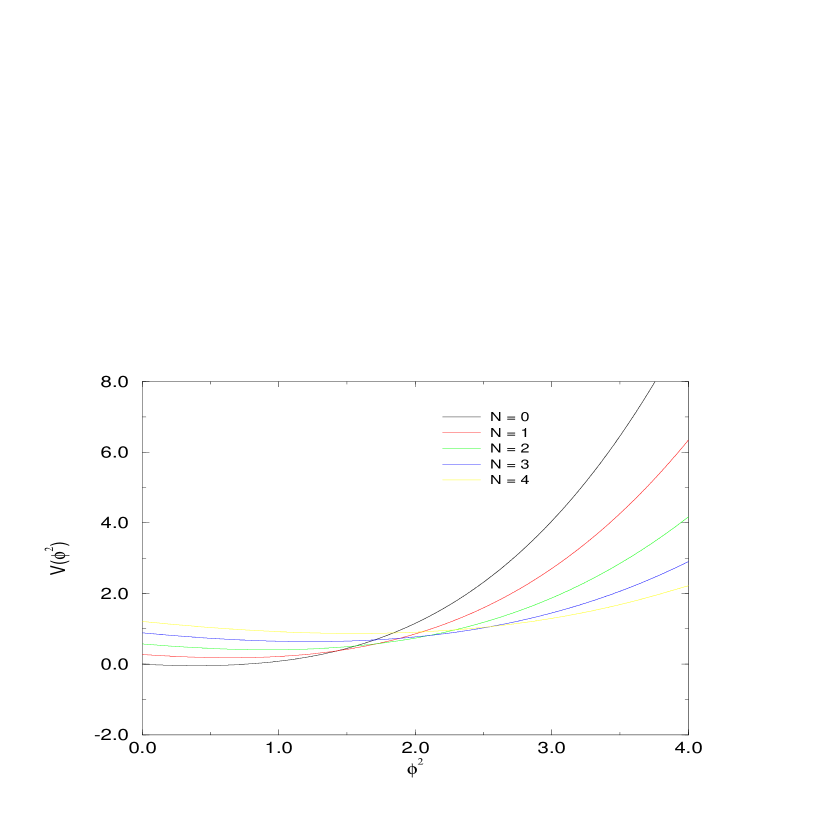
Figure 2.1: The potential at leading order in the derivative expansion for $D=3$, $O(N)$ symmetric field theory, for $N=0,1,2,3,4$.

2.3 Critical Exponents at Leading Order

The next step in the program is to calculate the critical exponents for $\nu$ and $\omega$ corresponding to the fixed points. To calculate the critical exponents it is necessary to linearize about this fixed point potential, $V^{*}(\phi^{2})$. We will write $V(\phi^{2},t)=V^{*}(\phi^{2})+\delta V(\phi^{2})$, where $\delta V(\phi^{2},t)$ is given by $\varepsilon\mathrm{e}^{\lambda t}v(\phi^{2})$, with $\varepsilon\ll 1$, and expand to first order in $\varepsilon$. Upon doing this we have

$$(\lambda-3)v(\phi^{2})+v^{\prime}(\phi^{2})\phi^{2}=\frac{N-1}{(2+2V^{\prime}(\phi^{2}))^{3/2}}v^{\prime}(\phi^{2})+\frac{v^{\prime}(\phi^{2})+2\phi^{2}v^{\prime\prime}(\phi^{2})}{(2+2V^{\prime}(\phi^{2})+4\phi^{2}V^{\prime\prime}(\phi^{2}))^{3/2}}$$ (2.25)

2.3.1 Critical Exponents for the Gaussian Fixed Point

For the Gaussian fixed point we will expect to find perturbations with eigenvalues given by the classical scaling dimension of the coupling (cf Introduction), eg an operator corresponding to the mass with dimension 2, an operator corresponding to the $\phi^{4}$ interaction with dimension $1$ etc. In the case of the Gaussian fixed point equation (2.25) becomes,

$$(\lambda-3)v(\phi^{2})+v^{\prime}(\phi^{2})\phi^{2}=\frac{Nv^{\prime}(\phi^{2})}{2\sqrt{2}}+\frac{2\phi^{2}v^{\prime\prime}(\phi^{2})}{2\sqrt{2}}$$ (2.26)

The general solution to this equation is

$$A_{[\lambda-3]}F(\sqrt{2}\phi^{2})_{[N/2]}+B2^{-\lambda/2+3/2}(\phi^{2})^{3-\lambda}_{[\lambda-3,-2+\lambda-N/2]}F(-\frac{1}{\sqrt{2}\phi^{2}})_{[]}$$ (2.27)

where ${}_{[a_{1},a_{2},\ldots,a_{i}]}F(x)_{[b_{1},b_{2},\ldots,b_{j}]}$ represents Barnes’ extended hypergeometric function,defined by,

$${}_{[a_{1},\ldots,a_{i}]}F(x)_{[b_{1},\ldots,b_{j}]}=\sum_{k=0}^{\infty}\frac{\left(\prod_{m=1}^{i}\frac{\Gamma(a_{m}+k)}{\Gamma(a_{m})}\right)}{\left(\prod_{n=1}^{j}\frac{\Gamma(b_{n}+k)}{\Gamma(b_{n})}\right)}x^{k}$$ (2.28)

If any of the $a_{i}=-k$, for $k$ a non-positive integer, then the series stops after $k$ terms. If we wish the solutions to be bounded by polynomials then we are forced to set the coefficient $B$ in the above to zero and chose $\lambda-3=k$, for some negative integer $k$. This then forces $\lambda=2,1,0,-1,\ldots$, and we have the expected results. We see that the at the Gaussian fixed point the scaling dimensions are given by the canonical dimensions [20], that $\eta=0$ and $\nu=1/2$.

2.3.2 Critical Exponents at the Wilson-Fisher Fixed Point

To calculate the exponents at the non-trivial fixed point we will need to think about the boundary conditions. By linearity of the perturbation we can choose $v(0)=1$. We will again ensure that the perturbation exists at the origin by imposing the equation as a boundary condition at $\phi^{2}=0$. That is,

$$(\lambda-3)v(0)=\frac{N}{(2+2V^{\prime}(0))^{3/2}}v^{\prime}(0)$$ (2.29)

The case $N=0$ is treated slightly differently. If we were to impose (2.29) then we either have $\lambda=3$ or $v(0)=0$. We discard the case of $\lambda=3$ as this corresponds to the uninteresting case of the vacuum energy operator. We must therefore have $v(0)=0$. The other boundary condition again comes from linearity, which we take to be $v^{\prime}(0)=1$.

We can also consider the solutions for large $\phi^{2}$. This time we will see that the perturbation will be a linear combination of $(\phi^{2})^{3-\lambda}$ and $\exp(\frac{1}{8}[30Av]^{3/2}(\phi^{2})^{3/2})$. Once more we will enforce a coefficient of zero on the latter perturbation, as we require the perturbations to grow no faster than a power in $\phi^{2}$. The imposition of this condition will ensure that the solutions satisfying $(\phi^{2})^{3-\lambda}$ as $\phi\rightarrow\infty$ form an isolated one parameter set.

Upon imposing these two conditions we will have a second order eigenvalue problem for $\lambda$ with three boundary conditions. Therefore, we expect to see a discrete number of solutions, which is indeed the case. We find only one positive eigenvalue, which yields $\nu$ through $\nu=1/\lambda$. The least negative eigenvalue yields the first correction to scaling through $\omega=-\lambda$. The results are summarized in table (2.1).

$N$	$\nu$		$\omega$
		$0.5880^{a}$		$0.80(4)^{a}$
0	$0.5961$	$0.5880(15)^{b}$	$0.6175$	$0.82(4)^{b}$
		$0.592(3)^{c}$
		$0.6300(15)^{a}$		$0.79(3)^{a}$
1	$0.6604$	$0.6310(15)^{b}$	$0.6285$	$0.81(4)^{b}$
		$0.6305(15)^{c}$
		$0.6695(20)^{a}$		$0.78(25)^{a}$
2	$0.7253$	$0.671(5)^{b}$	$0.6621$	$0.80(4)^{a}$
		$0.672(7)^{c}$
		$0.705(3)^{a}$		$0.78(2)^{a}$
3	$0.7811$	$0.710(7)^{b}$	0.7068	$0.79(4)^{b}$
		$0.715(20)^{c}$
4	$0.8240$	$0.7479(90)^{e}$	$0.7510$
10	$0.9380$	$0.877^{d}$	$0.8910$	$0.78^{f}$
20	$0.9577$	$0.942^{d}$	$0.9469$	$0.89^{f}$
100	$0.9938$	$0.989^{d}$	$0.9911$	$0.98^{f}$

Table 2.1: Critical exponents of the three-dimensional theory for various values of $N$. For comparison we list results obtained with other methods:
a) From summed perturbation series in fixed dimension 3 at six-loop order [22].
b) From the $\varepsilon$-expansion at order $\varepsilon^{5}$ [22].
c) From lattice calculations [22].
d) From the $1/N$-expansion at order $1/N^{2}$ [56].
e) From a recent lattice study [57].
f) From the $1/N$ expansion at order $1/N$ [58].

We see that there is quite an impressive agreement between the results gained from other methods and those gained at this simplistic level of approximation. At first there is a gradual decrease in the accuracy of the approximation for $\nu$ and a slight improvement in $\omega$, as $N$ increases. This has been noticed before by several authors and should therefore not be entirely surprising [38]. The results are better in the large $N$ regime, but this should be expected as the local potential approximation effectively becomes exact at $N=\infty$. We will discuss the special case of $N=\infty$ in a later chapter. The results compare well with those obtained by others using different forms of cutoff [37, 59, 60, 61] and those obtained using a sharp cutoff [20, 38, 36]. Using a different form of smooth cutoff will not generally preserve a re-parameterization invariance of the equations and so other authors are forced to appeal to some ’heuristic’ argument to set a value for $\eta$.

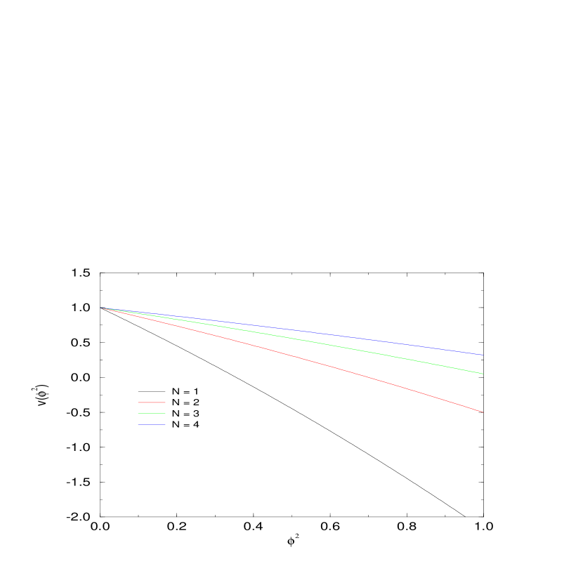
Figure 2.2: The perturbation corresponding to $\nu$ at leading order in the derivative expansion, for three dimensional $O(N)$ symmetric field theory, for $N=1,2,3,4$.

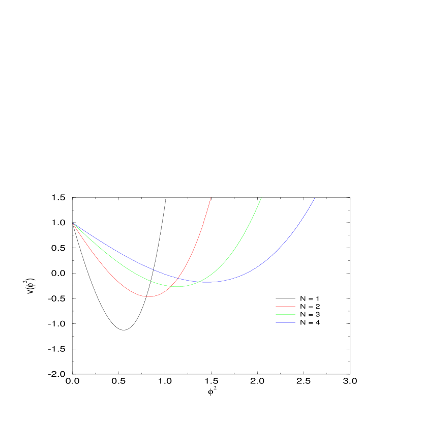
Figure 2.3: The perturbation corresponding to $\omega$ leading order in the derivative expansion for three dimensional $O(N)$ symmetric field theory, for $N=1,2,3,4$.

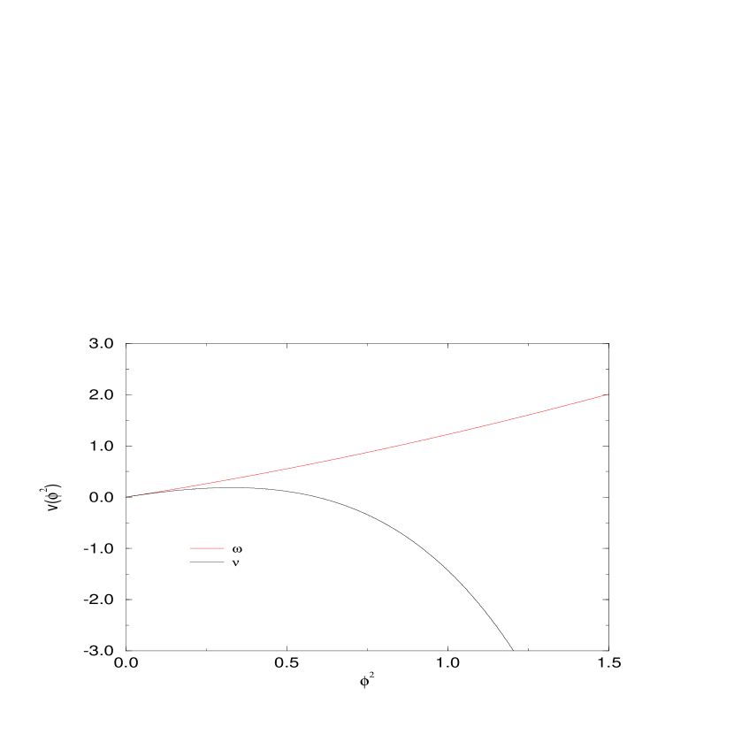
Figure 2.4: The perturbations corresponding to $\nu$ and $\omega$ at leading order in the derivative expansion for three dimensional $O(N)$ symmetric field theory, for $N=0$. The normalization condition is now given by $v^{\prime}(0)=1$.

Chapter 3 The Results at Second Order

In the previous chapter we showed how to obtain the results coming from the leading order of the approximation. In this chapter we will report the results of taking the approximation to the next order and including the effects of the terms involving two derivatives on the right hand side of the flow equation. This will lead to a vast increase in the complexity of the equations and the boundary conditions supplied to them. We will again specialize to the case $D=3$.

3.1 The Second Order Equations

Our starting point will again be equation (2.1), reproduced here,

$$(\frac{\partial}{\partial t}+D_{\phi}\Delta_{\phi}+\Delta_{\partial}-D)\Gamma[\phi]=$$

$$-\frac{1}{2\pi}\mathrm{tr}\int^{\infty}_{0}dqq^{D-1}\left(\frac{q}{C(q^{2})}\frac{\partial C(q^{2})}{\partial q}+2-\eta\right)\left\langle\left[\delta^{ab}+C_{.}\frac{\delta^{2}\Gamma}{\delta\phi^{a}\delta\phi^{b}}\right]^{-1}(\mathbf{q},-\mathbf{q})\right\rangle$$

We will again take $\Gamma[\phi]$ to be expanded as in equation (2.7). We will also force the coefficient functions to be non-singular for all $\phi^{2}$ at fixed points, and that the perturbations about these fixed points grow no faster than a power of $\phi^{2}$. The equations at the second order in the expansion are calculated by substituting expression (2.7) into equation (3.1) and dropping all terms with more than two derivatives from the right hand side. We will first consider what happens to the coefficient functions multiplying terms with more than two derivatives in them. We see that a general term $H(\phi^{2},t)$ will satisfy,

$$\frac{\partial}{\partial t}H(\phi^{2},t)+(1+\eta)(\phi^{2}H^{\prime}(\phi^{2},t)+n_{\phi}H(\phi^{2},t))+n_{\partial}H(\phi^{2},t)-3H(\phi^{2},t)=0$$ (3.2)

where $n_{\phi}$ denotes the number of $\phi^{a}$’s in the term multiplying $H$ divided by 2 and $n_{\partial}$ is the number of derivatives in the term multiplying $H$. We can no longer force that $\eta$ be zero at fixed points, and this leads to the following expression for $H$ at fixed points (setting D=3),

$$H\propto\phi^{-\frac{(1+\eta)n_{\phi}+n_{\partial}-3}{1+\eta}}$$ (3.3)

Hence, as $n_{\phi}>2$ and $n_{\partial}>2$, we see that $H$ will be singular at the origin, under mild assumptions about $\eta$, eg $\eta>0$. We are therefore forced to set all the terms with more than two derivatives in them equal to zero. Hence at the second order of the derivative expansion we parameterize $\Gamma$ as follows,

$$\Gamma[\phi^{2}]=\int d^{D}x\left\{V(\phi^{2},t)+\frac{1}{2}K(\phi^{2},t)\left(\partial_{\mu}\phi^{a}\right)^{2}+\frac{1}{2}Z(\phi^{2},t)\left(\phi^{a}\partial_{\mu}\phi^{a}\right)^{2}\right\}$$ (3.4)

A little bit of thought shows that this conclusion holds at all orders in the approximation: if we substitute an expression into the equation that is of higher order than the order we are working at, then we are forced to set the higher order terms to zero [30].

The next step is to compute the inverse in equation (3.1). This is not as straightforward as in the leading order case and a more involved technique is required. The steps that are required will depend upon the value of $N$: the case of $N=1$ is slightly different than the more general case. We discuss the more general case first before briefly reporting the results at $N=1$.

We will regard $[\delta^{ab}+C.\delta^{2}\Gamma/\delta\phi^{a}\delta\phi^{b}]^{-1}$ as a differential operator:

$$\left[\delta^{ab}+C.\frac{\delta^{2}\Gamma}{\delta\phi^{a}\phi^{b}}\right]^{-1}\!\!\!(\mathbf{q},\mathbf{-q}) = \int d^{D}x\,d^{D}y\,\mathrm{e}^{-i\mathbf{q.x}}\left[\delta^{ab}+C.\frac{\delta^{2}\Gamma}{\delta\phi^{a}\delta\phi^{b}}\right]^{-1}\!\!\!(\mathbf{x},\mathbf{y})\,\mathrm{e}^{i\mathbf{q.y}}$$ (3.5)

$$\equiv \int d^{D}x\,Q^{ab}$$

$$\mbox{where}\ \ \ \ \ \ \ \ \ \ \ \ \ \ Q^{ab} = \mathrm{e}^{-i\mathbf{q.x}}\left[\delta^{ab}+C.\frac{\delta^{2}\Gamma}{\delta\phi^{a}\delta\phi^{b}}\right]^{-1}\!\!\!\mathrm{e}^{i\mathbf{q.x}}$$ (3.6)

$Q^{ab}$ is a function of $\mathbf{q}$ and $\phi(\mathbf{x})$ and its derivatives evaluated at $\mathbf{x}$. To calculate $Q^{ab}$ we will regard $C$ and $\frac{\delta^{2}\Gamma}{\delta\phi^{a}\delta\phi^{b}}$ as differential operators. Noting that we are performing a derivative expansion, we should expect $Q^{ab}\approx(\delta^{ab}+\nu^{ab})^{-1}+\cdots$, where $\nu^{ab}$ is the expression obtained by dropping all terms containing differentials of $\phi^{a}$ from $C(q^{2})\mathrm{e}^{-i\mathbf{q.x}}\frac{\delta^{2}\Gamma}{\delta\phi^{a}\delta\phi^{b}}\mathrm{e}^{i\mathbf{q.x}}$. Hence noting that

$$Q^{ac}\left(\delta^{cb}+\nu^{cb}\right)=\left(\delta^{ac}+\nu^{ac}\right)\left[(\delta^{cb}+\nu^{cd})^{-1}Q^{db}+(\delta^{cd}+\nu^{cd})^{-1}\nu^{de}Q^{eb}\right]$$ (3.7)

and that from (3.6) we have,

$$Q^{ab}=\delta^{ab}-\mathrm{e}^{-i\mathbf{q.x}}C(-\Box)\frac{\delta^{2}\Gamma}{\delta\phi^{a}\delta\phi^{c}}\mathrm{e}^{i\mathbf{q.x}}Q^{cb}$$ (3.8)

we must have $Q^{ab}$ satisfying the following expression,

$$Q^{ab}=(\delta^{ab}+\nu^{ab})^{-1}+(\delta^{ac}+\nu^{ac})^{-1}\left\{\nu^{cd}Q^{cb}-\mathrm{e}^{-i\mathbf{q.x}}C(-\Box)\frac{\delta^{2}\Gamma}{\delta\phi^{c}\delta\phi^{d}}\mathrm{e}^{i\mathbf{q.x}}Q^{db}\right\}$$ (3.9)

The derivative expansion is performed by iterating expression (3.9) to the required order, here up to two derivatives, starting with $Q^{ab}=1/(\delta^{ab}+\nu^{ab})$, and remembering that $C(-\Box)=-\Box$. To do this we must calculate $\frac{\delta^{2}\Gamma}{\delta\phi^{a}\delta\phi^{b}}$, which is found, after a long but straightforward calculation, to be,

$$\frac{\delta^{2}\Gamma}{\delta\phi^{a}\delta\phi^{b}} = 4\phi^{a}\phi^{b}V^{\prime}+2\delta^{ab}V^{\prime}$$ (3.10)

$$-\delta^{ab}K\Box-2(\Box\phi^{a})\phi^{b}K^{\prime}$$

$$-2\delta^{ab}(\phi^{c}\partial_{\mu}\phi^{c})^{2}K^{\prime}\partial_{\mu}-2(\partial_{\mu}\phi^{a})(\partial_{\mu}\phi^{b})K^{\prime}$$

$$-2(\partial_{\mu}\phi^{a})\phi^{b}K^{\prime}\partial_{\mu}-4(\partial_{\mu}\phi^{a})\phi^{b}(\phi^{c}\partial_{\mu}\phi^{c})^{2}K^{\prime}$$

$$+2\phi^{a}(\partial_{\mu}\phi^{b})K^{\prime}\partial_{\mu}+\delta^{ab}(\partial_{\mu}\phi^{c})^{2}K^{\prime}$$

$$+2\phi^{a}\phi^{b}(\partial_{\mu}\phi^{c})^{2}K^{\prime}$$

$$-\delta^{ab}(\partial_{\mu}\phi^{c})^{2}Z-2\phi^{a}(\partial_{\mu}\phi^{b})Z\partial_{\mu}$$

$$-2\phi^{a}\phi^{b}(\partial_{\mu}\phi^{c})^{2}Z^{\prime}-\delta^{ab}(\phi^{c}\Box\phi^{c})Z$$

$$-\phi^{a}(\Box\phi^{b})Z-\phi^{a}\phi^{b}Z\Box$$

$$-2\phi^{a}\phi^{b}(\phi^{c}\Box\phi^{c})Z^{\prime}-\delta^{ab}(\phi^{c}\partial_{\mu}\phi^{c})^{2}Z^{\prime}$$

$$-2\phi^{a}(\partial_{\mu}\phi^{b})(\phi^{c}\partial_{\mu}\phi^{c})^{2}Z^{\prime}-2\phi^{a}\phi^{b}(\phi^{c}\partial_{\mu}\phi^{c})Z^{\prime}\partial_{\mu}$$

$$-2\phi^{a}\phi^{b}(\phi^{c}\partial_{\mu}\phi^{c})^{2}Z^{\prime}$$

This expression is then used in (3.9) to iterate $Q^{ab}$ to two derivatives. This is an extremely long calculation and was performed using the symbolic manipulation package Form [62]. The only remaining step is to calculate the trace over the spin indices. This will require the calculation of $(\delta^{ab}+\nu^{ab})^{-1}$, and the derivative of its inverses. This is easily done by noting that if $\delta^{ab}+\nu^{ab}=A+B\phi^{a}\phi^{b}$ then,

$$(\delta^{ab}+\nu^{ab})^{-1}=\frac{\delta^{ab}}{A}-\frac{B}{A(A+B\phi^{2})}\phi^{a}\phi^{b}$$ (3.11)

and also by noting that if we have a matrix $A(x)$ then $\frac{dA^{-1}}{dx}=-A^{-1}\frac{dA}{dx}A^{-1}$.

This calculation then yields the following equation for $V$, near fixed points,

$$\frac{\partial}{\partial t}V+(1+\eta)\phi^{2}V^{\prime}-3V=-\left(1-\eta/4\right)\times$$

$$\left[\frac{N-1}{\sqrt{K}\left(2V^{\prime}+2\sqrt{K}\right)^{1/2}}+\frac{1}{\sqrt{K+\phi^{2}Z}\left(2V^{\prime}+4\phi^{2}V^{\prime\prime}+2\sqrt{K+\phi^{2}Z}\right)^{1/2}}\right]$$

we refer to the above equation as the $V$ equation. Similarly the equations coming from the $(\partial_{\mu}\phi^{a})^{2}$ and $(\phi^{a}\partial_{\mu}\phi^{a})^{2}$ parts of the action will be referred to as the $K$ and $Z$ equations respectively. The equations for $K$ and $Z$ are a lot longer and are relegated to an appendix. We will perform one further transformation on the equations. To enable an easier comparison with the $N=\infty$ equation we will scale the equations as follows,

$$\phi = N\tilde{\phi}$$ (3.13)

$$V = N\tilde{V}$$ (3.14)

$$K = \tilde{K}$$ (3.15)

$$Z = \tilde{Z}/N$$ (3.16)

This then yields the following equation for $V$,

$$\frac{\partial}{\partial t}V+(1+\eta)\phi^{2}V^{\prime}-3V=-\left(1-\eta/4\right)\times$$

$$\!\!\!\!\left[\frac{1}{N\sqrt{K+\phi^{2}Z}\left(2V^{\prime}+4\phi^{2}V^{\prime\prime}+2\sqrt{K+\phi^{2}Z}\right)^{1/2}}+\frac{1-1/N}{\sqrt{K}\left(2V^{\prime}+2\sqrt{K}\right)^{1/2}}\right]$$

where we have dropped the tildes on $V$, $K$ and $Z$.

3.2 The Fixed Points Solutions

To find the fixed points we will again need to consider the boundary conditions supplied to the equations. We will again ensure that the solutions exist at the origin by imposing the equation at the origin. This will provide three conditions. We can also perform the asymptotic analysis as in the previous chapter. Once more we find that either the solution is the trivial Gaussian fixed point ($\eta=0,V=N/3\sqrt{2},K=1,Z=0$), that the solutions are only defined for $\phi^{2}<\phi_{c}^{2}$, or that the solutions behave as follows as $\phi^{2}\rightarrow\infty$,

$$V(\phi^{2}) \sim \mathit{A_{v}}\ (\phi^{2})^{\frac{3}{1+\eta}}+\cdots$$ (3.18)

$$K(\phi^{2}) \sim \mathit{A_{k}}\ (\phi^{2})^{\frac{-\eta}{1+\eta}}+\cdots$$ (3.19)

$$Z(\phi^{2}) \sim \mathit{A_{z}}\ (\phi^{2})^{\frac{-(1+2\eta)}{1+\eta}}+\cdots$$ (3.20)

We will be most interested in the non-trivial solutions defined for all $\phi^{2}$. We can also study the perturbations about these solutions. Forcing the perturbations to grow no faster than a power, we see that the solutions satisfying (3.18) to (3.20) will form a discrete set, with the solutions parameterized by the values of $\mathit{A_{v}}$, $\mathit{A_{k}}$ and $\mathit{A_{z}}$.

At the moment the value of $\eta$ as been left undetermined and it appears that we have a free parameter. However we can use the scaling symmetry to impose an extra condition and hence fix this extra parameter. We will take $K(0)=1$, with other possible solutions being reached by using the re-parameterization invariance. We now have a seven parameter set with seven conditions imposed and hence expect at most a discrete set of solutions. Again we only find two:- the Gaussian point mentioned above and an approximation to the Wilson-Fisher fixed point. The results for $\eta$ are summarized in table (3.1) and the results for the fixed point solutions shown in figures (3.1) to (3.3).

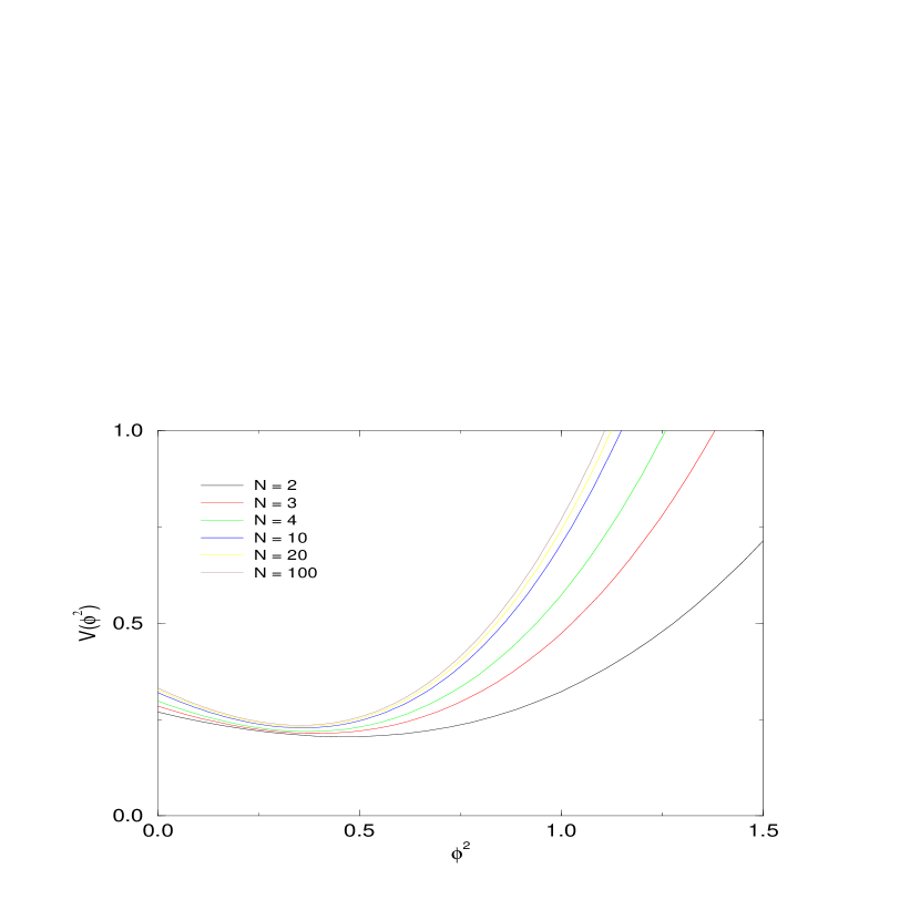
Figure 3.1: The Legendre effective potential at second order in the derivative expansion, for three dimensional $O(N)$ symmetric field theory, for $N=2,3,4,10,20,100$.

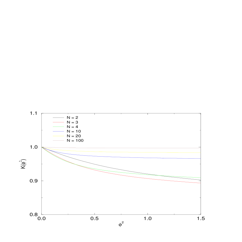
Figure 3.2: The K component of the wave function renormalization of the Legendre effective action at second order in the derivative expansion, for three dimensional $O(N)$ symmetric field theory, for $N=2,3,4,10,20,100$.

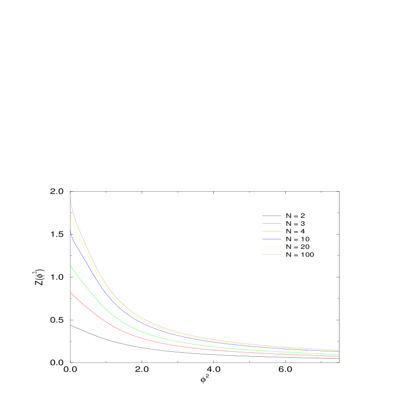
Figure 3.3: The Z component of the wave function renormalization of the Legendre effective action at second order in the derivative expansion, for three dimensional $O(N)$ symmetric field theory, for $N=2,3,4,10,20,100$.

3.3 The Critical Exponents at Second Order

To calculate the critical exponents we will again need to consider the perturbations about the fixed point solutions. That is we will write,

$$V(\phi^{2},t) = V^{*}(\phi^{2})+\delta V(\phi^{2},t)$$ (3.21)

$$= V^{*}(\phi^{2})+\varepsilon\mathrm{e}^{\lambda t}v(\phi^{2})$$

$$K(\phi^{2},t) = K^{*}(\phi^{2})+\delta K(\phi^{2},t)$$ (3.22)

$$= K^{*}(\phi^{2})+\varepsilon\mathrm{e}^{\lambda t}k(\phi^{2})$$

$$Z(\phi^{2},t) = Z^{*}(\phi^{2})+\delta Z(\phi^{2},t)$$ (3.23)

$$= Z^{*}(\phi^{2})+\varepsilon\mathrm{e}^{\lambda t}z(\phi^{2})$$

where $V^{*}(\phi^{2})$, $K^{*}(\phi^{2})$, $Z^{*}(\phi^{2})$ are the fixed point solutions calculated above, and expand the equations to first order in $\varepsilon$.

To find the perturbations we will again need to consider the boundary conditions. We will want the perturbations to exist for all $\phi^{2}$. If we insist that $v$,$k$ and $z$ grow no faster that a power at large $\phi^{2}$, then asymptotic analysis will show that $v$, $k$ and $z$ will grow according to their scaling dimension,

$$v(\phi^{2}) \sim \mathit{a_{v}}(\phi^{2})^{\frac{3}{1+\eta}-\lambda}+\cdots$$ (3.24)

$$k(\phi^{2}) \sim \mathit{a_{k}}(\phi^{2})^{\frac{-\eta}{1+\eta}-\lambda}+\cdots$$ (3.25)

$$z(\phi^{2}) \sim \mathit{a_{z}}(\phi^{2})^{-\frac{1+2\eta}{1+\eta}-\lambda}+\cdots$$ (3.26)

The imposition of power law growth will again force $\mathit{a_{v}}$, $\mathit{a_{k}}$ and $\mathit{a_{z}}$ to form an isolated three parameter set. The other three boundary conditions come from forcing the equations to hold at the origin. Using linearity to set $v(0)=1$, we will have a seven parameter set with seven boundary conditions imposed. Hence we expect to find at most a discrete set of solutions, which is what is found. As before we find just one positive eigenvalue, which yields $\nu$ through $\nu=1/\lambda$, and determine the least negative eigenvalue, which gives the first correction to scaling exponent through $\omega=-\lambda$. These values are shown in table (3.1).

It is important to recognize that we will also find other solutions of the equations which do not correspond to critical indices [63]. These solutions are known as redundant perturbations and the eigenvalue corresponding to the solution depends on the exact form of the renormalization group chosen, but as their eigenvalue depends on the exact form of the equation chosen these perturbations can not be physical. The redundant perturbation reflect invariances of the equations. In general if we change variables $\phi^{a}(x)=\tilde{\phi}^{a}(x)+\varepsilon\Phi^{a}[\tilde{\phi}]$ in (3.1) (with $J.\phi$ replaced by $J.\tilde{\phi}$), then this induces a change in the effective action of $\delta\Gamma=F.\frac{\delta\Gamma}{\delta\phi}$ with $F[\phi]=\varepsilon\exp\left(-W[J]\right)\Phi[\delta/\delta J]\exp\left(W[J]\right)$ and a change in the cutoff functional [30, 63]. A general choice of $F$ that will leave (2.7) invariant at this order is,

$$F[\phi]=\left\{f(\phi^{2}(x))\phi^{a}+\alpha x^{\mu}\partial_{\mu}\phi^{a}(x)\right\}$$ (3.27)

for any function $f$ and any constant $\alpha$. A redundant perturbation must then satisfy,

$$v \propto 2f\phi^{2}V^{\prime}-3\alpha V$$ (3.28)

$$k \propto 2f\phi^{2}K^{\prime}+2fK-\alpha K$$ (3.29)

$$z \propto 2f\phi^{2}Z^{\prime}+4f^{\prime}\phi^{2}Z+4fZ-\alpha Z+2f^{\prime}K$$ (3.30)

In fact we expect and find only one redundant perturbation corresponding to the re-parameterization invariance (2.8). This has eigenvalue $\lambda=0$, $f=5/2\alpha$ and $\alpha\neq 0$, yielding $(v,k,z)=(-5\phi^{2}V^{\prime}+3V,-5\phi^{2}K^{\prime}-4K,-5\phi^{2}Z^{\prime}-9Z)$, where we have set $\alpha=-1$. An obvious question is why no redundant perturbations are found at the leading order. The answer is simple: the choice of $K\equiv 1$ breaks the re-parameterization invariance, and we should not expect to see any redundant perturbation. We should also not expect to see any perturbation corresponding to $\phi$-translation invariance [41] as the choice of $V,K$ and $Z$ being functions of $\phi^{2}$ breaks this invariance.

The redundant perturbation also proves to be a convenient check on the numerical accuracy of the equations for the perturbations. Once we know the fixed point solutions we automatically know a solution to the perturbation equation, which should have eigenvalue $\lambda=0$. We can then try to find our redundant solution using numerical methods. The degree to which the known solution (from the fixed points), and the solution found numerically agree, gives a bound on the accuracy of the critical exponents. Using numerical methods, we find that the value for the eigenvalue corresponding to the redundant perturbation typically lies in the range $0.0003$ (for $N=2$) to $0.00005$ (for $N=100$), indicating that we should only trust any numeric results to three figures. The graphs of the two types of solutions also agree to a high degree of accuracy.

3.4 The case of $N=1$

As mentioned above the case of $N=1$ is slightly different to the more general case of $N\neq 1$. This should not be entirely surprising as there is now no internal symmetry at all (other than the discrete $Z_{2}$ symmetry). The derivative expansion now becomes,

$$\Gamma[\phi]=\int d^{D}x\left\{V(\phi^{2})+\frac{1}{2}\left(K(\phi^{2})+\phi^{2}Z(\phi^{2})\right)\left(\partial_{\mu}\phi\right)^{2}\right\}$$ (3.31)

We see that we should no longer consider the $Z$ and $K$ components of wave function renormalization separately, but should consider instead a single function $\kappa=K+\phi^{2}Z$. The derivative expansion at second order, at $N=1$, thus becomes,

$$\Gamma[\phi]=\int d^{D}x\left\{V(\phi^{2})+\frac{1}{2}\kappa(\phi^{2})\left(\partial_{\mu}\phi\right)^{2}\right\}$$ (3.32)

We will no longer have three coupled second order equations but will have only two coupled second order equations for $V$ and $\kappa$. The results for this case can be found in [30]. It is an important check on our equations that if we write $\kappa=K+\phi^{2}Z$ and set $N=1$, then we get the same equations as found in [30]. The results of this expansion are included in figure (3.4) for completeness. These come from an independent calculation.

(a) $V(\phi^{2})$

(b) $\kappa(\phi^{2})$

Figure 3.4: The results of applying the derivative expansion at second order for the case of $N=1$.

It is interesting to ask what does happen to the $K$ and $Z$ components as $N\rightarrow 1$. This can be done by taking the $K$ equation and substituting $K=\kappa-\phi^{2}Z$ into it. This then yields an equation which can be solved numerically using the known result for $\kappa$ and $V$ (from [30] or our independent calculation). It is then found, that at $N=1$, $Z$ diverges as $1/\phi^{2}$ at the origin. Again this should not be entirely surprising: we can write $Z=(\kappa-K)/\phi^{2}$, and should therefore expect to see some divergence at the origin, provided $K(0)\neq\kappa(0)$. Numerically this is an important point. As $N\rightarrow 1$ we will expect that $Z$ will become steeper and steeper at the origin before it eventually becomes divergent at $N=1$. This divergent behavior may lead to numerical instability as we approach the regime $N\approx 1$. In fact we start to feel the effects of this divergence as early as $N=2$, where it is already found to be much harder to produce an accurate numerical solution than at $N=3$, say.

$N$	$\eta$		$\nu$			$\omega$
	$O(\partial^{2})$		$O(\partial^{2})$	$O(\partial^{0})$		$O(\partial^{2})$	$O(\partial^{0})$
1	0.054	0.035	0.62	0.66	0.63	0.898	0.63	0.80
2	0.044	0.033 - 0.04	0.65	0.73	0.67	0.38	0.66	0.79
3	0.035	0.033 - 0.04	0.745	0.78	0.71	0.33	0.71	0.78
4	0.022	0.025	0.816	0.8240	0.75	0.42	0.75
10	0.0054	0.025	0.95	0.93	0.88	0.82	0.89	0.78
20	0.0021	0.013	0.98	0.96	0.94	0.93	0.95	0.89
100	0.00034	0.003	0.998	0.994	0.989	0.988	0.991	0.98

Table 3.1: Critical exponents of the three-dimensional theory for various values of $N$. We list the results gained at second order together with those from the leading order and an indication of what should be expected from other methods as summarized in [22, 56, 58, 57]. $\eta$ is predicted to be zero for all $N$ at the leading order in the approximation.

3.5 Discussion

The results at second order are puzzling: for $N=2,3,4$ we have reasonable accuracy for $\eta$ and $\nu$, with an improvement upon the leading order results, but terrible predictions for $\omega$, which is predicted to be worse than the leading order results. On the other hand the predictions at $N=10,20,100$ show the converse: we have $\eta$ seriously underestimated, by a factor of about ten, and the results for $\nu$ compare less favourably with other methods than those predicted by the leading order of the approximation. However we also see an improvement in the predictions for $\omega$ compared to other methods.

These results are very puzzling as the only other comparable calculations at this order in the derivative expansion [30, 64], performed at $N=1$, showed an improvement for all the calculated exponents when the change was made from the leading order to the second order of the derivative expansion. Other authors who have tried to go beyond the leading order of the approximation certainly do not report results for $\omega$ like those we have found at $N=2,3,4$ [61]. It would be easy to explain these results away by calling upon numerical inaccuracy, especially at $N=2,3,4$ where the known steep behaviour of $Z$ at the origin may have an effect. However, although it is true that the equations are extremely difficult to solve (cf appendix A) we feel that this is unlikely for several reasons. Firstly the results are insensitive to changes in where we impose the asymptotic boundary condition, the number of points in the solution mesh and other numerical factors, whereas we might expect there to be random errors introduced if the results were down to numerical roundoff or discretization error. For example, it can be seen that the eigenvalues seem to flow continuously with the value of N, whereas we would perhaps expect some random fluctuations if we were encountering severe numerical problems. Secondly, we already know that the known redundant perturbation can be found to a reasonable degree of accuracy, indicating that we should have a high degree of faith in our numerical methods and in the numerical stability of the equations themselves. For these two reasons it seems rather unlikely that these effects are due to numerical problems.

Figure 3.5: The flow of $\eta$ and $\omega$ with the value of $N$. Figure b also shows what the large $N$ expansion predicts at order $1/N$.

Quite why the results do not compare so well with those presented by others is puzzling. The serious under-prediction of $\eta$ for large $N$ could be attributed to the approximation scheme being ’too biased’ towards the $N=\infty$ results, which would predict $\eta=0$, at large $N$. It is also interesting to note that the flow of $\omega$ with $N$ seems to follow the large $N$ results at order $1/N$ for $N=3,4,5,\ldots...$. The results of these two flows are shown in figure (3.5).

Overall we must conclude that the scheme for intermediate $N$ does not work as well as it does for $N=1$ or $N=\infty$. The $N=\infty$ result is in fact exact and is well understood (cf the next chapter and [41]). The reason why the encouraging results at $N=1$ [30, 64] are not continued for $N\neq 1$ are not yet understood. However, it should be emphasized that we find no evidence for spurious results, such as those found by truncations: we find only the fixed points and perturbations expected.

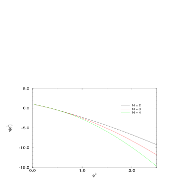
(a) $v(\phi^{2})$

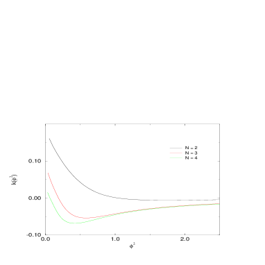
(b) $k(\phi^{2})$

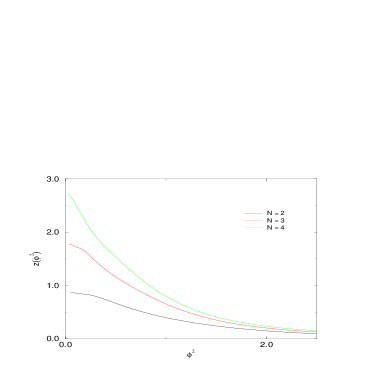
(c) $z(\phi^{2})$

Figure 3.6: The $v$, $k$ and $z$ components of the perturbation corresponding to $\nu$ at second order in the derivative expansion

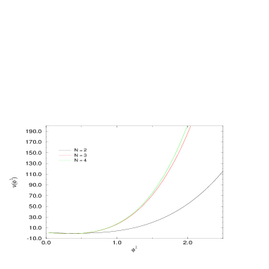
(a) $v(\phi^{2})$

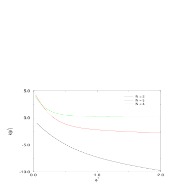
(b) $k(\phi^{2})$

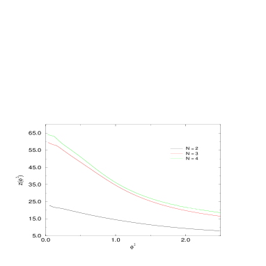
(c) $z(\phi^{2})$

Figure 3.7: The $v$, $k$ and $z$ components of the perturbation corresponding to $\omega$ at second order in the derivative expansion

Chapter 4 Exactly Solvable Systems

It has been well known that certain theoretical models can be exactly solved. That is, have all their physical parameters determined without any form of approximation. In this section we will discuss how the derivative expansion reproduces the exact results found in two well known cases:– $N=\infty$ and $N=-2$. It is important that the derivative expansion reproduces these two exactly known results, for if it didn’t then the approximation would be too great a mutilation of the theory.

4.1 Exact Results at $N=\infty$

It was noted a long time ago that the large $N$ limit is equivalent [65] to the exactly solvable spherical model [66]. It was shown that in the large $N$-limit that the local potential expansion effectively becomes exact. ie we have,

$$\Gamma[\phi]\equiv\int d^{D}x\,\frac{1}{2}\left(\partial_{\mu}\phi^{a}\right)^{2}+V(\phi^{2})\ \ \ \ \mbox{at $N=\infty$}$$ (4.1)

In this section we will show that the derivative expansion re-produces this result and give an expression for $V(\phi^{2})$ and for the perturbations about the fixed point.

In the previous chapter we scaled the equations to provide a comparison with the $N=\infty$ results. We now justify where these scalings come from.

We will consider a simple scalar $\Phi^{4}$ theory in $D$ dimensions,

$$Z = \int D\Phi\exp\left\{-S[\Phi]+\int d^{D}xJ.\Phi\right\}$$ (4.2)

$$S[\Phi] = \int d^{D}x\,\frac{1}{2}(\partial_{\mu}\Phi)^{2}+\frac{m^{2}}{2}\Phi^{2}+\frac{u}{4!}[\Phi^{2}]^{2}$$ (4.3)

We can perform the following transformation

$$\exp-\frac{u}{4!}\int d^{D}x\,[\Phi^{2}]^{2}\sim\int D\lambda\exp\left\{\int d^{D}x\frac{N\lambda^{2}}{2}-\frac{\lambda}{2}\Phi^{2}\sqrt{\frac{Nu}{3}}\right\}$$ (4.4)

and hence re-write the path integral as,

$$Z=\int D\lambda\exp\left\{\int d^{D}x\,\left(\frac{1}{2}N\lambda^{2}\right)+\frac{N}{2}\mathrm{tr}\log\left({-\Delta+m^{2}+\sqrt{\frac{Nu}{3}}\lambda}\right)\right\}$$ (4.5)

We see from this that we now have an explicit dependence on $N$ in the (non-local) action. If we wish to perform a saddle point expansion in $1/N$ then we must have a factor of $N$ outside the action, but none in the $\mathrm{tr}\log$. From this we see that we must hold $Nu$ fixed, so $u$ is of order $1/N$, and we must have $\lambda$ of order one also. Hence, counting the powers of $N$ in equation (4.4) and demanding that the powers of $N$ match up on both sides, we see that we must have $\Phi^{2}$ of order $N$.

From this we see that when we come to consider the flow equations we should scale $\phi^{2}$ as $\phi^{2}=N\tilde{\phi^{2}}$. Hence, demanding that $\Gamma$ scales as $\Gamma=N\tilde{\Gamma}$ (as follows from (4.5), we have the following scalings,

$$V \sim N\tilde{V}$$ (4.6)

$$K \sim \tilde{K}$$ (4.7)

$$Z \sim \tilde{Z}/N$$ (4.8)

where $\tilde{V}$,$\tilde{K}$ and $\tilde{Z}$ are of order one in the $1/N$ expansion. Upon doing this the flow equation for $V$ becomes (upon dropping the tildes),

$$\frac{\partial}{\partial t}V+(1+\eta)\phi^{2}V^{\prime}-3V=-\left(1-\eta/4\right)\times$$

$$\left[\frac{1}{N\sqrt{K+\phi^{2}Z}\left(2V^{\prime}+4\phi^{2}V^{\prime\prime}+2\sqrt{K+\phi^{2}Z}\right)^{1/2}}+\frac{1-1/N}{\sqrt{K}\left(2V^{\prime}+2\sqrt{K}\right)^{1/2}}\right]$$

plus some longer equations for $K$ and $Z$. If we now take the $N=\infty$ limit we end up with the following sets of equations,

$$\frac{\partial}{\partial t}V+(1+\eta)\phi^{2}V^{\prime}-3V = -\frac{\left(1-\eta/4\right)}{\sqrt{K}\left(2V^{\prime}+\sqrt{K}\right)^{1/2}}$$ (4.10)

$$\frac{\partial}{\partial t}K+(1+\eta)\phi^{2}K^{\prime}+\eta K = -\frac{(1-\eta/4)K^{\prime}}{\sqrt{K}\left(2V^{\prime}+2\sqrt{K}\right)^{3/2}}$$ (4.11)

$$\frac{\partial}{\partial t}Z+(1+\eta)\phi^{2}Z^{\prime}+(1+2\eta)Z = \cdots$$ (4.12)

We immediately notice something different:- the equations for $K$ and $V$ have decoupled from the equation for $Z$ and the equations are now first order equations. This is the first simplification.

Now lets consider the fixed point solutions. The next simplification comes by looking at the local potential expansion and noting that this will require that $K\equiv 1$. Hence we try $K\equiv 1$ as a fixed point solution. Equation (4.11) then yields, $\eta=0$.

Upon setting $\eta=0$ we find that the fixed point potentials will then satisfy,

$$\phi^{2}V^{\prime}-3V=-\frac{1}{\left(2V^{\prime}+2\right)^{1/2}}$$ (4.13)

Although this is a first order equation it is still not in a particularly useful form for solution. If we differentiate the equation with respect to $\phi^{2}$ and set $W(\phi^{2})=V^{\prime}(\phi^{2})$ then we have,

$$-2W+\phi^{2}W^{\prime}=\frac{W^{\prime}}{(2+2W)^{3/2}}$$ (4.14)

This equation can the be re-arranged as partial differential equation for $\phi^{2}$ in $W$ as follows,

$$2W\frac{\partial\phi^{2}}{\partial W}-\phi^{2}=-\frac{1}{(2+2W)^{3/2}}$$ (4.15)

Using $1/\sqrt{W}$ as an integrating factor we then have,

$$\frac{\partial\frac{\phi^{2}}{\sqrt{W}}}{\partial W}=-\frac{1}{2W^{3/2}(2+2W)^{3/2}}$$ (4.16)

Performing the final integration then yields a final expression for $\phi^{2}$,

$$\phi^{2}=A\sqrt{W}+\frac{1}{2\sqrt{2}}\sqrt{1+W}\left(1+\frac{W}{1+W}\right)$$ (4.17)

where $A$ is a constant of integration. If we have $A\neq 0$ then it can be shown that $\phi^{2}$ will reach a maximum value for some non zero value of $W$. ie the solution is not defined for all values of $\phi^{2}$. We are therefore required to set $A=0$ and the solution then becomes,

$$\phi^{2}=\frac{1}{2\sqrt{2}}\sqrt{1+W}\left(1+\frac{W}{1+W}\right)$$ (4.18)

This can be inverted to give the solution for $W$,

$$W=-1+\left[\frac{1}{\sqrt{2}}\phi^{2}+\frac{1}{\sqrt{2}}\sqrt{(\phi^{2})^{2}+1}\right]^{2}$$ (4.19)

Integrating with respect to $\phi^{2}$ then gives the solution for the potential,

$$V=-\frac{1}{2}\phi^{2}+\frac{(\phi^{2})^{3}}{3}+\frac{((\phi^{2})^{2}+1)^{3/2}}{3}$$ (4.20)

It is important to stress the difference between the scaled and the unscaled results in the large $N$ regime. The unscaled $V$ tends to infinity, $K$ tends to $1$ and $Z$ tends to zero as $N\rightarrow\infty$. However when we consider the scaled solutions we see a different pattern: $V$ now tends to our solution (4.20), $K$ still tends to one, but so far $Z$ has been left undetermined.

Performing the scaling upon the $Z$ equation and setting $K=1,K^{\prime}=0$ we see that $Z$ must satisfy the following equation,

$$\phi^{2}Z^{\prime}+Z=$$

$$-{{\it i}_{2,0,2}}\,{\it Z^{\prime}}+{\displaystyle\frac{32}{3}}{\phi^{2}}\,{\it V^{\prime\prime}}{\displaystyle\frac{1024}{3}}\,{{\it i}_{4,3,2}}\,{\it V^{\prime\prime}}^{4}\,{(\phi^{2})}^{2}$$

$$+\left(\!\,4\,{{\it i}_{6,2,3}}-8\,{{\it i}_{4,2,3}}+{{\it i}_{4,2,2}}+4\,{{\it i}_{2,2,3}}-5\,{{\it i}_{2,2,2}}+{{\it i}_{2,2,1}}\,\!\right)\,{\it V^{\prime\prime\prime}}$$

$$+{\displaystyle\frac{64}{3}}{\phi^{2}}\left({\vrule height=5.29999pt,width=0.0pt,depth=5.29999pt}\right.\!\!16\,{{\it i}_{5,3,2}}\,{Z}\,{\phi^{2}}-8\,{{\it i}_{5,2,3}}-11\,{{\it i}_{3,2,2}}\mbox{}+8\,{{\it i}_{3,2,3}}-8\,{{\it i}_{3,3,2}}$$

$$+8\,{{\it i}_{3,3,1}}+8\,{{\it i}_{5,3,2}}\!\!\left.{\vrule height=5.29999pt,width=0.0pt,depth=5.29999pt}\right){\it V^{\prime\prime}}^{3}\mbox{}$$

$$+\left({\vrule height=7.89993pt,width=0.0pt,depth=7.89993pt}\right.\!\!\mbox{}{\displaystyle\frac{256}{3}}\,{\phi^{2}}\,{Z}\,{{\it i}_{6,3,2}}-{\displaystyle\frac{256}{3}}\,{\phi^{2}}\,{Z}\,{{\it i}_{4,3,2}}+{\displaystyle\frac{256}{3}}\,{\phi}^{2}\,{Z}\,{{\it i}_{4,2,3}}$$

$$\mbox{}-{\displaystyle\frac{416}{3}}\,{\phi^{2}}\,{Z}\,{{\it i}_{4,2,2}}+{\displaystyle\frac{256}{3}}\,{(\phi^{2})}^{2}\,{Z}^{2}\,{{\it i}_{6,3,2}}+{\displaystyle\frac{128}{3}}\,{{\it i}_{6,2,3}}-{\displaystyle\frac{256}{3}}\,{{\it i}_{4,2,3}}$$

$$\mbox{}-64\,{{\it i}_{4,2,2}}+{\displaystyle\frac{128}{3}}\,{{\it i}_{2,2,3}}-{\displaystyle\frac{64}{3}}\,{{\it i}_{2,2,2}}-{\displaystyle\frac{64}{3}}\,{{\it i}_{2,2,1}}+{\displaystyle\frac{128}{3}}\,{{\it i}_{6,0,5}}$$

$$\mbox{}+{\displaystyle\frac{64}{3}}\,{{\it i}_{6,3,2}}+{\displaystyle\frac{128}{3}}\,{{\it i}_{4,3,1}}-{\displaystyle\frac{128}{3}}\,{{\it i}_{6,1,4}}+{\displaystyle\frac{256}{3}}\,{{\it i}_{4,1,4}}+{\displaystyle\frac{80}{3}}\,{{\it i}_{4,1,3}}$$

$$\mbox{}+{\displaystyle\frac{128}{3}}\,{{\it i}_{2,0,5}}+{\displaystyle\frac{16}{3}}\,{{\it i}_{2,0,3}}-32\,{{\it i}_{2,0,4}}+{\displaystyle\frac{64}{3}}\,{{\it i}_{2,3,0}}+{\displaystyle\frac{64}{3}}\,{{\it i}_{2,3,2}}$$

$$\mbox{}-{\displaystyle\frac{128}{3}}\,{{\it i}_{2,1,4}}+{\displaystyle\frac{112}{3}}\,{{\it i}_{2,1,3}}+{\displaystyle\frac{16}{3}}\,{{\it i}_{2,1,2}}-{\displaystyle\frac{128}{3}}\,{{\it i}_{2,3,1}}-{\displaystyle\frac{32}{3}}\,{{\it i}_{4,0,4}}$$

$$\mbox{}-{\displaystyle\frac{256}{3}}\,{{\it i}_{4,0,5}}-{\displaystyle\frac{128}{3}}\,{{\it i}_{4,3,2}}\!\!\left.{\vrule height=7.89993pt,width=0.0pt,depth=7.89993pt}{\displaystyle\frac{256}{3}}\,{\phi^{2}}\,{Z}\,{{\it i}_{4,3,1}}-{\displaystyle\frac{256}{3}}\,{\phi^{2}}\,{Z}\,{{\it i}_{6,2,3}}\right){\it V^{\prime\prime}}^{2}\mbox{}$$

$$+\left({\vrule height=7.89993pt,width=0.0pt,depth=7.89993pt}\right.\!\!\mbox{}{\displaystyle\frac{8}{3}}\,{\phi}^{2}\,{\it Z^{\prime}}\,{{\it i}_{3,2,1}}+{\displaystyle\frac{8}{3}}\,{Z}\,{{\it i}_{5,2,2}}-{\displaystyle\frac{40}{3}}\,{\phi^{2}}\,{\it Z^{\prime}}\,{{\it i}_{3,2,2}}-{\displaystyle\frac{64}{3}}\,{\phi^{2}}\,{\it Z^{\prime}}\,{{\it i}_{5,2,3}}$$

$$\mbox{}-{\displaystyle\frac{40}{3}}\,{Z}\,{{\it i}_{3,2,2}}+{\displaystyle\frac{8}{3}}\,{Z}\,{{\it i}_{3,2,1}}+{\displaystyle\frac{32}{3}}\,{Z}\,{{\it i}_{3,2,3}}-{\displaystyle\frac{64}{3}}\,{Z}\,{{\it i}_{5,2,3}}$$

$$\mbox{}+{\displaystyle\frac{32}{3}}\,{\phi^{2}}\,{\it Z^{\prime}}\,{{\it i}_{7,2,3}}+8\,{Z}\,{{\it i}_{3,0,3}}+{\displaystyle\frac{32}{3}}\,{Z}\,{{\it i}_{7,2,3}}+{\displaystyle\frac{32}{3}}\,{\phi^{2}}\,{\it Z^{\prime}}\,{{\it i}_{3,2,3}}$$

$$\mbox{}+\,{\displaystyle\frac{8}{3}}\,{\phi^{2}}\,{\it Z^{\prime}}\,{{\it i}_{5,2,2}}\!\!\left.{\vrule height=7.89993pt,width=0.0pt,depth=7.89993pt}\right){\it V^{\prime\prime}}$$

where $i_{j,k,m}$ represents the following integral,

$$\int d^{D}q\frac{q^{2j}}{\left(1+(2V^{{}^{\prime}}+4\phi^{2}V^{{}^{\prime\prime}})q^{2}+(1+\phi^{2}Z)q^{4}\right)^{k}\left(1+2V^{{}^{\prime}}q^{2}+q^{4}\right)^{m}}$$

(a) $V(\phi^{2})$

(b) $Z(\phi^{2})$

Figure 4.1: The potential, $V$, and the Z component of the wave function renormalization of the Legendre effective action at second order in the derivative expansion, at $N=\infty$.

Of course this equation can no longer be solved analytically, as above, but the numerical solution is straightforward. Imposing the constraint that $Z$ exists for all $\phi^{2}$ we get the solution shown in figure (4.1b).

We have now calculated what the fixed point potentials look like, but what we are really interested in is the critical exponents. To calculate these we will again linearize about the fixed point solutions by writing $V(\phi^{2},t)=V^{*}(\phi^{2})+\varepsilon\mathrm{e}^{\lambda t}v(\phi^{2})$ and $K(\phi^{2},t)=K^{*}(\phi^{2})+\varepsilon\mathrm{e}^{\lambda t}k(\phi^{2})$, where $V^{*}$ and $K^{*}$ denote the fixed point solutions found above. Using these expressions in equations (4.10) and (4.11) and expanding to first order in $\varepsilon$ yields the following pair of differential equations,

$$\lambda v+\phi^{2}v^{\prime}-3v = \frac{1}{2}\frac{k+2v^{\prime}}{(2+2V^{\prime})^{3/2}}$$ (4.21)

$$\lambda k+\phi^{2}k^{\prime} = \frac{k^{\prime}}{(2V^{\prime}+2)^{3/2}}$$ (4.22)

We will consider equation (4.22) first. Re-arranging the equation we have,

$$\frac{k^{\prime}}{k}=-\frac{\lambda(2V^{\prime}+2)^{3/2}}{\phi^{2}(2V^{\prime}+2)^{3/2}-1}$$ (4.23)

Using expression (4.20) we then have,

$$\frac{k^{\prime}}{k}=-\frac{\lambda\left\{2(\phi^{2})^{2}+1+2\phi^{2}\sqrt{(\phi^{2})^{2}+1}\right\}^{3/2}}{\phi^{2}\left\{2(\phi^{2})^{2}+1+2\phi^{2}\sqrt{(\phi^{2})^{2}+1}\right\}^{3/2}-1}$$ (4.24)

This can easily integrated to give the solution for $k(\phi^{2})$,

$$A_{1}\left(\mathrm{e}^{2\sinh^{-1}\phi^{2}}-2\right)^{-\lambda/2}$$ (4.25)

where $A_{1}$ is a constant of integration.

We now consider the $v$ equation. This can be re-written as follows,

$$\frac{(\lambda-3)(2+2V^{\prime})^{3/2}v}{\phi^{2}(2+2V^{\prime})^{3/2}-1}+v^{\prime}=\frac{1}{2}\frac{k}{\phi^{2}(2+2V^{\prime})^{3/2}-1}$$ (4.26)

Using an integrating factor of $(\exp(2\sinh^{-1}\phi^{2})-2)^{\lambda/2-3/2}$, this equation becomes,

$$\frac{d}{d\phi^{2}}\left(v(\phi^{2})\,(\exp(2\sinh^{-1}\phi^{2})-2)^{\lambda/2-3/2}\right)=\frac{1}{2}\frac{k\;(\exp(2\sinh^{-1}\phi^{2})-2)^{\lambda/2-3/2}}{\phi^{2}(2+2V^{\prime})^{3/2}-1}$$ (4.27)

Using the known results for $V(\phi^{2})$ and $k(\phi^{2})$ this equation can be integrated to give,

$$A_{1}\frac{1}{12}\left(2\mathrm{e}^{3\sinh^{-1}\phi^{2}}-6\mathrm{e}^{\sinh^{-1}\phi^{2}}+3\mathrm{e}^{-\sinh^{-1}\phi^{2}}\right)\left(\mathrm{e}^{2\sinh^{-1}\phi^{2}}-2\right)^{-\lambda/2}$$

$$+A_{2}\left(\mathrm{e}^{2\sinh^{-1}\phi^{2}}-2\right)^{3/2-\lambda/2}$$ (4.28)

From equation (4.25) we note that for $k(0)$ to be real we need $\lambda=-2m$, where $m$ is an integer, or have $A_{1}=0$. However, we also note that to avoid a singularity near the origin we must have $m$ positive or zero ( as $\exp(2\sinh^{-1}\phi^{2})-2<0$ for $\phi^{2}<\sinh(\log\sqrt{2})$). On the other hand, considering equation (4.28) we see that we must also have $3/2-\lambda/2$ to be a positive integer, or have $A_{2}=0$. We see that we must have two mutually exclusive sets of solutions:-

• a set of solutions with eigenvalues $\lambda=3-2m$, for a positive integer $m$, and $A_{1}=0$. These solutions have $\lambda=3,1,-1,\ldots$ and satisfy

  $$v(\phi^{2}) = A_{2}\left(\mathrm{e}^{2\sinh^{-1}\phi^{2}}-2\right)^{3/2-\lambda/2}$$ (4.29)

  $$k(\phi^{2}) = 0$$ (4.30)

• a set of solutions with $A_{2}=0$ and $\lambda=-2m$, for a positive integer $m=0,1,2,3$. These solutions have $\lambda=0,-2,-4,\ldots$ and satisfy,

  $$v(\phi^{2}) = A_{1}\frac{1}{12}\left(2\mathrm{e}^{3\sinh^{-1}\phi^{2}}-6\mathrm{e}^{\sinh^{-1}\phi^{2}}+3\mathrm{e}^{-\sinh^{-1}\phi^{2}}\right)$$ (4.31)

  $$\ \ \ \ \ \times\left(\mathrm{e}^{2\sinh^{-1}\phi^{2}}-2\right)^{-\lambda/2}$$

  $$k(\phi^{2}) = A_{1}\left(\mathrm{e}^{2\sinh^{-1}\phi^{2}}-2\right)^{-\lambda/2}$$ (4.32)

The first set of results reproduce those first found by Wegner and Houghton [41], whilst the second set correspond to corrections to scaling coming from the $(\partial_{\mu}\phi^{a})^{2}$ part of the action. We plot some of these functions for various values of $\lambda$ in figure (4.2). It should be noted that all the solutions meet at the point $(0,1/2\sqrt{2})$. This behaviour is related to the singularity structure of the equations and is not of any particular importance.

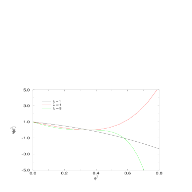
(a) $v(\phi^{2})$ for the first type of solution

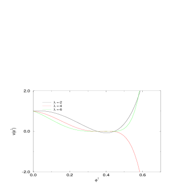
(b) $v(\phi^{2})$ for the second type of solution

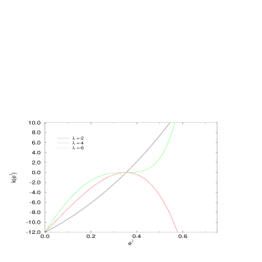
(c) $k(\phi^{2})$ for the second type of solution

Figure 4.2: The $v$ and $k$ components of the relevant, leading irrelevant and sub-leading irrelevant operators at $N=\infty$.

4.2 Exact Results at $N=-2$

The fact that the case of $N=-2$ is also an exactly solvable case was noted long ago [67, 68]. The initial hope was to be able to combine the known results at $N=\infty$ with the new results at $N=-2$, and use Padé approximants to gain information about the physically interesting case of $N=0,1,2,3$ [67, 68, 69]. It was found that when $N=-2$ the exponents reduce to those of the Gaussian model, $\eta=0$, $\nu=1/2$. However there is one large difference: the $N=-2$ case describes the critical Gaussian model, as opposed to the tricritical Gaussian model [70]. Therefore, we only expect to find one relevant eigenvalue instead of the two relevant eigenvalues that we found in section 2.3.1.

This phenomena can be understood as follows. As pointed out by Fisher [68], at $N=-2$ only the quadratic part of the action plays a role, ie the physics is totally independent of any quartic coupling etc. At the tricritical fixed point we see two relevant operators corresponding to a mass term with dimension two and a $\phi^{4}$ term with dimension one. However, as we are now reduced to only having the quadratic part of the action playing a rôle, we only can expect to find one relevant operator.

We will show how the derivative expansion reproduces these results at the leading order of the approximation before briefly discussing what happens when we consider the second order terms.

Our starting point will be the equation for the potential at leading order,

$$\phi^{2}V^{\prime}-3V=-\left\{\frac{N-1}{\sqrt{2+2V^{\prime}}}+\frac{1}{\sqrt{2+2V^{\prime}+4\phi^{2}V^{\prime\prime}}}\right\}$$ (4.33)

It turns out that we need only consider what happens at the origin. If we differentiate the equation and set $\phi^{2}=0$ we get,

$$-\frac{N+2}{(2+2V^{\prime}(0))^{3/2}}V^{\prime\prime}(0)-2V^{\prime}(0)$$ (4.34)

We see that at $N=-2$ this equation simplifies to $-2V^{\prime}(0)=0$, so we must have $V^{\prime}(0)=0$. Considering equation (4.33) at $\phi^{2}=0$ we see that we must then have $V(0)=-\sqrt{2}/3$. From this we see an interesting departure of the behaviour at the origin from the cases $N=1,2,3,\ldots$, etc. Beforehand the boundary condition at the origin used to leave $V(0)$ and $V^{\prime}(0)$ as free parameters, constrained by the given boundary condition. However we now have $V(0)$ and $V^{\prime}(0)$ exactly determined, with $V^{\prime\prime}(0)$ decoupling and becoming a free parameter. The question is whether we can find a non-trivial solution: after all if $V^{\prime\prime}(0)=0$ then series methods show that we only reproduce the tricritical Gaussian solution, $V(\phi^{2})=N/(3\sqrt{2})$. All analytic attempts to find such a solution failed, but if we use $V(0)=-\sqrt{2}/3$ and $V^{\prime}(0)=0$ as boundary conditions then numerical methods quickly find a non-trivial solution with $V^{\prime\prime}(0)\neq 0$ satisfying the required asymptotic conditions at large $\phi^{2}$ (cf equation (2.21)). The results of this search are shown in figure (4.3a).

We now consider what happens to $v(\phi^{2})$. We consider the linearized equation,

$$(\lambda-3)v+\phi^{2}v^{\prime}=\frac{(N-1)v^{\prime}}{(2+2V^{\prime})^{3/2}}+\frac{v^{\prime}+\phi^{2}v^{\prime\prime}}{(2+2V^{\prime}+4\phi^{2}V^{\prime\prime})^{3/2}}$$ (4.35)

If we differentiate this equation and set $\phi^{2}=0$ we have,

$$-\frac{(N+2)v^{\prime\prime}}{(2V^{\prime}+2)^{3/2}}+3\frac{(N+2)v^{\prime}V^{\prime\prime}}{(2V^{\prime}+2)^{5/2}}+v^{\prime}(\lambda-2)$$ (4.36)

Hence we see that if we set $N=-2$ then the terms involving $V^{\prime\prime}$ and $v^{\prime\prime}$ decouple and we are left with,

$$v^{\prime}(\lambda-2)=0$$ (4.37)

(a) The fixed point potential, $V(\phi^{2})$

(b) The perturbation $v(\phi^{2})$ for $\lambda=2$.

Figure 4.3: The fixed point solution for the critical-Gaussian fixed point, together with the only found perturbation, at $N=-2$.

Therefore, we either have $\lambda=2$ or we must take $v^{\prime}(0)=0$. Hence we see that we find the first eigenvalue without re-course to any analytic or numerical method, and so $\nu=1/2$. Again we check numerically that we find a solution that isn’t just the tricritical Gaussian solution. This is shown in figure (4.3b). If we take $v^{\prime}(0)=0$, then setting $\phi^{2}=0$ in the linearized equation at $N=-2$, shows that $v(0)=0$. We now have a second order equation with two boundary conditions set at the origin and hence we expect to find a unique result. By inspection we see that this solution must be $v(\phi^{2})=0$.

As pointed out by Fisher [68] we should also expect to find exact solutions for $N=-4,-6-8,\ldots$. We find this to be the case. eg consider $N=-4$, following a similar method to above, except this time differentiating twice, yields,

$$2\sqrt{2}\frac{(\lambda-1)(\lambda-2)v^{\prime}(0)}{N+2}$$ (4.38)

From this we see that we must have $\lambda=2$ or $\lambda=1$ or have $v^{\prime}(0)=0$. As before the case of $v^{\prime}(0)=0$ yields no further results. This result should be expected because, as Fisher pointed out [68], at $N=-4$ interactions up to degree $\phi^{4}$ now play a rôle. The program can be carried out for any negative even integer to yield similar results, so for $N=-6$ we have $\lambda=2,1,0$ and interactions up to degree $\phi^{6}$ become involved.

When we come to perform the analysis at the second order the equations are vastly more complicated. Due to the fact that even modern symbolic manipulation packages cannot handle the equations efficiently we report no further results.

Appendix A Numerical methods

In this section we will outline the methods used to solve our equations. We begin with the numerical methods used before discussing particular problems that we encountered.

A.1 Numerical Methods

The equations form a two point boundary value problem. There are two such methods of solving such equations: shooting [76, 77] and relaxation [77]. Both methods were used at some point in the research.

A.1.1 Shooting

Suppose we have a set $N$ of differential equations,

$$\frac{dy_{i}(x)}{dx}=g_{i}(x,y_{1},\ldots,y_{N})\ \ \ \ \ \ \ \ i=1,2,\ldots,N$$ (A.1)

with two boundary conditions. At the first boundary, $x=x_{1}$ the solution is supposed to satisfy,

$$B_{j}(x_{1},y_{1},\ldots,y_{N})=0\ \ \ \ \ \ \ \ j=1,\ldots,n_{1}$$ (A.2)

whilst at the second, $x=x_{2}$ it is supposed to satisfy,

$$\tilde{B}_{j}(x_{2},y_{1},\ldots,y_{N})=0\ \ \ \ \ \ \ \ j=1,\ldots,n_{2}$$ (A.3)

with $n_{1}+n_{2}=N$.

In the shooting method we choose a set of values for all the dependent values at the first boundary. These values are chosen to be consistent with the boundary condition (A.2), but are otherwise free to depend upon a set of free parameters, the values of which we guess. Using the values of the dependent variables as initial conditions we integrate equation (A.1) out to the second boundary, using a standard ordinary differential equation integrator. Of course we will usually find that there is a discrepancy in how well the values at the second boundary fit the boundary condition there. How well the values at the second boundary condition fit the boundary condition depend upon the initial choice of the dependent variables, so we now have a problem of finding what initial values of the dependent variables fit the second boundary condition the best. Hence, the problem has been reduced to a multi-dimensional root finding problem which can be solved using any of the standard methods of numerical analysis (eg Newton-Raphson etc).

A.1.2 Relaxation

In the relaxation method the equations are replaced by a finite difference mesh that spans the range that we are interested in. An initial guess is then supplied: this guess need not satisfy the equation or even the the boundary conditions. An iteration process known as relaxation is then performed to bring the equations into closer agreement with the finite difference equations and the boundary conditions. This again boils down to solving a multi-dimensional set of non-linear equations using some numerical method.

Relaxation is particularly suited to equations and boundary conditions involving complicated expressions which can’t be solved in closed form. ie there is no need to explicitly write the equation in the form $dy/dx=f(x,y)$. It is also the best method when we need to find solutions that depend upon some parameter, such as the value of $N$ in our $O(N)$ symmetry. Once we have found a solution for one value of $N$ we can use this solution as an initial guess for a close value of $N$. Given the nature of our problem it is not surprising that relaxation turns out to be the principal method used during the research.

A.2 The Boundary Conditions

Before discussing the solutions of the equations it is necessary to discuss the equations and the boundary conditions supplied to them.

We wish to formulate the equations as a set of non-linear, coupled second order differential equations. Noting that the equation relating to the $Z$ part of the action contains powers of $V^{\prime\prime\prime}$ (cf appendix B) it is necessary to differentiate the $V$ equation and find an expression for $V^{\prime\prime\prime}$ in terms of $V,V^{\prime},V^{\prime\prime},K,K^{\prime},Z$ and $Z^{\prime}$. Similarly, when we come to look at the boundary condition relating to the $Z$ equation we see that it contains powers of $V^{\prime\prime}$. Again we differentiated the $V$ equation to find an expression for $V^{\prime\prime}(0)$ in terms of $V,V^{\prime},K$ and $Z$. Similar transformations where made when we determined the equations for the perturbations.

The other set of boundary conditions seem to be more problematic. We need the solutions to exist for all $\phi^{2}$. We know that if the solutions exist for all $\phi^{2}$ then we can work out how the solutions behave at large $\phi^{2}$. This is what provides the second boundary condition. We choose a value of $\phi^{2}$ such that the asymptotic expressions (shown in appendix B) become a good enough approximation to the solutions. We then use the asymptotic expressions for $V,K$ and $Z$ to provide boundary conditions for $V,V^{\prime},K,K^{\prime},Z$ and $Z^{\prime}$. The value of $\phi^{2}$ chosen, which we call $\phi^{2}_{\mathrm{asy}}$, must be chosen large enough to ensure that the solutions satisfy the asymptotic conditions sufficiently well, but not so large that numerical instability prevents us from obtaining a solution. There is a certain amount of trial and error in deciding where to set $\phi^{2}_{\mathrm{asy}}$: we cannot really decide where to set it until we know something about the solution. The solutions were also checked to be stable against reasonable changes in the value of $\phi^{2}_{\mathrm{asy}}$.

In fact it is necessary to develop the asymptotic expressions to beyond the leading order in order to find a solution. eg consider equation (2.20), if we just use the leading order results, where the solutions behave according to their scaling dimension, then we see that, as we set $\phi^{2}_{\mathrm{asy}}$ at a finite value, then $V^{\prime\prime}(\phi^{2})$ would be left undetermined. Hence, we are forced to expand the asymptotic expressions to beyond leading order. A similar result holds for $K(\phi^{2})$. However, when we consider $Z(\phi^{2})$, we see that we need to take the asymptotic expressions to next to next to leading order. This is because when we calculate the correction to the leading order asymptotic behaviour it does not involve $Z^{\prime\prime}$, hence leaving $Z^{\prime\prime}$ undetermined. In order to ensure that $Z^{\prime\prime}$ gets determined, we need to extend the asymptotic expression to one further order.

When we come to consider the perturbed equations it is sufficient to use the leading order asymptotic expression. As a check we calculated the corrections to the leading order behaviour and also used these. This made no difference to the values quoted.

A.3 The Solution of the Equations

Having determined the boundary conditions we can discuss how the numerical solution of the equations was performed. The solution of the equations is complicated by the fact that they are stiff [76, 77]. This arises because small perturbations from the true solutions lead to a singular behaviour. Relaxation is particularly adept at handling stiff problems. Before discussing these issues we briefly discuss the problems posed by the integrals in the equations.

A.3.1 The Integrals $I_{a,b,c}$

The integrals $I_{a,b,c}$ play an important part in the solution. Defined by,

$$I_{a,b,c}=\int_{0}^{\infty}\frac{q^{2a}\,dq}{\left(1+(2V^{\prime}+4\phi^{2}V^{\prime\prime})q^{2}+(K+\phi^{2}Z)q^{4}\right)^{b}\left(1+2V^{\prime}q^{2}+Kq^{4}\right)^{c}}$$

it is possible to find a general analytic result for them. This proves not to be a sensible thing to do. The integrals are generally small numbers, but in the analytic expressions these small numbers arise from the cancellation of two large numbers. Roundoff errors start to play a large part in determining their value using the analytic expression. Even performing the calculations using higher precision Fortran routines could not provide accuracy beyond four significant figures. This level of accuracy was totally insufficient and so numerical methods were used.

We used an adaptive integrator from the NAG libraries. The problem was split into two parts: a part from zero up to some finite value, and the remaining bit. To avoid roundoff errors we used an expression arising from asymptotic analysis to calculate the second part of the integral, and only used the numerical routines in the part of the real line from the origin. The point were the crossover took place was set to be as small as possible (to avoid numeric round off in the numerical integration), whilst still allowing the asymptotic expression to be accurate.

A.3.2 The $Z$ equation at $N=\infty$

The equation that determines $Z$ at $N=\infty$, equation (4.1) is a first order non-linear equation. Being first order we only have one boundary condition, which is that the solution exists for all $\phi^{2}$ and has the required asymptotic behaviour. For this problem we used the shooting method. An initial value of $Z$ was used to integrate the equation out towards the second boundary using an eight point Runge-Kutta integrator. In general the initial value of $Z$ would be wrong: if it was too large then the solution would tend to infinity at some finite $\phi^{2}$; if it was too small the solution would tend to minus infinity at some finite value of $\phi^{2}$. Using a binary chop we could home into the correct value of $Z(0)$ and find the solution that was defined for all $\phi^{2}$.

It was particularly difficult to get past the point $\phi^{2}=1/2\sqrt{2}$. This is because at this point the right hand side of the equations has a $0/0$ type behaviour. ie if $Z^{\prime}=n(\phi^{2},Z)/d(\phi^{2},Z)$, then as $\phi^{2}\rightarrow 1/2/\sqrt{2}$ we see that $n(\phi^{2},Z)\rightarrow 0$ and $d(\phi^{2},Z)\rightarrow 0$, for the true solution. There are general methods of dealing with such singular points [77], but our equations were sufficiently well behaved to avoid needing to use them.

A.3.3 The Numerical Solution of the Flow Equations for General $N$

The numerical solution of the leading order equations proved to be easy. It was only necessary to provide an initial guess and the relaxation routines quickly found the solution.

When we come to consider the second order equations we see that there is vast increase in the complexity of the equations. The numerical solution of the second order equation is made difficult by the large number of integrals that need to be calculated during each iteration. This places a huge computational overhead on the numerical calculations. It was soon noted that the computational power required could not be provided by normal machines. Parallel Fortran code, making use of MPI [78], was developed to run on a sixteen node IBM SP2 system. The use of a parallel machine considerably speeded the calculation up, with run times typically between ten minutes to one hour (before developing parallel code the programs could take up to one week to run). Using the $N=\infty$ solutions as an initial guess allowed us to solve the general $N$ cases using relaxation.

The shooting method was tried, but this proved to be unsuitable. This is because to use shooting effectively we need to be able to reach the other boundary or have a particularly simple set of equations (eg the $N=\infty$ equations). The singularity structure of the equations makes it impossible to shoot from one side to the other and hence makes the more complicated problem unsuited to shooting.

The main difficultly in solving the second order equation was removing the instabilities in $Z$ near the origin. These manifested themselves in the form of sharp spikes in $Z^{\prime}$ near $\phi^{2}=0$. These were removed by writing $Z(\phi^{2})=s(\phi^{2})\tilde{Z}(\phi^{2})$, where $s(\phi^{2})$ is a known scaling function that makes $\tilde{Z}(\phi^{2})$ as flat as possible. This greatly speeded up the calculations and removed the spikes in the solutions.

When we came to consider the equations for the perturbations it was realized that we could calculate the parts that relied upon the fixed point solutions and store them in a file, thus saving a large computational overhead. It was important that these functions, which are the functions that multiplied $v,v^{\prime},v^{\prime\prime},k$ etc in each of the linearized equations, are well determined. The size of the $z$ equation was such that small errors in the fixed point solutions made it difficult to determine these functions accurately, for large $\phi^{2}$ . This problem was solved by noting that we could determine these functions by using the known asymptotic expressions for $V,K$ and $Z$ and then matching them onto the ones calculated from the fixed point solutions. It was checked that the eigenvalues were stable against reasonable perturbations in where $\phi^{2}_{\mathrm{asy}}$ was set and the number of points in the mesh.

Appendix B The Equations at Second Order

In this appendix we show some of the expressions thought to too long to appear in the main body of the text. We include the equations for $K$ and $Z$ as well as the expressions for the asymptotics to next to leading order.

B.1 The Second Order Equations

In the the expression below $I_{a,b,c}$ represents the following integral,

$$I_{a,b,c}=\int_{0}^{\infty}\frac{q^{2a}dq}{\left(1+(2V^{\prime}+4\phi^{2}V^{\prime\prime})q^{2}+(K+\phi^{2}Z)q^{4}\right)^{b}\left(1+2V^{\prime}q^{2}+Kq^{4}\right)^{c}}$$

These integrals are not evaluated as the equations become very large. At present there are about three hundred terms in the equations. Evaluating the integrals raises this to between twenty five and thirty thousand terms.

The $K$ equation is given by

$${\it(1+\eta)\phi^{2}K^{\prime}+\eta K=}$$

$$\frac{(\,4-{\eta}\,)}{\pi}\left[{\vrule height=8.00003pt,width=0.0pt,depth=8.00003pt}\right.\!\!{\it I}_{4,2,1}\,\left(\!\,{\displaystyle\frac{4}{3}}\,{\displaystyle\frac{{\it K^{\prime}}^{2}\,{\phi}}{{N}}}+{\displaystyle\frac{4}{3}}\,{\displaystyle\frac{{\it K^{\prime}}\,{Z}\,{\phi}}{{N}}}\,\!\right)\mbox{}+{\it I}_{4,1,2}\,\left(\!\,{\displaystyle\frac{4}{3}}\,{\displaystyle\frac{{\it K^{\prime}}^{2}\,{\phi}}{{N}}}-4\,{\displaystyle\frac{{\it K^{\prime}}\,{Z}\,{\phi}}{{N}}}+{\displaystyle\frac{8}{3}}\,{\displaystyle\frac{{Z}^{2}\,{\phi}}{{N}}}\,\!\right)$$

$$\mbox{}+{\displaystyle\frac{16}{3}}\,{\displaystyle\frac{{\it I}_{3,2,1}\,{\it V^{\prime\prime}}\,{\it K^{\prime}}\,{\phi}}{{N}}}+{\it I}_{3,1,2,}\,\left(\!\,-\,{\displaystyle\frac{16}{3}}\,{\displaystyle\frac{{\it V^{\prime\prime}}\,{\it K^{\prime}}\,{\phi}}{{N}}}+{\displaystyle\frac{16}{3}}\,{\displaystyle\frac{{\it V^{\prime\prime}}\,{Z}\,{\phi}}{{N}}}\,\!\right)$$

$$\mbox{}+{\it I}_{2,0,2}\,\left(\!\,{\displaystyle\frac{{\it K^{\prime}}}{{N}}}-{\displaystyle\frac{{Z}}{{N}}}-{\it K^{\prime}}\,\!\right)+{\it I}_{2,2,0}\,\left(\!\,-\,{\displaystyle\frac{{\it K^{\prime}}}{{N}}}-2\,{\displaystyle\frac{{\it K^{\prime\prime}}\,{\phi}}{{N}}}\,\!\right)\!\!\left.{\vrule height=8.00003pt,width=0.0pt,depth=8.00003pt}\right]$$

The longer $Z$ equation is given by,

$$(\,1+{\eta}\,)\,{\phi^{2}}\,{\it Z^{\prime}}+(\,1+2\,{\eta}\,)\,{Z}=$$

$${\displaystyle{\frac{(\,4-{\eta}\,)}{\pi}}\left[{\vrule height=8.6pt,width=0.0pt,depth=8.6pt}\right.\!\!}{{\it I}_{4,0,5}}\,\left(\!\,{\displaystyle\frac{256}{3}}\,{\displaystyle\frac{{\it V^{\prime\prime}}^{2}\,{K}}{{N}}}-{\displaystyle\frac{32}{3}}\,{\displaystyle\frac{{\it K^{\prime}}^{2}}{{N}}}-{\displaystyle\frac{256}{3}}\,{\it V^{\prime\prime}}^{2}\,{K}+{\displaystyle\frac{32}{3}}\,{\it K^{\prime}}^{2}\,\!\right)$$

$$+{{\it I}_{6,1,4}}\,\left(\!\,{\displaystyle\frac{128}{3}}\,{\displaystyle\frac{{\it V^{\prime\prime}}^{2}\,{K}^{2}}{{N}}}-{\displaystyle\frac{64}{3}}\,{\displaystyle\frac{{K}\,{\it K^{\prime}}^{2}}{{N}}}-{\displaystyle\frac{128}{3}}\,{\it V^{\prime\prime}}^{2}\,{K}^{2}+{\displaystyle\frac{64}{3}}\,{K}\,{\it K^{\prime}}^{2}\,\!\right)$$

$$+{{\it I}_{4,2,3}}\left({\vrule height=8.00003pt,width=0.0pt,depth=8.00003pt}\right.\!\!{\displaystyle\frac{256}{3}}\,{\displaystyle\frac{{\it V^{\prime\prime}}^{2}\,{K}}{{N}}}-{\displaystyle\frac{512}{3}}\,{\displaystyle\frac{{\it V^{\prime\prime}}^{2}\,{\it K^{\prime}}\,{\phi^{2}}}{{N}}}-{\displaystyle\frac{256}{3}}\,{\displaystyle\frac{{\it V^{\prime\prime}}^{2}\,{Z}\,{\phi^{2}}}{{N}}}$$

$$+{\displaystyle\frac{256}{3}}\,{\displaystyle\frac{{\it V^{\prime\prime}}\,{\it V^{\prime\prime\prime}}\,{K}\,{\phi^{2}}}{{N}}}-{\displaystyle\frac{16}{3}}\,{\displaystyle\frac{{\it K^{\prime}}\,{Z}}{{N}}}-{\displaystyle\frac{16}{3}}\,{\displaystyle\frac{{\it K^{\prime}}\,{\it Z^{\prime}}\,{\phi^{2}}}{{N}}}-{\displaystyle\frac{256}{3}}\,{\it V^{\prime\prime}}^{2}\,{K}$$

$$+{\displaystyle\frac{512}{3}}\,{\it V^{\prime\prime}}^{2}\,{\it K^{\prime}}\,{\phi^{2}}+{\displaystyle\frac{256}{3}}\,{\it V^{\prime\prime}}^{2}\,{Z}\,{\phi^{2}}-{\displaystyle\frac{256}{3}}\,{\it V^{\prime\prime}}\,{\it V^{\prime\prime\prime}}\,{K}\,{\phi^{2}}+{\displaystyle\frac{16}{3}}\,{\it K^{\prime}}\,{Z}$$

$$+{\displaystyle\frac{16}{3}}\,{\it K^{\prime}}\,{\it Z^{\prime}}\,{\phi^{2}}\!\!\left.{\vrule height=8.00003pt,width=0.0pt,depth=8.00003pt}\right)$$

$$+{{\it I}_{4,3,2}}\left({\vrule height=8.6pt,width=0.0pt,depth=8.6pt}\right.\!\!-\,{\displaystyle\frac{1024}{3}}\,{\displaystyle\frac{{\it V^{\prime\prime}}^{4}\,{(\phi^{2})}^{2}}{{N}}}+{\displaystyle\frac{128}{3}}\,{\displaystyle\frac{{\it V^{\prime\prime}}^{2}\,{K}}{{N}}}$$

$$+{\displaystyle\frac{512}{3}}\,{\displaystyle\frac{{\it V^{\prime\prime}}^{2}\,{\it K^{\prime}}\,{\phi^{2}}}{{N}}}+{\displaystyle\frac{256}{3}}\,{\displaystyle\frac{{\it V^{\prime\prime}}^{2}\,{Z}\,{\phi^{2}}}{{N}}}-{\displaystyle\frac{16}{3}}\,{\displaystyle\frac{{\it K^{\prime}}^{2}}{{N}}}+{\displaystyle\frac{1024}{3}}\,{\it V^{\prime\prime}}^{4}\,{(\phi^{2})}^{2}$$

$$-{\displaystyle\frac{128}{3}}\,{\it V^{\prime\prime}}^{2}\,{K}-{\displaystyle\frac{512}{3}}\,{\it V^{\prime\prime}}^{2}\,{\it K^{\prime}}\,{\phi^{2}}-{\displaystyle\frac{256}{3}}\,{\it V^{\prime\prime}}^{2}\,{Z}\,{\phi^{2}}+{\displaystyle\frac{16}{3}}\,{\it K^{\prime}}^{2}\!\!\left.{\vrule height=8.6pt,width=0.0pt,depth=8.6pt}\right)$$

$$+{{\it I}_{5,1,4}}\,\left(\!\,-\,{\displaystyle\frac{256}{3}}\,{\displaystyle\frac{{\it V^{\prime\prime}}\,{K}\,{\it K^{\prime}}}{{N}}}+{\displaystyle\frac{256}{3}}\,{\it V^{\prime\prime}}\,{K}\,{\it K^{\prime}}\,\!\right)$$

$$+{{\it I}_{4,2,1}}\left(\!\,{\displaystyle\frac{20}{3}}\,{\displaystyle\frac{{\it K^{\prime}}^{2}}{{N}}}-{\displaystyle\frac{8}{3}}\,{\displaystyle\frac{{\it K^{\prime}}\,{Z}}{{N}}}-{\displaystyle\frac{4}{3}}\,{\displaystyle\frac{{\it K^{\prime}}\,{\it Z^{\prime}}\,{\phi^{2}}}{{N}}}+{\displaystyle\frac{{Z}^{2}}{{N}}}-8\,{\it K^{\prime}}^{2}+{\displaystyle\frac{4}{3}}\,{\it K^{\prime}}\,{Z}+{\displaystyle\frac{4}{3}}\,{\it K^{\prime}}\,{\it Z^{\prime}}\,{\phi^{2}}\,\!\right)$$

$$+{{\it I}_{6,2,2}}\left({\vrule height=8.00003pt,width=0.0pt,depth=8.00003pt}\right.\!\!{\displaystyle\frac{56}{3}}\,{\displaystyle\frac{{K}\,{\it K^{\prime}}^{2}}{{N}}}-{\displaystyle\frac{4}{3}}\,{\displaystyle\frac{{K}\,{\it K^{\prime}}\,{Z}}{{N}}}-{\displaystyle\frac{4}{3}}\,{\displaystyle\frac{{K}\,{\it K^{\prime}}\,{\it Z^{\prime}}\,{\phi^{2}}}{{N}}}+{\displaystyle\frac{104}{3}}\,{\displaystyle\frac{{\it K^{\prime}}^{2}\,{Z}\,{\phi^{2}}}{{N}}}$$

$$-{\displaystyle\frac{56}{3}}\,{K}\,{\it K^{\prime}}^{2}+{\displaystyle\frac{4}{3}}\,{K}\,{\it K^{\prime}}\,{Z}+{\displaystyle\frac{4}{3}}\,{K}\,{\it K^{\prime}}\,{\it Z^{\prime}}\,{\phi^{2}}-{\displaystyle\frac{104}{3}}\,{\it K^{\prime}}^{2}\,{Z}\,{\phi^{2}}\!\!\left.{\vrule height=8.00003pt,width=0.0pt,depth=8.00003pt}\right)$$

$$+{{\it I}_{4,4,0}}\left({\vrule height=8.6pt,width=0.0pt,depth=8.6pt}\right.\!\!-144\,{\displaystyle\frac{{\it V^{\prime\prime}}^{2}\,{K}}{{N}}}-144\,{\displaystyle\frac{{\it V^{\prime\prime}}^{2}\,{Z}\,{\phi^{2}}}{{N}}}-192\,{\displaystyle\frac{{\it V^{\prime\prime}}\,{\it V^{\prime\prime\prime}}\,{K}\,{\phi^{2}}}{{N}}}-192\,{\displaystyle\frac{{\it V^{\prime\prime}}\,{\it V^{\prime\prime\prime}}\,{Z}\,{(\phi^{2})}^{2}}{{N}}}$$

$$-64\,{\displaystyle\frac{{\it V^{\prime\prime\prime}}^{2}\,{K}\,{(\phi^{2})}^{2}}{{N}}}-64\,{\displaystyle\frac{{\it V^{\prime\prime\prime}}^{2}\,{Z}\,{(\phi^{2})}^{3}}{{N}}}+4\,{\displaystyle\frac{{\it K^{\prime}}^{2}}{{N}}}+8\,{\displaystyle\frac{{\it K^{\prime}}\,{Z}}{{N}}}+8\,{\displaystyle\frac{{\it K^{\prime}}\,{\it Z^{\prime}}\,{\phi^{2}}}{{N}}}$$

$$+4\,{\displaystyle\frac{{Z}^{2}}{{N}}}+8\,{\displaystyle\frac{{Z}\,{\it Z^{\prime}}\,{\phi^{2}}}{{N}}}+4\,{\displaystyle\frac{{\it Z^{\prime}}^{2}\,{(\phi^{2})}^{2}}{{N}}}\!\!\left.{\vrule height=8.6pt,width=0.0pt,depth=8.6pt}\right)$$

$$+{{\it I}_{2,5,0}}\,\left(\!\,192\,{\displaystyle\frac{{\it V^{\prime\prime}}^{2}}{{N}}}+256\,{\displaystyle\frac{{\it V^{\prime\prime}}\,{\it V^{\prime\prime\prime}}\,{\phi^{2}}}{{N}}}+{\displaystyle\frac{256}{3}}\,{\displaystyle\frac{{\it V^{\prime\prime\prime}}^{2}\,{\phi^{2}}^{2}}{{N}}}\,\!\right)$$

$$+{{\it I}_{2,3,2}}\,\left(\!\,-\,{\displaystyle\frac{64}{3}}\,{\displaystyle\frac{{\it V^{\prime\prime}}^{2}}{{N}}}+{\displaystyle\frac{64}{3}}\,{\it V^{\prime\prime}}^{2}\,\!\right)$$

$$+{{\it I}_{2,3,1}}\,\left(\!\,{\displaystyle\frac{128}{3}}\,{\displaystyle\frac{{\it V^{\prime\prime}}^{2}}{{N}}}-{\displaystyle\frac{128}{3}}\,{\it V^{\prime\prime}}^{2}\,\!\right)$$

$$+{{\it I}_{4,1,4}}\,\left(\!\,-\,{\displaystyle\frac{256}{3}}\,{\displaystyle\frac{{\it V^{\prime\prime}}^{2}\,{K}}{{N}}}+{\displaystyle\frac{32}{3}}\,{\displaystyle\frac{{\it K^{\prime}}^{2}}{{N}}}+{\displaystyle\frac{256}{3}}\,{\it V^{\prime\prime}}^{2}\,{K}-{\displaystyle\frac{32}{3}}\,{\it K^{\prime}}^{2}\,\!\right)$$

$$+{{\it I}_{2,0,3}}\,\left(\!\,-\,{\displaystyle\frac{16}{3}}\,{\displaystyle\frac{{\it V^{\prime\prime}}^{2}}{{N}}}+{\displaystyle\frac{16}{3}}\,{\it V^{\prime\prime}}^{2}\,\!\right)$$

$$+{{\it I}_{5,2,3}}\left({\vrule height=8.00003pt,width=0.0pt,depth=8.00003pt}\right.\!\!{\displaystyle\frac{512}{3}}\,{\displaystyle\frac{{\it V^{\prime\prime}}^{3}\,{K}\,{\phi^{2}}}{{N}}}+{\displaystyle\frac{128}{3}}\,{\displaystyle\frac{{\it V^{\prime\prime}}\,{K}\,{\it K^{\prime}}}{{N}}}+{\displaystyle\frac{64}{3}}\,{\displaystyle\frac{{\it V^{\prime\prime}}\,{K}\,{Z}}{{N}}}+{\displaystyle\frac{64}{3}}\,{\displaystyle\frac{{\it V^{\prime\prime}}\,{K}\,{\it Z^{\prime}}\,{\phi^{2}}}{{N}}}$$

$$-{\displaystyle\frac{256}{3}}\,{\displaystyle\frac{{\it V^{\prime\prime}}\,{\it K^{\prime}}\,{Z}\,{\phi^{2}}}{{N}}}+{\displaystyle\frac{128}{3}}\,{\displaystyle\frac{{\it V^{\prime\prime\prime}}\,{K}\,{\it K^{\prime}}\,{\phi^{2}}}{{N}}}-{\displaystyle\frac{512}{3}}\,{\it V^{\prime\prime}}^{3}\,{K}\,{\phi^{2}}-{\displaystyle\frac{128}{3}}\,{\it V^{\prime\prime}}\,{K}\,{\it K^{\prime}}$$

$$-{\displaystyle\frac{64}{3}}\,{\it V^{\prime\prime}}\,{K}\,{Z}-{\displaystyle\frac{64}{3}}\,{\it V^{\prime\prime}}\,{K}\,{\it Z^{\prime}}\,{\phi^{2}}+{\displaystyle\frac{128}{3}}\,{\it V^{\prime\prime}}\,{\it K^{\prime}}^{2}\,{\phi^{2}}+{\displaystyle\frac{256}{3}}\,{\it V^{\prime\prime}}\,{\it K^{\prime}}\,{Z}\,{\phi^{2}}$$

$$-{\displaystyle\frac{128}{3}}\,{\it V^{\prime\prime\prime}}\,{K}\,{\it K^{\prime}}\,{\phi^{2}}-{\displaystyle\frac{128}{3}}\,{\displaystyle\frac{{\it V^{\prime\prime}}\,{\it K^{\prime}}^{2}\,{\phi^{2}}}{{N}}}\!\!\left.{\vrule height=8.00003pt,width=0.0pt,depth=8.00003pt}\right)$$

$$+{{\it I}_{8,0,5}}\,\left(\!\,-\,{\displaystyle\frac{32}{3}}\,{\displaystyle\frac{{K}^{2}\,{\it K^{\prime}}^{2}}{{N}}}+{\displaystyle\frac{32}{3}}\,{K}^{2}\,{\it K^{\prime}}^{2}\,\!\right)$$

$$+{{\it I}_{8,5,0}}\left({\vrule height=8.6pt,width=0.0pt,depth=8.6pt}\right.\!\!{\displaystyle\frac{16}{3}}\,{\displaystyle\frac{{K}^{2}\,{\it K^{\prime}}^{2}}{{N}}}+{\displaystyle\frac{32}{3}}\,{\displaystyle\frac{{K}^{2}\,{\it K^{\prime}}\,{Z}}{{N}}}+{\displaystyle\frac{32}{3}}\,{\displaystyle\frac{{K}^{2}\,{\it K^{\prime}}\,{\it Z^{\prime}}\,{\phi^{2}}}{{N}}}+{\displaystyle\frac{16}{3}}\,{\displaystyle\frac{{K}^{2}\,{Z}^{2}}{{N}}}$$

$$+{\displaystyle\frac{32}{3}}\,{\displaystyle\frac{{K}^{2}\,{Z}\,{\it Z^{\prime}}\,{\phi^{2}}}{{N}}}+{\displaystyle\frac{16}{3}}\,{\displaystyle\frac{{K}^{2}\,{\it Z^{\prime}}^{2}\,{(\phi^{2})}^{2}}{{N}}}+{\displaystyle\frac{32}{3}}\,{\displaystyle\frac{{K}\,{\it K^{\prime}}^{2}\,{Z}\,{\phi^{2}}}{{N}}}+{\displaystyle\frac{64}{3}}\,{\displaystyle\frac{{K}\,{\it K^{\prime}}\,{Z}^{2}\,{\phi^{2}}}{{N}}}$$

$$+{\displaystyle\frac{64}{3}}\,{\displaystyle\frac{{K}\,{\it K^{\prime}}\,{Z}\,{\it Z^{\prime}}\,{(\phi^{2})}^{2}}{{N}}}+{\displaystyle\frac{32}{3}}\,{\displaystyle\frac{{K}\,{Z}^{3}\,{\phi^{2}}}{{N}}}+{\displaystyle\frac{64}{3}}\,{\displaystyle\frac{{K}\,{Z}^{2}\,{\it Z^{\prime}}\,{(\phi^{2})}^{2}}{{N}}}+{\displaystyle\frac{32}{3}}\,{\displaystyle\frac{{K}\,{Z}\,{\it Z^{\prime}}^{2}\,{(\phi^{2})}^{3}}{{N}}}$$

$$+{\displaystyle\frac{16}{3}}\,{\displaystyle\frac{{\it K^{\prime}}^{2}\,{Z}^{2}\,{(\phi^{2})}^{2}}{{N}}}+{\displaystyle\frac{32}{3}}\,{\displaystyle\frac{{\it K^{\prime}}\,{Z}^{3}\,{(\phi^{2})}^{2}}{{N}}}+{\displaystyle\frac{32}{3}}\,{\displaystyle\frac{{\it K^{\prime}}\,{Z}^{2}\,{\it Z^{\prime}}\,{(\phi^{2})}^{3}}{{N}}}+{\displaystyle\frac{16}{3}}\,{\displaystyle\frac{{Z}^{4}\,{(\phi^{2})}^{2}}{{N}}}$$

$$+{\displaystyle\frac{32}{3}}\,{\displaystyle\frac{{Z}^{3}\,{\it Z^{\prime}}\,{(\phi^{2})}^{3}}{{N}}}+{\displaystyle\frac{16}{3}}\,{\displaystyle\frac{{Z}^{2}\,{\it Z^{\prime}}^{2}\,{(\phi^{2})}^{4}}{{N}}}\!\!\left.{\vrule height=8.6pt,width=0.0pt,depth=8.6pt}\right)$$

$$+{{\it I}_{8,3,2}}\left({\vrule height=8.6pt,width=0.0pt,depth=8.6pt}\right.\!\!-{\displaystyle\frac{64}{3}}\,{\displaystyle\frac{{K}\,{\it K^{\prime}}^{2}\,{Z}\,{\phi^{2}}}{{N}}}-{\displaystyle\frac{64}{3}}\,{\displaystyle\frac{{\it K^{\prime}}^{2}\,{Z}^{2}\,{(\phi^{2})}^{2}}{{N}}}+{\displaystyle\frac{16}{3}}\,{K}^{2}\,{\it K^{\prime}}^{2}+{\displaystyle\frac{64}{3}}\,{K}\,{\it K^{\prime}}^{2}\,{Z}\,{\phi^{2}}$$

$$+{\displaystyle\frac{64}{3}}\,{\it K^{\prime}}^{2}\,{Z}^{2}\,{(\phi^{2})}^{2}-\,{\displaystyle\frac{16}{3}}\,{\displaystyle\frac{{K}^{2}\,{\it K^{\prime}}^{2}}{{N}}}\!\!\left.{\vrule height=8.6pt,width=0.0pt,depth=8.6pt}\right)$$

$$+{{\it I}_{8,2,3}}\left({\vrule height=8.00003pt,width=0.0pt,depth=8.00003pt}\right.\!\!-\,{\displaystyle\frac{16}{3}}\,{\displaystyle\frac{{K}^{2}\,{\it K^{\prime}}\,{Z}}{{N}}}-{\displaystyle\frac{16}{3}}\,{\displaystyle\frac{{K}^{2}\,{\it K^{\prime}}\,{\it Z^{\prime}}\,{\phi^{2}}}{{N}}}$$

$$+{\displaystyle\frac{64}{3}}\,{\displaystyle\frac{{K}\,{\it K^{\prime}}^{2}\,{Z}\,{\phi^{2}}}{{N}}}+{\displaystyle\frac{16}{3}}\,{K}^{2}\,{\it K^{\prime}}\,{Z}+{\displaystyle\frac{16}{3}}\,{K}^{2}\,{\it K^{\prime}}\,{\it Z^{\prime}}\,{\phi^{2}}-{\displaystyle\frac{64}{3}}\,{K}\,{\it K^{\prime}}^{2}\,{Z}\,{\phi^{2}}\!\!\left.{\vrule height=8.00003pt,width=0.0pt,depth=8.00003pt}\right)$$

$$+{{\it I}_{8,1,4}}\,\left(\!\,{\displaystyle\frac{32}{3}}\,{\displaystyle\frac{{K}^{2}\,{\it K^{\prime}}^{2}}{{N}}}-{\displaystyle\frac{32}{3}}\,{K}^{2}\,{\it K^{\prime}}^{2}\,\!\right)$$

$$+{{\it I}_{7,0,5}}\,\left(\!\,-\,{\displaystyle\frac{128}{3}}\,{\displaystyle\frac{{\it V^{\prime\prime}}\,{K}^{2}\,{\it K^{\prime}}}{{N}}}+{\displaystyle\frac{128}{3}}\,{\it V^{\prime\prime}}\,{K}^{2}\,{\it K^{\prime}}\,\!\right)$$

$$+{{\it I}_{7,5,0}}\left({\vrule height=8.6pt,width=0.0pt,depth=8.6pt}\right.\!\!64\,{\displaystyle\frac{{\it V^{\prime\prime}}\,{K}^{2}\,{\it K^{\prime}}}{{N}}}+64\,{\displaystyle\frac{{\it V^{\prime\prime}}\,{K}^{2}\,{Z}}{{N}}}+64\,{\displaystyle\frac{{\it V^{\prime\prime}}\,{K}^{2}\,{\it Z^{\prime}}\,{\phi^{2}}}{{N}}}+128\,{\displaystyle\frac{{\it V^{\prime\prime}}\,{K}\,{\it K^{\prime}}\,{Z}\,{\phi^{2}}}{{N}}}$$

$$+128\,{\displaystyle\frac{{\it V^{\prime\prime}}\,{K}\,{Z}^{2}\,{\phi^{2}}}{{N}}}+128\,{\displaystyle\frac{{\it V^{\prime\prime}}\,{K}\,{Z}\,{\it Z^{\prime}}\,{(\phi^{2})}^{2}}{{N}}}+64\,{\displaystyle\frac{{\it V^{\prime\prime}}\,{\it K^{\prime}}\,{Z}^{2}\,{(\phi^{2})}^{2}}{{N}}}$$

$$+64\,{\displaystyle\frac{{\it V^{\prime\prime}}\,{Z}^{3}\,{(\phi^{2})}^{2}}{{N}}}+64\,{\displaystyle\frac{{\it V^{\prime\prime}}\,{Z}^{2}\,{\it Z^{\prime}}\,{(\phi^{2})}^{3}}{{N}}}+{\displaystyle\frac{128}{3}}\,{\displaystyle\frac{{\it V^{\prime\prime\prime}}\,{K}^{2}\,{\it K^{\prime}}\,{\phi^{2}}}{{N}}}$$

$$+{\displaystyle\frac{128}{3}}\,{\displaystyle\frac{{\it V^{\prime\prime\prime}}\,{K}^{2}\,{Z}\,{\phi^{2}}}{{N}}}+{\displaystyle\frac{128}{3}}\,{\displaystyle\frac{{\it V^{\prime\prime\prime}}\,{K}^{2}\,{\it Z^{\prime}}\,{(\phi^{2})}^{2}}{{N}}}+{\displaystyle\frac{256}{3}}\,{\displaystyle\frac{{\it V^{\prime\prime\prime}}\,{K}\,{\it K^{\prime}}\,{Z}\,{(\phi^{2})}^{2}}{{N}}}$$

$$+{\displaystyle\frac{256}{3}}\,{\displaystyle\frac{{\it V^{\prime\prime\prime}}\,{K}\,{Z}^{2}\,{(\phi^{2})}^{2}}{{N}}}+{\displaystyle\frac{256}{3}}\,{\displaystyle\frac{{\it V^{\prime\prime\prime}}\,{K}\,{Z}\,{\it Z^{\prime}}\,{(\phi^{2})}^{3}}{{N}}}+{\displaystyle\frac{128}{3}}\,{\displaystyle\frac{{\it V^{\prime\prime\prime}}\,{\it K^{\prime}}\,{Z}^{2}\,{(\phi^{2})}^{3}}{{N}}}$$

$$+{\displaystyle\frac{128}{3}}\,{\displaystyle\frac{{\it V^{\prime\prime\prime}}\,{Z}^{3}\,{(\phi^{2})}^{3}}{{N}}}+{\displaystyle\frac{128}{3}}\,{\displaystyle\frac{{\it V^{\prime\prime\prime}}\,{Z}^{2}\,{\it Z^{\prime}}\,{(\phi^{2})}^{4}}{{N}}}\!\!\left.{\vrule height=8.6pt,width=0.0pt,depth=8.6pt}\right)$$

$$+{{\it I}_{7,3,2}}\left({\vrule height=8.6pt,width=0.0pt,depth=8.6pt}\right.\!\!-\,{\displaystyle\frac{64}{3}}\,{\displaystyle\frac{{\it V^{\prime\prime}}\,{K}^{2}\,{\it K^{\prime}}}{{N}}}-{\displaystyle\frac{128}{3}}\,{\displaystyle\frac{{\it V^{\prime\prime}}\,{K}\,{\it K^{\prime}}^{2}\,{\phi^{2}}}{{N}}}-{\displaystyle\frac{256}{3}}\,{\displaystyle\frac{{\it V^{\prime\prime}}\,{K}\,{\it K^{\prime}}\,{Z}\,{\phi^{2}}}{{N}}}$$

$$-{\displaystyle\frac{256}{3}}\,{\displaystyle\frac{{\it V^{\prime\prime}}\,{\it K^{\prime}}\,{Z}^{2}\,{(\phi^{2})}^{2}}{{N}}}+{\displaystyle\frac{64}{3}}\,{\it V^{\prime\prime}}\,{K}^{2}\,{\it K^{\prime}}+{\displaystyle\frac{128}{3}}\,{\it V^{\prime\prime}}\,{K}\,{\it K^{\prime}}^{2}\,{\phi^{2}}$$

$$+{\displaystyle\frac{256}{3}}\,{\it V^{\prime\prime}}\,{K}\,{\it K^{\prime}}\,{Z}\,{\phi^{2}}+{\displaystyle\frac{256}{3}}\,{\it V^{\prime\prime}}\,{\it K^{\prime}}^{2}\,{Z}\,{(\phi^{2})}^{2}+{\displaystyle\frac{256}{3}}\,{\it V^{\prime\prime}}\,{\it K^{\prime}}\,{Z}^{2}\,{(\phi^{2})}^{2}$$

$$-{\displaystyle\frac{256}{3}}\,{\displaystyle\frac{{\it V^{\prime\prime}}\,{\it K^{\prime}}^{2}\,{Z}\,{\phi^{2}}^{2}}{{N}}}\!\!\left.{\vrule height=8.6pt,width=0.0pt,depth=8.6pt}\right)$$

$$+{{\it I}_{7,2,3}}\left({\vrule height=8.00003pt,width=0.0pt,depth=8.00003pt}\right.\!\!-\,{\displaystyle\frac{64}{3}}\,{\displaystyle\frac{{\it V^{\prime\prime}}\,{K}^{2}\,{\it K^{\prime}}}{{N}}}-{\displaystyle\frac{32}{3}}\,{\displaystyle\frac{{\it V^{\prime\prime}}\,{K}^{2}\,{Z}}{{N}}}-{\displaystyle\frac{32}{3}}\,{\displaystyle\frac{{\it V^{\prime\prime}}\,{K}^{2}\,{\it Z^{\prime}}\,{\phi^{2}}}{{N}}}$$

$$+{\displaystyle\frac{128}{3}}\,{\displaystyle\frac{{\it V^{\prime\prime}}\,{K}\,{\it K^{\prime}}^{2}\,{\phi^{2}}}{{N}}}+{\displaystyle\frac{256}{3}}\,{\displaystyle\frac{{\it V^{\prime\prime}}\,{K}\,{\it K^{\prime}}\,{Z}\,{\phi^{2}}}{{N}}}-{\displaystyle\frac{64}{3}}\,{\displaystyle\frac{{\it V^{\prime\prime\prime}}\,{K}^{2}\,{\it K^{\prime}}\,{\phi^{2}}}{{N}}}$$

$$+{\displaystyle\frac{64}{3}}\,{\it V^{\prime\prime}}\,{K}^{2}\,{\it K^{\prime}}+{\displaystyle\frac{32}{3}}\,{\it V^{\prime\prime}}\,{K}^{2}\,{Z}+{\displaystyle\frac{32}{3}}\,{\it V^{\prime\prime}}\,{K}^{2}\,{\it Z^{\prime}}\,{\phi^{2}}-{\displaystyle\frac{128}{3}}\,{\it V^{\prime\prime}}\,{K}\,{\it K^{\prime}}^{2}\,{\phi^{2}}$$

$$-{\displaystyle\frac{256}{3}}\,{\it V^{\prime\prime}}\,{K}\,{\it K^{\prime}}\,{Z}\,{\phi^{2}}+{\displaystyle\frac{64}{3}}\,{\it V^{\prime\prime\prime}}\,{K}^{2}\,{\it K^{\prime}}\,{\phi^{2}}\!\!\left.{\vrule height=8.00003pt,width=0.0pt,depth=8.00003pt}\right)$$

$$+{{\it I}_{7,1,4}}\,\left(\!\,{\displaystyle\frac{128}{3}}\,{\displaystyle\frac{{\it V^{\prime\prime}}\,{K}^{2}\,{\it K^{\prime}}}{{N}}}-{\displaystyle\frac{128}{3}}\,{\it V^{\prime\prime}}\,{K}^{2}\,{\it K^{\prime}}\,\!\right)$$

$$+{{\it I}_{6,0,5}}\,\left(\!\,-\,{\displaystyle\frac{128}{3}}\,{\displaystyle\frac{{\it V^{\prime\prime}}^{2}\,{K}^{2}}{{N}}}+{\displaystyle\frac{64}{3}}\,{\displaystyle\frac{{K}\,{\it K^{\prime}}^{2}}{{N}}}+{\displaystyle\frac{128}{3}}\,{\it V^{\prime\prime}}^{2}\,{K}^{2}-{\displaystyle\frac{64}{3}}\,{K}\,{\it K^{\prime}}^{2}\,\!\right)$$

$$+{{\it I}_{6,0,4}}\,\left(\!\,8\,{\displaystyle\frac{{K}\,{\it K^{\prime}}^{2}}{{N}}}-8\,{K}\,{\it K^{\prime}}^{2}\,\!\right)$$

$$+{{\it I}_{2,0,4}}\,\left(\!\,32\,{\displaystyle\frac{{\it V^{\prime\prime}}^{2}}{{N}}}-32\,{\it V^{\prime\prime}}^{2}\,\!\right)$$

$$+{{\it I}_{2,0,2}}\,\left(\!\,{\displaystyle\frac{{\it Z^{\prime}}}{{N}}}-{\it Z^{\prime}}\,\!\right)$$

$$+{{\it I}_{2,1,3}}\,\left(\!\,-\,{\displaystyle\frac{112}{3}}\,{\displaystyle\frac{{\it V^{\prime\prime}}^{2}}{{N}}}+{\displaystyle\frac{112}{3}}\,{\it V^{\prime\prime}}^{2}\,\!\right)$$

$$+{{\it I}_{2,1,2}}\,\left(\!\,-\,{\displaystyle\frac{16}{3}}\,{\displaystyle\frac{{\it V^{\prime\prime}}^{2}}{{N}}}+{\displaystyle\frac{16}{3}}\,{\it V^{\prime\prime}}^{2}\,\!\right)$$

$$+{{\it I}_{3,2,3}}\left({\vrule height=8.00003pt,width=0.0pt,depth=8.00003pt}\right.\!\!-{\displaystyle\frac{64}{3}}\,{\displaystyle\frac{{\it V^{\prime\prime}}\,{\it K^{\prime}}}{{N}}}-{\displaystyle\frac{32}{3}}\,{\displaystyle\frac{{\it V^{\prime\prime}}\,{Z}}{{N}}}-{\displaystyle\frac{32}{3}}\,{\displaystyle\frac{{\it V^{\prime\prime}}\,{\it Z^{\prime}}\,{\phi^{2}}}{{N}}}-{\displaystyle\frac{64}{3}}\,{\displaystyle\frac{{\it V^{\prime\prime\prime}}\,{\it K^{\prime}}\,{\phi^{2}}}{{N}}}+{\displaystyle\frac{512}{3}}\,{\it V^{\prime\prime}}^{3}\,{\phi^{2}}$$

$$+{\displaystyle\frac{64}{3}}\,{\it V^{\prime\prime}}\,{\it K^{\prime}}+{\displaystyle\frac{32}{3}}\,{\it V^{\prime\prime}}\,{Z}+{\displaystyle\frac{32}{3}}\,{\it V^{\prime\prime}}\,{\it Z^{\prime}}\,{\phi^{2}}-\,{\displaystyle\frac{512}{3}}\,{\displaystyle\frac{{\it V^{\prime\prime}}^{3}\,{\phi^{2}}}{{N}}}+{\displaystyle\frac{64}{3}}\,{\it V^{\prime\prime\prime}}\,{\it K^{\prime}}\,{\phi^{2}}\!\!\left.{\vrule height=8.00003pt,width=0.0pt,depth=8.00003pt}\right)$$

$$+{{\it I}_{4,2,2}}\left({\vrule height=8.00003pt,width=0.0pt,depth=8.00003pt}\right.\!\!64\,{\displaystyle\frac{{\it V^{\prime\prime}}^{2}\,{K}}{{N}}}+{\displaystyle\frac{704}{3}}\,{\displaystyle\frac{{\it V^{\prime\prime}}^{2}\,{\it K^{\prime}}\,{\phi^{2}}}{{N}}}+{\displaystyle\frac{416}{3}}\,{\displaystyle\frac{{\it V^{\prime\prime}}^{2}\,{Z}\,{\phi^{2}}}{{N}}}-{\displaystyle\frac{32}{3}}\,{\displaystyle\frac{{\it V^{\prime\prime}}\,{\it V^{\prime\prime\prime}}\,{K}\,{\phi^{2}}}{{N}}}$$

$$-8\,{\displaystyle\frac{{\it K^{\prime}}^{2}}{{N}}}+{\displaystyle\frac{20}{3}}\,{\displaystyle\frac{{\it K^{\prime}}\,{Z}}{{N}}}+{\displaystyle\frac{20}{3}}\,{\displaystyle\frac{{\it K^{\prime}}\,{\it Z^{\prime}}\,{\phi^{2}}}{{N}}}-64\,{\it V^{\prime\prime}}^{2}\,{K}-{\displaystyle\frac{704}{3}}\,{\it V^{\prime\prime}}^{2}\,{\it K^{\prime}}\,{\phi^{2}}$$

$$-{\displaystyle\frac{416}{3}}\,{\it V^{\prime\prime}}^{2}\,{Z}\,{\phi^{2}}+{\displaystyle\frac{32}{3}}\,{\it V^{\prime\prime}}\,{\it V^{\prime\prime\prime}}\,{K}\,{\phi^{2}}+8\,{\it K^{\prime}}^{2}-{\displaystyle\frac{20}{3}}\,{\it K^{\prime}}\,{Z}-{\displaystyle\frac{20}{3}}\,{\it K^{\prime}}\,{\it Z^{\prime}}\,{\phi^{2}}\!\!\left.{\vrule height=8.00003pt,width=0.0pt,depth=8.00003pt}\right)$$

$$+{{\it I}_{2,3,0}}\,\left(\!\,-\,{\displaystyle\frac{64}{3}}\,{\displaystyle\frac{{\it V^{\prime\prime}}^{2}}{{N}}}+{\displaystyle\frac{64}{3}}\,{\it V^{\prime\prime}}^{2}\,\!\right)$$

$$+{{\it I}_{2,2,0}}\,\left(\!\,-5\,{\displaystyle\frac{{\it Z^{\prime}}}{{N}}}-2\,{\displaystyle\frac{{\it Z^{\prime\prime}}\,{\phi^{2}}}{{N}}}\,\!\right)+$$

$${{\it I}_{2,2,3}}\,\left(\!\,-\,{\displaystyle\frac{128}{3}}\,{\displaystyle\frac{{\it V^{\prime\prime}}^{2}}{{N}}}-{\displaystyle\frac{128}{3}}\,{\displaystyle\frac{{\it V^{\prime\prime}}\,{\it V^{\prime\prime\prime}}\,{\phi^{2}}}{{N}}}+{\displaystyle\frac{128}{3}}\,{\it V^{\prime\prime}}^{2}+{\displaystyle\frac{128}{3}}\,{\it V^{\prime\prime}}\,{\it V^{\prime\prime\prime}}\,{\phi^{2}}\,\!\right)$$

$$+{{\it I}_{2,2,2}}\,\left(\!\,{\displaystyle\frac{64}{3}}\,{\displaystyle\frac{{\it V^{\prime\prime}}^{2}}{{N}}}+{\displaystyle\frac{160}{3}}\,{\displaystyle\frac{{\it V^{\prime\prime}}\,{\it V^{\prime\prime\prime}}\,{\phi^{2}}}{{N}}}-{\displaystyle\frac{64}{3}}\,{\it V^{\prime\prime}}^{2}-{\displaystyle\frac{160}{3}}\,{\it V^{\prime\prime}}\,{\it V^{\prime\prime\prime}}\,{\phi^{2}}\,\!\right)$$

$$+{{\it I}_{2,2,1}}\,\left(\!\,{\displaystyle\frac{64}{3}}\,{\displaystyle\frac{{\it V^{\prime\prime}}^{2}}{{N}}}-{\displaystyle\frac{32}{3}}\,{\displaystyle\frac{{\it V^{\prime\prime}}\,{\it V^{\prime\prime\prime}}\,{\phi^{2}}}{{N}}}-{\displaystyle\frac{64}{3}}\,{\it V^{\prime\prime}}^{2}+{\displaystyle\frac{32}{3}}\,{\it V^{\prime\prime}}\,{\it V^{\prime\prime\prime}}\,{\phi^{2}}\,\!\right)$$

$$+{{\it I}_{2,1,4}}\,\left(\!\,{\displaystyle\frac{128}{3}}\,{\displaystyle\frac{{\it V^{\prime\prime}}^{2}}{{N}}}-{\displaystyle\frac{128}{3}}\,{\it V^{\prime\prime}}^{2}\,\!\right)$$

$$+{{\it I}_{5,4,0}}\left({\vrule height=8.6pt,width=0.0pt,depth=8.6pt}\right.\!\!-80\,{\displaystyle\frac{{\it V^{\prime\prime}}\,{K}\,{Z}}{{N}}}-80\,{\displaystyle\frac{{\it V^{\prime\prime}}\,{K}\,{\it Z^{\prime}}\,{\phi^{2}}}{{N}}}-80\,{\displaystyle\frac{{\it V^{\prime\prime}}\,{\it K^{\prime}}\,{Z}\,{\phi^{2}}}{{N}}}-80\,{\displaystyle\frac{{\it V^{\prime\prime}}\,{Z}^{2}\,{\phi^{2}}}{{N}}}$$

$$-80\,{\displaystyle\frac{{\it V^{\prime\prime}}\,{Z}\,{\it Z^{\prime}}\,{(\phi^{2})}^{2}}{{N}}}-{\displaystyle\frac{160}{3}}\,{\displaystyle\frac{{\it V^{\prime\prime\prime}}\,{K}\,{\it K^{\prime}}\,{\phi^{2}}}{{N}}}-{\displaystyle\frac{160}{3}}\,{\displaystyle\frac{{\it V^{\prime\prime\prime}}\,{K}\,{Z}\,{\phi^{2}}}{{N}}}$$

$$-{\displaystyle\frac{160}{3}}\,{\displaystyle\frac{{\it V^{\prime\prime\prime}}\,{K}\,{\it Z^{\prime}}\,{(\phi^{2})}^{2}}{{N}}}-{\displaystyle\frac{160}{3}}\,{\displaystyle\frac{{\it V^{\prime\prime\prime}}\,{\it K^{\prime}}\,{Z}\,{(\phi^{2})}^{2}}{{N}}}-{\displaystyle\frac{160}{3}}\,{\displaystyle\frac{{\it V^{\prime\prime\prime}}\,{Z}^{2}\,{(\phi^{2})}^{2}}{{N}}}$$

$$-{\displaystyle\frac{160}{3}}\,{\displaystyle\frac{{\it V^{\prime\prime\prime}}\,{Z}\,{\it Z^{\prime}}\,{(\phi^{2})}^{3}}{{N}}}-80\,{\displaystyle\frac{{\it V^{\prime\prime}}\,{K}\,{\it K^{\prime}}}{{N}}}\!\!\left.{\vrule height=8.6pt,width=0.0pt,depth=8.6pt}\right)$$

$$+{{\it I}_{4,3,1}}\left({\vrule height=8.00003pt,width=0.0pt,depth=8.00003pt}\right.\!\!-\,{\displaystyle\frac{128}{3}}\,{\displaystyle\frac{{\it V^{\prime\prime}}^{2}\,{K}}{{N}}}-{\displaystyle\frac{512}{3}}\,{\displaystyle\frac{{\it V^{\prime\prime}}^{2}\,{\it K^{\prime}}\,{\phi^{2}}}{{N}}}$$

$$-{\displaystyle\frac{256}{3}}\,{\displaystyle\frac{{\it V^{\prime\prime}}^{2}\,{Z}\,{\phi^{2}}}{{N}}}+{\displaystyle\frac{32}{3}}\,{\displaystyle\frac{{\it K^{\prime}}^{2}}{{N}}}+{\displaystyle\frac{128}{3}}\,{\it V^{\prime\prime}}^{2}\,{K}+{\displaystyle\frac{512}{3}}\,{\it V^{\prime\prime}}^{2}\,{\it K^{\prime}}\,{\phi^{2}}$$

$$+{\displaystyle\frac{256}{3}}\,{\it V^{\prime\prime}}^{2}\,{Z}\,{\phi^{2}}-{\displaystyle\frac{32}{3}}\,{\it K^{\prime}}^{2}\!\!\left.{\vrule height=8.00003pt,width=0.0pt,depth=8.00003pt}\right)$$

$$+{{\it I}_{3,1,4}}\,\left(\!\,{\displaystyle\frac{128}{3}}\,{\displaystyle\frac{{\it V^{\prime\prime}}\,{\it K^{\prime}}}{{N}}}-{\displaystyle\frac{128}{3}}\,{\it V^{\prime\prime}}\,{\it K^{\prime}}\,\!\right)$$

$$+{{\it I}_{3,1,2}}\,\left(\!\,-\,{\displaystyle\frac{4}{3}}\,{\displaystyle\frac{{\it V^{\prime\prime}}\,{Z}}{{N}}}+{\displaystyle\frac{16}{3}}\,{\it V^{\prime\prime}}\,{\it K^{\prime}}\,\!\right)$$

$$+{{\it I}_{6,5,0}}\left({\vrule height=8.6pt,width=0.0pt,depth=8.6pt}\right.\!\!192\,{\displaystyle\frac{{\it V^{\prime\prime}}^{2}\,{K}^{2}}{{N}}}$$

$$+384\,{\displaystyle\frac{{\it V^{\prime\prime}}^{2}\,{K}\,{Z}\,{\phi^{2}}}{{N}}}+192\,{\displaystyle\frac{{\it V^{\prime\prime}}^{2}\,{Z}^{2}\,{(\phi^{2})}^{2}}{{N}}}+256\,{\displaystyle\frac{{\it V^{\prime\prime}}\,{\it V^{\prime\prime\prime}}\,{K}^{2}\,{\phi^{2}}}{{N}}}$$

$$+512\,{\displaystyle\frac{{\it V^{\prime\prime}}\,{\it V^{\prime\prime\prime}}\,{K}\,{Z}\,{(\phi^{2})}^{2}}{{N}}}+256\,{\displaystyle\frac{{\it V^{\prime\prime}}\,{\it V^{\prime\prime\prime}}\,{Z}^{2}\,{(\phi^{2})}^{3}}{{N}}}+{\displaystyle\frac{256}{3}}\,{\displaystyle\frac{{\it V^{\prime\prime\prime}}^{2}\,{K}^{2}\,{(\phi^{2})}^{2}}{{N}}}$$

$$+{\displaystyle\frac{512}{3}}\,{\displaystyle\frac{{\it V^{\prime\prime\prime}}^{2}\,{K}\,{Z}\,{(\phi^{2})}^{3}}{{N}}}+{\displaystyle\frac{256}{3}}\,{\displaystyle\frac{{\it V^{\prime\prime\prime}}^{2}\,{Z}^{2}\,{(\phi^{2})}^{4}}{{N}}}-{\displaystyle\frac{32}{3}}\,{\displaystyle\frac{{K}\,{\it K^{\prime}}^{2}}{{N}}}-{\displaystyle\frac{64}{3}}\,{\displaystyle\frac{{K}\,{\it K^{\prime}}\,{Z}}{{N}}}$$

$$-{\displaystyle\frac{64}{3}}\,{\displaystyle\frac{{K}\,{\it K^{\prime}}\,{\it Z^{\prime}}\,{\phi^{2}}}{{N}}}-{\displaystyle\frac{32}{3}}\,{\displaystyle\frac{{K}\,{Z}^{2}}{{N}}}-{\displaystyle\frac{64}{3}}\,{\displaystyle\frac{{K}\,{Z}\,{\it Z^{\prime}}\,{\phi^{2}}}{{N}}}-{\displaystyle\frac{32}{3}}\,{\displaystyle\frac{{K}\,{\it Z^{\prime}}^{2}\,{(\phi^{2})}^{2}}{{N}}}$$

$$-{\displaystyle\frac{32}{3}}\,{\displaystyle\frac{{\it K^{\prime}}^{2}\,{Z}\,{\phi^{2}}}{{N}}}-{\displaystyle\frac{64}{3}}\,{\displaystyle\frac{{\it K^{\prime}}\,{Z}^{2}\,{\phi^{2}}}{{N}}}-{\displaystyle\frac{64}{3}}\,{\displaystyle\frac{{\it K^{\prime}}\,{Z}\,{\it Z^{\prime}}\,{(\phi^{2})}^{2}}{{N}}}-{\displaystyle\frac{32}{3}}\,{\displaystyle\frac{{Z}^{3}\,{\phi^{2}}}{{N}}}-{\displaystyle\frac{64}{3}}\,{\displaystyle\frac{{Z}^{2}\,{\it Z^{\prime}}\,{(\phi^{2})}^{2}}{{N}}}$$

$$-{\displaystyle\frac{32}{3}}\,{\displaystyle\frac{{Z}\,{\it Z^{\prime}}^{2}\,{(\phi^{2})}^{3}}{{N}}}\!\!\left.{\vrule height=8.6pt,width=0.0pt,depth=8.6pt}\right)$$

$$+{{\it I}_{6,4,0}}\left({\vrule height=8.6pt,width=0.0pt,depth=8.6pt}\right.\!\!-\,{\displaystyle\frac{28}{3}}\,{\displaystyle\frac{{K}\,{\it K^{\prime}}^{2}}{{N}}}-{\displaystyle\frac{56}{3}}\,{\displaystyle\frac{{K}\,{\it K^{\prime}}\,{Z}}{{N}}}-{\displaystyle\frac{56}{3}}\,{\displaystyle\frac{{K}\,{\it K^{\prime}}\,{\it Z^{\prime}}\,{\phi^{2}}}{{N}}}$$

$$-{\displaystyle\frac{28}{3}}\,{\displaystyle\frac{{K}\,{Z}^{2}}{{N}}}-{\displaystyle\frac{56}{3}}\,{\displaystyle\frac{{K}\,{Z}\,{\it Z^{\prime}}\,{\phi^{2}}}{{N}}}-{\displaystyle\frac{28}{3}}\,{\displaystyle\frac{{K}\,{\it Z^{\prime}}^{2}\,{(\phi^{2})}^{2}}{{N}}}-{\displaystyle\frac{28}{3}}\,{\displaystyle\frac{{\it K^{\prime}}^{2}\,{Z}\,{\phi^{2}}}{{N}}}-{\displaystyle\frac{56}{3}}\,{\displaystyle\frac{{\it K^{\prime}}\,{Z}^{2}\,{\phi^{2}}}{{N}}}$$

$$-{\displaystyle\frac{56}{3}}\,{\displaystyle\frac{{\it K^{\prime}}\,{Z}\,{\it Z^{\prime}}\,{(\phi^{2})}^{2}}{{N}}}-{\displaystyle\frac{28}{3}}\,{\displaystyle\frac{{Z}^{3}\,{\phi^{2}}}{{N}}}-{\displaystyle\frac{56}{3}}\,{\displaystyle\frac{{Z}^{2}\,{\it Z^{\prime}}\,{(\phi^{2})}^{2}}{{N}}}-{\displaystyle\frac{28}{3}}\,{\displaystyle\frac{{Z}\,{\it Z^{\prime}}^{2}\,{\phi^{2}}^{3}}{{N}}}\!\!\left.{\vrule height=8.6pt,width=0.0pt,depth=8.6pt}\right)$$

$$+{{\it I}_{6,3,2}}\left({\vrule height=8.6pt,width=0.0pt,depth=8.6pt}\right.\!\!-\,{\displaystyle\frac{64}{3}}\,{\displaystyle\frac{{\it V^{\prime\prime}}^{2}\,{K}^{2}}{{N}}}-{\displaystyle\frac{512}{3}}\,{\displaystyle\frac{{\it V^{\prime\prime}}^{2}\,{K}\,{\it K^{\prime}}\,{\phi^{2}}}{{N}}}-{\displaystyle\frac{256}{3}}\,{\displaystyle\frac{{\it V^{\prime\prime}}^{2}\,{K}\,{Z}\,{\phi^{2}}}{{N}}}-{\displaystyle\frac{256}{3}}\,{\displaystyle\frac{{\it V^{\prime\prime}}^{2}\,{\it K^{\prime}}^{2}\,{\phi^{2}}^{2}}{{N}}}$$

$$-{\displaystyle\frac{1024}{3}}\,{\displaystyle\frac{{\it V^{\prime\prime}}^{2}\,{\it K^{\prime}}\,{Z}\,{(\phi^{2})}^{2}}{{N}}}-{\displaystyle\frac{256}{3}}\,{\displaystyle\frac{{\it V^{\prime\prime}}^{2}\,{Z}^{2}\,{(\phi^{2})}^{2}}{{N}}}+{\displaystyle\frac{32}{3}}\,{\displaystyle\frac{{K}\,{\it K^{\prime}}^{2}}{{N}}}+{\displaystyle\frac{64}{3}}\,{\displaystyle\frac{{\it K^{\prime}}^{2}\,{Z}\,{\phi^{2}}}{{N}}}$$

$$+{\displaystyle\frac{64}{3}}\,{\it V^{\prime\prime}}^{2}\,{K}^{2}+{\displaystyle\frac{512}{3}}\,{\it V^{\prime\prime}}^{2}\,{K}\,{\it K^{\prime}}\,{\phi^{2}}+{\displaystyle\frac{256}{3}}\,{\it V^{\prime\prime}}^{2}\,{K}\,{Z}\,{\phi^{2}}+{\displaystyle\frac{256}{3}}\,{\it V^{\prime\prime}}^{2}\,{\it K^{\prime}}^{2}\,{(\phi^{2})}^{2}$$

$$+{\displaystyle\frac{1024}{3}}\,{\it V^{\prime\prime}}^{2}\,{\it K^{\prime}}\,{Z}\,{(\phi^{2})}^{2}+{\displaystyle\frac{256}{3}}\,{\it V^{\prime\prime}}^{2}\,{Z}^{2}\,{(\phi^{2})}^{2}-{\displaystyle\frac{32}{3}}\,{K}\,{\it K^{\prime}}^{2}-{\displaystyle\frac{64}{3}}\,{\it K^{\prime}}^{2}\,{Z}\,{\phi^{2}}\!\!\left.{\vrule height=8.6pt,width=0.0pt,depth=8.6pt}\right)$$

$$+{{\it I}_{6,3,1}}\,\left(\!\,-\,{\displaystyle\frac{32}{3}}\,{\displaystyle\frac{{K}\,{\it K^{\prime}}^{2}}{{N}}}-{\displaystyle\frac{64}{3}}\,{\displaystyle\frac{{\it K^{\prime}}^{2}\,{Z}\,{\phi^{2}}}{{N}}}+{\displaystyle\frac{32}{3}}\,{K}\,{\it K^{\prime}}^{2}+{\displaystyle\frac{64}{3}}\,{\it K^{\prime}}^{2}\,{Z}\,{\phi^{2}}\,\!\right)+$$

$${{\it I}_{6,2,3}}\left({\vrule height=8.00003pt,width=0.0pt,depth=8.00003pt}\right.\!\!-\,{\displaystyle\frac{128}{3}}\,{\displaystyle\frac{{\it V^{\prime\prime}}^{2}\,{K}^{2}}{{N}}}+{\displaystyle\frac{512}{3}}\,{\displaystyle\frac{{\it V^{\prime\prime}}^{2}\,{K}\,{\it K^{\prime}}\,{\phi^{2}}}{{N}}}+{\displaystyle\frac{256}{3}}\,{\displaystyle\frac{{\it V^{\prime\prime}}^{2}\,{K}\,{Z}\,{\phi^{2}}}{{N}}}$$

$$-{\displaystyle\frac{128}{3}}\,{\displaystyle\frac{{\it V^{\prime\prime}}\,{\it V^{\prime\prime\prime}}\,{K}^{2}\,{\phi^{2}}}{{N}}}+{\displaystyle\frac{32}{3}}\,{\displaystyle\frac{{K}\,{\it K^{\prime}}\,{Z}}{{N}}}+{\displaystyle\frac{32}{3}}\,{\displaystyle\frac{{K}\,{\it K^{\prime}}\,{\it Z^{\prime}}\,{\phi^{2}}}{{N}}}-{\displaystyle\frac{64}{3}}\,{\displaystyle\frac{{\it K^{\prime}}^{2}\,{Z}\,{\phi^{2}}}{{N}}}$$

$$+{\displaystyle\frac{128}{3}}\,{\it V^{\prime\prime}}^{2}\,{K}^{2}-{\displaystyle\frac{512}{3}}\,{\it V^{\prime\prime}}^{2}\,{K}\,{\it K^{\prime}}\,{\phi^{2}}-{\displaystyle\frac{256}{3}}\,{\it V^{\prime\prime}}^{2}\,{K}\,{Z}\,{\phi^{2}}$$

$$+{\displaystyle\frac{128}{3}}\,{\it V^{\prime\prime}}\,{\it V^{\prime\prime\prime}}\,{K}^{2}\,{\phi^{2}}-{\displaystyle\frac{32}{3}}\,{K}\,{\it K^{\prime}}\,{Z}-{\displaystyle\frac{32}{3}}\,{K}\,{\it K^{\prime}}\,{\it Z^{\prime}}\,{\phi^{2}}+{\displaystyle\frac{64}{3}}\,{\it K^{\prime}}^{2}\,{Z}\,{\phi^{2}}\!\!\left.{\vrule height=8.00003pt,width=0.0pt,depth=8.00003pt}\right)$$

$$+{{\it I}_{6,1,3}}\,\left(\!\,-\,{\displaystyle\frac{20}{3}}\,{\displaystyle\frac{{K}\,{\it K^{\prime}}^{2}}{{N}}}+{\displaystyle\frac{20}{3}}\,{K}\,{\it K^{\prime}}^{2}\,\!\right)$$

$$+{{\it I}_{5,0,5}}\,\left(\!\,{\displaystyle\frac{256}{3}}\,{\displaystyle\frac{{\it V^{\prime\prime}}\,{K}\,{\it K^{\prime}}}{{N}}}-{\displaystyle\frac{256}{3}}\,{\it V^{\prime\prime}}\,{K}\,{\it K^{\prime}}\,\!\right)$$

$$+{{\it I}_{5,0,4}}\,\left(\!\,{\displaystyle\frac{64}{3}}\,{\displaystyle\frac{{\it V^{\prime\prime}}\,{K}\,{\it K^{\prime}}}{{N}}}-{\displaystyle\frac{64}{3}}\,{\it V^{\prime\prime}}\,{K}\,{\it K^{\prime}}\,\!\right)$$

$$+{{\it I}_{5,3,2}}\left({\vrule height=8.6pt,width=0.0pt,depth=8.6pt}\right.\!\!-\,{\displaystyle\frac{512}{3}}\,{\displaystyle\frac{{\it V^{\prime\prime}}^{3}\,{K}\,{\phi^{2}}}{{N}}}$$

$$-{\displaystyle\frac{1024}{3}}\,{\displaystyle\frac{{\it V^{\prime\prime}}^{3}\,{\it K^{\prime}}\,{(\phi^{2})}^{2}}{{N}}}-{\displaystyle\frac{1024}{3}}\,{\displaystyle\frac{{\it V^{\prime\prime}}^{3}\,{Z}\,{(\phi^{2})}^{2}}{{N}}}+{\displaystyle\frac{128}{3}}\,{\displaystyle\frac{{\it V^{\prime\prime}}\,{K}\,{\it K^{\prime}}}{{N}}}$$

$$+{\displaystyle\frac{128}{3}}\,{\displaystyle\frac{{\it V^{\prime\prime}}\,{\it K^{\prime}}^{2}\,{\phi^{2}}}{{N}}}+{\displaystyle\frac{256}{3}}\,{\displaystyle\frac{{\it V^{\prime\prime}}\,{\it K^{\prime}}\,{Z}\,{\phi^{2}}}{{N}}}+{\displaystyle\frac{512}{3}}\,{\it V^{\prime\prime}}^{3}\,{K}\,{\phi^{2}}$$

$$+{\displaystyle\frac{1024}{3}}\,{\it V^{\prime\prime}}^{3}\,{\it K^{\prime}}\,{(\phi^{2})}^{2}+{\displaystyle\frac{1024}{3}}\,{\it V^{\prime\prime}}^{3}\,{Z}\,{(\phi^{2})}^{2}-{\displaystyle\frac{128}{3}}\,{\it V^{\prime\prime}}\,{K}\,{\it K^{\prime}}-{\displaystyle\frac{128}{3}}\,{\it V^{\prime\prime}}\,{\it K^{\prime}}^{2}\,{\phi^{2}}$$

$$-{\displaystyle\frac{256}{3}}\,{\it V^{\prime\prime}}\,{\it K^{\prime}}\,{Z}\,{\phi^{2}}\!\!\left.{\vrule height=8.6pt,width=0.0pt,depth=8.6pt}\right)$$

$$+{{\it I}_{5,3,1}}\left({\vrule height=8.00003pt,width=0.0pt,depth=8.00003pt}\right.\!\!-\,{\displaystyle\frac{128}{3}}\,{\displaystyle\frac{{\it V^{\prime\prime}}\,{K}\,{\it K^{\prime}}}{{N}}}-{\displaystyle\frac{128}{3}}\,{\displaystyle\frac{{\it V^{\prime\prime}}\,{\it K^{\prime}}^{2}\,{\phi^{2}}}{{N}}}$$

$$-{\displaystyle\frac{256}{3}}\,{\displaystyle\frac{{\it V^{\prime\prime}}\,{\it K^{\prime}}\,{Z}\,{\phi^{2}}}{{N}}}+{\displaystyle\frac{128}{3}}\,{\it V^{\prime\prime}}\,{K}\,{\it K^{\prime}}+{\displaystyle\frac{128}{3}}\,{\it V^{\prime\prime}}\,{\it K^{\prime}}^{2}\,{\phi^{2}}+{\displaystyle\frac{256}{3}}\,{\it V^{\prime\prime}}\,{\it K^{\prime}}\,{Z}\,{\phi^{2}}\!\!\left.{\vrule height=8.00003pt,width=0.0pt,depth=8.00003pt}\right)$$

$$+{{\it I}_{4,0,4}}\,\left(\!\,{\displaystyle\frac{32}{3}}\,{\displaystyle\frac{{\it V^{\prime\prime}}^{2}\,{K}}{{N}}}+{\displaystyle\frac{8}{3}}\,{\displaystyle\frac{{\it K^{\prime}}^{2}}{{N}}}-{\displaystyle\frac{32}{3}}\,{\it V^{\prime\prime}}^{2}\,{K}-{\displaystyle\frac{8}{3}}\,{\it K^{\prime}}^{2}\,\!\right)$$

$$+{{\it I}_{4,0,3}}\,\left(\!\,-\,{\displaystyle\frac{8}{3}}\,{\displaystyle\frac{{\it K^{\prime}}^{2}}{{N}}}-4\,{\displaystyle\frac{{\it K^{\prime}}\,{Z}}{{N}}}+{\displaystyle\frac{8}{3}}\,{\it K^{\prime}}^{2}+4\,{\it K^{\prime}}\,{Z}\,\!\right)$$

$$+{{\it I}_{4,5,0}}\left({\vrule height=8.6pt,width=0.0pt,depth=8.6pt}\right.\!\!-384\,{\displaystyle\frac{{\it V^{\prime\prime}}^{2}\,{K}}{{N}}}-384\,{\displaystyle\frac{{\it V^{\prime\prime}}^{2}\,{Z}\,{\phi^{2}}}{{N}}}-512\,{\displaystyle\frac{{\it V^{\prime\prime}}\,{\it V^{\prime\prime\prime}}\,{K}\,{\phi^{2}}}{{N}}}-512\,{\displaystyle\frac{{\it V^{\prime\prime}}\,{\it V^{\prime\prime\prime}}\,{Z}\,{(\phi^{2})}^{2}}{{N}}}$$

$$-{\displaystyle\frac{512}{3}}\,{\displaystyle\frac{{\it V^{\prime\prime\prime}}^{2}\,{K}\,{(\phi^{2})}^{2}}{{N}}}-{\displaystyle\frac{512}{3}}\,{\displaystyle\frac{{\it V^{\prime\prime\prime}}^{2}\,{Z}\,{(\phi^{2})}^{3}}{{N}}}+{\displaystyle\frac{16}{3}}\,{\displaystyle\frac{{\it K^{\prime}}^{2}}{{N}}}+{\displaystyle\frac{32}{3}}\,{\displaystyle\frac{{\it K^{\prime}}\,{Z}}{{N}}}$$

$$+{\displaystyle\frac{32}{3}}\,{\displaystyle\frac{{\it K^{\prime}}\,{\it Z^{\prime}}\,{\phi^{2}}}{{N}}}+{\displaystyle\frac{16}{3}}\,{\displaystyle\frac{{Z}^{2}}{{N}}}+{\displaystyle\frac{32}{3}}\,{\displaystyle\frac{{Z}\,{\it Z^{\prime}}\,{\phi^{2}}}{{N}}}+{\displaystyle\frac{16}{3}}\,{\displaystyle\frac{{\it Z^{\prime}}^{2}\,{(\phi^{2})}^{2}}{{N}}}\!\!\left.{\vrule height=8.6pt,width=0.0pt,depth=8.6pt}\right)$$

$$+{{\it I}_{4,3,0}}\left({\vrule height=8.6pt,width=0.0pt,depth=8.6pt}\right.\!\!4\,{\displaystyle\frac{{\it K^{\prime}}^{2}}{{N}}}+{\displaystyle\frac{56}{3}}\,{\displaystyle\frac{{\it K^{\prime}}\,{Z}}{{N}}}+{\displaystyle\frac{56}{3}}\,{\displaystyle\frac{{\it K^{\prime}}\,{\it Z^{\prime}}\,{\phi^{2}}}{{N}}}+{\displaystyle\frac{28}{3}}\,{\displaystyle\frac{{Z}^{2}}{{N}}}+{\displaystyle\frac{56}{3}}\,{\displaystyle\frac{{Z}\,{\it Z^{\prime}}\,{\phi^{2}}}{{N}}}$$

$$+{\displaystyle\frac{28}{3}}\,{\displaystyle\frac{{\it Z^{\prime}}^{2}\,{(\phi^{2})}^{2}}{{N}}}+{\displaystyle\frac{16}{3}}\,{\it K^{\prime}}^{2}\!\!\left.{\vrule height=8.6pt,width=0.0pt,depth=8.6pt}\right)$$

$$+{{\it I}_{4,1,3}}\,\left(\!\,-\,{\displaystyle\frac{80}{3}}\,{\displaystyle\frac{{\it V^{\prime\prime}}^{2}\,{K}}{{N}}}-{\displaystyle\frac{28}{3}}\,{\displaystyle\frac{{\it K^{\prime}}^{2}}{{N}}}+{\displaystyle\frac{80}{3}}\,{\it V^{\prime\prime}}^{2}\,{K}+{\displaystyle\frac{28}{3}}\,{\it K^{\prime}}^{2}\,\!\right)$$

$$+{{\it I}_{4,1,2}}\,\left(\!\,-\,{\displaystyle\frac{8}{3}}\,{\displaystyle\frac{{\it K^{\prime}}^{2}}{{N}}}+4\,{\displaystyle\frac{{\it K^{\prime}}\,{Z}}{{N}}}-{\displaystyle\frac{5}{3}}\,{\displaystyle\frac{{Z}^{2}}{{N}}}+{\displaystyle\frac{4}{3}}\,{\it K^{\prime}}^{2}\,\!\right)$$

$$+{{\it I}_{3,0,5}}\,\left(\!\,-\,{\displaystyle\frac{128}{3}}\,{\displaystyle\frac{{\it V^{\prime\prime}}\,{\it K^{\prime}}}{{N}}}+{\displaystyle\frac{128}{3}}\,{\it V^{\prime\prime}}\,{\it K^{\prime}}\,\!\right)$$

$$+{{\it I}_{3,0,4}}\,\left(\!\,{\displaystyle\frac{64}{3}}\,{\displaystyle\frac{{\it V^{\prime\prime}}\,{\it K^{\prime}}}{{N}}}-{\displaystyle\frac{64}{3}}\,{\it V^{\prime\prime}}\,{\it K^{\prime}}\,\!\right)$$

$$+{{\it I}_{3,0,3}}\,\left(\!\,-\,{\displaystyle\frac{16}{3}}\,{\displaystyle\frac{{\it V^{\prime\prime}}\,{\it K^{\prime}}}{{N}}}-8\,{\displaystyle\frac{{\it V^{\prime\prime}}\,{Z}}{{N}}}+{\displaystyle\frac{16}{3}}\,{\it V^{\prime\prime}}\,{\it K^{\prime}}+8\,{\it V^{\prime\prime}}\,{Z}\,\!\right)$$

$$+{{\it I}_{3,5,0}}\left({\vrule height=8.6pt,width=0.0pt,depth=8.6pt}\right.\!\!64\,{\displaystyle\frac{{\it V^{\prime\prime}}\,{\it K^{\prime}}}{{N}}}+64\,{\displaystyle\frac{{\it V^{\prime\prime}}\,{Z}}{{N}}}+64\,{\displaystyle\frac{{\it V^{\prime\prime}}\,{\it Z^{\prime}}\,{\phi^{2}}}{{N}}}+{\displaystyle\frac{128}{3}}\,{\displaystyle\frac{{\it V^{\prime\prime\prime}}\,{\it K^{\prime}}\,{\phi^{2}}}{{N}}}$$

$$+{\displaystyle\frac{128}{3}}\,{\displaystyle\frac{{\it V^{\prime\prime\prime}}\,{Z}\,{\phi^{2}}}{{N}}}+{\displaystyle\frac{128}{3}}\,{\displaystyle\frac{{\it V^{\prime\prime\prime}}\,{\it Z^{\prime}}\,{(\phi^{2})}^{2}}{{N}}}\!\!\left.{\vrule height=8.6pt,width=0.0pt,depth=8.6pt}\right)$$

$$+{{\it I}_{3,4,0}}\left({\vrule height=8.6pt,width=0.0pt,depth=8.6pt}\right.\!\!16\,{\displaystyle\frac{{\it V^{\prime\prime}}\,{\it K^{\prime}}}{{N}}}+16\,{\displaystyle\frac{{\it V^{\prime\prime}}\,{Z}}{{N}}}+16\,{\displaystyle\frac{{\it V^{\prime\prime}}\,{\it Z^{\prime}}\,{\phi^{2}}}{{N}}}+{\displaystyle\frac{32}{3}}\,{\displaystyle\frac{{\it V^{\prime\prime\prime}}\,{\it K^{\prime}}\,{\phi^{2}}}{{N}}}$$

$$+{\displaystyle\frac{32}{3}}\,{\displaystyle\frac{{\it V^{\prime\prime\prime}}\,{Z}\,{\phi^{2}}}{{N}}}+{\displaystyle\frac{32}{3}}\,{\displaystyle\frac{{\it V^{\prime\prime\prime}}\,{\it Z^{\prime}}\,{(\phi^{2})}^{2}}{{N}}}\!\!\left.{\vrule height=8.6pt,width=0.0pt,depth=8.6pt}\right)$$

$$+{{\it I}_{3,3,0}}\left({\vrule height=8.6pt,width=0.0pt,depth=8.6pt}\right.\!\!{\displaystyle\frac{80}{3}}\,{\displaystyle\frac{{\it V^{\prime\prime}}\,{\it K^{\prime}}}{{N}}}+48\,{\displaystyle\frac{{\it V^{\prime\prime}}\,{Z}}{{N}}}+48\,{\displaystyle\frac{{\it V^{\prime\prime}}\,{\it Z^{\prime}}\,{\phi^{2}}}{{N}}}$$

$$+32\,{\displaystyle\frac{{\it V^{\prime\prime\prime}}\,{\it K^{\prime}}\,{\phi^{2}}}{{N}}}+32\,{\displaystyle\frac{{\it V^{\prime\prime\prime}}\,{Z}\,{\phi^{2}}}{{N}}}+32\,{\displaystyle\frac{{\it V^{\prime\prime\prime}}\,{\it Z^{\prime}}\,{\phi^{2}}^{2}}{{N}}}+{\displaystyle\frac{64}{3}}\,{\it V^{\prime\prime}}\,{\it K^{\prime}}\!\!\left.{\vrule height=8.6pt,width=0.0pt,depth=8.6pt}\right)$$

$$+{{\it I}_{3,3,2}}\,\left(\!\,{\displaystyle\frac{512}{3}}\,{\displaystyle\frac{{\it V^{\prime\prime}}^{3}\,{\phi^{2}}}{{N}}}-{\displaystyle\frac{64}{3}}\,{\displaystyle\frac{{\it V^{\prime\prime}}\,{\it K^{\prime}}}{{N}}}-{\displaystyle\frac{512}{3}}\,{\it V^{\prime\prime}}^{3}\,{\phi^{2}}+{\displaystyle\frac{64}{3}}\,{\it V^{\prime\prime}}\,{\it K^{\prime}}\,\!\right)$$

$$+{{\it I}_{3,3,1}}\,\left(\!\,-\,{\displaystyle\frac{512}{3}}\,{\displaystyle\frac{{\it V^{\prime\prime}}^{3}\,{\phi^{2}}}{{N}}}+{\displaystyle\frac{128}{3}}\,{\displaystyle\frac{{\it V^{\prime\prime}}\,{\it K^{\prime}}}{{N}}}+{\displaystyle\frac{512}{3}}\,{\it V^{\prime\prime}}^{3}\,{\phi^{2}}-{\displaystyle\frac{128}{3}}\,{\it V^{\prime\prime}}\,{\it K^{\prime}}\,\!\right)$$

$$+{{\it I}_{3,2,2}}\left({\vrule height=8.00003pt,width=0.0pt,depth=8.00003pt}\right.\!\!{\displaystyle\frac{704}{3}}\,{\displaystyle\frac{{\it V^{\prime\prime}}^{3}\,{\phi^{2}}}{{N}}}-{\displaystyle\frac{16}{3}}\,{\displaystyle\frac{{\it V^{\prime\prime}}\,{\it K^{\prime}}}{{N}}}+{\displaystyle\frac{40}{3}}\,{\displaystyle\frac{{\it V^{\prime\prime}}\,{Z}}{{N}}}+{\displaystyle\frac{40}{3}}\,{\displaystyle\frac{{\it V^{\prime\prime}}\,{\it Z^{\prime}}\,{\phi^{2}}}{{N}}}$$

$$+{\displaystyle\frac{80}{3}}\,{\displaystyle\frac{{\it V^{\prime\prime\prime}}\,{\it K^{\prime}}\,{\phi^{2}}}{{N}}}-{\displaystyle\frac{704}{3}}\,{\it V^{\prime\prime}}^{3}\,{\phi^{2}}+{\displaystyle\frac{16}{3}}\,{\it V^{\prime\prime}}\,{\it K^{\prime}}-{\displaystyle\frac{40}{3}}\,{\it V^{\prime\prime}}\,{Z}-{\displaystyle\frac{40}{3}}\,{\it V^{\prime\prime}}\,{\it Z^{\prime}}\,{\phi^{2}}$$

$$-{\displaystyle\frac{80}{3}}\,{\it V^{\prime\prime\prime}}\,{\it K^{\prime}}\,{\phi^{2}}\!\!\left.{\vrule height=8.00003pt,width=0.0pt,depth=8.00003pt}\right)$$

$$+{{\it I}_{3,2,1}}\left({\vrule height=8.00003pt,width=0.0pt,depth=8.00003pt}\right.\!\!{\displaystyle\frac{64}{3}}\,{\displaystyle\frac{{\it V^{\prime\prime}}\,{\it K^{\prime}}}{{N}}}+{\displaystyle\frac{4}{3}}\,{\displaystyle\frac{{\it V^{\prime\prime}}\,{Z}}{{N}}}-{\displaystyle\frac{8}{3}}\,{\displaystyle\frac{{\it V^{\prime\prime}}\,{\it Z^{\prime}}\,{\phi^{2}}}{{N}}}$$

$$-{\displaystyle\frac{16}{3}}\,{\displaystyle\frac{{\it V^{\prime\prime\prime}}\,{\it K^{\prime}}\,{\phi^{2}}}{{N}}}-{\displaystyle\frac{80}{3}}\,{\it V^{\prime\prime}}\,{\it K^{\prime}}+{\displaystyle\frac{8}{3}}\,{\it V^{\prime\prime}}\,{Z}+{\displaystyle\frac{8}{3}}\,{\it V^{\prime\prime}}\,{\it Z^{\prime}}\,{\phi^{2}}+{\displaystyle\frac{16}{3}}\,{\it V^{\prime\prime\prime}}\,{\it K^{\prime}}\,{\phi^{2}}\!\!\left.{\vrule height=8.00003pt,width=0.0pt,depth=8.00003pt}\right)$$

$$+{{\it I}_{3,1,3}}\,\left(\!\,-\,{\displaystyle\frac{112}{3}}\,{\displaystyle\frac{{\it V^{\prime\prime}}\,{\it K^{\prime}}}{{N}}}+{\displaystyle\frac{112}{3}}\,{\it V^{\prime\prime}}\,{\it K^{\prime}}\,\!\right)$$

$$+{{\it I}_{2,0,5}}\,\left(\!\,-\,{\displaystyle\frac{128}{3}}\,{\displaystyle\frac{{\it V^{\prime\prime}}^{2}}{{N}}}+{\displaystyle\frac{128}{3}}\,{\it V^{\prime\prime}}^{2}\,\!\right)$$

$$+{{\it I}_{5,5,0}}\left({\vrule height=8.6pt,width=0.0pt,depth=8.6pt}\right.\!\!-128\,{\displaystyle\frac{{\it V^{\prime\prime}}\,{K}\,{\it K^{\prime}}}{{N}}}$$

$$-128\,{\displaystyle\frac{{\it V^{\prime\prime}}\,{K}\,{Z}}{{N}}}-128\,{\displaystyle\frac{{\it V^{\prime\prime}}\,{K}\,{\it Z^{\prime}}\,{\phi^{2}}}{{N}}}-128\,{\displaystyle\frac{{\it V^{\prime\prime}}\,{\it K^{\prime}}\,{Z}\,{\phi^{2}}}{{N}}}-128\,{\displaystyle\frac{{\it V^{\prime\prime}}\,{Z}^{2}\,{\phi^{2}}}{{N}}}$$

$$-128\,{\displaystyle\frac{{\it V^{\prime\prime}}\,{Z}\,{\it Z^{\prime}}\,{(\phi^{2})}^{2}}{{N}}}-{\displaystyle\frac{256}{3}}\,{\displaystyle\frac{{\it V^{\prime\prime\prime}}\,{K}\,{\it K^{\prime}}\,{\phi^{2}}}{{N}}}-{\displaystyle\frac{256}{3}}\,{\displaystyle\frac{{\it V^{\prime\prime\prime}}\,{K}\,{Z}\,{\phi^{2}}}{{N}}}$$

$$-{\displaystyle\frac{256}{3}}\,{\displaystyle\frac{{\it V^{\prime\prime\prime}}\,{K}\,{\it Z^{\prime}}\,{(\phi^{2})}^{2}}{{N}}}-{\displaystyle\frac{256}{3}}\,{\displaystyle\frac{{\it V^{\prime\prime\prime}}\,{\it K^{\prime}}\,{Z}\,{(\phi^{2})}^{2}}{{N}}}-{\displaystyle\frac{256}{3}}\,{\displaystyle\frac{{\it V^{\prime\prime\prime}}\,{Z}^{2}\,{(\phi^{2})}^{2}}{{N}}}$$

$$-{\displaystyle\frac{256}{3}}\,{\displaystyle\frac{{\it V^{\prime\prime\prime}}\,{Z}\,{\it Z^{\prime}}\,{(\phi^{2})}^{3}}{{N}}}\!\!\left.{\vrule height=8.6pt,width=0.0pt,depth=8.6pt}\right)$$

$$+{{\it I}_{5,2,2}}\left({\vrule height=8.00003pt,width=0.0pt,depth=8.00003pt}\right.\!\!{\displaystyle\frac{208}{3}}\,{\displaystyle\frac{{\it V^{\prime\prime}}\,{K}\,{\it K^{\prime}}}{{N}}}-{\displaystyle\frac{8}{3}}\,{\displaystyle\frac{{\it V^{\prime\prime}}\,{K}\,{Z}}{{N}}}$$

$$-{\displaystyle\frac{8}{3}}\,{\displaystyle\frac{{\it V^{\prime\prime}}\,{K}\,{\it Z^{\prime}}\,{\phi^{2}}}{{N}}}+{\displaystyle\frac{176}{3}}\,{\displaystyle\frac{{\it V^{\prime\prime}}\,{\it K^{\prime}}^{2}\,{\phi^{2}}}{{N}}}+{\displaystyle\frac{416}{3}}\,{\displaystyle\frac{{\it V^{\prime\prime}}\,{\it K^{\prime}}\,{Z}\,{\phi^{2}}}{{N}}}$$

$$-{\displaystyle\frac{16}{3}}\,{\displaystyle\frac{{\it V^{\prime\prime\prime}}\,{K}\,{\it K^{\prime}}\,{\phi^{2}}}{{N}}}-{\displaystyle\frac{208}{3}}\,{\it V^{\prime\prime}}\,{K}\,{\it K^{\prime}}+{\displaystyle\frac{8}{3}}\,{\it V^{\prime\prime}}\,{K}\,{Z}+{\displaystyle\frac{8}{3}}\,{\it V^{\prime\prime}}\,{K}\,{\it Z^{\prime}}\,{\phi^{2}}$$

$$-{\displaystyle\frac{176}{3}}\,{\it V^{\prime\prime}}\,{\it K^{\prime}}^{2}\,{\phi^{2}}-{\displaystyle\frac{416}{3}}\,{\it V^{\prime\prime}}\,{\it K^{\prime}}\,{Z}\,{\phi^{2}}+{\displaystyle\frac{16}{3}}\,{\it V^{\prime\prime\prime}}\,{K}\,{\it K^{\prime}}\,{\phi^{2}}\!\!\left.{\vrule height=8.00003pt,width=0.0pt,depth=8.00003pt}\right)$$

$$+{{\it I}_{2,4,0}}\,\left(\!\,-48\,{\displaystyle\frac{{\it V^{\prime\prime}}^{2}}{{N}}}-64\,{\displaystyle\frac{{\it V^{\prime\prime}}\,{\it V^{\prime\prime\prime}}\,{\phi^{2}}}{{N}}}-{\displaystyle\frac{64}{3}}\,{\displaystyle\frac{{\it V^{\prime\prime\prime}}^{2}\,{(\phi^{2})}^{2}}{{N}}}\,\!\right)$$

$$+{{\it I}_{5,1,3}}\,\left(\!\,-\,{\displaystyle\frac{80}{3}}\,{\displaystyle\frac{{\it V^{\prime\prime}}\,{K}\,{\it K^{\prime}}}{{N}}}+{\displaystyle\frac{80}{3}}\,{\it V^{\prime\prime}}\,{K}\,{\it K^{\prime}}\,\!\right)\!\!\left.{\vrule height=8.6pt,width=0.0pt,depth=8.6pt}\right]$$

B.2 Asymptotic expressions for $V,K$ and $Z$

We can also calculate expressions for $V,K$ and $Z$ for large $\phi^{2}$. These were imposed as boundary conditions at some suitable endpoint. $A_{v}$, $A_{k}$ and $A_{z}$ denote constants.

We have $V(\phi^{2})$ behaving as,

$${\it A_{v}}\,{(\phi^{2})}^{\left(\!\,3\,\frac{1}{1+{\eta}}\,\!\right)}+$$

$$\left(\!\,{\displaystyle\frac{1}{24}}\,{\displaystyle\frac{\sqrt{6}\,(\,{N}-1\,)\,\sqrt{1+{\eta}}}{\sqrt{{\it A_{v}}}\,\sqrt{{\it A_{k}}}\,{N}}}+{\displaystyle\frac{1}{24}}\,{\displaystyle\frac{\sqrt{6}\,(\,1+{\eta}\,)}{\sqrt{{\it A_{v}}}\,{N}\,\sqrt{{\it A_{k}}+{\it A_{z}}}\,\sqrt{5-{\eta}}}}\,\!\right)\,{(\phi^{2})}^{\left(\!\,\frac{-1+{\eta}}{1+{\eta}}\,\!\right)}$$

$K(\phi^{2})$ behaves as,

$${\it A_{k}}\,{(\phi^{2})}^{\left(\!\,-\,\frac{{\eta}}{1+{\eta}}\,\!\right)}+2\left({\vrule height=7.89993pt,width=0.0pt,depth=7.89993pt}\right.\!\!{\displaystyle\frac{1}{864}}\sqrt{6}\,(\,1+{\eta}\,)\left({\vrule height=4.29993pt,width=0.0pt,depth=4.29993pt}\right.\!\!4\,{\eta}^{4}\,{\it A_{k}}^{3}+16\,{\it A_{k}}^{2}\,{\eta}^{4}\,{\it A_{z}}$$

$$\mbox{}+11\,{\it A_{k}}\,{\eta}^{4}\,{\it A_{z}}^{2}+48\,{\eta}^{3}\,{\it A_{z}}^{3}+55\,{\it A_{k}}\,{\eta}^{3}\,{\it A_{z}}^{2}-52\,{\it A_{k}}^{3}\,{\eta}^{3}$$

$$\mbox{}-56\,{\it A_{k}}^{2}\,{\eta}^{3}\,{\it A_{z}}-579\,{\eta}^{2}\,{\it A_{k}}\,{\it A_{z}}^{2}-480\,{\it A_{k}}^{2}\,{\eta}^{2}\,{\it A_{z}}-80\,{\it A_{k}}^{3}\,{\eta}^{2}$$

$$\mbox{}-144\,{\eta}^{2}\,{\it A_{z}}^{3}-703\,{\eta}\,{\it A_{k}}\,{\it A_{z}}^{2}+336\,{\eta}\,{\it A_{k}}^{3}+40\,{\it A_{k}}^{2}\,{\eta}\,{\it A_{z}}$$

$$\mbox{}-432\,{\eta}\,{\it A_{z}}^{3}-80\,{\it A_{k}}\,{\it A_{z}}^{2}-240\,{\it A_{z}}^{3}+160\,{\it A_{k}}^{2}\,{\it A_{z}}\!\!\left.{\vrule height=4.29993pt,width=0.0pt,depth=4.29993pt}\right)\left/{\vrule height=4.29993pt,width=0.0pt,depth=4.29993pt}\right.\!\!\left({\vrule height=4.40002pt,width=0.0pt,depth=4.40002pt}\right.\!\!\,\sqrt{{\it A_{k}}+{\it A_{z}}}$$

$$(\,-4\,{\it A_{k}}+2\,{\it A_{k}}\,{\eta}+{\it A_{z}}+{\eta}\,{\it A_{z}}\,)^{2}\,(\,5-{\eta}\,)^{3/2}\,{N}\,{\it A_{v}}^{3/2}\,\!\!\left.{\vrule height=4.40002pt,width=0.0pt,depth=4.40002pt}\right)\mbox{}+{\displaystyle\frac{1}{864}}\sqrt{6}$$

$$\sqrt{1+{\eta}}\left({\vrule height=4.29993pt,width=0.0pt,depth=4.29993pt}\right.\!\!\left(\!\,12\,{\eta}^{3}\,{N}+28\,{\eta}^{3}+48\,{\eta}\,{N}-48\,{\eta}^{2}\,{N}-32\,{\eta}^{2}-48\,{\eta}\,\!\right)\,{\it A_{k}}^{3}$$

$$\mbox{}+\left({\vrule height=4.29993pt,width=0.0pt,depth=4.29993pt}\right.\!\!68\,{\eta}^{2}\,{\it A_{z}}-24\,{\eta}\,{N}\,{\it A_{z}}-12\,{\eta}^{2}\,{N}\,{\it A_{z}}+44\,{\eta}^{3}\,{\it A_{z}}+8\,{\eta}\,{\it A_{z}}$$

$$\mbox{}+12\,{\eta}^{3}\,{N}\,{\it A_{z}}-16\,{\it A_{z}}\!\!\left.{\vrule height=4.29993pt,width=0.0pt,depth=4.29993pt}\right){\it A_{k}}^{2}\mbox{}+\left({\vrule height=4.29993pt,width=0.0pt,depth=4.29993pt}\right.\!\!3\,{\eta}^{3}\,{N}\,{\it A_{z}}^{2}+3\,{\eta}\,{N}\,{\it A_{z}}^{2}+21\,{\eta}^{3}\,{\it A_{z}}^{2}$$

$$\mbox{}+69\,{\eta}\,{\it A_{z}}^{2}+66\,{\eta}^{2}\,{\it A_{z}}^{2}+24\,{\it A_{z}}^{2}+6\,{\eta}^{2}\,{N}\,{\it A_{z}}^{2}\!\!\left.{\vrule height=4.29993pt,width=0.0pt,depth=4.29993pt}\right){\it A_{k}}\mbox{}+5\,{\eta}^{3}\,{\it A_{z}}^{3}$$

$$\mbox{}+15\,{\eta}\,{\it A_{z}}^{3}+15\,{\eta}^{2}\,{\it A_{z}}^{3}+5\,{\it A_{z}}^{3}\!\!\left.{\vrule height=4.29993pt,width=0.0pt,depth=4.29993pt}\right)\left/{\vrule height=4.29993pt,width=0.0pt,depth=4.29993pt}\right.\!\!\left({\vrule height=4.40002pt,width=0.0pt,depth=4.40002pt}\right.\!\!\,{\it A_{v}}^{3/2}\,\sqrt{{\it A_{k}}}\,{N}$$

$$(\,(\,2\,{\eta}-4\,)\,{\it A_{k}}+{\eta}\,{\it A_{z}}+{\it A_{z}}\,)^{2}\,\!\!\left.{\vrule height=4.40002pt,width=0.0pt,depth=4.40002pt}\right)\!\!\left.{\vrule height=7.89993pt,width=0.0pt,depth=7.89993pt}\right)\!\,{(\phi^{2})}^{\left(\!\,-\,\frac{4}{1+{\eta}}\,\!\right)}$$

Finally $Z(\phi^{2})$ behaves as,

$${\it A_{z}}\,{(\phi^{2})}^{\left(\!\,-\,\frac{1+2\,{\eta}}{1+{\eta}}\,\!\right)}+\left({\vrule height=9.29993pt,width=0.0pt,depth=9.29993pt}\right.\!\!{\displaystyle\frac{1}{144}}\left({\vrule height=4.29993pt,width=0.0pt,depth=4.29993pt}\right.\!\!64\,{\eta}^{5}\,{N}-65\,{\eta}^{5}+185\,{\eta}^{4}-172\,{\eta}^{4}\,{N}-716\,{\eta}^{3}\,{N}$$

$$\mbox{}+652\,{\eta}^{3}+604\,{\eta}^{2}\,{N}-452\,{\eta}^{2}-2524\,{\eta}+2348\,{\eta}\,{N}-1184$$

$$\mbox{}+1264\,{N}\!\!\left.{\vrule height=4.29993pt,width=0.0pt,depth=4.29993pt}\right)\sqrt{6}\left/{\vrule height=4.29993pt,width=0.0pt,depth=4.29993pt}\right.\!\!\left(\!\,\sqrt{{\it A_{v}}}\,{N}\,(\,-2+{\eta}\,)^{2}\,(\,1+{\eta}\,)\,(\,5-{\eta}\,)^{3/2}\,\!\right)$$

$$\mbox{}+{\displaystyle\frac{1}{24}}\,{\displaystyle\frac{\sqrt{6}\,\left(\!\,20\,{\eta}^{4}-33\,{\eta}^{3}-6\,{\eta}^{2}-58\,{\eta}-24\,\!\right)\,(\,{N}-1\,)}{(\,1+{\eta}\,)^{3/2}\,(\,-2+{\eta}\,)^{2}\,{N}\,\sqrt{{\it A_{v}}}}}\!\!\left.{\vrule height=9.29993pt,width=0.0pt,depth=9.29993pt}\right){(\phi^{2})}^{\left(\!\,-\,3/2\,\frac{{\eta}+2}{1+{\eta}}\,\!\right)}$$

Drink Beer, Play Darts

Bibliography

- [1] W. Bardeen, C. Hill, and M.Lindner, Phys. Rev. 62, 2793 (1989).
- [2] S. Weinberg, Phys. Rev. D13, 974 (1976).
- [3] S. Weinberg, Phys. Rev. D19, 1277 (1979).
- [4] H. Georgi and S. Glashow, Phys. Rev. Lett. 32, 438 (1974).
- [5] Wess and Zumino, Nucl. Phys. B78, 1 (1974).
- [6] A. Natale and R. Shellard, J. Phys G8, 635 (1980).
- [7] J. Pati and A. Salam, Phys. Rev. D10, 275 (1974).
- [8] S.Weinberg, Phys. Lett. 91B, 51 (1980).
- [9] L. Hall, Nucl. Phys. B178, 75 (1978).
- [10] T. Applequist and J. Carrazone, D11, 2856 (1975).
- [11] A. Manohar, hep-ph/9508245.
- [12] H. Georgi, Weak Interactions and Modern Particle Physics, Benjamin/Cummings, 1984.
- [13] J. Polchinski, Nucl. Phys. B231, 269 (1984).
- [14] K. Wilson and J. Kogut, Phys. Rep. 12C, 75 (1974).
- [15] R. Ball and R. Thorne, Ann. Phys. 236, 117 (1994).
- [16] T. Morris, Int. J. Mod. Phys. A9, 2411 (1994).
- [17] B. Warr, Ann. Phys 183, 1 and 59 (1983).
- [18] S. Weinberg, Physica 96A, 327 (1979).
- [19] S. Weinberg, Conference summary, 1992, Talk presented at the XXVI International Conference on High Energy Physics.
- [20] A. Hasenfratz and P. Hasenfratz, Nucl. Phys. B270, 685 (1986).
- [21] N. Seiberg and E. Witten, Nucl. Phys B462, 19 (1994).
- [22] J. Zinn-Justin, Quantum Field Theory and Critical Phenomena, Clarendon Press, Oxford, 1989.
- [23] D. Amit, Field Theory, the Renormalization Group abd Critical Phenomena, World Scientific, 2nd edition edition, 1984.
- [24] M. Bonini, M. D’Attanasio, and G. Marchensini, Nucl. Phys. B409, 441 (1993).
- [25] M. Salmhofer, Nucl. Phys. B (Proc. Suppl) 30, 81 (1993).
- [26] T. Morris, Nucl. Phys. B458, 477 (1996).
- [27] G. Golner, Phys. Rev. B33, 7863 (1986).
- [28] T. Bell and K. Wilson, Phys. Rev. B11, 3431 (1975).
- [29] E. Riedel, G. Golner, and K. Newman, Ann. Phys. 161, 178 (1985).
- [30] T. Morris, Phys. Lett. B329, 241 (1994).
- [31] T. Morris, Private communication.
- [32] J. Nicoll, T. Chang, and H. Stanley, Phys.Rev. Lett. 33, 541 (1974).
- [33] P. Hazenfratz and J. Nager, Z. Phys. 37C, 476 (1988).
- [34] C. Wetterich, Phys. Lett. B301, 90 (1993).
- [35] U. Ellwanger and L. Vergara, Nucl. Phys. B398, 52 (1993).
- [36] T. Morris, Phys. Lett. B334, 355 (1994).
- [37] N. Tetradis and C. Wetterich, Nucl. Phys. B422, 541 (1994).
- [38] M. Alford, Phys. Lett. B336, 237 (1994).
- [39] T. Morris, Lattice ’94, Nucl. Phys. B(Proc. Suppl.)42, 811 (1995).
- [40] T. Morris, hep-ph/9601128, to be published in Phys. Rev D.
- [41] F. Wegner and A. Houghton, Phys. Rev. A8, 401 (1973).
- [42] J. Nicoll, T. Chang, and H. Stanley, Phys. Lett. 57A, 7 (1976).
- [43] S. Weinberg, Critical phenomena for field theorists, in Lectures, Erice Subnucl. Phys., page 1, 1976.
- [44] B. Widom, Journal of Chemical Physics 43, 3898 (1965).
- [45] H. Rothe, Lattice Gauge Theories, An Introduction, World Scientific, 1992.
- [46] P. de Gennes, Phys. Lett. 38A, 339 (1972).
- [47] F. Weigel, Phys. Rep. 16C, 57 (1975).
- [48] C. Yang and T. Lee, Phys. Rev. 87, 404 (1952).
- [49] F. Wilzcek and R. Pizarki, Phys. Rev. D29, 338 (1984).
- [50] D. Beysens, Status of the experimental situation in critical binary fluids, in Phase Transitions, edited by M. Levy, J. Le Guillou, and J. Zinn-Justin, Plenum Press, 1980, Cargese, 1980.
- [51] K. Wilson, Scientific American August 1979.
- [52] T. Burkhardt and J. van Leeuwen, Real-Space Renormalization, Springer,Berlin, 1982.
- [53] S. Ma, Phys. Rev. 37, 461 (1976).
- [54] L. Kadanoff, Rev. Mod. Phys. 49, 267 (1977).
- [55] K. Wilson, Recent developments in gauge theories, 1979, Cargese.
- [56] Y. Okabe and M. Oku, Prog. Theor. Phys. 60, 1277 (1978).
- [57] K. Kanaya and S. Kaya, Phys. Rev. D51, 2404 (1995).
- [58] S. Ma, Phys. Rev A10, 1818 (1974).
- [59] J. Adams et al., Mod. Phys. Lett. A10, 2367 (1995).
- [60] J. Berges, N. Tetradis, and C. Wetterich, hep-th/9507159.
- [61] R. Ball, P. Haagensen, J. Latorre, and E. Moreno, Phys. Lett. B347, 80 (1995).
- [62] J. Vermaseren, The symbolic manipulation program form, KEK-preprint-92-1, 1992.
- [63] F. Wegner, J. Phys. C7, 2098 (1974).
- [64] T. Morris, Phys. Lett. B345, 139 (1995).
- [65] H. Stanley, Phys. Rev. 176, 718 (1968).
- [66] G. Joyce, Phys. Rev 146, 349 (1966).
- [67] R. Balian and G. Toulouse, Phys. Rev. Lett. 30, 544 (1973).
- [68] M. Fisher, Phys. Rev. Lett. 30, 679 (1973).
- [69] M. Fisher, Rev. Mod. Phys , 597 (1974).
- [70] K. Newman and E. Riedel, Phys. Rev. 30B, 6615 (1984).
- [71] N. Tetradis and D. Litim, Nucl. Phys. B464, 492 (1996).
- [72] M. Bonini, M. D’Attanasio, and G. Marchesini, Nucl. Phys. B437, 163 (1995).
- [73] U. Ellwanger, Phys. Lett B335, 364 (1994).
- [74] T. Morris, Phys. Rev. D53, 7250 (1996).
- [75] T. Morris, Phys. Lett. B357, 225 (1995).
- [76] J. Stoer and R. Bulirsch, Introduction to Numerical Analysis, Springer, 2nd edition edition, 1993.
- [77] W. Press, S. Teukolsky, W. Vetterling, and B. Flannery, Numerical Recipes: the art of scientific computing, Cambridge University Press, 1986.
- [78] M. P. I. Forum, Mpi: A message passing interface standard, University of Tennesse, Report No. CS-94-230, 1994, See also International Journal of Supercomputing Applications volume 8, number 3/4, 1994 and http://www.mcs.anl.gov/mpi/mpi-report/mpi-report.html.