Relativistic bound states in Yukawa model

Abstract

The bound state solutions of two fermions interacting by a scalar exchange are obtained in the framework of the explicitly covariant light-front dynamics. The stability with respect to cutoff of the J^π=$0^{+}$ and J^π=$1^{+}$ states is studied. The solutions for J^π=$0^{+}$ are found to be stable for coupling constants $\alpha={g^{2}\over 4\pi}$ below the critical value $\alpha_{c}\approx 3.72$ and unstable above it. The asymptotic behavior of the wave functions is found to follow a ${1\over k^{2+\beta}}$ law. The coefficient $\beta$ and the critical coupling constant $\alpha_{c}$ are calculated from an eigenvalue equation. The binding energies for the J^π=$1^{+}$ solutions diverge logarithmically with the cutoff for any value of the coupling constant. For a wide range of cutoff, the states with different angular momentum projections are weakly split.

I Introduction

One of the most difficult problems in field theory is the calculation of bound states due to the fact that they necessarily involve an infinite number of diagrams. A promising approach to deal with this problem is Light-Front Dynamics (LFD). In its standard version BPP_PR_98 , the state vector is defined on the surface $t+z=0$. The bound states in the Yukawa model (two fermions interacting by scalar exchange) were studied in references glazek1 ; glazek2 using Tamm-Dancoff method (see, e.g., perry ; Bakker ). It was found in particular that, because the dominating kernel at large momenta tends to a constant, the binding energy of the $J=0^{+}$ state is cutoff dependent, what requires the renormalization of the Hamiltonian.

The two-fermion wave functions were also considered in the explicitly covariant version of LFD (CLFD) cdkm . In this formalism, proposed in karm76 , the state vector is defined on the plane given by the invariant equation $\omega\makebox[2.27626pt]{$\cdot$}x=0$ with $\omega^{2}=0$. This approach keeps all along explicitly the dependence of the amplitudes on the light-front normal $\vec{\omega}$ and presents some advantages, in particular when calculating form factors SK and when constructing non zero angular momentum states heidelberg . A first attempt to deal with CLFD wave functions was done in ckj1 ; ckj0 where deuteron and $pn$ scattering $J^{\pi}=0^{+}$ state were calculated perturbatively and successfully applied to deuteron e.m. form factors ck-epj measured at TJNAF t20 .

The CLFD equations have now been solved exactly for a two-fermion system in the ladder approximation with different boson exchange couplings These_MMB ; fermions . The first results for the Yukawa model have been reported in mck_prd . We investigated with special interest the stability of the bound state solutions relative to the cutoff, disregarding the self energy contribution and renormalization. We have found a critical phenomenon for the cutoff dependence of the binding energy. The $J=0^{+}$ solutions were found to be stable – i.e. with finite limit when the cutoff tends to infinity – for coupling constant $\alpha$ below a critical value $\alpha_{c}$. On the contrary, for values exceeding $\alpha_{c}$, the system collapses. This fact manifests itself either as an infinite number of bound states with unbounded energies going to $-\infty$ for a finite value of the coupling constant or as a zero value of the coupling constant for a fixed value of the binding energy.

The present paper is a detailed version of our work mck_prd , includes new findings concerning the calculation of the critical coupling constant and the asymptotical behavior of the wave functions and the full treatment of the $J=1^{+}$ state. Our results are compared to those obtained in glazek1 .

In section II we remind the general properties of the two-fermion equations and wave functions in CLFD, already presented in cdkm . In sections III and IV the system of equations for the $J^{\pi}=0^{+}$ and $J^{\pi}=1^{+}$ wave function components are derived. We show in section V that, after a linear transformation of these components and a change of variables, the CLFD equations are identical to the ones considered in glazek1 . In section VI we analyze analytically the asymptotical properties of the kernels and wave functions and their relation with the existence of a critical coupling constant. Numerical results are presented in section VII and section VIII contains the concluding remarks.

II Covariant wave function and equation

We briefly describe here the main properties of the CLFD wave functions and equations. A detailed derivation can be found in cdkm ; These_MMB ; fermions .

In the covariant version of LFD the wave functions are the Fock components of the state vector defined on the light-front plane $\omega\makebox[2.27626pt]{$\cdot$}x=0$. The standard LFD approach is recovered as a particular case with $\omega=(1,0,0,-1)$.

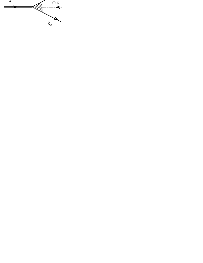
Figure 1: Graphical representation of the two-body wave function.

The wave function ${\mit\Phi}_{\sigma_{2}\sigma_{1}}$ of a two-fermion bound state is shown graphically in figure 1. It depends on four four-momenta

$${\mit\Phi}_{\sigma_{2}\sigma_{1}}={\mit\Phi}_{\sigma_{2}\sigma_{1}}(k_{1},k_{2},p,\omega\tau)$$ (1)

which are all on the corresponding mass shells ($k_{1}^{2}=k_{2}^{2}=m^{2}$, $p^{2}=M^{2}$, $(\omega\tau)^{2}=0$) and satisfy the conservation law:

$$k_{1}+k_{2}=p+\omega\tau.$$ (2)

In the standard approach the $+$ and $\perp$ components are conserved, whereas the minus-component is not. These properties are reproduced by equation (2), since in this case the only nonzero component is $\omega_{-}=2$. Equation (2) is thus a covariant generalization of the usual conservation law.

The general form of the wave function (1) depends on the particular quantum number of the state and is obtained by constructing all possible spin structures.

It is convenient to introduce variables ($\vec{k},\hat{n}$), constructed from the initial four-momenta as follows:

$$\vec{k} = L^{-1}({\cal P})\vec{k}_{1}=\vec{k}_{1}-\frac{\vec{\cal P}}{\sqrt{{\cal P}^{2}}}[k_{10}-\frac{\vec{k}_{1}\makebox[2.27626pt]{$\cdot$}\vec{{\cal P}}}{\sqrt{{\cal P}^{2}}+{\cal P}_{0}}]$$

$$\hat{n} = {L^{-1}({\cal P})\vec{\omega}\over|L^{-1}({\cal P})\vec{\omega}|}$$ (3)

where ${\cal P}=p+\omega\tau$, and $L^{-1}({\cal P})$ is the Lorentz boost into the reference system where $\vec{\cal P}=0$. In these variables, the wave function (1) is represented as:

$${\mit\Phi}_{\sigma_{2}\sigma_{1}}={\mit\Phi}_{\sigma_{2}\sigma_{1}}(\vec{k},\hat{n}).$$ (4)

Under Lorentz transformations of the four-momenta $k_{1},k_{2},p,\omega\tau$ the variables $\vec{k},\vec{n}$ are only rotated cdkm , so that parametrization (4), though being three-dimensional, is also explicitly covariant. In practice, instead of dealing with transformations (3), it is enough to write the wave functions and dynamical equations in the center of mass reference system, i.e. the one for which $\vec{\cal P}=\vec{k}_{1}+\vec{k}_{2}=0$ and in which $\vec{k}_{1}\equiv\vec{k}$, $\vec{k}_{2}\equiv-\vec{k}$, $\vec{\omega}\equiv\hat{n}|\vec{\omega}|$.

The equation for the wave function in terms of variables (3) reads:

$$\left[M^{2}-4(\vec{k}\,^{2}+m^{2})\right]{\mit\Phi}_{\sigma_{2}\sigma_{1}}(\vec{k},\vec{n})=\frac{m^{2}}{2\pi^{3}}\int\sum_{\sigma^{\prime}_{1}\sigma^{\prime}_{2}}K_{\sigma_{2}\sigma_{1}}^{\sigma^{\prime}_{2}\sigma^{\prime}_{1}}(\vec{k},\vec{k}\,^{\prime},\hat{n},M^{2}){\mit\Phi}_{\sigma^{\prime}_{2}\sigma^{\prime}_{1}}(\vec{k}\,^{\prime},\hat{n})\frac{d^{3}k^{\prime}}{\varepsilon_{k^{\prime}}}$$ (5)

where $K(\vec{k},\vec{k}\,^{\prime},\hat{n},M^{2})$ is the interaction kernel. It depends on the scalar products of the vectors $\vec{k}\,^{\prime},\vec{k},\vec{n}$ and also on the scalar products $\vec{k}\makebox[2.27626pt]{$\cdot$}\vec{\sigma}$, $\vec{k}\,^{\prime}\makebox[2.27626pt]{$\cdot$}\vec{\sigma}$ and $\hat{n}\makebox[2.27626pt]{$\cdot$}\vec{\sigma}$. For the Yukawa model it will be precised in next section.

In CLFD, the construction of states with definite angular momentum has some peculiarities which are explained in cdkm ; fermions . These peculiarities are related to the fact that the angular momentum operator $\vec{J}$ is not kinematical, but contains the interaction. However, we can overcome this difficulty by taking into account the so-called angular condition, derived from the transformation properties of the wave function under rotations of the light-front plane. Assuming that the state vector satisfies this condition, the problem results in finding the eigenfunctions of a purely kinematical operator $\vec{M}$

$$\vec{M}=-i\;\vec{k}\times{\partial\over\partial\vec{k}}\,-i\;\vec{n}\times{\partial\over\partial\vec{n}}+\vec{s}_{1}+\vec{s}_{2}\$$ (6)

where $\vec{s}_{i}$ are the fermion spin operators. The operators ($\vec{M}^{2}$, $M_{z}$) have the same eigenvalues $J(J+1)$ and $\lambda$ than the full angular momentum operators ($\vec{J}\,^{2}$, $J_{z}$).

As already mentioned, in any Lorentz transformation of the state vector, $\vec{k}$ and $\hat{n}$ undergo only rotations, with the same rotation operator than the one acting on spinor indices $\sigma_{1},\sigma_{2}$. In this respect, the eigenstates of $\vec{M}^{2},M_{z}$ are constructed as in the non relativistic quantum mechanics. The only difference is that we have at our disposal two three-dimensional vectors ($\vec{k},\hat{n}$) which enter in this construction on equal ground, instead of the only relative momentum $\vec{k}$ in the non relativistic case.

Since the interaction kernel in (5) depends on the scalar products of all the three-vectors, including spin operator, $\vec{M}$ commutes with it. The solutions of the equation (5) are eigenfunctions of the operators $\vec{M}^{2},M_{z}$ with eigenvalues $J(J+1)$ and $\lambda$.

Although the operator $\vec{M}$ contains the derivatives both over $\partial/\partial\vec{k}$ and $\partial/\partial\hat{n}$, its projection on $\hat{n}$-axis does not involve any derivative with respect to variable $\hat{n}$. Furthermore this latter enters in equation (5) as a vector parameter only and not as a dynamical variable. Therefore, there exists another operator which commutes with the kernel, namely:

$$A^{2}=(\hat{n}\makebox[2.27626pt]{$\cdot$}\vec{M})^{2}.$$ (7)

Since $A^{2}$ is a scalar, it commutes also with $\vec{M}$. Therefore, in addition to $J,J_{z}$, the solutions are labeled by $a$:

$$A^{2}\vec{\psi}^{a}(\vec{k},\hat{n})=a^{2}\vec{\psi}^{a}(\vec{k},\hat{n}).$$ (8)

The operator $A^{2}$ has $J+1$ eigenvalues, $a^{2}=0,1,\ldots,J^{2}$, and $2J+1$ eigenfunctions which are split in two families of $J$ and $J+1$ states with opposite parities. For $J=0$, there is only one value $a=0$. For $J^{\pi}=1^{+}$, there are two values $a=0$ and $a=1$. The wave function with definite $J$ is determined by $N_{J}={1\over 2}(2J+1)\times 2\times 2=2(2J+1)$ spin components (the ${1\over 2}$ factor comes from parity conservation). The system of equations for these $2(2J+1)$ spin components is split in different subsystems each of them with definite value of $a$. For example, the wave function for $J=1$ is determined by $N_{J}=6$ components ckj1 and the equation system is split in two subsystems corresponding to $a=0$ and $a=1$ and containing respectively 2 and 4 equations (see section IV).

The calculation technique of the CLFD is given by special graph rules which are a covariant generalization of the old fashioned perturbation theory. It was developed by Kadyshevsky kadysh and adapted to CLFD in karm76 ; cdkm . The equation for the wave function is shown graphically in figure 2 and the corresponding analytical form (5) is obtained by applying the rules of the graph techniques to the diagram displayed in this figure.

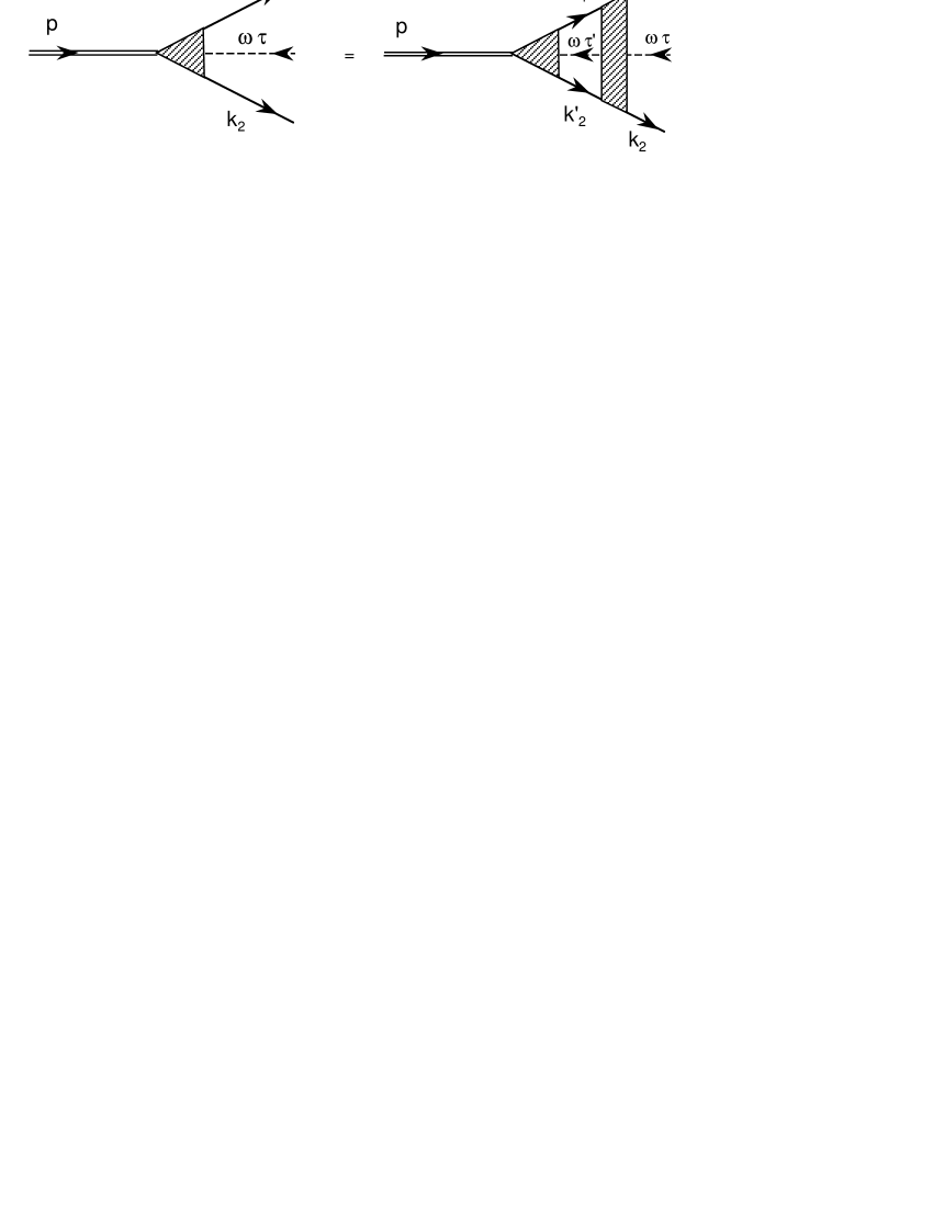
Figure 2: Equation for the two-body wave function.

All along this paper we will consider the one boson exchange kernel with scalar coupling only. The interaction Lagrangian is ${\cal L}^{int}=g\;\bar{\psi}\psi\phi^{(s)}$.

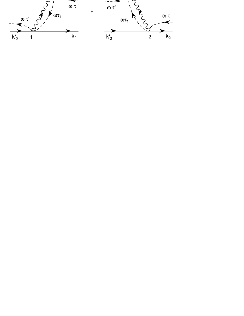
Figure 3: One boson exchange kernel.

The corresponding amplitude – represented graphically in figure 3 has the form:

$$K^{\sigma^{\prime}_{2}\sigma^{\prime}_{1}}_{\sigma_{2}\sigma_{1}} = -\frac{g^{2}}{4m^{2}}\left[\bar{u}^{\sigma_{2}}(k_{2})u^{\sigma^{\prime}_{2}}(k^{\prime}_{2})\right]\;\left[\bar{u}^{\sigma_{1}}(k_{1})u^{\sigma^{\prime}_{1}}(k^{\prime}_{1})\right]$$

$$\times\left\{\frac{\theta\left(\omega\makebox[2.27626pt]{$\cdot$}(k^{\prime}_{1}-k_{1})\right)}{\mu^{2}-(k^{\prime}_{1}-k_{1})^{2}+2\tau^{\prime}\omega\makebox[2.27626pt]{$\cdot$}(k^{\prime}_{1}-k_{1})}\right.+\left.\frac{\theta\left(\omega\makebox[2.27626pt]{$\cdot$}(k_{1}-k^{\prime}_{1})\right)}{\mu^{2}-(k_{1}-k^{\prime}_{1})^{2}+2\tau\omega\makebox[2.27626pt]{$\cdot$}(k_{1}-k^{\prime}_{1})}\right\}.$$

Like the wave function, the kernel is off energy shell for $\tau,\tau^{\prime}\neq 0$. The two terms can be simplified into:

$$K(k_{1},k_{2},\omega\tau;k^{\prime}_{1},k^{\prime}_{2},\omega\tau^{\prime})=-\frac{g^{2}}{4m^{2}(Q^{2}+\mu^{2})}\left[\bar{u}_{\sigma_{2}}(k_{2})u_{\sigma^{\prime}_{2}}(k^{\prime}_{2})\right]\,\left[\bar{u}_{\sigma_{1}}(k_{1})u_{\sigma^{\prime}_{1}}(k^{\prime}_{1})\right],$$ (10)

$Q^{2}$ is given in variables $\vec{k},\hat{n}$ by

$$Q^{2} = k^{2}+k^{\prime 2}-2kk^{\prime}\left(1+\frac{(\varepsilon_{k}-\varepsilon_{k^{\prime}})^{2}}{2\varepsilon_{k}\varepsilon_{k^{\prime}}}\right)\cos\theta\cos\theta^{\prime}-2kk^{\prime}\sin\theta\sin\theta^{\prime}\cos\varphi^{\prime}$$ (11)

$$+\left(\varepsilon_{k}^{2}+\varepsilon_{k^{\prime}}^{2}-\frac{1}{2}M^{2}\right)\left|\frac{k\cos\theta}{\varepsilon_{k}}-\frac{k^{\prime}\cos\theta^{\prime}}{\varepsilon_{k^{\prime}}}\right|$$

where $k\cos\theta=\hat{n}\makebox[2.27626pt]{$\cdot$}\vec{k}$, $k^{\prime}\cos\theta^{\prime}=\hat{n}\makebox[2.27626pt]{$\cdot$}\vec{k}^{\prime}$ and $\varphi^{\prime}$ is the azimuthal angle between $\vec{k}$ and $\vec{k}\,^{\prime}$ in the plane orthogonal to $\hat{n}$.

III The $J=0^{+}$ state

The wave function of a two fermion system in the state $J=0^{+}$ has the form ckj0 :

$${\mit\Phi}_{\sigma_{2}\sigma_{1}}(k_{1},k_{2},p,\omega\tau)=\sqrt{m}\overline{u}_{\sigma_{2}}(k_{2})\phi U_{c}\overline{u}_{\sigma_{1}}(k_{1}),$$ (12)

with

$$\phi=f_{1}S_{1}+f_{2}S_{2},$$ (13)

$f_{i}$ are scalar functions depending on $(k,\theta)$ and $S_{i}$ are spin structures given by

$$S_{1}=\frac{1}{2\sqrt{2}\varepsilon_{k}}\gamma_{5},\quad S_{2}=\frac{\varepsilon_{k}}{2\sqrt{2}mk\sin\theta}\left(\frac{2m\hat{\omega}}{\omega\makebox[2.27626pt]{$\cdot$}p}-\frac{m^{2}}{\varepsilon_{k}^{2}}\right)\gamma_{5}$$ (14)

in which $\hat{\omega}=\omega_{\mu}\gamma^{\mu}$ and $\varepsilon_{k}=\sqrt{k^{2}+m^{2}}$. $U_{c}=\gamma^{2}\gamma^{0}$ is the charge conjugation matrix, $u$ the usual spinor normalized as $\bar{u}_{\sigma}u_{\sigma^{\prime}}=2m\delta_{\sigma\sigma^{\prime}}$:

$$u_{\sigma}(k)=\sqrt{\varepsilon_{k}+m}\left(\begin{array}[]{c}1\\ \frac{\displaystyle\vec{\sigma}\makebox[2.27626pt]{$\cdot$}\vec{k}}{\displaystyle(\varepsilon_{k}+m)}\end{array}\right)w_{\sigma},$$ (15)

and $w_{\sigma}$ the two-component spinor normalized to $w^{\dagger}_{\sigma}w_{\sigma^{\prime}}=\delta_{\sigma\sigma^{\prime}}$.

Because of the spin structure $\hat{\omega}$, the relativistic wave function (12) is determined by two scalar functions, in the agreement with the counting rule mentioned above. In section V we will show that this state corresponds in the standard approach to the $(1+,2-)$ state discussed in glazek1 and described by the two components $\Phi^{1+},\Phi^{2-}$.

In the reference system where $\vec{k}_{1}+\vec{k}_{2}=0$, the wave function (12) can be represented as follows:

$${\mit\Phi}_{\sigma_{2}\sigma_{1}}=\sqrt{m}w_{\sigma_{2}}^{\dagger}\psi(\vec{k},\vec{n})w_{\sigma_{1}}^{\dagger}$$

with

$$\psi(\vec{k},\hat{n})=\frac{1}{\sqrt{2}}\left(f_{1}+\frac{i\vec{\sigma}\makebox[2.27626pt]{$\cdot$}[\vec{k}\times\hat{n}]}{k\sin\theta}f_{2}\right)\sigma_{y}$$ (16)

The normalization condition has the form:

$$\sum_{\sigma_{2}\sigma_{1}}\left|{\mit\Phi}_{\sigma_{2}\sigma_{1}}\right|^{2}={m\over(2\pi)^{3}}\int Tr\{\bar{\phi}(\hat{k}_{2}+m)\phi(\hat{k}_{1}-m)\}{d^{3}k\over\varepsilon_{k}}$$

$$={m\over(2\pi)^{3}}\int Tr\{\psi^{{\dagger}}(\vec{k},\vec{n})\psi(\vec{k},\vec{n})\}{d^{3}k\over\varepsilon_{k}}={m\over(2\pi)^{3}}\int(f_{1}^{2}+f_{2}^{2}){d^{3}k\over\varepsilon_{k}}=1,$$ (17)

where we denote $\hat{k}_{i}=k^{\mu}_{i}\gamma_{\mu}$ and $\bar{\phi}=\gamma_{0}\phi^{\dagger}\gamma_{0}$.

The spin structures $S_{i}$ in (14) are constructed in order to reproduce equation (16) without any additional coefficient and they are orthonormalized relative to the trace operation in (III):

$$Tr\{\bar{S}_{i}(\hat{k}_{2}+m)S_{j}(\hat{k}_{1}-m)\}=\delta_{ij},$$ (18)

where $\bar{S}_{i}=\gamma_{0}S_{i}^{\dagger}\gamma_{0}$, that is:

$$\bar{S}_{1}=-\frac{1}{2\sqrt{2}\varepsilon_{k}}\gamma_{5},\quad\bar{S}_{2}=-\frac{\varepsilon_{k}}{2\sqrt{2}mk\sin\theta}\gamma_{5}\left(\frac{2m\hat{\omega}}{\omega\makebox[2.27626pt]{$\cdot$}p}-\frac{m^{2}}{\varepsilon_{k}^{2}}\right).$$ (19)

We insert expression (12) for the wave function in equation (5) and multiply it on left by $u(k_{2})$ and on right by $u(k_{1})$. Using the relation $\sum_{\sigma}u^{\sigma}(k)\bar{u}^{\sigma}(k)=\hat{k}+m$, we get:

$$\left[M^{2}-4(\vec{k}\,^{2}+m^{2})\right](\hat{k}_{2}+m)\phi(\hat{k}_{1}-m)$$ (20)

$$=\frac{m^{2}}{2\pi^{3}}\int\frac{g^{2}}{4m^{2}(Q^{2}+\mu^{2})}(\hat{k}_{2}+m)(\hat{k}^{\prime}_{2}+m)\phi^{\prime}(\hat{k}^{\prime}_{1}-m)(\hat{k}_{1}-m)\frac{d^{3}k^{\prime}}{\varepsilon_{k^{\prime}}}.$$

Substituting $\phi$ in the form (13), multiplying equation (20) by $\bar{S}_{i}$ from (19) and using the orthogonality relation (18), we obtain the system of two-dimensional integral equations for the components $f_{i}$:

$$\left[M^{2}-4(\vec{k}\,^{2}+m^{2})\right]f_{1}(k,\theta) = \frac{m^{2}}{2\pi^{3}}\int\left[K_{11}(k,\theta;k^{\prime},\theta^{\prime})f_{1}(k^{\prime},\theta^{\prime})+K_{12}(k,\theta;k^{\prime},\theta^{\prime})f_{2}(k^{\prime},\theta^{\prime})\right]\frac{d^{3}k^{\prime}}{\varepsilon_{k^{\prime}}}$$

$$\left[M^{2}-4(\vec{k}\,^{2}+m^{2})\right]f_{2}(k,\theta) = \frac{m^{2}}{2\pi^{3}}\int\left[K_{21}(k,\theta;k^{\prime},\theta^{\prime})f_{1}(k^{\prime},\theta^{\prime})+K_{22}(k,\theta;k^{\prime},\theta^{\prime})f_{2}(k^{\prime},\theta^{\prime})\right]\frac{d^{3}k^{\prime}}{\varepsilon_{k^{\prime}}}$$ (21)

The kernels $K_{ij}$ result from a first integration over the azimuthal angle $\varphi^{\prime}$ of more elementary quantities:

$$K_{ij} = {1\over m^{2}\varepsilon_{k}\varepsilon_{k^{\prime}}}\int_{0}^{2\pi}{\kappa_{ij}\over Q^{2}+\mu^{2}}{d\varphi^{\prime}\over 2\pi}$$ (22)

with

$$\kappa_{ij} = {g^{2}\over 4}\varepsilon_{k}\varepsilon_{k}^{\prime}Tr\left[\bar{S}_{i}(\hat{k}_{2}+m)(\hat{k^{\prime}}_{2}+m)S^{\prime}_{j}(\hat{k^{\prime}}_{1}-m)(\hat{k}_{1}-m)\right]$$ (23)

However, for notation convenience, we keep in (III) the three dimensional volume element though the kernels (22) are $\varphi^{\prime}$ independent. The traces (23) are expressed through the scalar products of the available four-vectors. The analytical expressions for these scalar products and for $\kappa_{ij}$ in the variables $k,k^{\prime},\theta,\theta^{\prime},\varphi^{\prime}$ are given in appendix A.

IV The $J=1^{+}$ state

As mentioned in section II, the two-fermion wave function with $J=1^{+}$ is determined by six components associated to each of the six spin structures one can construct karm81 :

$$S_{1\mu}=\frac{(k_{1}-k_{2})^{\mu}}{2m^{2}},\quad S_{2\mu}=\frac{1}{m}\gamma^{\mu},\quad S_{3\mu}=\frac{\omega^{\mu}}{\omega\makebox[2.27626pt]{$\cdot$}p},\quad S_{4\mu}=\frac{(k_{1}-k_{2})^{\mu}\hat{\omega}}{2m\omega\makebox[2.27626pt]{$\cdot$}p},$$

$$S_{5\mu}=-\frac{i}{m^{2}\omega\makebox[2.27626pt]{$\cdot$}p}\gamma_{5}\epsilon^{\mu\nu\rho\gamma}k_{1\nu}k_{2\rho}\omega_{\gamma},\quad S_{6\mu}=\frac{m\omega^{\mu}\hat{\omega}}{(\omega\makebox[2.27626pt]{$\cdot$}p)^{2}}.$$ (24)

The system of equations satisfying by these components can be split in two subsystems corresponding respectively to the eigenvalues $a=0,1$ of the operator $A^{2}$ (7). The subsystem $a=0$ is – like in the $J=0$ case – determined by two components whereas the four remaining components are related to $a=1$. The total number of components as well as the dimensions of the subsystems (2+4) coincides with the results obtained in the standard approach glazek1 .

IV.1 The case $a=0$

In this section we consider the state with $a=0$. We represent the wave function in a form similar to (12)

$${\mit\Phi}^{\lambda}_{\sigma_{2}\sigma_{1}}(k_{1},k_{2},p,\omega\tau)=\sqrt{m}e^{\mu}(p,\lambda)\bar{u}^{\sigma_{2}}(k_{2})\phi^{(0)}_{\mu}U_{c}\bar{u}^{\sigma_{1}}(k_{1})\ ,$$ (25)

$e^{\mu}(p,\lambda)$ is the spin-1 polarization vector and functions $\phi^{(0)}_{\mu}$ are represented as:

$$\phi^{(0)}_{\mu}=g^{(0)}_{1}S^{(0)}_{1\mu}+g^{(0)}_{2}S^{(0)}_{2\mu}.$$ (26)

where $g^{(0)}_{i}$ are scalar functions and the spin structures $S^{(0)}_{i\mu}$ will be expressed in terms of structures (IV).

In the reference system where $\vec{k}_{1}+\vec{k}_{2}=0$ this wave function can be represented in the form:

$${\mit\Phi}^{\lambda}_{\sigma_{2}\sigma_{1}}(\vec{k},\hat{n})=\sqrt{m}w^{\dagger}_{\sigma_{2}}\psi^{(0)}_{\lambda}(\vec{k},\hat{n})\sigma_{y}w^{\dagger}_{\sigma_{1}}.$$ (27)

One can easily check that the function $\vec{\psi}^{0}(\vec{k},\hat{n})$ – satisfying equation (8) with $a=0$ – is proportional to $\hat{n}$, i.e. it satisfies the condition $\vec{\psi}^{0}=\hat{n}(\hat{n}\makebox[2.27626pt]{$\cdot$}\vec{\psi}^{0})$. Since we are dealing with a $J^{\pi}=1^{+}$ pseudovector state, it has the following general decomposition:

$$\vec{\psi}^{0}(\vec{k},\vec{n})=\sqrt{\frac{3}{2}}\left\{g^{(0)}_{1}\vec{\sigma}\makebox[2.27626pt]{$\cdot$}\hat{k}+g^{(0)}_{2}\frac{\vec{\sigma}\makebox[2.27626pt]{$\cdot$}(\hat{k}\cos\theta-\hat{n})}{\sin\theta}\right\}\hat{n}$$ (28)

in which the vector $\hat{n}$ is multiplied by the two only pseudoscalar structures one can construct $\vec{\sigma}\makebox[2.27626pt]{$\cdot$}\vec{k}$ and $\vec{\sigma}\makebox[2.27626pt]{$\cdot$}\hat{n}$.

The four-dimensional structures $S^{(0)}_{1,2\mu}$ are built in terms of $S_{i\mu}$ defined in (IV) in a way to obtain equation (28) from (25) written in the c.m.-system. One finds

$$S^{(0)}_{1\mu}=\frac{\sqrt{3}M}{2\sqrt{2}k}S_{3\mu}\qquad S^{(0)}_{2\mu}=\frac{\sqrt{3}M}{m\sqrt{2}\sin\theta}\left(\frac{m^{2}\cos\theta}{2\varepsilon_{k}k}S_{3\mu}+S_{6\mu}\right),$$ (29)

The normalization condition for the wave function reads:

$$\frac{1}{3}\sum_{\lambda\sigma_{2}\sigma_{1}}\left|{\mit\Phi}^{\lambda}_{\sigma_{2}\sigma_{1}}\right|^{2}={m\over(2\pi)^{3}}\int\Pi^{\mu\nu}Tr\{\phi^{(0)}_{\mu}(\hat{k}_{2}+m)\phi^{(0)}_{\nu}(\hat{k}_{1}-m)\}{d^{3}k\over\varepsilon_{k}}$$

$$= {m\over 3(2\pi)^{3}}\int Tr\{\vec{\psi}^{(0){\dagger}}(\vec{k},\vec{n})\vec{\psi}^{(0)}(\vec{k},\vec{n})\}{d^{3}k\over\varepsilon_{k}}={m\over(2\pi)^{3}}\int\left[(g^{(0)}_{1})^{2}+(g^{(0)}_{2})^{2}\right]{d^{3}k\over\varepsilon_{k}}=1.$$

where we have introduced the tensor

$$\Pi^{\mu\nu}=\frac{1}{3}\sum_{\lambda}e^{\mu*}(p,\lambda)e^{\nu}(p,\lambda)=\frac{1}{3}\left(\frac{p^{\mu}p^{\nu}}{M^{2}}-g^{\mu\nu}\right).$$ (31)

The structures $S^{(0)}_{i}$ are orthonormalized relative to the trace operation:

$$\Pi^{\mu\nu}Tr\{\bar{S}^{(0)}_{i\mu}(\hat{k}_{2}+m)S^{(0)}_{j\nu}(\hat{k}_{1}-m)\}=\delta_{ij}$$ (32)

with $\bar{S}^{(0)}_{i\mu}=\gamma_{0}S^{(0)\dagger}_{i\mu}\gamma_{0}=S^{(0)}_{i\mu}$. The same relation and the orthogonality condition (32) hold for the structures $S^{(1)}_{i\mu}$ corresponding to $a=1$ and constructed in the next section.

We finally obtain for the components $g^{(0)}_{i}$ a system of two equations having the same form than for J=0 – (III) and (22) – with kernels $\kappa_{ij}$ given by:

$$\kappa_{ij}={g^{2}\over 4}\varepsilon_{k}\varepsilon_{k}^{\prime}\Pi^{\mu\nu}Tr\left[\bar{S}^{(0)}_{i\mu}(\hat{k}_{2}+m)(\hat{k^{\prime}}_{2}+m)S^{\prime(0)}_{j\nu}(\hat{k^{\prime}}_{1}-m)(\hat{k}_{1}-m)\right].$$ (33)

Their explicit analytical expressions are given in appendix A.

IV.2 The case $a=1$

The solution $\vec{\psi}^{1}(\vec{k},\hat{n})$ corresponding to $a=1$ is orthogonal to $\hat{n}$, i.e. it satisfies $\hat{n}\makebox[2.27626pt]{$\cdot$}\vec{\psi}^{1}=0$. To fulfill this condition, it is convenient to introduce the vectors $\hat{k}_{\perp}$ and $\vec{\sigma}_{\perp}$ orthogonal to $\hat{n}$:

$$\hat{k}_{\perp}=\frac{\vec{k}-k\cos\theta\hat{n}}{k\sin\theta}\qquad\vec{\sigma}_{\perp}=\vec{\sigma}-(\hat{n}\makebox[2.27626pt]{$\cdot$}\vec{\sigma})\hat{n}$$

and to write down $\vec{\psi}^{1}$ in the form:

$$\vec{\psi}^{1}(\vec{k},\vec{n})=\frac{\sqrt{3}}{2}\left\{g^{(1)}_{1}\vec{\sigma}_{\perp}+g^{(1)}_{2}\left(2\hat{\vec{k}}_{\perp}(\hat{\vec{k}}_{\perp}\makebox[2.27626pt]{$\cdot$}\vec{\sigma}_{\perp})-\vec{\sigma}_{\perp}\right)+g^{(1)}_{3}\hat{\vec{k}}_{\perp}(\vec{\sigma}\makebox[2.27626pt]{$\cdot$}\vec{n})+g^{(1)}_{4}i[\hat{\vec{k}}\times\vec{n}]\right\}$$ (34)

The four-dimensional representation ${\mit\Phi}^{\lambda}_{\sigma_{2}\sigma_{1}}$ analogous to (25), is written in terms of $\phi^{(1)}_{\mu}$:

$$\phi^{(1)}_{\mu}=g^{(1)}_{1}S^{(1)}_{1\mu}+g^{(1)}_{2}S^{(1)}_{2\mu}+g^{(1)}_{3}S^{(1)}_{3\mu}+g^{(1)}_{4}S^{(1)}_{4\mu}.$$ (35)

The four spin structures $S^{(1)}_{j\mu}$ are orthonormalized according to (32) and read:

$$S^{(1)}_{i\mu}=\sum_{j}\eta_{ij}S_{j\mu},\quad i=1,\ldots,4;\;j=1,\ldots,6,$$ (36)

with $S_{j\mu}$ defined in (IV) and the coefficients $\eta_{ij}$ given in appendix B.

The normalization condition in terms of $\phi^{(1)}_{\mu}$ and $\vec{\psi}^{(1)}$ exactly coincides with (IV.1) and in terms of the components $g^{(1)}_{i}$ is rewritten as:

$${m\over(2\pi)^{3}}\int\left[(g^{(1)}_{1})^{2}+(g^{(1)}_{2})^{2}+(g^{(1)}_{3})^{2}+(g^{(1)}_{4})^{2}\right]{d^{3}k\over\varepsilon_{k}}=1.$$ (37)

The system of equations for the four scalar functions $g^{(1)}_{i}$ has also the same form than (III)

$$\left[M^{2}-4(\vec{k}\,^{2}+m^{2})\right]g^{(1)}_{i}(\vec{k},\hat{n})=\frac{m^{2}}{2\pi^{3}}\int\sum_{j=1}^{4}K^{(1)}_{ij}(\vec{k},\vec{k}\,^{\prime},\hat{n})g^{(1)}_{j}(\vec{k}\,^{\prime},\hat{n})\frac{d^{3}k^{\prime}}{\varepsilon_{k^{\prime}}}$$ (38)

The kernels $K^{(1)}_{ij}$ are obtained from (33) by substituting $S^{(1)}$ instead of $S^{(0)}$. Their analytical expressions are given in appendix A. The details of calculation can be found in These_MMB .

We are interested here in calculating the mass $M$ of a J=1 state. The physical solution satisfying the angular condition mentioned above is given by the superposition of the solutions ($\psi_{a},M_{a}$) with definite $a$ fermions ; heidelberg :

$$\vec{\psi}=c_{0}\vec{\psi}^{0}+c_{1}\vec{\psi}^{1}.$$

The corresponding mass is

$$M^{2}=c_{0}^{2}M_{0}^{2}+c_{1}^{2}M_{1}^{2}$$

V Relation with the standard approach

In reference glazek1 , the system of equations solved for the $J_{z}=0$ helicity sector had the form:

$$\left(M^{2}-M_{0}^{2}\right)\Phi_{1}(R_{\perp},x)$$

$$=\frac{\alpha}{4\pi^{2}}\int\left[V_{11}(R_{\perp},x;R_{\perp}^{\prime},x^{\prime})\Phi_{1}(R_{\perp}^{\prime},x^{\prime})+V_{12}(R_{\perp},x;R_{\perp}^{\prime},x^{\prime})\Phi_{2}(R_{\perp}^{\prime},x^{\prime})\right]R_{\perp}^{\prime}dR_{\perp}^{\prime}dx^{\prime},$$

$$\left(M^{2}-M_{0}^{2}\right)\Phi_{2}(R_{\perp},x)$$ (39)

$$=\frac{\alpha}{4\pi^{2}}\int\left[V_{21}(R_{\perp},x;R_{\perp}^{\prime},x^{\prime})\Phi_{1}(R_{\perp}^{\prime},x^{\prime})+V_{22}(R_{\perp},x;R_{\perp}^{\prime},x^{\prime})\Phi_{2}(R_{\perp}^{\prime},x^{\prime})\right]R_{\perp}^{\prime}dR_{\perp}^{\prime}dx^{\prime},$$

with $M_{0}^{2}={R_{\perp}^{2}+m^{2}\over x(1-x)}$. They correspond to equations (3.1a), (3.1b) from glazek1 with the notations $k\equiv R_{\perp}$, $q\equiv R^{\prime}_{\perp}$, $y\equiv x^{\prime}$. The coupled wave functions ($\Phi_{1},\Phi_{2}$) should be identified either to ($\Phi^{1+},\Phi^{2-}$) or to ($\Phi^{1-},\Phi^{2+}$) sets. The kernels $V_{ij}$, given by eqs. C1-C4 in glazek1 , are for the case ($\Phi^{1+},\Phi^{2-}$):

$$V_{ij} = \int_{0}^{2\pi}\frac{v_{ij}d\varphi^{\prime}}{x(1-x)x^{\prime}(1-x^{\prime})(Q^{2}+\mu^{2})},$$

$$v_{11} = R_{\perp}R_{\perp}^{\prime}(2xx^{\prime}-x-x^{\prime})$$

$$+\left[R_{\perp}^{2}x^{\prime}(1-x^{\prime})+R^{\prime 2}_{\perp}x(1-x)-m^{2}(x+x^{\prime})(2-x-x^{\prime})\right]\cos\varphi^{\prime},$$

$$v_{12} = m\left[R_{\perp}(x+3x^{\prime}-2xx^{\prime}-2x^{\prime 2})-R^{\prime}_{\perp}(x^{\prime}+3x-2x^{\prime}x-2x^{2})\cos\varphi^{\prime}\right],$$

$$v_{21} = m\left[R^{\prime}_{\perp}(x^{\prime}+3x-2x^{\prime}x-2x^{2})-R_{\perp}(x+3x^{\prime}-2xx^{\prime}-2x^{\prime 2})\cos\varphi^{\prime}\right],$$

$$v_{22} = R_{\perp}R_{\perp}^{\prime}(2xx^{\prime}-x-x^{\prime})\cos\varphi^{\prime}$$

$$+\left[R_{\perp}^{2}x^{\prime}(1-x^{\prime})+R^{\prime 2}_{\perp}x(1-x)-m^{2}(x+x^{\prime})(2-x-x^{\prime})\right].$$

The momentum transfer $Q^{2}$ reads:

$$Q^{2}=m^{2}{x^{\prime}\over x}\left(1-\frac{x}{x^{\prime}}\right)^{2}+\frac{x^{\prime}}{x}R_{\perp}^{2}-2R_{\perp}R_{\perp}^{\prime}\cos\varphi^{\prime}+\frac{x}{x^{\prime}}R_{\perp}^{\prime 2}+(x^{\prime}-x)\left(\frac{m^{2}+R_{\perp}^{\prime 2}}{x^{\prime}(1-x^{\prime})}-M^{2}\right)$$ (41)

for $x\leq x^{\prime}$ and with the replacements $x\leftrightarrow x^{\prime}$ $R_{\perp}\leftrightarrow R_{\perp}^{\prime}$ for $x\geq x^{\prime}$.

The functions $\Phi_{i}$ are normalized as:

$$\int\left(|\Phi_{1}(R_{\perp},x)|^{2}+|\Phi_{2}(R_{\perp},x)|^{2}\right)R_{\perp}\,dR_{\perp}\,dx=1.$$ (42)

We will show that the equations (III) with kernels (A) corresponding to our $J=0$ state are identical to equations (V) with kernels (V) for ($\Phi^{1+},\Phi^{2-}$). They transform into each other by a linear combination of the wave functions and by a change of variable. The relation between the wave functions can be written in the form:

$$f_{j}=N(x)\sum_{i}\Phi_{i}\;c_{ij}(R_{\perp})$$ (43)

with a normalization factor ensuring the equivalence between the conditions (III) and (42)

$$N(x)=2^{3/2}\pi m^{-1/2}\sqrt{x(1-x)}$$

and a unitary matrix $\hat{c}$:

$$\hat{c}={1\over\sqrt{R_{\perp}^{2}+m^{2}}}\pmatrix{-R_{\perp}&m\cr m&R_{\perp}}$$ (44)

Variables $(R_{\perp},x)$ used in (V) are related to $(k,\theta)$ from (III) by:

$$R_{\perp}=k\sin\theta,\qquad x=\frac{1}{2}\left(1-\frac{k\cos\theta}{\varepsilon_{k}}\right)$$ (45)

and their reversed relations:

$$k^{2}=\frac{R_{\perp}^{2}+m^{2}}{4x(1-x)}-m^{2},\quad\cos\theta=\frac{(1-2x)\sqrt{R_{\perp}^{2}+m^{2}}}{\sqrt{R_{\perp}^{2}+m^{2}(1-2x)^{2}}}.$$ (46)

Variables $(\vec{R}_{\perp},x)$ can be directly constructed from the initial four-momenta as follows. We introduce the four-vector $R=k_{1}-xp$ with $x=\omega\makebox[2.27626pt]{$\cdot$}k_{1}/(\omega\makebox[2.27626pt]{$\cdot$}p)$ and represent its spatial part as $\vec{R}=\vec{R}_{\|}+\vec{R_{\perp}}$, where $\vec{R}_{\|}$ is parallel to $\vec{\omega}$ and $\vec{R}_{\perp}\makebox[2.27626pt]{$\cdot$}\vec{\omega}=0$. Since by definition of $R$, $R\makebox[2.27626pt]{$\cdot$}\omega=R_{0}\omega_{0}-\vec{R}_{\|}\makebox[2.27626pt]{$\cdot$}\vec{\omega}=0$, it follows that $|R_{0}|=|\vec{R}_{\|}|$, and hence $\vec{R}^{2}_{\perp}=-R^{2}$ is invariant.

For $J=1,a=0$ quantum numbers, corresponding to the state $(1^{-},2^{+})$ from glazek1 , the relation between the $g^{(0)}_{j}$ components  and $\Phi_{i}$ is the same than (43)

$$g^{(0)}_{j}=N(x)\sum_{i}c_{ij}(R_{\perp})\Phi_{i}$$ (47)

with a $\hat{c}$ matrix

$$\hat{c}={1\over k\sqrt{R_{\perp}^{2}+m^{2}}}\pmatrix{R_{\perp}\varepsilon_{k}&-k_{z}m\cr-k_{z}m&-R_{\perp}\varepsilon_{k}}$$ (48)

Note that in glazek1 $k_{z}=-k\cos\theta$ with a minus sign due to $\hat{n}=-\hat{z}$).

Inserting (43) into equations (III), we reproduce equations (V) with kernels $V_{ij}$ which are linear combinations of $K_{ij}$:

$$V_{ij}={N(x^{\prime})\over N(x)N_{1}(x^{\prime})}\sum_{i^{\prime}j^{\prime}}c_{i^{\prime}i}(R_{\perp})K_{i^{\prime}j^{\prime}}c_{j^{\prime}j}(R^{\prime}_{\perp}),\qquad N_{1}(x^{\prime})={\alpha\pi\over m^{2}}x^{\prime}(1-x^{\prime}).$$ (49)

Substituting here the kernels $K_{ij}$ from (22) for $J=0$, we get the expressions for $V_{ij}$ given by (V). A similar identity is obtained for the kernels $K_{ij}$ of $J=1,a=0$ state (A) and the kernels $V_{ij}$ for the corresponding ($1^{-},2^{+}$) state considered in glazek1 . Hence, both systems of equations are strictly equivalent.

It is useful to explain the origin of the linear transformations (43) and (47). They result from using different representations of the spinors and different normalizations of the wave functions. Namely, instead of eq. (15) the following spinor is defined in glazek1 :

$$u^{LF}_{\sigma}(k)=\sqrt{\frac{2}{k_{0}+k_{3}}}\left[m\Lambda^{-}+(k_{0}+k_{3}+\gamma_{0}\vec{\gamma}^{\perp}\makebox[2.27626pt]{$\cdot$}\vec{k}^{\perp})\Lambda^{+}\right]\left(\begin{array}[]{l}w_{\sigma}\\ 0\end{array}\right)$$ (50)

where

$$\Lambda^{\pm}=\frac{1}{4}\gamma^{\mp}\gamma^{\pm},\quad\gamma^{\pm}=\gamma_{0}\pm\gamma_{3},\quad\vec{k}^{\perp}=(k_{1},k_{2}).$$

It can be transformed to the form:

$$u^{LF}_{\sigma}(k)=\sqrt{\frac{1}{2(k_{0}+k_{3})}}\left(\begin{array}[]{l}m+k_{0}+\vec{\sigma}\makebox[2.27626pt]{$\cdot$}\vec{k}\,\sigma_{3}\\ (k_{0}-m)\,\sigma_{3}+\vec{\sigma}\makebox[2.27626pt]{$\cdot$}\vec{k}\end{array}\right)w_{\sigma}$$ (51)

In order to relate the two wave functions, one may express the spinors $u^{LF}$ in terms of $u$:

$$u^{LF}_{\sigma}(k)=\sum_{\sigma^{\prime}=\pm\frac{1}{2}}\beta_{\sigma\sigma^{\prime}}(k)u_{\sigma^{\prime}}(k).$$ (52)

With the explicit formulas (15) and (51) we find:

$$\beta_{\sigma\sigma^{\prime}}(k)=\frac{1}{2m}\bar{u}_{\sigma^{\prime}}(k)u^{LF}_{\sigma}(k)=\sqrt{\frac{k_{0}+m}{2(k_{0}+k_{3})}}w^{\dagger}_{\sigma^{\prime}}\left(1+\frac{\vec{\sigma}\makebox[2.27626pt]{$\cdot$}\vec{k}\,\sigma_{3}}{k_{0}+m}\right)w_{\sigma}$$ (53)

Note the opposite order of indices in both sides of (53). Below we give explicitly these matrix elements in the c.m.-system $\vec{k}_{1}+\vec{k}_{2}=0$:

$$\beta_{\frac{1}{2}\frac{1}{2}}(k_{1})=\beta_{-\frac{1}{2}-\frac{1}{2}}(k_{1})=\frac{(k^{+}+m)}{\sqrt{2k^{+}(k_{0}+m)}},\quad\beta_{\frac{1}{2}-\frac{1}{2}}(k_{1})=-\beta^{*}_{-\frac{1}{2}\frac{1}{2}}(k_{1})=\frac{k_{\perp}e^{i\phi}}{\sqrt{2k^{+}(k_{0}+m)}},$$

$$\beta_{\frac{1}{2}\frac{1}{2}}(k_{2})=\beta_{-\frac{1}{2}-\frac{1}{2}}(k_{2})=\frac{(k^{-}+m)}{\sqrt{2k^{-}(k_{0}+m)}},\quad\beta_{\frac{1}{2}-\frac{1}{2}}(k_{2})=-\beta^{*}_{-\frac{1}{2}\frac{1}{2}}(k_{2})=\frac{-k_{\perp}e^{i\phi}}{\sqrt{2k^{-}(k_{0}+m)}},$$

with $k_{1}+ik_{2}=k_{\perp}e^{i\phi}$. Coefficients $\beta(k_{1})$ relate the spinors of particle 1 with momentum $\vec{k}_{1}=\vec{k}$, whereas coefficients $\beta(k_{2})$ relate the spinors of particle 2 with momentum $\vec{k}_{2}=-\vec{k}$). For the conjugated spinors $\bar{u}$ we get:

$$\bar{u}^{LF}_{\sigma_{1}}(k_{1})=\sum_{\sigma^{\prime}_{1}=\pm\frac{1}{2}}\beta^{*}_{\sigma_{1}\sigma^{\prime}_{1}}(k_{1})\bar{u}_{\sigma^{\prime}_{1}}(k_{1}),\quad\bar{u}^{LF}_{\sigma_{2}}(k_{2})=\sum_{\sigma^{\prime}_{2}=\pm\frac{1}{2}}\beta^{*}_{\sigma_{2}\sigma^{\prime}_{2}}(k_{2})\bar{u}_{\sigma^{\prime}_{2}}(k_{2}),$$ (55)

The matrix $\beta$ is unitary: $\sum_{\sigma^{\prime}}\beta^{\dagger}_{\sigma\sigma^{\prime}}\beta_{\sigma^{\prime}\sigma^{\prime\prime}}=\sum_{\sigma^{\prime}}\beta^{*}_{\sigma^{\prime}\sigma}\beta_{\sigma^{\prime}\sigma^{\prime\prime}}=\delta_{\sigma\sigma^{\prime\prime}}$. Substituting the spinors (55) into the wave function $\Psi$ defined by means of the spinors $\bar{u}^{LF}$, we get the relation:

$$\Psi^{\sigma_{1}\sigma_{2}}=\sum_{\sigma^{\prime}_{1}\sigma^{\prime}_{2}}\beta^{*}_{\sigma_{1}\sigma^{\prime}_{1}}(k_{1})\beta^{*}_{\sigma_{2}\sigma^{\prime}_{2}}(k_{2})\psi_{\sigma^{\prime}_{2}\sigma^{\prime}_{1}}$$ (56)

Note the opposite order of indices at $\Psi^{\sigma_{1}\sigma_{2}}$ and $\psi_{\sigma^{\prime}_{2}\sigma^{\prime}_{1}}$, in accordance with the above definitions. The matrix elements of the wave function $\psi(\vec{k},\vec{n})$ for $J=0$, eq. (16), are the following:

$$\psi_{\frac{1}{2}\frac{1}{2}}=\psi^{*}_{-\frac{1}{2}-\frac{1}{2}}=\frac{i}{\sqrt{2}}f_{2}e^{-i\phi},\quad\psi_{\frac{1}{2}-\frac{1}{2}}=-\psi_{\frac{1}{2}-\frac{1}{2}}=-\frac{i}{\sqrt{2}}f_{1}.$$ (57)

We substitute in (56) the coefficients (V) and the wave function (57), following the paper glazek1 , separate the phase factor:

$$\Psi^{\sigma_{1}\sigma_{2}}(\vec{R}^{\perp},x)=\sum_{m}\frac{e^{im\phi}}{\sqrt{2\pi}}\Phi^{\sigma_{1}\sigma_{2}}(R,x,m)$$

and introduce the following linear combinations:

$$\Phi^{1\pm}(R,x) = \frac{1}{\sqrt{2}}[\Phi^{\frac{1}{2}\frac{1}{2}}(R,x;-1)\pm\Phi^{-\frac{1}{2}-\frac{1}{2}}(R,x;1)],$$

$$\Phi^{2\pm}(R,x) = \frac{1}{\sqrt{2}}[\Phi^{\frac{1}{2}-\frac{1}{2}}(R,x;0)\pm\Phi^{-\frac{1}{2}\frac{1}{2}}(R,x;0)]$$ (58)

normalized according to (42). In this way we reproduce for $\Phi^{1+},\Phi^{2-}$ the relation (43) with coefficients (44). For the other pair of components we get $\Phi^{1-}=\Phi^{2+}=0$.

Similarly, taking the matrix elements of the wave function $\vec{\psi}^{(0)}(\vec{k},\hat{n})$ for $J=1,a=0$, equation (28), projected on the direction $\hat{n}$ (we remind that in the standard approach $\hat{n}||-z$), we find:

$$\vec{n}\makebox[2.27626pt]{$\cdot$}\vec{\psi}^{(0)}_{\frac{1}{2}\frac{1}{2}}=\vec{n}\makebox[2.27626pt]{$\cdot$}\vec{\psi}^{(0)*}_{-\frac{1}{2}-\frac{1}{2}}=\frac{i}{\sqrt{2}k}(g^{(0)}_{1}R_{\perp}-g^{(0)}_{2}k_{3})e^{-i\phi},$$

$$\vec{n}\makebox[2.27626pt]{$\cdot$}\vec{\psi}^{(0)}_{\frac{1}{2}-\frac{1}{2}}=\vec{n}\makebox[2.27626pt]{$\cdot$}\vec{\psi}^{(0)}_{\frac{1}{2}-\frac{1}{2}}=-\frac{i}{\sqrt{2}k}(g^{(0)}_{1}k_{3}+g^{(0)}_{2}R_{\perp}).$$

In this way we reproduce for $(\Phi^{1-},\Phi^{2+})$ the relation (47) with coefficients (48), whereas we get $\Phi^{1+}=\Phi^{2-}=0.$

VI Asymptotical properties and critical coupling constant

The stability of solutions is determined by the asymptotical behavior of kernels $K_{ij}$. This can be considered either for a fixed $k(k^{\prime})$ in the limit $k^{\prime}(k)\rightarrow\infty$ or in the limit of both $k,k^{\prime}\rightarrow\infty$ with a fixed ratio $\gamma={k^{\prime}\over k}$. We illustrate in what follows the analyzing method for the $J=0$ state. The relevant results for $J=1$ are summarized at the end of the section.

For a fixed value of $k(k^{\prime})$ we get:

$$K_{11}(k,\theta,k^{\prime},\theta^{\prime})\sim\left\{\begin{array}[]{ll}\frac{c_{11}}{k}&\mbox{if $k\to\infty$, $k^{\prime}$ fixed}\\ &\\ \frac{c^{\prime}_{11}}{k^{\prime}}&\mbox{if $k^{\prime}\to\infty$, $k$ fixed}\end{array}\right.$$ (62)

$$K_{12}(k,\theta,k^{\prime},\theta^{\prime})\sim\left\{\begin{array}[]{ll}\frac{c_{12}}{k}&\mbox{if $k\to\infty$, $k^{\prime}$ fixed}\\ &\\ c^{\prime}_{12}&\mbox{if $k^{\prime}\to\infty$, $k$ fixed}\end{array}\right.$$ (66)

$$K_{21}(k,\theta,k^{\prime},\theta^{\prime})\sim\left\{\begin{array}[]{ll}c_{21}&\mbox{if $k\to\infty$, $k^{\prime}$ fixed}\\ &\\ \frac{c^{\prime}_{21}}{k^{\prime}}&\mbox{if $k^{\prime}\to\infty$, $k$ fixed}\end{array}\right.$$ (70)

$$K_{22}(k,\theta,k^{\prime},\theta^{\prime})\sim\left\{\begin{array}[]{ll}c_{22}&\mbox{if $k\to\infty$, $k^{\prime}$ fixed}\\ &\\ c^{\prime}_{22}&\mbox{if $k^{\prime}\to\infty$, $k$ fixed}\end{array}\right.$$ (74)

with coefficients $c_{11},c_{12},c_{21},c_{22}$ depending on $k^{\prime},\theta,\theta^{\prime}$ and $c^{\prime}_{11},c^{\prime}_{12},c^{\prime}_{21},c^{\prime}_{22}$ depending on $k,\theta,\theta^{\prime}$.

One has for instance

$$c_{22}=\frac{\alpha\pi k^{\prime}\sin\theta\sin\theta^{\prime}}{m^{2}(\varepsilon_{k^{\prime}}-k^{\prime}\cos\theta\cos\theta^{\prime}+|\varepsilon_{k^{\prime}}\cos\theta-k^{\prime}\cos\theta^{\prime}|)}>0$$ (75)

and $c^{\prime}_{22}$ obtained form $c_{22}$ by the replacement $k^{\prime}\rightarrow k,\theta\leftrightarrow\theta^{\prime}$. Note that these behaviors are obtained once the integration over $\varphi^{\prime}$ in (22) is performed.

It follows from (62) that the second iteration of $K_{11}$ converges at $k^{\prime}\to\infty$:

$$\int K_{11}G_{0}K_{11}\frac{d^{3}k^{\prime}}{\varepsilon_{k^{\prime}}}\sim\int\frac{1}{k^{\prime}}\frac{1}{k^{\prime 2}}\frac{1}{k^{\prime}}\frac{k^{\prime 2}dk^{\prime}}{k^{\prime}}=\int^{L}\frac{dk^{\prime}}{k^{\prime 3}}\propto const.$$

where $G_{0}\sim 1/k^{\prime 2}$ is the intermediate propagator. The integrals $\int K_{21}G_{0}K_{11}{d^{3}k^{\prime}\over\varepsilon_{k^{\prime}}}$, $\int K_{11}G_{0}K_{12}{d^{3}k^{\prime}\over\varepsilon_{k^{\prime}}}$ and $\int K_{21}G_{0}K_{12}{d^{3}k^{\prime}\over\varepsilon_{k^{\prime}}}$ also converge whereas the second iteration of $K_{22}$ is logarithmically divergent:

$$\int K_{22}G_{0}K_{22}\frac{d^{3}k^{\prime}}{\varepsilon_{k^{\prime}}}\sim\int^{L}\,const\,\frac{1}{k^{\prime 2}}\frac{k^{\prime 2}dk^{\prime}}{k^{\prime}}=\int^{L}\frac{dk^{\prime}}{k^{\prime}}\sim\log(L).$$

The integral $\int K_{12}G_{0}K_{22}{d^{3}k^{\prime}\over\varepsilon_{k^{\prime}}}$, $\int K_{22}G_{0}K_{21}{d^{3}k^{\prime}\over\varepsilon_{k^{\prime}}}$ and $\int K_{12}G_{0}K_{21}{d^{3}k^{\prime}\over\varepsilon_{k^{\prime}}}$ are also logarithmically divergent, as a manifestation of the logarithmic divergence in the LFD box fermion diagram.

In the domain where both $k,k^{\prime}$ tend to infinity with a fixed ratio ${k^{\prime}\over k}=\gamma$, it is useful to introduce the functions

$$K_{ii}=-\frac{\pi\alpha}{m^{2}}\left\{\begin{array}[]{ll}\sqrt{\gamma}\;A_{ii}(\theta,\theta^{\prime},\gamma)&\mbox{if $\gamma\leq 1$}\\ {1\over\sqrt{\gamma}}\;A_{ii}(\theta,\theta^{\prime},1/\gamma)&\mbox{if $\gamma\geq 1$}\end{array}\right.$$ (76)

where we have extracted for convenience the factor $\sqrt{\gamma}$. We find for $A_{11}$:

$$A_{11}(\theta,\theta^{\prime},\gamma)=\frac{1}{\sqrt{\gamma}}\int_{0}^{2\pi}\frac{d\varphi^{\prime}}{2\pi}\frac{2\gamma(1-\cos\theta\cos\theta^{\prime})-(1+\gamma^{2})\sin\theta\sin\theta^{\prime}\cos\varphi^{\prime}}{(1+\gamma^{2})(1+|\cos\theta-\cos\theta^{\prime}|-\cos\theta\cos\theta^{\prime})-2\gamma\sin\theta\sin\theta^{\prime}\cos\varphi^{\prime}},$$ (77)

and for $A_{22}$:

$$A_{22}(\theta,\theta^{\prime},\gamma)=-\frac{1}{\sqrt{\gamma}}\int_{0}^{2\pi}\frac{d\varphi^{\prime}}{2\pi}\frac{(1+\gamma^{2})\sin\theta\sin\theta^{\prime}-2\gamma(1-\cos\theta\cos\theta^{\prime})\cos\varphi^{\prime}}{(1+\gamma^{2})(1+|\cos\theta-\cos\theta^{\prime}|-\cos\theta\cos\theta^{\prime})-2\gamma\sin\theta\sin\theta^{\prime}\cos\varphi^{\prime}}.$$ (78)

with $A_{11}(\theta,\theta^{\prime},\gamma)\sim+\sqrt{\gamma}$ and $A_{22}(\theta,\theta^{\prime},\gamma)\sim-1/\sqrt{\gamma}$ for $\gamma\to 0$.

Comparing the above formulas, we see that the dominating kernel is $K_{22}$. It does not decrease in any direction of the $(k,k^{\prime})$ plane, whereas in the domain $k\to\infty$, $k^{\prime}$ fixed (and vice versa) $K_{11}$ decreases. However, in the domain ${k^{\prime}\over k}=\gamma$ fixed, none of the diagonal kernels decreases. The positive function (77) corresponds to an attractive kernel $K_{11}$ whereas the unbounded function (78) correspond to a repulsive $K_{22}$ (note that the relation (76) between $K_{ii}$ and $A_{ii}$ contains the sign minus).

The preceding results will be used to find the critical value of the coupling constant, above which the solutions are not stable as a function of the cut-off value $k_{max}$. Since $K_{22}$ is repulsive it cannot generate a collapse. The formalism is therefore developed in the one channel problem, e.g. the $f_{1}$ component with the kernel $K_{11}$ satisfying the equation

$$\left[M^{2}-4(k^{2}+m^{2})\right]f(k,z)=\frac{m^{2}}{2\pi^{3}}\int K(k,z;k^{\prime},z^{\prime})f(k^{\prime},z^{\prime})\frac{d^{3}k^{\prime}}{\varepsilon_{k^{\prime}}}.$$ (79)

where $z=\cos\theta$ and the channel indices are hereafter omitted.

Our further analysis leans on a method developed by Smirnov smirnov and uses the fact that at $k\to\infty$ the integral in r.h.-side of (79) is dominated by $k^{\prime}\propto k$. Indeed, when $k^{\prime}=fixed$, $k\to\infty$, the kernel $K=K_{11}$ in (79) decreases like $1/k$ (see (62)), that results in the $1/k^{3}$ asymptotics for $f$. We will see below that when $k^{\prime}\propto k$, the wave function decreases more slowly than $1/k^{3}$:

$$f(k,z)\sim{h(z)\over k^{2+\beta}},\qquad 0\leq\beta<1.$$ (80)

Therefore, the integration domain $k^{\prime}\propto k$ gives dominating contribution. Hence, in the integrand of eq. (79) one can replace the kernel by its asymptotics (76) and substitute the asymptotical form of the wave function (80).

Let us put $k^{\prime}=\gamma k$ and consider the limit $k\to\infty$ in which equation tends to

$$-4f(k,z)=\frac{m^{2}}{\pi^{2}}\int_{0}^{\infty}\gamma d\gamma\int_{-1}^{+1}dz^{\prime}K(k,z;\gamma k,z^{\prime})f(\gamma k,z^{\prime})$$

where we have neglected the binding energy, supposing that it is finite.

The integral over $\gamma$ can be split in two terms in order to use the limiting values of the kernel in its form (76)

$$4f(k,z) = {\alpha\over\pi}\int_{-1}^{1}dz^{\prime}\left\{\int_{0}^{1}\gamma d\gamma\;\sqrt{\gamma}\;A(\theta,\theta^{\prime},\gamma)f(\gamma k,z^{\prime})+\int_{1}^{\infty}\gamma d\gamma\;{1\over\sqrt{\gamma}}\;A(\theta,\theta^{\prime},1/\gamma)f(\gamma k,z^{\prime})\right\}$$

Both terms can be gathered by putting $\gamma^{\prime}={1\over\gamma}$ in the second one

$$4f(k,z)={\alpha\over\pi}\int_{-1}^{1}dz^{\prime}\int_{0}^{1}d\gamma\;A(\theta,\theta^{\prime},\gamma)\left\{\gamma^{3/2}f(\gamma k,z^{\prime})+\gamma^{-5/2}f({k\over\gamma},z^{\prime})\right\}$$ (81)

Inserting in (81) the wave function in the asymptotical form (80) leads to the eigenvalue equation

$$h(z)=\alpha\int_{-1}^{+1}dz^{\prime}H_{\beta}(z,z^{\prime})\;h(z^{\prime})$$ (82)

with

$$H_{\beta}(z,z^{\prime})=\int_{0}^{1}{1\over 2\pi\sqrt{\gamma}}d\gamma\;A(z,z^{\prime},\gamma)\;\cosh{(\beta\log\gamma)}$$ (83)

The relation between the coupling constant $\alpha$ and the coefficient $\beta$, determining the power law of the asymptotic wave function, can be found in practice by solving the eigenvalue equation (84) for a fixed value of $\beta$

$$\lambda_{\beta}\,h(z)=\int_{-1}^{+1}dz^{\prime}H_{\beta}(z,z^{\prime})\;h(z^{\prime})$$ (84)

and taking

$$\alpha(\beta)={1\over\lambda_{\beta}}$$ (85)

One should notice that the contribution $\gamma\to 0$ in the first term of integral (81) introduces corrections of higher order than ${1\over k^{2+\beta}}$ and does not modify the asymptotics of the solution $f$.

The kernel $A(z,z^{\prime},\gamma)$ in eq. (83) is positive (see eq. (77)). The function $\cosh{(\beta\log\gamma)}$ and, hence, the kernel $H_{\beta}(z,z^{\prime})$ have minimum at $\beta=0$. This value of beta corresponds to maximal – critical – value of $\alpha$ ($\alpha_{c}$).

It is worth noticing that if $A$ does not depend on $z,z^{\prime}$, $A(\gamma,z,z^{\prime})=A(\gamma)$, one gets smirnov :

$${1\over\alpha_{c}}=\int_{0}^{1}d\gamma\;{A(\gamma)\over\pi\sqrt{\gamma}}$$ (86)

Applying this condition to the non relativistic Schrödinger equation with potential

$$V(r)=-{\alpha^{\prime}\over r^{2}}=-{\alpha\over 2m\pi}{1\over r^{2}},$$

that corresponds to $A(\gamma)=1$, one gets the critical coupling constant $\alpha_{c}={\pi\over 2}$, that is $\alpha^{\prime}_{c}={1\over 4m}$ in agreement with ll . For the LFD Yukawa model, $A_{11}$ is majorated by $\sqrt{\gamma}$. Inserting this value in (86), we conclude that $\alpha_{c}>\pi$, in coincidence with estimation given in mck_prd .

Let us now examine the asymptotics of component $f_{2}$. We consider equation (III) on a finite interval $0\leq k\leq k_{max}$ and investigate the behavior of $f_{2}$ at $k\gg m$. Since kernel $K_{22}$, in contrast to $K_{11}$, tends to a constant at $k\to\infty$ its contribution leads to the $1/k^{2}$ asymptotics for $f_{2}$:

$$f_{2}(k,z)\propto\frac{h_{2}(k_{max},z)}{k^{2}}.$$ (87)

It seems at first glance that with $1/k^{2}$ asymptotics one gets a logarithmic divergence of the integral in the r.h.s. of equation (III) for $f_{2}$:

$$\int K_{22}f_{2}\frac{d^{3}k^{\prime}}{\varepsilon_{k^{\prime}}}\sim\int_{0}^{k_{max}}\frac{1}{k^{\prime 2}}\frac{k^{\prime 2}dk^{\prime}}{k^{\prime}}\sim\log(k_{max})$$

. However from the asymptotics of equation (III) it follows that the asymptotical coefficient $h_{2}(k_{max},z)$ decreases as

$$h_{2}(k_{max},z)=\frac{a}{1+b\log(k_{max})}$$

thus ensuring the convergence of the r.h.s. integral in (III).

For $J=1,a=0$ state, the $A_{22}$ function behaves as $\sim+{1\over\sqrt{\gamma}}$ when $\gamma\to 0$, what corresponds to a singular attractive $K_{22}$ kernel and generates a collapse.

A similar situation occurs for $J=1,a=1$. Inspection of the four diagonal kernels shows that at $\gamma\to 0$, function $A_{22}$ behaves also as $A_{22}\sim+{1\over\sqrt{\gamma}}$, namely:

$$A^{(j=1,a=1)}_{22}(\theta,\theta^{\prime},\gamma\to 0)=\frac{1}{\sqrt{\gamma}}\frac{\sin^{2}\theta\sin^{2}\theta^{\prime}}{4(1+|\cos\theta-\cos\theta^{\prime}|-\cos\theta\cos\theta^{\prime})}.$$

This singular attraction is responsible for the $J=1,a=1$ instability.

VII Results

Let us first present the results given by the single equation for $f_{1}$ with kernel $K_{11}$ in the $J=0$ case. In all the calculations, the constituent masses were taken equal to $m$=1 and the mass of the exchanged scalar is $\mu$=0.25.

The numerical solution of equation (84) with the function $A_{11}(\gamma,z,z^{\prime})$ given by (76) is plotted in Figure 4.

Figure 4: Function $\alpha(\beta)$ for LFD Yukawa $K_{11}$.

The critical coupling constant is obtained for $\beta=0$ for which the eigenvalue is $\lambda_{c}=0.269$. It corresponds, according to (85), to $\alpha_{c}=3.72$, in agreement with our numerical estimations $\alpha_{c}>\pi$ mck_prd .

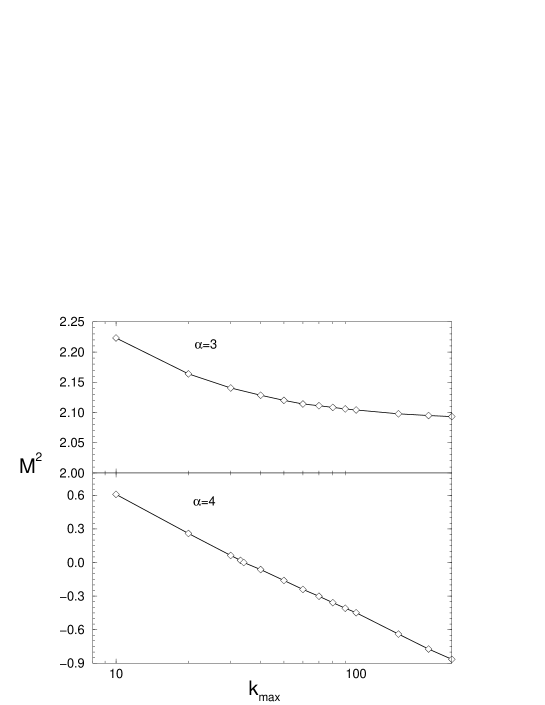
Figure 5: Cutoff dependence of the binding energy in the $J=0$ or $(1+,2-)$ state, in the one-channel problem ($f_{1}$), for two fixed values of the coupling constant below and above the critical value.

We have plotted in Figure 5 the mass square $M^{2}$ of the two fermion system as a function of the cutoff $k_{max}$ for two fixed values of the coupling constant below and above the critical value $\alpha_{c}=3.72$. In our calculations the cutoff appears directly as the maximum value $k_{max}$ up to which the integrals in (III) are performed. One can see two dramatically different behaviors depending on the value of the coupling constant $\alpha$. For $\alpha=3$, the result is convergent. On the contrary, for $\alpha=4$, i.e. $\alpha>\alpha_{c}$, the result is clearly divergent: $M^{2}$ decreases logarithmically as a function of $k_{max}$ and becomes even negative. This divergence is due only to the large $k$ behavior of $K_{11}$. Though the negative values of $M^{2}$ are physically meaningless, they are formally allowed by the equations (III) and (V). The first degree of $M$ does not enter neither in the equation nor in the kernel, and $M^{2}$ crosses zero without any singularity. The value of the critical $\alpha$ does not depend on the exchange mass $\mu$. For $\mu\ll m$, e.g. $\mu\approx 0.25$, its existence is not relevant in describing physical states since any solution with positive $M^{2}$, stable relative to cutoff, corresponds to $\alpha<\alpha_{c}$. For $\mu\sim m$ one can reach the critical $\alpha$ for positive, though small values of $M^{2}$.

Let us consider now the two-channel problem. The kernel dominating in asymptotics is $K_{22}$. In the case $J=0$ it is positive and corresponds to repulsion. Because of that, this kernel does not generate by itself any instability but cannot prevent from the collapse in the first channel (for enough large $\alpha$), since due to coupling between the two channels the singular potential in channel 1 ”pumps out” the wave function from channel 2. We would like to emphasize that the divergence in the $J=0$ case, when it happens, is not associated with the non decreasing behavior of the $K_{22}$ kernel but with the existence of a critical value of the coupling constant separating two dynamical regimes. This property is due only to the attraction and large $k$ behavior of $K_{11}$.

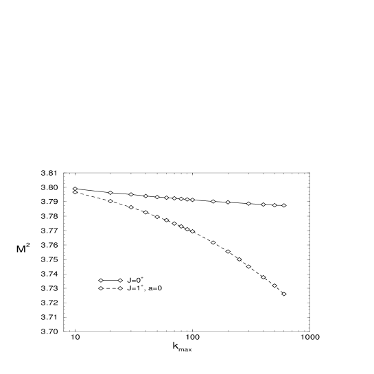
Figure 6: Cutoff dependence of $M^{2}$ for $J=0$ $(1+,2-)$ and $J=1,a=0$ $(1-,2+)$ states, in full (two-channel) problem, for $\alpha=1.184$.

In the coupled equations system (III) the situation with the cutoff dependence is thus the same as for one channel. In Figure 6 is displayed the variation of $M^{2}$ for $J=0$ – or $(1+,2-)$ and $J=1,a=0$ – or $(1-,2+)$ states as a function of the cutoff $k_{max}$. The value of the coupling constant is $\alpha=1.184$, the same that in Figure 2 of glazek1 , below the critical value. Our numerical results are in agreement with those presented in this figure for a cutoff $\Lambda\leq 100$, but our calculation at larger $k_{max}$ leads to different conclusion for the $J=0$ state. One remarks a qualitatively different behavior of the two states. In what concerns $J=0$, the numerical results become flatter when $k_{max}$ increases, with less than a 0.5% variation in $M^{2}$ when changing $k_{max}$ between $k_{max}$=10 and 300. The same kind of behavior is manifested when studying the cutoff dependence of the coupling constant for a fixed value of the binding energy. Figures 8 and 8 show the $\alpha(k_{max})$ variation for B=0.05 and B=0.5.

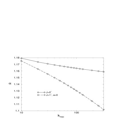
Figure 7: Cutoff dependence of the coupling constant, for $J=0$ and $J=1,a=0$ states, in full (two-channel) problem, for $B=0.05$.

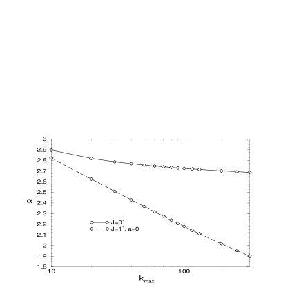
Figure 8: Cutoff dependence of the coupling constant, for $J=0$ and $J=1,a=0$ states, in full (two-channel) problem, for $B=0.5$.

The J=0 state is very well fitted by a law $\alpha(k_{max})=\alpha_{\infty}+{\alpha_{0}\over k_{max}^{\nu}}$ with parameters $\alpha_{\infty}=1.140$, $\alpha_{0}=0.0639$ and $\nu=0.210$ for B=0.05 and $\alpha_{\infty}=2.648$, $\alpha_{0}=0.809$ and $\nu=0.514$ for B=0.50. We thus conclude to the stability of the state with $J=0$, as expected from our analysis in section VI.

Figure 9: Asymptotic behavior of the J=0 wave function components $f_{i}$ for $B$=0.05, $\alpha$=1.096, $\mu$=0.25. The slope coefficient are $\beta_{1}=0.82$ and $\beta_{2}\approx 0$.

Figure 10: Asymptotic behavior of the J=0 wave function components $f_{i}$ for $B$=0.5, $\alpha$=2.48, $\mu$=0.25. The slope coefficient are $\beta_{1}=0.55$ and $\beta_{2}\approx 0$.

We have examined the asymptotic behavior of the wave function and found that it accurately follows the power law (80) with a coefficient $\beta(\alpha)$ given in Figure 4. For instance for a binding energy B=0.05 ($\alpha=1.096$) a direct measurement in the numerical solution plotted in Figure 10 gives $\beta=0.820\pm 0.002$ whereas the solution of equation (84) for the corresponding $\alpha$ gives $\beta=0.819$. The same kind of agreement was found for B=0.5 ($\alpha=2.480$): the asymptotic wave function – displayed in Figure 10 – gives $\beta=0.548\pm 0.002$ and equation (84) provides the value $\beta=0.547$. This agreement shows in particular that the critical value of the coupling constant is the same for the one- and the two-channel problem. The influence of the second channel seems to have no any effect in the asymptotic behavior of $f_{1}$. This channel behaves asymptotically as ${1/k^{2}}$ i.e. $\beta=0$ for any value of the binding energy, as indicated in sect. VI. One can see that the component $f_{2}$ changes the sign.

It is worth noticing that – at least in the framework of this model – one could measure the coupling constant from the asymptotic behavior of the bound state wave function. We would like to point out however that the extraction of coefficient $\beta$ is numerically delicate when solving the equation with finite values of the cutoff $k_{max}$. A way to overcome this difficulty consists in mapping the interval $k\in[0,\infty]$ into a compact interval. The mapping $k\rightarrow x={k\over k+m}$ was used.

Let us now consider the $J=1$ case. For $J=1,a=0$ or $(1-,2+)$ state, contrary to the $J=0$, the value of $M^{2}(k_{max})$ – displayed in Figure 6 – decreases faster than logarithmically and indicates a collapse. The asymptotics of the kernel $K^{(J=1)}_{22}$ is the same than $-K^{(J=0)}_{22}$, it is negative and corresponds to attraction. The integral (83) for the kernel $H(z,z^{\prime})$ with the function $A_{22}$ given by (78) diverges. Therefore it results in a collapse for any value of the coupling constant, as pointed out in glazek1 . The same result was found when solving the $J=0$ equations with the opposite sign of $K^{(J=0)}_{22}$. The case $J=1,a=1$ state requires a four channel calculations. The results displayed in Figure 11 show a logarithmic divergence.

Figure 11: Cutoff dependence of the coupling constant for $J=1,a=1$ state with $B=0.05$ until $k_{max}$=300. It shows a logarithmic divergence.

One can see from Figures 8 and 11 that the binding energies for the $J=1$ states with different values of projection $a$ are different but almost degenerate for a wide range of cutoff variation. For instance, with $k_{max}=10$ one has $\alpha_{a=0}$=1.17 $\alpha_{a=1}$=1.18 and with $k_{max}=90$, $\alpha_{a=0}$=1.14 $\alpha_{a=1}$=1.16. These differences are less than 1% for a system with not so small binding energies (B=0.05) and we expect them to be negligible for weakly bound systems like deuteron. This quasi-degeneracy is much smaller in comparison to the results previously found with the scalar particles heidelberg ; Taiwan ; Miller . In this latter case, a bound state with the same energy presents a splitting of $\approx 20\%$ in $\alpha$, what correspond to a energy difference $\Delta B\approx B$. It is worth noticing that even for the sizeable cutoff $k_{max}=90$, the value of the coupling constant is still $\approx$ 10% far from the converged one obtained by a mapping.

The 2+4 components of the $J=1^{+}$ state are displayed in Figures 13 and 13 as functions of the momentum $k$ .

Figure 12: Components $g_{1}$ and $g_{2}$ of the $J=1,a=0$ $(1-,2+)$ state, for $B=0.05$.

Figure 13: The four components $g_{i}$ of the $J=1,a=1$ $(1+,2-)$ state, for $B=0.05$.

Solutions $g_{1}$ and $g_{2}$ coming from the $a=0$ sector are comparable. They both depend on the angle $\theta$ between the direction of the light-front plane and the momentum $\vec{k}$: when $\vec{k}\perp\hat{n}$, the first component vanishes and the second one reaches its maximal value as a function of $\theta$: it dominates even over $g_{1}(k,\theta=0)$ and in the whole range of momentum. In the $J=1,a=0$ state, only one solution is sizeable and dominates the three others for all values of $\theta$. We would like to notice that the displayed components are related to the physical wave functions considered in ckj1 by some specific linear combinations ensuring the correct transformation properties of the wave function, as well as an easy link with the non relativistic solutions. The peculiarities of these functions and their relations will be discussed in a forthcoming paper fermions .

VIII Conclusion

The Light-Front solutions of the two fermion system interacting via a scalar exchange have been obtained. We have found that the $J=0$ – or $(1+,2-)$ – state is stable (i.e. convergent relative to the cutoff $k_{max}\to\infty$) for coupling constant below some critical value, in a way similar to what is known in non relativistic quantum mechanics for the $-\alpha^{\prime}/r^{2}$ potential. In this point, our conclusion differs from the one settled in glazek1 , where it was stated that the integrals in eqs. (V) diverge logarithmically with cutoff. Above the critical value the system collapses. This fact manifests as an unbounded value of $M^{2}$ when the cutoff tends to infinity.

We have shown analytically that the asymptotic behavior of the wave function has the form ${1\over k^{2+\beta}}$ and that the relation between coefficient $\beta$ and the coupling constant can be obtained as a solution of an eigenvalue equation suggested by smirnov . This relation provides in particular the critical value of the coupling constant, which corresponds to $\beta=0$. These results are in agreement with the numerical solutions of the LFD equations.

In the $J=1,a=0$ – or $(1-,2+)$ – state the system is found to be always unstable, as it was pointed out in glazek1 . The instability is related to the dominating $K_{22}$ kernel which is attractive. The origin of the collapse is thus different from $J=0$ state, for which the $K_{22}^{(J=0)}$ kernel is repulsive and the instability is due to the asymptotic behavior of attractive $K_{11}$ and depends on the value of $\alpha$ relative to $\alpha_{c}$.

The solutions for the four channel problem $J=1,a=1$ state have been obtained. They show also a logarithmic divergence of $M^{2}(k_{max})$ and are thus unstable without regularization.

These results should be taken into account when carrying out the renormalization procedure. The explicitly covariant version of Light-Front Dynamics (CLFD) seems very promising for handling this problem dugne , like it has proved to be fruitful in the Yukawa model.

Appendix A Explicit expressions for LFD kernels

The kernels are obtained through the traces (23). To calculate them, we express the scalar products between the different four-vectors in terms of variables $k,k^{\prime},\theta,\theta^{\prime},\varphi^{\prime}$. The following results are useful:

$$\omega^{2}=0$$

$$k_{1}^{2}=k_{2}^{2}=k^{\prime 2}_{1}=k^{\prime 2}_{2}=m^{2},$$

$$\omega\makebox[2.27626pt]{$\cdot$}k_{1}=x\;\omega\makebox[2.27626pt]{$\cdot$}p,$$

$$\omega\makebox[2.27626pt]{$\cdot$}k_{2}=(1-x)\omega\makebox[2.27626pt]{$\cdot$}p,$$

$$\omega\makebox[2.27626pt]{$\cdot$}k^{\prime}_{1}=x^{\prime}\omega\makebox[2.27626pt]{$\cdot$}p,$$

$$\omega\makebox[2.27626pt]{$\cdot$}k^{\prime}_{2}=(1-x^{\prime})\omega\makebox[2.27626pt]{$\cdot$}p,$$

$$k_{1}\makebox[2.27626pt]{$\cdot$}k_{2}=2\varepsilon_{k}^{2}-m^{2},$$

$$k^{\prime}_{1}\makebox[2.27626pt]{$\cdot$}k^{\prime}_{2}=2\varepsilon_{k^{\prime}}^{2}-m^{2},$$

$$k_{1}\makebox[2.27626pt]{$\cdot$}p=2\varepsilon_{k}^{2}(1-x)+M^{2}x/2,$$

$$k_{2}\makebox[2.27626pt]{$\cdot$}p=2\varepsilon_{k}^{2}x+M^{2}(1-x)/2$$

$$k^{\prime}_{1}\makebox[2.27626pt]{$\cdot$}p=2\varepsilon_{k^{\prime}}^{2}(1-x^{\prime})+M^{2}x^{\prime}/2,$$

$$k^{\prime}_{2}\makebox[2.27626pt]{$\cdot$}p=2\varepsilon_{k^{\prime}}^{2}x^{\prime}+M^{2}(1-x^{\prime})/2,$$

$$k_{1}\makebox[2.27626pt]{$\cdot$}k^{\prime}_{1}=-kk^{\prime}\sin\theta\sin\theta^{\prime}\cos\varphi^{\prime}+2\varepsilon_{k^{\prime}}^{2}x+2\varepsilon_{k}^{2}x^{\prime}-2\varepsilon_{k}^{2}xx^{\prime}-2\varepsilon_{k^{\prime}}^{2}xx^{\prime},$$

$$k_{2}\makebox[2.27626pt]{$\cdot$}k^{\prime}_{2}=-kk^{\prime}\sin\theta\sin\theta^{\prime}\cos\varphi^{\prime}+2\varepsilon_{k}^{2}x+2\varepsilon_{k^{\prime}}^{2}x^{\prime}-2\varepsilon_{k}^{2}xx^{\prime}-2\varepsilon_{k^{\prime}}^{2}xx^{\prime},$$

$$k_{1}\makebox[2.27626pt]{$\cdot$}k^{\prime}_{2}=kk^{\prime}\sin\theta\sin\theta^{\prime}\cos\varphi^{\prime}+2\varepsilon_{k}^{2}(1-x)(1-x^{\prime})+2\varepsilon_{k^{\prime}}^{2}xx^{\prime},$$

$$k_{2}\makebox[2.27626pt]{$\cdot$}k^{\prime}_{1}=kk^{\prime}\sin\theta\sin\theta^{\prime}\cos\varphi^{\prime}+2\varepsilon_{k^{\prime}}^{2}(1-x)(1-x^{\prime})+2\varepsilon_{k}^{2}xx^{\prime},$$

where $2x=\left(1-{k\cos\theta\over\varepsilon_{k}}\right)$ and similarly for $x^{\prime}$.

The analytical expressions for the $\kappa_{ij}$ kernels (23) in the $J=0$ case are:

$$\kappa_{11} = -\alpha\pi\left[2k^{2}k^{\prime 2}+3k^{2}m^{2}+3k^{\prime 2}m^{2}+4m^{4}-2kk^{\prime}\varepsilon_{k}\varepsilon_{k^{\prime}}\cos\theta\cos\theta^{\prime}-kk^{\prime}(\varepsilon_{k}^{2}+\varepsilon_{k^{\prime}}^{2})\sin\theta\sin\theta^{\prime}\cos\varphi^{\prime}\right]$$

$$\kappa_{12} = -\alpha\pi m(k^{2}-k^{\prime 2})\left(k^{\prime}\sin\theta^{\prime}+k\sin\theta\cos\varphi^{\prime}\right)$$

$$\kappa_{21} = -\alpha\pi m(k^{\prime 2}-k^{2})\left(k\sin\theta+k^{\prime}\sin\theta^{\prime}\cos\varphi^{\prime}\right)$$ (88)

$$\kappa_{22} = -\alpha\pi\left[\left(2k^{2}k^{\prime 2}+3k^{2}m^{2}+3k^{\prime 2}m^{2}+4m^{4}-2kk^{\prime}\varepsilon_{k}\varepsilon_{k^{\prime}}\cos\theta\cos\theta^{\prime}\right)\cos\varphi^{\prime}-kk^{\prime}(\varepsilon_{k}^{2}+\varepsilon_{k^{\prime}}^{2})\sin\theta\sin\theta^{\prime}\right]$$

where we have used $\alpha={g^{2}\over 4\pi}$.

The analytical expressions for the $\kappa_{ij}$ kernels (33) in the $J=1^{+},a=0$ case are:

$$\kappa_{11} = -\alpha\pi\left\{\left[-2kk^{\prime}\varepsilon_{k}\varepsilon_{k^{\prime}}+(2k^{2}k^{\prime 2}+3m^{2}k^{2}+3m^{2}k^{\prime 2}+4m^{4})\cos\theta\cos\theta^{\prime}\right]+\varepsilon_{k}\varepsilon_{k^{\prime}}(k^{2}+k^{\prime 2}+4m^{2})\sin\theta\sin\theta^{\prime}\cos\varphi^{\prime}\right\}$$

$$\kappa_{12} = -\alpha\pi m\left[-\varepsilon_{k^{\prime}}(3k^{2}+k^{\prime 2}+4m^{2})\cos\theta\sin\theta^{\prime}+\varepsilon_{k}(k^{2}+3k^{\prime 2}+4m^{2})\sin\theta\cos\theta^{\prime}\cos\varphi^{\prime}\right]$$

$$\kappa_{21} = -\alpha\pi m\left[-\varepsilon_{k}(k^{2}+3k^{\prime 2}+4m^{2})\sin\theta\cos\theta^{\prime}+\varepsilon_{k^{\prime}}(3k^{2}+k^{\prime 2}+4m^{2})\cos\theta\sin\theta^{\prime}\cos\varphi^{\prime}\right]$$ (89)

$$\kappa_{22} = -\alpha\pi\left\{\varepsilon_{k}\varepsilon_{k^{\prime}}(k^{2}+k^{\prime 2}+4m^{2})\sin\theta\sin\theta^{\prime}+\left[-2kk^{\prime}\varepsilon_{k}\varepsilon_{k^{\prime}}+(2k^{2}k^{\prime 2}+3m^{2}k^{2}+3m^{2}k^{\prime 2}+4m^{4})\cos\theta\cos\theta^{\prime}\right]\cos\varphi^{\prime}\right\}$$

The analytical expressions for the $\kappa_{ij}$, determining by eq. (22) the kernels $K_{ij}$ in the $J=1^{+},a=1$ case are:

$${2\kappa_{11}\over\alpha\pi} = -m[\varepsilon_{k}\sin^{2}\theta(\varepsilon_{k}^{2}+3\varepsilon_{k^{\prime}}^{2})+\varepsilon_{k^{\prime}}\sin^{2}\theta^{\prime}(3\varepsilon_{k}^{2}+\varepsilon_{k^{\prime}}^{2})]-(\cos^{2}\theta+\cos^{2}\theta^{\prime})[m^{2}(\varepsilon_{k}^{2}+\varepsilon_{k^{\prime}}^{2})+2\varepsilon_{k}^{2}\varepsilon_{k^{\prime}}^{2}]+4\varepsilon_{k}\varepsilon_{k^{\prime}}kk^{\prime}\cos\theta\cos\theta^{\prime}$$

$$- (\varepsilon_{k}+\varepsilon_{k^{\prime}})^{2}\sin\theta\sin\theta^{\prime}\cos\varphi^{\prime}\left\{(\varepsilon_{k}-m)(\varepsilon_{k^{\prime}}-m)[\cos\theta\cos\theta^{\prime}+\sin\theta\sin\theta^{\prime}\cos\varphi^{\prime}]-kk^{\prime}\right\}$$

$${2\kappa_{12}\over\alpha\pi} = m\varepsilon_{k}(\varepsilon_{k}^{2}+3\varepsilon_{k^{\prime}}^{2})\sin^{2}\theta-m\varepsilon_{k^{\prime}}(3\varepsilon_{k}^{2}+\varepsilon_{k^{\prime}}^{2})\sin^{2}\theta^{\prime}+(\cos^{2}\theta-\cos^{2}\theta^{\prime})[m^{2}\varepsilon_{k}^{2}+m^{2}\varepsilon_{k^{\prime}}^{2}+2\varepsilon_{k}^{2}\varepsilon_{k^{\prime}}^{2}]$$

$$- \sin\theta\sin\theta^{\prime}\left\{kk^{\prime}(\varepsilon_{k}-\varepsilon_{k^{\prime}})^{2}+(\varepsilon_{k}+\varepsilon_{k^{\prime}})^{2}(\varepsilon_{k^{\prime}}-m)(\varepsilon_{k^{\prime}}-m)\cos\theta\cos\theta\right\}\cos\varphi^{\prime}$$

$$+ \sin^{2}\theta(\varepsilon_{k}-m)\left\{-(\varepsilon_{k^{\prime}}+m)(\varepsilon_{k}-\varepsilon_{k^{\prime}})^{2}+(\varepsilon_{k^{\prime}}-m)(\varepsilon_{k}+\varepsilon_{k^{\prime}})^{2}\cos^{2}\theta^{\prime}\right\}\cos^{2}\varphi^{\prime}$$

$${2\kappa_{13}\over\sqrt{2}\alpha\pi} = -\sin\theta^{\prime}\left[2\varepsilon_{k}\varepsilon_{k^{\prime}}kk^{\prime}\cos\theta+(\varepsilon_{k^{\prime}}-m)[m(\varepsilon_{k^{\prime}}^{2}+\varepsilon_{k}^{2})-2\varepsilon_{k}^{2}\varepsilon_{k^{\prime}}]\cos\theta^{\prime}\right]$$

$$+ \sin\theta\left\{2\varepsilon_{k}\varepsilon_{k^{\prime}}kk^{\prime}\cos\theta^{\prime}+(\varepsilon_{k}-m)\cos\theta\left[\varepsilon_{k^{\prime}}(\varepsilon_{k}^{2}+\varepsilon_{k^{\prime}}^{2}-2m\varepsilon_{k})-(\varepsilon_{k^{\prime}}-m)(\varepsilon_{k}+\varepsilon_{k^{\prime}})^{2}\cos^{2}\theta^{\prime}\right]\right\}\cos\varphi^{\prime}$$

$$- (\varepsilon_{k}+\varepsilon_{k^{\prime}})^{2}(\varepsilon_{k}-m)(\varepsilon_{k^{\prime}}-m)\sin^{2}\theta\sin\theta^{\prime}\cos\theta^{\prime}\cos^{2}\varphi^{\prime}$$

$${2\kappa_{14}\over\alpha\pi} = \sqrt{2}(k^{2}-k^{\prime 2})\left\{(\varepsilon_{k}\sin^{2}\theta+m\cos^{2}\theta)k^{\prime}\sin\theta^{\prime}+mk\sin\theta\cos\varphi^{\prime}-k^{\prime}(\varepsilon_{k}-m)\sin^{2}\theta\sin\theta^{\prime}\cos^{2}\varphi^{\prime}\right\}$$

$${2\kappa_{21}\over\alpha\pi} = -m\varepsilon_{k}\sin^{2}\theta(3\varepsilon^{2}_{k^{\prime}}+\varepsilon^{2}_{k})+m\varepsilon_{k^{\prime}}\sin^{2}\theta^{\prime}(\varepsilon^{2}_{k^{\prime}}+3\varepsilon^{2}_{k})-(\cos^{2}\theta-\cos^{2}\theta^{\prime})\left(m^{2}(\varepsilon^{2}_{k^{\prime}}+\varepsilon^{2}_{k})+2\varepsilon^{2}_{k^{\prime}}\varepsilon^{2}_{k}\right)$$

$$- \sin\theta\sin\theta^{\prime}\left\{kk^{\prime}(\varepsilon_{k}-\varepsilon_{k^{\prime}})^{2}+(\varepsilon_{k}+\varepsilon_{k^{\prime}})^{2}(\varepsilon_{k^{\prime}}-m)(\varepsilon_{k}-m)\cos\theta\cos\theta^{\prime}\right\}\cos\varphi^{\prime}$$

$$+ \sin^{2}\theta^{\prime}(\varepsilon_{k^{\prime}}-m)\left\{-(\varepsilon_{k^{\prime}}-\varepsilon_{k})^{2}(\varepsilon_{k}+m)+\cos^{2}\theta(\varepsilon_{k^{\prime}}+\varepsilon_{k})^{2}(\varepsilon_{k}-m)\right\}\cos^{2}\varphi^{\prime}$$

$${2\kappa_{22}\over\alpha\pi} = m(\varepsilon_{k}+\varepsilon_{k^{\prime}})^{3}-(\varepsilon_{k}-m)(m(\varepsilon^{2}_{k}+\varepsilon^{2}_{k^{\prime}})-2\varepsilon_{k}\varepsilon^{2}_{k^{\prime}})\cos^{2}\theta-(\varepsilon_{k^{\prime}}-m)(m(\varepsilon^{2}_{k}+\varepsilon^{2}_{k^{\prime}})-2\varepsilon^{2}_{k}\varepsilon_{k^{\prime}})\cos^{2}\theta^{\prime}$$

$$- 4kk^{\prime}\varepsilon_{k}\varepsilon_{k^{\prime}}\cos\theta\cos\theta^{\prime}-(\varepsilon_{k}+\varepsilon_{k^{\prime}})^{2}\left\{(\varepsilon_{k}-m)(\varepsilon_{k^{\prime}}-m)-kk^{\prime}\cos\theta\cos\theta^{\prime}\right\}\sin\theta\sin\theta^{\prime}\cos\varphi^{\prime}$$

$$- \left\{\sin^{2}\theta^{\prime}\left(\sin^{2}\theta\varepsilon_{k}\varepsilon_{k^{\prime}}(\varepsilon^{2}_{k}+\varepsilon^{2}_{k^{\prime}}+2m^{2})+m\varepsilon_{k^{\prime}}(\cos^{2}\theta+1)(3\varepsilon^{2}_{k}+\varepsilon^{2}_{k^{\prime}})\right)+(\cos^{2}\theta^{\prime}+1)\right.$$

$$\times \left.\left(m\varepsilon_{k}\sin^{2}\theta(\varepsilon^{2}_{k}+3\varepsilon^{2}_{k^{\prime}})+(\cos^{2}\theta+1)(m^{2}(\varepsilon^{2}_{k}+\varepsilon^{2}_{k^{\prime}})+2\varepsilon^{2}_{k}\varepsilon^{2}_{k^{\prime}})\right)-8kk^{\prime}\varepsilon_{k}\varepsilon_{k^{\prime}}\cos\theta\cos\theta^{\prime}\right\}\cos^{2}\varphi^{\prime}$$

$${2\kappa_{23}\over\sqrt{2}\alpha\pi} = \left\{2\varepsilon_{k}\varepsilon_{k^{\prime}}k^{\prime}k\cos\theta+(\varepsilon_{k^{\prime}}-m)\cos\theta^{\prime}(\varepsilon^{2}_{k^{\prime}}m+\varepsilon^{2}_{k}(m-2\varepsilon_{k^{\prime}}))\right\}\sin\theta^{\prime}-\sin\theta$$

$$\times \left\{(\varepsilon_{k}-m)\cos\theta\left((\varepsilon_{k}+\varepsilon_{k^{\prime}})^{2}(\varepsilon_{k^{\prime}}-m)\cos^{2}\theta^{\prime}-\varepsilon_{k^{\prime}}(\varepsilon^{2}_{k}+\varepsilon^{2}_{k^{\prime}}-2m\varepsilon_{k})\right)-2kk^{\prime}\varepsilon_{k}\varepsilon_{k^{\prime}}\cos\theta^{\prime}\right\}\cos\varphi^{\prime}$$

$$- \sin\theta^{\prime}\left\{(\varepsilon_{k^{\prime}}-m)\cos\theta^{\prime}\left((\varepsilon_{k}-\varepsilon_{k^{\prime}})^{2}(\varepsilon_{k}+m)-(\varepsilon_{k}+\varepsilon_{k^{\prime}})^{2}(\varepsilon_{k}-m)\cos^{2}\theta\right)+4kk^{\prime}\varepsilon_{k}\varepsilon_{k^{\prime}}\cos\theta\right\}\cos^{2}\varphi^{\prime}$$

$${2\kappa_{24}\over\alpha\pi} = \sqrt{2}(\varepsilon_{k^{\prime}}^{2}-\varepsilon_{k}^{2})\left\{mk\sin\theta\cos\varphi^{\prime}-k^{\prime}\sin\theta^{\prime}\left[(\varepsilon_{k}\sin^{2}\theta+m\cos^{2}\theta)-[(\varepsilon_{k}+m)-(\varepsilon_{k}-m)\cos^{2}\theta]\cos^{2}\varphi^{\prime}\right]\right\}$$

$${2\kappa_{31}\over\sqrt{2}\alpha\pi} = -\sin\theta\left[(\varepsilon_{k}-m)(m\varepsilon_{k}^{2}+m\varepsilon_{k^{\prime}}^{2}-2\varepsilon_{k}\varepsilon_{k^{\prime}}^{2})+2\varepsilon_{k}\varepsilon_{k^{\prime}}kk^{\prime}\cos\theta^{\prime}\right]$$

$$+ \sin\theta^{\prime}\left\{(\varepsilon_{k}-m)\cos\theta^{\prime}\left[(m\varepsilon_{k}^{2}+m\varepsilon_{k^{\prime}}^{2}-2\varepsilon_{k}^{2}\varepsilon_{k^{\prime}})\cos^{2}\theta+\varepsilon_{k}(\varepsilon_{k}^{2}+\varepsilon_{k^{\prime}}^{2}-2m\varepsilon_{k^{\prime}})\sin^{2}\theta\right]+2\varepsilon_{k}\varepsilon_{k^{\prime}}kk^{\prime}\cos\theta^{\prime}\right\}\cos\varphi^{\prime}$$

$$- (\varepsilon_{k}+\varepsilon_{k^{\prime}})^{2}(\varepsilon_{k}-m)(\varepsilon_{k^{\prime}}-m)\sin\theta\cos\theta\sin^{2}\theta^{\prime}\cos^{2}\varphi^{\prime}$$

$${2\kappa_{32}\over\sqrt{2}\alpha\pi} = \sin\theta\left[2\varepsilon_{k}\varepsilon_{k^{\prime}}kk^{\prime}\cos\theta^{\prime}+(e-m)[m(\varepsilon_{k}^{2}+\varepsilon_{k^{\prime}}^{2})-2\varepsilon_{k}\varepsilon_{k^{\prime}}^{2}]\cos\theta\right]$$

$$+ \sin\theta^{\prime}\cos\varphi^{\prime}\left\{(\varepsilon_{k^{\prime}}-m)\cos\theta^{\prime}\left[\cos^{2}\theta(m\varepsilon_{k}^{2}+m\varepsilon_{k^{\prime}}^{2}-2\varepsilon_{k}^{2}\varepsilon_{k^{\prime}}^{2})+\varepsilon_{k}\sin^{2}\theta[\varepsilon_{k}^{2}+\varepsilon_{k^{\prime}}^{2}-2m\varepsilon_{k^{\prime}}\right]+2\varepsilon_{k}\varepsilon_{k^{\prime}}kk^{\prime}\cos\theta\right\}$$

$$+ \sin\theta\cos^{2}\varphi^{\prime}\left\{(\varepsilon_{k}-m)\cos\theta\left[\varepsilon_{k^{\prime}}(2\varepsilon_{k}m-\varepsilon_{k}^{2}-\varepsilon_{k^{\prime}}^{2})\sin^{2}\theta^{\prime}+(2\varepsilon_{k}\varepsilon_{k^{\prime}}^{2}-m\varepsilon_{k}^{2}-m\varepsilon_{k^{\prime}}^{2})(1+\cos^{2}\theta^{\prime})\right]-4\varepsilon_{k}\varepsilon_{k^{\prime}}kk^{\prime}\cos\theta^{\prime}\right\}$$

$${\kappa_{33}\over\alpha\pi} = \left\{\varepsilon_{k}(\varepsilon_{k^{\prime}}-m)\left(\varepsilon^{2}_{k}+\varepsilon_{k^{\prime}}(\varepsilon_{k^{\prime}}-2m)\right)\cos^{2}\theta^{\prime}-\varepsilon_{k^{\prime}}m(3\varepsilon^{2}_{k}+\varepsilon^{2}_{k^{\prime}})\cos^{2}\theta-\varepsilon_{k}\varepsilon_{k^{\prime}}(\varepsilon^{2}_{k}+\varepsilon^{2}_{k^{\prime}}+2m^{2})\sin^{2}\theta\right.$$

$$- \left.\left((\varepsilon_{k}+\varepsilon_{k^{\prime}})^{2}(\varepsilon_{k}-m)(\varepsilon_{k^{\prime}}-m)\cos\theta\cos\theta^{\prime}-2kk^{\prime}\varepsilon_{k}\varepsilon_{k^{\prime}}\right)(\cos\theta\cos\theta^{\prime}+\sin\theta\sin\theta^{\prime}\cos\varphi^{\prime})\right\}\cos\varphi^{\prime}$$

$${\kappa_{34}\over\alpha\pi} = (\varepsilon_{k}^{2}-\varepsilon_{k^{\prime}}^{2})(\varepsilon_{k}-m)\cos\theta\sin\theta k^{\prime}\sin\theta^{\prime}\sin^{2}\varphi^{\prime}$$

$${2\kappa_{41}\over\alpha\pi} = \sqrt{2}(\varepsilon_{k^{\prime}}^{2}-\varepsilon_{k}^{2})\left\{mk^{\prime}\sin\theta^{\prime}\cos\varphi^{\prime}+k\sin\theta\left[(\varepsilon_{k^{\prime}}\sin^{2}\theta^{\prime}+m\cos^{2}\theta^{\prime})-(\varepsilon_{k^{\prime}}-m)\sin^{2}\theta^{\prime}\sin^{2}\varphi^{\prime}\right]\right\}$$

$${2\kappa_{42}\over\alpha\pi} = \sqrt{2}(\varepsilon_{k}^{2}-\varepsilon_{k^{\prime}}^{2})\left\{mk^{\prime}\sin\theta^{\prime}\cos\varphi^{\prime}+k\sin\theta\left[[(m+\varepsilon_{k^{\prime}})+(m-\varepsilon_{k^{\prime}})\cos^{2}\theta^{\prime}]\cos^{2}\varphi^{\prime}-(\varepsilon_{k^{\prime}}\sin^{2}\theta^{\prime}+m\cos^{2}\theta^{\prime})\right]\right\}$$

$${\kappa_{43}\over\alpha\pi} = -k(\varepsilon_{k}^{2}-\varepsilon_{k^{\prime}}^{2})(\varepsilon_{k^{\prime}}-m)\cos\theta^{\prime}\sin\theta\sin\theta^{\prime}\sin^{2}\varphi^{\prime}$$

$${\kappa_{44}\over\alpha\pi} = \left\{(\varepsilon_{k}^{2}+\varepsilon_{k^{\prime}}^{2})(kk^{\prime}\sin\theta\sin\theta^{\prime}\cos\varphi^{\prime}-m^{2})+2\varepsilon_{k}\varepsilon_{k^{\prime}}(kk^{\prime}\cos\theta\cos\theta^{\prime}-\varepsilon_{k}\varepsilon_{k^{\prime}})\right\}\cos\varphi^{\prime}$$

Appendix B Coefficients $\eta_{ij}$ determining the orthonormalized spin structures

The construction method of the four orthonormalized spin structures $S^{(1)}_{i\mu}$ (36) determining the wave function $\phi^{(1)}_{\mu}$ (35), is explained in These_MMB . These structures are expressed in terms of six structures $S_{j\mu}$, in the form (36). The non zero coefficients $\eta_{ij}$ ($i=1,\ldots,4;\;j=1,\ldots,6$) are given below ($z=\cos\theta$):

$$\eta_{11}=\frac{\sqrt{3}m^{2}}{4\varepsilon_{k}(\varepsilon_{k}+m)},\quad\eta_{12}=\frac{\sqrt{3}m}{4\varepsilon_{k}},\quad\eta_{13}=-\frac{\sqrt{3}(\varepsilon_{k}-m)(4\varepsilon_{k}^{2}+M^{2})z}{16\varepsilon_{k}^{2}k},$$

$$\eta_{16}=\frac{\sqrt{3}(4\varepsilon_{k}^{2}+M^{2})}{8\varepsilon_{k}m},$$

$$\eta_{21}=\frac{\sqrt{3}m^{2}[\varepsilon_{k}(1-z^{2})+m(1+z^{2})]}{4\varepsilon_{k}k^{2}(1-z^{2})},\quad\eta_{22}=-\frac{\sqrt{3}m}{4\varepsilon_{k}},$$

$$\eta_{23}=-\frac{\sqrt{3}(4\varepsilon_{k}^{2}+M^{2})[\varepsilon_{k}(1-z^{2})+m(1+z^{2})]z}{16\varepsilon_{k}^{2}k(1-z^{2})},\quad\eta_{24}=\frac{\sqrt{3}mz}{k(1-z^{2})},$$

$$\eta_{26}=-\frac{\sqrt{3}(4\varepsilon_{k}^{2}+M^{2})(1+z^{2})}{8\varepsilon_{k}m(1-z^{2})}$$

$$\eta_{31}=\frac{\sqrt{3}m^{2}z}{2\varepsilon_{k}(\varepsilon_{k}+m)\sqrt{2(1-z^{2})}},\quad\eta_{33}=-\frac{\sqrt{3}(\varepsilon_{k}-m)(4\varepsilon_{k}^{2}+M^{2})z^{2}}{8\varepsilon_{k}^{2}k\sqrt{2(1-z^{2})}},$$

$$\eta_{34}=-\frac{\sqrt{3}m}{k\sqrt{2(1-z^{2})}},\quad\eta_{36}=\frac{\sqrt{3}(4\varepsilon_{k}^{2}+M^{2})z}{4\varepsilon_{k}m\sqrt{2(1-z^{2})}}$$

$$\eta_{45}=\frac{\sqrt{3}m^{2}}{2\varepsilon_{k}k\sqrt{2(1-z^{2})}}$$ (90)

References

(1) S.J. Brodsky, H.-C. Pauli and S.S. Pinsky, Phys. Rep., 301 (1998) 299.
(2) St. Glazek, A. Harindranath, S. Pinsky, J. Shigemutsu and
K. Wilson, Phys. Rev. D47 (1993) 1599.
(3) St. Glazek and K.G. Wilson,
Phys. Rev. D47 (1993) 4657.
(4) R.J. Perry, A. Harindranath and K.G. Wilson, Phys. Rev. Lett., 65 (1990) 2959.