Abelian Higgs Hair for AdS-Schwarzschild Black Hole

M.H. Dehghani, A.M. Ghezelbash and R. B. Mann

Department of Physics, University of Waterloo,

Waterloo, Ontario N2L 3G1, CANADA

We show that the Abelian Higgs field equations in the background of the four dimensional AdS-Schwarzschild black hole have a vortex line solution. This solution, which has axial symmetry, is a generalization of the AdS spacetime Nielsen-Olesen string. By a numerical study of the field equations, we show that black hole could support the Abelian Higgs field as its Abelian hair. Also, we conside the self gravity of the Abelian Higgs field both in the pure AdS spacetime and AdS-Schwarzschild black hole background and show that the effect of string as a black hole hair is to induce a deficit angle in the AdS-Schwarzschild black hole.

1 Introduction

The classical no-hair conjecture first proposed by Ruffini and Wheeler [1] states that after a given distribution of matter collapses to form a black hole, the only long range information of a black hole is its electromagnetic charge, mass and angular momentum. In certain special cases the conjecture has been verified. For example a scalar field minimally coupled to gravity in asymptotically flat or de Sitter spacetimes cannot provide hair for the black hole [2],[3].

While it is tempting to extend the no-hair theorem claim to all forms of matter, it is known that some long range Yang-Mills and/or quantum hair could be painted on the black holes [4]. Explicit calculations have been carried out which verify the existence of a long range Nielsen-Olesen vortex solution as a stable hair for a Schwarzchild black hole in four dimensions [5], although it might be argued that this situation falls outside the scope of the classical no-hair theorem due to the non trivial topology of the string configuration. More recently it has been shown that an asymptotically flat black hole could be pierced by several infinitely thin cosmic strings in a polyhedral configuration [6]. These is much current interest in extending these considerations to anti de Sitter spacetime, mainly due to the efforts of  Maldacena [7] and Witten [8] concerning the relation of the some large ${\cal N}$ gauge theories in AdS spacetime and conformal field theories.

Insofar as the no-hair theorem is concerned it has been shown that there exists a solution to the $SU(2)$ Einstein-Yang-Mills equations which describes a stable Yang-Mills hairy black hole that is asymptotically AdS [4]. More recently we have shown that the $U(1)$ Higgs field equations have a vortex solution in four dimensional AdS spacetime [9].  More recently it has been shown that in asymptotically AdS spacetime, that a black hole can have scalar hair [10].

Motivated by these considerations, in this article we investigate possible solutions of the Abelian-Higgs field equations in a four dimensional AdS-Schwarzschild black hole background. While an analytical solution to these equations appears to be intractable, we confirm but by numerical calculation that AdS-Schwarzscild black hole could support a long range cosmic string as its stable hair. The generalization to the multi-string configurations as a black hole hairs also could be done.

In section two, we solve the first-order Einstein equations in the pure AdS₄ spacetime in the presence of a vortex solution. In section three, we solve numerically the Abelian-Higgs equations in the Ads-Schwarzschild background for different values of the cosmological constant and string winding numbers. In section four, by studying the behaviour of the string energy-momentum tensor, we find the effect of the vortex self gravity on the AdS-Schwarzschild background metric. We argue in section five, that AdS-Schwarzschild black hole could support a multi-string configuration. We give some closing remarks in the final section.

2 Vortex Self Gravity on AdS₄

We consider first the effect of  the vortex on the AdS₄ spacetime. This entails finding the solutions of the coupled Einstein-Abelian Higgs differential equations in AdS₄. This is a formidable problem even for flat spacetime, and no exact solutions have been found  for the flat spacetime yet.

However  some physical results can be obtained by making some approximations. First, we assume that the thickness of the vortex is much smaller that all the other relevant length scales. Second, we assume that the gravitational effects of the string are weak enough so that the linearized Einstein-Abelian Higgs differential equations are applicable.

For convenience, in this section we use the following form of the metric of AdS${}_{4}.$

$$ds^{2}=-\widetilde{A}(r,\theta)^{2}dt^{2}+\widetilde{B}(r,\theta)^{2}d\phi^{2}+\widetilde{C}(r,\theta)(\frac{dr^{2}}{1+\frac{r^{2}}{l^{2}}}+r^{2}d\theta^{2})$$ (1)

This metric in spherical coordinates is suitable for generalizing the vortex self gravity in the presence of the AdS-Schwarzschild black hole. In the absence of the vortex, we must have $A_{0}(r,\theta)=\sqrt{1+\frac{r^{2}}{l^{2}}},B_{0}(r,\theta)=r\sin\theta,C_{0}(r,\theta)=1$ , yielding the well known metric of pure AdS₄.

Employing the two assumptions concerning the thickness of the vortex core and its weak gravitational field, we solve numerically the Einstein field equations,

$$G_{\mu\nu}-\frac{3}{l^{2}}g_{\mu\nu}=-8\pi G{\cal T}_{\mu\nu}$$ (2)

to the first order in $\varepsilon=8\pi G,$ where ${\cal T}_{\mu\nu}$ is the energy-momentum tensor of the Abelian Higgs field in the AdS background. To first order of approximation by taking $g_{\mu\nu}\simeq g_{\mu\nu}^{(0)}+g_{\mu\nu}^{(1)}$ , where $g_{\mu\nu}^{(0)}$ is the usual AdS${}_{4\text{ }}$ metric, $\ g_{\mu\nu}^{(1)}$ is the first order correction to the metric and writing

$$\widetilde{A}(r,\theta)=A_{0}(r,\theta)(1+\varepsilon A(r,\theta))$$

(3)

we obtain corrections to the three functions $A_{0}(r,\theta),B_{0}(r,\theta)$ and $C_{0}(r,\theta)$ in (3). Hence in the first approximation the equations (2) become

$$G_{\mu\nu}^{(1)}-\frac{3}{l^{2}}g_{\mu\nu}^{(1)}=-{\cal T}_{\mu\nu}^{(0)}$$ (4)

where ${\cal T}_{\mu\nu}^{(0)}$ is the energy momentum tensor of string field in AdS${}_{4\text{ }}$background metric, and $G_{\mu\nu}^{(1)}$ is the correction to the Einstein tensor due to $g_{\mu\nu}^{(1)}$.

The rescaled components of the energy momentum tensor of string in the background of AdS${}_{4},$ are given by,

$$T_{t}^{t(0)}(\rho)=-\frac{1}{2}(\frac{dX}{d\rho})^{2}(1+\frac{\rho^{2}}{l^{2}})-\frac{1}{2}\frac{1}{\rho^{2}}(\frac{dP}{d\rho})^{2}(1+\frac{\rho^{2}}{l^{2}})-\frac{1}{2}\frac{P^{2}X^{2}}{\rho^{2}}-(X^{2}-1)^{2}$$

(5)

where $X$ and $P$ are the solutions of  the string fields [9] and $\rho=r\sin\theta$.

The Einstein equations (4) are

$$(1+\frac{\rho^{2}}{l^{2}})\frac{d^{2}B}{d\rho^{2}}+2\frac{dB}{d\rho}(\frac{1}{\rho}+\frac{2\rho}{l^{2}})+\frac{1}{2}(1+\frac{\rho^{2}}{l^{2}})\frac{d^{2}C}{d\rho^{2}}+\frac{\rho}{l^{2}}\frac{dC}{d\rho}-\frac{3C}{l^{2}}=T_{t}^{t(0)}$$

(6)

Solving equations of motions of the Abelian Higgs fields [9] numerically gives the following graphs for $X$ and $P$ fields (1)

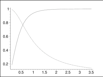
Figure 1: $X(\rho)$ (solid) and $P(\rho)$ (dotted) for $l=1$

By using the equations (5), one could obtain the diagram (2) showing the behaviour of stress tensor components.

Figure 2: $T_{t}^{t(0)}$(solid),$T_{\varphi}^{\varphi(0)}$(dashed)$,T_{r}^{r(0)}+T_{\theta}^{\theta(0)}$ (dash-dotted) curves for $l=1$

Then solving the coupled differential equations (6) gives the behaviour of functions $A(\rho),B(\rho)$ and $C(\rho)$ versus $\rho.$ (3)

Figure 3: $A$(solid),$B$(dotted)$,C$ touches the horizontal axis

Hence by a redefinition of time coordinate in (1) the metric can be rewritten as

$$ds^{2}=-(1+\frac{r^{2}}{l^{2}})dt^{2}+\frac{dr^{2}}{1+\frac{r^{2}}{l^{2}}}+r^{2}(d\theta^{2}+\alpha^{2}\sin^{2}\theta d\phi^{2})$$ (7)

which is the metric of AdS space with deficit angle.

3 Abelian Higgs Vortex in AdS$-$Schwarzschild Black Hole

We take the Abelian Higgs Lagrangian in AdS-Schwarzschild as follows,

$${\cal L}(\Phi,A_{\mu})=-\frac{1}{2}({\cal D}_{\mu}\Phi)^{\dagger}{\cal D}^{\mu}\Phi-\frac{1}{16\pi}{\cal F}_{\mu\nu}{\cal F}^{\mu\nu}-\xi(\Phi^{\dagger}\Phi-\eta^{2})^{2}$$ (8)

where $\Phi$ is a complex  scalar Klein-Gordon field, ${\cal F}_{\mu\nu}$ is the field strength of  the electromagnetic field $A_{\mu}$ and ${\cal D}_{\mu}=\nabla_{\mu}+ieA_{\mu}$ in which $\nabla_{\mu}$ is the covariant derivative. We employ Planck units $G=\hbar=c=1$ which implies that the Planck mass is equal to unity, and write the AdS-Schwarzschild black hole metric in the form

$$ds^{2}=-(1-\frac{2m}{r}+\frac{r^{2}}{l^{2}})dt^{2}+\frac{1}{(1-\frac{2m}{r}+\frac{r^{2}}{l^{2}})}dr^{2}+r^{2}(d\theta^{2}+\sin^{2}\theta\,d\varphi^{2})$$ (9)

where $\ m$ is the black hole mass and the cosmological constant $\Lambda$ is equal to $\frac{-3}{l^{2}}.$ Defining the real fields $X(x^{\mu}),\omega(x^{\mu}),P_{\mu}(x^{\nu})$ by the following equations

$$\Phi(x^{\mu})=\eta X(x^{\mu})e^{i\omega(x^{\mu})}$$

(10)

and employing a suitable choice of gauge, one could rewrite the Lagrangian ( 8) and the equations of motion in terms of these fields as:

$${\cal L(}X,P_{\mu})=-\frac{\eta^{2}}{2}(\nabla_{\mu}X\,\nabla^{\mu}X+X^{2}P_{\mu}P^{\mu})-\frac{1}{16\pi e^{2}}F_{\mu\nu}F^{\mu\nu}-\xi\eta^{4}(X^{2}-1)^{2}$$ (11)

$$\nabla_{\mu}\nabla^{\mu}X-XP_{\mu}P^{\mu}-4\xi\eta^{2}X(X^{2}-1)=0$$

(12)

where $F^{\mu\nu}=\nabla^{\mu}P^{\nu}-\nabla^{\nu}P^{\mu}$ is the field strength of the corresponding gauge field $P^{\mu}$. Note that the real field $\omega$ is not itself a physical quantity. Superficially it appears not to contain any physical information. However if $\omega$ is not single valued this is no longer the case, and the resultant solutions are referred to as vortex solutions [14].  In this case the requirement that $\Phi$ field be single-valued implies that the line integral of $\omega$ over any closed loop is $\pm 2\pi n$ where $n$ is an integer. In this case the flux of electromagnetic field $\Phi_{H\text{ \ }}$passing through such a closed loop is quantized with quanta $2\pi/e.$

We seek a vortex solution for the Abelian Higgs Lagrangian (11) in the background of AdS-Schwarzschild black hole.This solution can be interpreted as a string piercing to the black hole (9). Considering the static case of winding number $N$ with the gauge choice,

$$P_{\mu}(r,\theta)=(0;0,0,NP(r,\theta))$$ (13)

and rescaling

$$\varkappa\rightarrow\frac{\varkappa}{\sqrt{\xi}\eta}$$ (14)

where $\varkappa=r,l,m,$ the equations of motion (12) are

$$(1-\frac{2m}{r}+\frac{r^{2}}{l^{2}})\frac{\partial^{2}X(r,\theta)}{\partial r^{2}}+\frac{2}{r}(1-\frac{m}{r}+\frac{2r^{2}}{l^{2}})\frac{\partial X(r,\theta)}{\partial r}+\frac{1}{r^{2}}\frac{\partial^{2}X(r,\theta)}{\partial\theta^{2}}+\frac{1}{r^{2}}\frac{\partial X(r,\theta)}{\partial\theta}\cot\theta-\frac{1}{2}(X^{3}(r,\theta)$$

(15)

$$(1-\frac{2m}{r}+\frac{r^{2}}{l^{2}})\frac{\partial^{2}P(r,\theta)}{\partial r^{2}}+\frac{2}{r}(\frac{m}{r}+\frac{r^{2}}{l^{2}})\frac{\partial P(r,\theta)}{\partial r}+\frac{1}{r^{2}}\frac{\partial^{2}P(r,\theta)}{\partial\theta^{2}}-\frac{\cot\theta}{r^{2}}\frac{\partial P(r,\theta)}{\partial\theta}$$

(16)

In the above relation (16), $\alpha=\frac{4\pi e^{2}}{\xi}.$ It must be noted that even in the case of $m=0$,  no exact analytic solutions have been known for equations (16) and (15). So, in the rest of this section, we seek the existence of vortex solutions for the above coupled non linear partial differential equations. First, we consider the thin string with winding number one, in which one can assume $m>>1.$ The thicker vortex and larger winding number will be discussed later in this section. Employing the ansatz

$$P(r,\theta)=P(\rho),\text{ \ }X(r,\theta)=X(\rho)$$ (17)

where $\rho=r\sin\theta$, we get the following equations:

$$(1+\frac{\rho^{2}}{l^{2}})\frac{d^{2}X}{d\rho^{2}}+(\frac{1}{\rho}+\frac{4\rho}{l^{2}})\frac{dX}{d\rho}-\frac{1}{2}X(X^{2}-1)-\frac{N^{2}}{\rho^{2}}XP^{2}-2\frac{m\rho^{2}}{r^{3}}(\frac{d^{2}X}{d\rho^{2}}+\frac{1}{\rho}\frac{dX}{d\rho})=0$$ (18)

$$(1+\frac{\rho^{2}}{l^{2}})\frac{d^{2}P}{d\rho^{2}}+\frac{dP}{d\rho}(-\frac{1}{\rho}+\frac{2\rho}{l^{2}})-\alpha PX^{2}-2\frac{m\rho^{2}}{r^{3}}(\frac{d^{2}P}{d\rho^{2}}-\frac{1}{\rho}\frac{dP}{d\rho})=0$$ (19)

As expected, in the limit $l\rightarrow\infty$ equations (18) and (19) reduce to the asymptotically flat case discussed in [5]. In this instance the vortex solutions of the Abelian Higgs equations in flat spacetime (without a black hole) satisfy the $l\rightarrow\infty$ limit of equations (19 ) and (18) up to errors which are proportional to the $\frac{m\rho^{2}}{r^{3}}\approx\frac{m}{r^{3}}.$ These errors are very tiny far from the black hole horizon, whereas near the horizon $r\approx r_{H}=2m,$ they are of the order of $\frac{1}{m^{2}},$ which is negligible for large mass black holes. This observation suggested that a string vortex solution could be painted to the horizon of a Schwarzschild black hole. This conjecture has been further supported by numerical calculations [5] which show the existence of vortex solutions of the Abelian Higgs equations in the background of the Schwarzschild black hole. These calculations explicitly demonstrate that a cosmic string can pierce a black hole for a variety of black hole masses and vortex winding numbers.

For finite $l$ ,we showed in our previous paper [9] that the Abelian Higgs equations of motion  in the background of anti-de-Sitter spacetime ( (18) and (19) in the limit of  $m=0$) have vortex solutions (denoted by $X_{0}$ and $P_{0}$) with core radius $\rho\approx O(1)$ . The functions $X_{0}$ and $P_{0}$ satisfy eqs. (18) and (19) up to errors which are proportional to $\frac{m\rho^{2}}{r^{3}}\approx\frac{m}{r^{3}}.$ These errors go to zero far from the black hole. However near the horizon of  a large mass black hole, $\ r\approx r_{H}\approx m^{1/3}$ , the term $\frac{m}{r^{3}}$ is at least of  the order of unity, and so the possibility of painting a string vortex solution to the horizon for finite $l$ remains unclear. Then we should go to perform the numerical calculations to show the existance of vortex solution on, near and far from the horizon.

3.1 Numerical Solutions

We pay attention now to the numerical solutions of the equations (16) and (15) outside the black hole horizon. First, we must take appropriate boundary conditions. At the large distance from the horizon, we demand that our solutions go to the  solutions of the vortex equations in AdS spacetime given in [9]. This means that we demand $X\rightarrow 1$ and $P\rightarrow 0$ as $\rho$ goes to infinity. On the symmetry axis of the string and beyond the radius of horizon $r_{H}$, i.e. $\theta=0$ and $\theta=\pi$, we take $X\rightarrow 0$ and $P\rightarrow 1$ . Finally, on the horizon, we initially take $X=0$ and $P=1.$

We employ a polar grid of points $(r_{i},\theta_{j}),$ where $r$ goes from $r_{H}$ to some large value of $r$ ( $r_{\infty}$) which is much greater than $r_{H}$ and $\theta$ runs from $0$ to $\pi.$  We use the finite difference method and rewrite the non linear partial differential equation (15) as

$$A_{ij}X_{i+1,j}+B_{ij}X_{i-1,j}+C_{ij}X_{i,j+1}+D_{ij}X_{i,j-1}+E_{ij}X_{i,j}=F_{ij}$$ (20)

where $X_{ij}=X(r_{i},\theta_{j}).$ For the interior grid points, the coefficients $A_{ij},...,F_{ij\text{ }}$ are given by,

$$A_{ij}=-\frac{1}{r_{i}\Delta r}(1-\frac{m}{r_{i}}+2\frac{r_{i}^{2}}{l^{2}})-\frac{1}{(\Delta r)^{2}}(1-\frac{2m}{r_{i}}+\frac{r_{i}^{2}}{l^{2}})$$

(21)

and for the points on the horizon $(i=1)$, the coefficients are given by

$$A_{1j}=B_{1j}=0$$

(22)

The equation (16) could be rewritten as the same as the finite difference equation (20) by replacing $X_{ij}$ to $P_{ij}$ and the following form for the coefficients inside the grid

$$A_{ij}^{\prime}=-\frac{1}{(\Delta r)^{2}}(1-\frac{2m}{r_{i}}+\frac{r_{i}^{2}}{l^{2}})-\frac{1}{\Delta r}(\frac{m}{r_{i}^{2}}+\frac{r}{l^{2}})$$

(23)

On the horizon, the coefficients of the finite difference equation of $P$ field are

$$A_{1j}^{\prime}=B_{1j}^{\prime}=0$$

(24)

Now, by using the well known successive overrelaxation method [18] for the above mentioned finite difference equations, we obtain the values of $X$ and $P$ fields inside the grid, which we denote them by $X^{(1)}$ and $P^{(1)}$. Then by calculating the $r$-gradients of $X$ and $P$ just outside the horizon and iterating the finite difference equations on the horizon, we get the new values of $X$ and $P$ fields on the horizon points. Then these new values of $X$ and $P$ fields are used as the new boundary condition on the horizon for the next step in obtaining the values of $X$ and $P$ fields inside the grid which could be denoted by $X^{(2)}$ and $P^{(2)}$. In the successive overrelaxation method, the value of the each field in the $(n+1)$ -th iteration is related to the $n$-th iteration by

$$X_{ij}^{(n+1)}=X_{ij}^{(n)}-\omega\frac{\zeta_{ij}^{(n)}}{E_{ij}^{(n)}}$$ (25)

where residual matrix $\zeta_{ij}^{(n)}$ is the difference between the left and right hand sides of the equation (20), evaluated in the $n$-th iteration and $\omega$ is the overrelaxation parameter. The iteration is performed many times to some value $n=K,$ such that $\sum_{i,j}\left|X_{ij}^{K}-X_{ij}^{K-1}\right|<\varepsilon$ for a given error $\varepsilon$. It is a matter of trial and error to find the value of $\omega$ that yields rapid convergence.

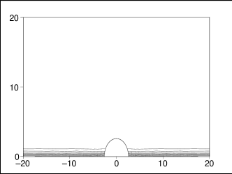
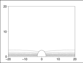
Figure 4: $X$ and $P$ Contours ($X$ and $P$ increase from $0.1$ to $0.9$ upward and downward respectively) for $l=1$ and $N=1$.

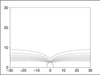
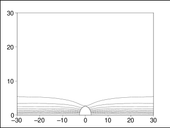
Figure 6: $X$ and $P$ Contours ($X$ and $P$ increase from $0.1$ to $0.9$ upward and downward respectively) for $l=1$ and $N=100$.

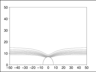
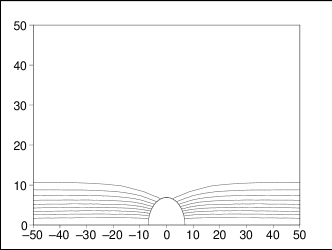
Figure 10: $X$ and $P$ Contours ($X$ and $P$ increase from $0.1$ to $0.9$ upward and downward respectively) for $l=5$ and $N=100$.

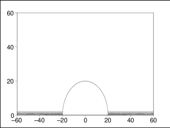
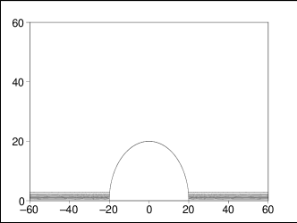
Figure 12: $X$ and $P$ Contours ($X$ and $P$ increase from $0.1$ to $0.9$ upward and downward respectively) for $l\rightarrow\infty$ and $N=1$.

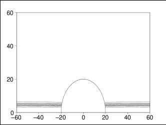
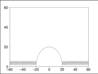
Figure 13: $X$ and $P$ Contours ($X$ and $P$ increase from $0.1$ to $0.9$ upward and downward respectively) for $l\rightarrow\infty$ and $N=10$.

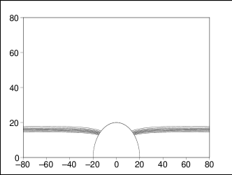
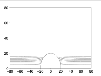
Figure 14: $X$ and $P$ Contours ($X$ and $P$ increase from $0.1$ to $0.9$ upward and downward respectively) for $l\rightarrow\infty$ and $N=100$.

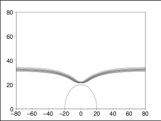
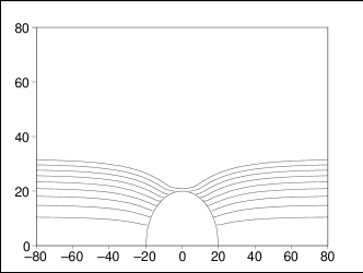
Figure 15: $X$ and $P$ Contours ($X$ and $P$ increase from $0.1$ to $0.9$ upward and downward respectively) for $l\rightarrow\infty$ and $N=400$.

The results of this calculation are displayed in figures (4) to ( 15) for different values of $l=1,5$ and $l\rightarrow\infty$  and winding numbers $N=1,10,100,400.$ In all of these figures, the black hole mass is taken have the constant value $m=10.$ Note that for $l\rightarrow\infty$ figures (12-15) are the same as the figures introduced in [5] for the Abelian-Higgs model in the flat spacetime. Like the flat spacetime case, in the AdS spacetime, increasing the winding number yields a greater vortex thickness. Comparing  figures (6,10 and 15) we see that as $l$ decreases the black hole is completely covered by a vortex of decreasingly large winding number. For example, for $l=1$ the black hole horizon is completely inside the core of a vortex with a winding numberof less than one hundred, but for $l\rightarrow\infty,$ this occurs for winding number about four hundred.

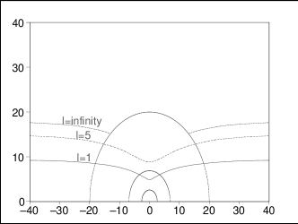
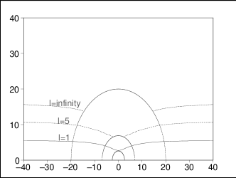
Figure 16: $X=0.9$ and $P=0.1$ Contours for $l=1$ (solid)$,5$ (dotted) and $l\rightarrow\infty$ (dashed) with winding number $N=100$.

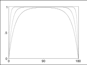
Figure 17: $X$ and $P$ fields on the horizon versus $\theta$ for $l=1$ (solid)$,5$ (dotted) and $l\rightarrow\infty$ (dashed) with winding number $N=1.$

Also, as figure (16) shows, for a string with definite winding number, the string core increases with increasing $l,$ but the ratio of string core to the black hole horizon decreases. Alternatively from figure (17) we see the $X$  and $P$ fields more rapidly approach their respective maximum and minimum values in smaller angle as $l$ increases.

4 Vortex Self Gravity on the AdS-Schwarzschild Black hole

We now consider the effect of  the vortex on the AdS-Schwarzschild black hole. As we have seen in section (2), this is a formidable problem even for flat or AdS spacetimes.

As in section (2), we assume that the thickness of string is much smaller that all the other relevant length scales and the gravitational effects of the string are weak enough so that the linearized Einstein-Abelian Higgs differential equations are applicable. So, we condsider thin string  with the winding number $N=1$ in the AdS-Schwarzschild background with $l=1$. The rescaled components of the energy-momentum tensor are

$$T_{tt}=(1-\frac{2m}{r}+\frac{r^{2}}{l^{2}})\{\frac{1}{2}(1-\frac{2m}{r}+\frac{r^{2}}{l^{2}})[(\frac{\partial X}{\partial r})^{2}+\frac{1}{\alpha r^{2}\sin^{2}\theta}(\frac{\partial P}{\partial r})^{2}]+\frac{1}{2r^{2}}(\frac{\partial X}{\partial\theta})^{2}+\frac{1}{2\alpha r^{4}\sin^{2}\theta}(\frac{\partial P}{\partial\theta})^{2}$$

(26)

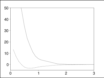
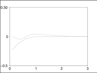
Figure 18: $T_{tt}$ (solid), $T_{\theta\theta}$ (dashed), $T_{\varphi\varphi}$ (dotted) and $T_{rr}$ (dot-dashed) curves versus $\rho$ in $\ z=5$ for the AdS-Schwarzschild black hole with $l=1$ and winding number $N=1.$

In the figures (18), the behaviour of the energy-momentum tensor components in a fixed $z$ is shown. The behaviour of the components in the other $z$ is like the same as these figures. As it is clear from figures, the components of the energy-momentunm tensor rapidly go to zero outside the core string, so the situation is like what happened in the pure AdS spacetime. Then performing the same calculation as in the pure AdS spacetime described in detail in section (2), give us the following metric of the AdS-Schwarzschild spacetime incorporated the effect of the vortex on it,

$$ds^{2}=-(1-\frac{2m}{r}+\frac{r^{2}}{l^{2}})dt^{2}+\frac{dr^{2}}{1-\frac{2m}{r}+\frac{r^{2}}{l^{2}}}+r^{2}(d\theta^{2}+\beta^{2}\sin^{2}\theta d\phi^{2})$$ (27)

The above metric describes an AdS-Schwarzschild metric with a deficit angle. So, using a physical Lagrangian based model, we have established that the presence of the cosmic string induces a deficit angle in the black hole metric.

5 Polystring Configuration

From the precceding sections we know that an AdS-Schwarzschild  black hole could support a long range Nielsen-Olesen vortex string as stable hair. The natural next question is, how many strings could be supported by such a black hole?

Such a question was considered for the Schwarzschild black hole.  In [19], a three string configuration in Schwarzscild black hole was studied. Also, in [6], all possible multistring configurations were presented.

Since the intersection of strings with the AdS-Schwarzschild black hole occurs on some points on the horizon which is topologically $S^{2},$ and such a situation also holds for the Schwarzschild black hole whose horizon has spherical topology, we could use the same procedure as was presented in [6]. So, we give an argument in brief to show the different possible multistring-AdS Schwarzschild black hole system.

We assume strings enter the horizon along radii. The different polystring configurations are obtained by demanding that the black hole-multistring system must be invariant under any rotation about any axis which coincides with the strings. This condition is necessary since the black hole-multistring system must be in force-free equilibrium. The intersection of strings with the black hole occur on some points on the horizon which is topologically $S^{2},$ and these points are the vertexes of a spherical tesselation. The spherical tesselation is obtained by projection of the edges of a polyhedron from its geometrical center onto a concentric sphere. Every edge and vertex of the polyhedron is mapped to an arc of a great circle on the sphere and a vertex of spherical tesselation respectively. The spherical tesselation is invariant under a discrete rotation group. The elements of this discrete group are just rotation around every axis which passes through the center of the sphere and vertices, mid-arc points and centers of  faces of  spherical tesselation, respectively. This discrete rotation group of the spherical tesselation is in correspondence with the rotational symmetry group of the polyhedron. So the black hole-polystring system with radial strings is invariant under discrete rotations and hence is in an equilibrium state.

By knowing the properties of spherical tesselation, in [6], the different multistring configurations are introduced. The first configuration is 14 strings which are pierced to the black hole on the symmetry axis of a tetrahedron. The second and third configurations are 26 and 62 strings which are pierced to the black hole on the symmetry axis of a octahedron and icosahedron respectively. The fourth configuration is 2N strings (N is any arbitrary number) which corresponds to the symmetry axis of a double pyramid.

6 Conclusion

The effect of a vortex on pure AdS spacetime to create a deficit angle in the metric in the thin vortex approximation. We have extended this result, establishing numerically that Abelian Higgs vortices of finite thickness can pierce an AdS-Schwarzschild black hole horizon. These solutions could thus be interpreted as stable Abelian hair for the black hole. We have obtained numerical solutions for various cosmological constants and string winding numbers. Our solutions in the limit of  $l\rightarrow\infty,$ coincides with the known solutions in the asymptotically flat spacetime.

We found that by increasing the winding number, the string core increases. Also, the generalization to include piercing of more strings to the black hole has been considered and it is shown that there are four different polystring configurations. Finally, inclusion of the self gravity of the vortex in the AdS-Schwarzschild background metric was shown to induce a deficit angle in the AdS-Schwarzschild metric.

Other related problems such as study of the vortex in the charged or rotating black hole backgrounds and non-abelian vortex solution in asymtotically AdS spacetime remain to be carried out. Another issue is the holographic description of vortex solution in these asymptotically AdS spacetimes. Work on these problems is in progress.

Acknowledgments

This work was supported by the Natural Sciences and Engineering Research Council of Canada.

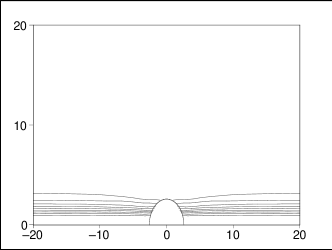
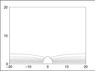
Figure 5: $X$ and $P$ Contours ($X$ and $P$ increase from $0.1$ to $0.9$ upward and downward respectively) for $l=1$ and $N=10$.

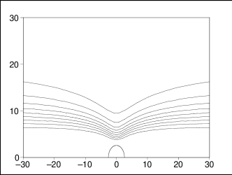
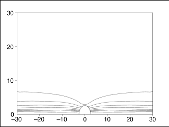
Figure 7: $X$ and $P$ Contours ($X$ and $P$ increase from $0.1$ to $0.9$ upward and downward respectively) for $l=1$ and $N=400$.

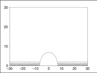
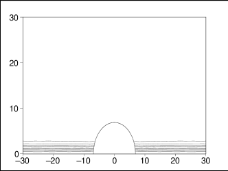
Figure 8: $X$ and $P$ Contours ($X$ and $P$ increase from $0.1$ to $0.9$ upward and downward respectively) for $l=5$ and $N=1$.

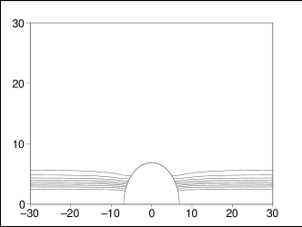
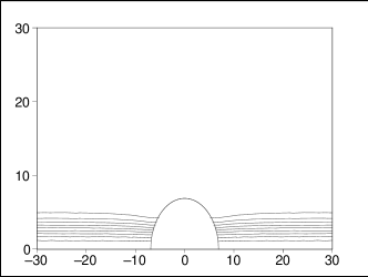
Figure 9: $X$ and $P$ Contours ($X$ and $P$ increase from $0.1$ to $0.9$ upward and downward respectively) for $l=5$ and $N=10$.

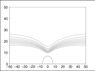
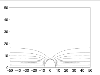
Figure 11: $X$ and $P$ Contours ($X$ and $P$ increase from $0.1$ to $0.9$ upward and downward respectively) for $l=5$ and $N=400$.

References

• [1] R. Ruffini and J.A. Wheeler. Phys. Today 24, 30 (1971).
• [2] D. Sudarsky, Class. Quant. Grav. 12, 579 (1995).
• [3] T. Torii, K. Maeda and M. Narita, Phys. Rev. D59, 064027 (1999).
• [4] E. Winstanley, Class. Quant. Grav. 16, 1963 (1999).
• [5] A. Achucarro, R. Gregory, K. Kuijken, Phys. Rev. Β D52, 5729 (1995)
• [6] V. Frolov and D. Fursaev, Class. Quant. Grav. Β 18, 1535 (2001).
• [7] J. Maldacena, Adv. Theor. Math. Phys. 2, 231 (1998).
• [8] E. Witten, Adv. Theor. Math. Phys. 2, 253 (1998).
• [9] M.H. Dehghani, A.M. Ghezelbash and R.B. Mann, hep-th/0105134.
• [10] T. Torii, K. Maeda and M. Narita, Phys. Rev. D64, 044007 (2001).
• [11] V. Balasubramanian, P. Kraus, A. Lawrence and S.P. Trivedi, Phys. Rev. D59, 104021 (1999).
• [12] U.H. Danielsson, E. Keski-Vakkuri and M. Kruczenski, JHEP 01, 002 (1999).
• [13] V. Balasubramanian and S.F. Ross, Phys. Rev. D61, 044007 (2000).
• [14] H.B. Nielsen and P.Olesen, Nucl. Phys. B61, 45 (1973).
• [15] J. L. Synge, ”Relativity: The General Theory”, Amsterdam: North Holland (1960).
• [16] R.B. Mann, Phys. Rev. D60, 104047 (1999); R. Emparan, C.V. Johnson and R. Meyers, Phys. Rev. D60, 104001 (1999); M. Hennigson and K. Skenderis, JHEP 9807023 (1998) ;Β Β S.Y. Hyun, W.T. Kim and J. Lee, Phys. Rev. D59 084020 (1999) ;Β Β V. Balasubramanian and P. Kraus, Commun. Math. Phys. 208, 413 (1999).
• [17] J.D. Brown, J. Creighton and R.B. Mann, Phys. Rev. D50, 6394 (1994).
• [18] W. H. Press, S. A. Teukolsky, W. T. Vetterling and B. P. Flannery, ”Numerical Recipes in FORTRAN”, Cambridge University Press (1992).
• [19] J. S. Dowker and P. Chang, Phys. Rev. D46, 3458 (1992).
Refer to caption
Refer to caption