UT-950 KEK Preprint 2001-53 hep-th/0107217
Stability of Quiver Representations
and Topology Change

Abstract

We study phase structure of the moduli space of a D0-brane on the orbifold ${\bf C}^{3}/{\bf Z}_{2}\times{\bf Z}_{2}$ based on stability of quiver representations. It is known from an analysis using toric geometry that this model has multiple phases connected by flop transitions. By comparing the results of the two methods, we obtain a correspondence between quiver representations and geometry of toric resolutions of the orbifold. It is shown that a redundancy of coordinates arising in the toric description of the D-brane moduli space, which is a key ingredient of disappearance of non-geometric phases, is understood from the monodromy around the orbifold point. We also discuss why only geometric phases appear from the viewpoint of stability of D0-branes.

1 Introduction

D-branes allow us to study the structure of geometry at sub-stringy scales. From this perspective, space-time is a derived concept appearing as a vacuum moduli space of the D-brane worldvolume gauge theory. A number of works have been devoted to investigating geometry as seen by D-branes and comparing it with standard classical geometry or geometry probed by fundamental strings.

In [1], it was pointed out that D-branes on orbifolds ${\bf C}^{2}/\Gamma$ are described by quiver gauge theories, where a quiver is a diagram representing algebraic structure of the group $\Gamma$. It implies that D-branes give a physical explanation of the McKay correspondence: a relation between geometry of resolutions of an orbifold ${\bf C}^{n}/\Gamma$ and the representation theory of $\Gamma$. (For mathematics on the McKay correspondence, see [2]-[5].) The purpose of this paper is to study a relation between geometry of an orbifold ${\bf C}^{n}/\Gamma$ probed by a D0-brane and the representation theory of $\Gamma$ based on the concept of stability of the D0-brane.

Stability has been recently brought to attention as it plays an important role in studying D-branes on Calabi-Yau manifolds [6]-[10]. The relevant notion of stability near the orbifold point in the K${\rm{\ddot{a}}}$hler moduli space is $\theta$-stability of representations of quivers [11]. It enables us to construct the vacuum moduli space of the quiver gauge theories without solving all equations defining the vacua and to study the marginal stability loci, where D-brane spectrum jumps.

We would like to compare the results obtained from stability of quiver representations corresponding to a D0-brane with geometric structure of three-dimensional orbifolds ${\bf C}^{3}/\Gamma$ with $\Gamma$ an abelian subgroup of $SU(3)$. The latter is investigated following the procedure given in [12]. In this formulation, the vacuum moduli space is obtained by solving both F-flatness and D-flatness conditions, the equations defining the vacua, with the aid of toric geometry. The D-flatness conditions contain Fayet-Iliopoulos terms originating from twisted sectors of closed strings, which parameterize the K${\rm{\ddot{a}}}$hler moduli space of the orbifold. The core of the method in [12] is to convert F-flatness conditions into D-flatness conditions of an auxiliary gauge theory with a large number of chiral multiplets. Scalar components of the chiral multiplets become homogeneous coordinates describing the vacuum moduli space. After reducing redundant coordinates by using D-flatness conditions and gauge symmetry, we obtain the vacuum moduli space of the quiver gauge theory.

Various models were investigated following this procedure [13]-[17]. The most striking feature common to these analyses is that non-geometric phases are projected out. This is in contrast to the analyses based on fundamental strings [18, 19], in which non-geometric phases are realized as abstract conformal field theories. By inspecting the process of the calculation of the D-brane moduli spaces, we can see that the key to the disappearance of non-geometric phases is the redundancy of coordinates mentioned above. So far, however, physical origin of the redundancy has not been clarified; it just arises as a result of a combinatorial algorithm converting F-flatness conditions to D-flatness conditions. To understand this point is one motivation of this work.

The orbifold we study in this paper is ${\bf C}^{3}/{\bf Z}_{2}\times{\bf Z}_{2}$. A reason to study this orbifold is that it has a rather rich structure in spite of its simplicity; it contains multiple phases that are related by topology changing processes called flops [14, 15] as we review in section 2. We also see that non-geometric phases disappear due to the redundancy of homogeneous coordinates. In section 3 we re-examine the moduli space of D0-branes based on $\theta$-stability of quiver representations. By comparing the results with those obtained in section 2, we obtain a correspondence between homology cycles of a resolution of the orbifold and quiver representations. Furthermore, we find that the redundancy of the homogeneous coordinates stems from monodromy around the orbifold point in the K${\rm{\ddot{a}}}$hler moduli space. Finally, we discuss the disappearance of non-geometric phases from the viewpoint of stability of D0-branes.

2 D-branes on ${\bf C}^{3}/{\bf Z}^{2}\times{\bf Z}^{2}$: an analysis based on toric geometry

In this section, we first review the method given in [12] to study D0-branes on orbifolds ${\bf C}^{3}/\Gamma$ with $\Gamma\in SU(3)$. Second, we present the geometric structure of the orbifold ${\bf C}^{3}/{\bf Z}^{2}\times{\bf Z}^{2}$ obtained by this method [14, 15].

D-branes on orbifolds ${\bf C}^{3}/\Gamma$ are described by quiver gauge theories. A quiver is a graph consisting of a set of nodes $v_{i}\in V$ and a set of arrows $a_{ij}\in A$ starting from the node $v_{i}$ and ending at the node $v_{j}$. We will denote the number of the nodes as $N$. Given a quiver, one obtains a gauge theory by considering a representation of the quiver. A representation $R$ of a quiver is a collection of finite dimensional vector spaces $V_{i}$, one for each node $v_{i}\in V$, and a collection of linear maps $X_{ij}:V_{i}\rightarrow V_{j}$, one for each arrow $a_{ij}\in A$. The vector $(n_{0},n_{1},...,n_{N-1})$, where $n_{i}$ is the dimension of the vector space $V_{i}$, is referred to as the dimension vector of the representation $R$.

The gauge theory corresponding to a representation $R$ is an ${\cal N}=1$ supersymmetric gauge theory with a gauge symmetry $G=\Pi_{v_{i}\in V}U(n_{i})/U(1)$: a node $v_{i}$ represents a factor of $U(n_{i})$ in the gauge group $G$, and an arrow $a_{ij}$ represents a chiral multiplet transforming as $(n_{i},{\bar{n}_{j}})$ under $U(n_{i})\times U(n_{j})$. Note that the factor $U(1)$ in the gauge group is the diagonal subgroup of $\Pi_{v_{i}\in V}U(n_{i})$ which acts trivially.

A quiver relevant to the discussion of D-branes on ${\bf C}^{3}/\Gamma$ is the McKay quiver associated to $\Gamma$. Nodes in the McKay quiver correspond to irreducible representations of $\Gamma$, and arrows encode information on tensor products of a three-dimensional representation defining the action of $\Gamma$ on ${\bf C}^{3}$ and irreducible representations of $\Gamma$. In this paper, we restrict $\Gamma$ to be an abelian subgroup of $SU(3)$, whose irreducible representations are one-dimensional. In that case, the number $N$ of nodes in the McKay quiver coincides with the order of $\Gamma$. Thus a D0-brane on an orbifold ${\bf C}^{3}/\Gamma$, which we would like to discuss, corresponds to a quiver representations with a dimension vector $(1,1,...,1)$.

We are concerned with the vacuum moduli space $\cal M$ of the quiver gauge theory. The vacua are parameterized by values for scalars in the chiral multiplets, modulo gauge equivalence, solving F-flatness and D-flatness conditions. In [12], it was found to be convenient to consider F-flatness conditions as if they were D-flatness conditions in an auxiliary gauge theory. The vacuum moduli space of this auxiliary gauge theory is a $(N+2)$-dimensional space of the following form,

$$\{(p_{1},...p_{c})\in{\bf C}^{c}|(c-N-2)\;\mbox{D-flatness conditions}\}/U(1)^{c-N-2},$$ (2.1)

where $c$ is the number of scalars in the chiral multiplets of the auxiliary gauge theory. The data necessary to construct this space are obtained through a combinatorial algorithm based on toric geometry. This process is burdensome in general, and hence an analytic expression of $c$ is not known for ${\bf C}^{3}/{\bf Z}_{n}$ nor ${\bf C}^{3}/{\bf Z}_{n}\times{\bf Z}_{m}$.

To obtain the vacuum moduli space ${\cal M}$ of the quiver gauge theory, one must further impose D-flatness conditions

$$D_{i}=\sum_{j}(X_{ji}^{\dagger}X_{ji}-X_{ij}X_{ij}^{\dagger})=\theta_{i},$$ (2.2)

that exist in the quiver gauge theory from the beginning. Note that although the index $i$ takes values from 0 to $N-1$, the number of independent conditions is $N-1$. Real parameters $\theta_{i}$ come from twisted sectors of NS-NS fields, and they are related to physical Fayet-Iliopoulos parameters $\zeta_{i}$ through the following relation:

$$\theta_{i}=\zeta_{i}-\frac{\sum_{k}\zeta_{k}n_{k}}{\sum_{l}n_{l}}.$$ (2.3)

This relation comes from the requirement of quasi-supersymmetry of the vacuum [6]. In the case of $(n_{0},n_{1},...,n_{N-1})=(1,1,...,1)$, $\theta_{i}$ coincide with the physical Fayet-Iliopoulos parameters $\zeta_{i}$.

The total number of D-flatness conditions to be imposed on the auxiliary gauge theory is $(c-N-2)+(N-1)=c-3$, and gauge symmetry is $U(1)^{c-N-2}\times U(1)^{N-1}=U(1)^{c-3}$. Thus the moduli space $\cal M$ takes the form

$${\cal M}=\{(p_{1},...,p_{c})\in{\bf C}^{c}|(c-3)\;\mbox{D-flatness conditions}\}/U(1)^{c-3}.$$ (2.4)

Note that the $N-1$ D-flatness conditions in equation (2.2) have Fayet-Iliopoulos parameters $\theta_{i}$, while $c-N-2$ D-flatness conditions coming from F-flatness conditions do not have such parameters.

Now we investigate the case ${\bf C}^{3}/{\bf Z}_{2}\times{\bf Z}_{2}$ in detail [14, 15]. Non-trivial elements $g_{1},g_{2}$ $g_{3}$ of $\Gamma={\bf Z}_{2}\times{\bf Z}_{2}$ act on the coordinates $(z_{1},z_{2},z_{3})$ of ${\bf C}^{3}$ as follows:

$$g_{1}:(z_{1},z_{2},z_{3})\rightarrow(z_{1},-z_{2},-z_{3}),$$

$$g_{2}:(z_{1},z_{2},z_{3})\rightarrow(-z_{1},z_{2},-z_{3}),$$ (2.5)

$$g_{3}:(z_{1},z_{2},z_{3})\rightarrow(-z_{1},-z_{2},z_{3}).$$

Here $g_{1}^{2}=g_{2}^{2}=g_{3}^{2}=1,~{}g_{1}g_{2}=g_{3}$. Since ${\bf Z}_{2}\times{\bf Z}_{2}$ is an abelian group of order four, there are four irreducible representations with dimension one. The quiver diagram is depicted in Figure 1.

Figure 1: The quiver diagram for ${\bf Z}_{2}\times{\bf Z}_{2}$.

Since the quiver has four nodes ($N=4$), the associated quiver gauge theory has a gauge symmetry $U(1)^{3}$ and three Fayet-Iliopoulos parameters $\theta_{i}$. The vacuum moduli space of the quiver gauge theory is computed following the procedure stated above. In this case, the combinatorial algorithm gives an auxiliary gauge theory with $c=9$. Therefore the vacuum moduli space ${\cal M}$ is represented as,

$${\cal M}=\{(p_{1},...p_{9})\in{\bf C}^{9}|6\;\mbox{D-flatness conditions}\}/U(1)^{6},$$ (2.6)

where six D-flatness conditions are

$$-|p_{4}|^{2}+|p_{7}|^{2} = 2\tilde{\theta}_{1},$$ (2.7)

$$-|p_{5}|^{2}+|p_{8}|^{2} = 2\tilde{\theta}_{2},$$ (2.8)

$$-|p_{6}|^{2}+|p_{9}|^{2} = 2\tilde{\theta}_{3},$$ (2.9)

$$|p_{1}|^{2}+|p_{4}|^{2}-|p_{5}|^{2}-|p_{6}|^{2} = -\tilde{\theta}_{1}+\tilde{\theta}_{2}+\tilde{\theta}_{3},$$ (2.10)

$$|p_{2}|^{2}-|p_{4}|^{2}+|p_{5}|^{2}-|p_{6}|^{2} = \tilde{\theta}_{1}-\tilde{\theta}_{2}+\tilde{\theta}_{3},$$ (2.11)

$$|p_{3}|^{2}-|p_{4}|^{2}-|p_{5}|^{2}+|p_{6}|^{2} = \tilde{\theta}_{1}+\tilde{\theta}_{2}-\tilde{\theta}_{3}.$$ (2.12)

Here we have used parameters $\tilde{\theta}_{1}=(\theta_{2}+\theta_{3})/2,~{}\tilde{\theta}_{2}=(\theta_{3}+\theta_{1})/2,~{}\tilde{\theta}_{3}=(\theta_{1}+\theta_{2})/2$.

We first study the geometric structure of $\cal M$ in the region $\tilde{\theta}_{1}>0$, $\tilde{\theta}_{2}>0$, $\tilde{\theta}_{3}>0$. For $\tilde{\theta}_{1}>0$, $p_{7}$ is nonzero due to the equation (2.7). Combining with a U(1) gauge symmetry corresponding to this D-flatness condition, we can eliminate $p_{7}$. Similarly, in the region $\tilde{\theta}_{2}>0$ ($\tilde{\theta}_{3}>0$), we can eliminate $p_{8}$ (respectively $p_{9}$). Thus in the region $\tilde{\theta}_{1}>0$, $\tilde{\theta}_{2}>0$ and $\tilde{\theta}_{3}>0$, the six D-flatness conditions are reduced to the last three equations (2.10), (2.11), (2.12). They describe a resolution of ${\bf C}^{3}/{\bf Z}_{2}\times{\bf Z}_{2}$. However, the topology of the resolution is not fixed uniquely since the inequalities $\tilde{\theta}_{1}>0$, $\tilde{\theta}_{2}>0$, $\tilde{\theta}_{3}>0$ do not fix the sign of the right-hand side of (2.10), (2.11), (2.12); flop transition occurs as the sign of the right-hand side changes. For example, in the region $\theta_{1}=-\tilde{\theta}_{1}+\tilde{\theta}_{2}+\tilde{\theta}_{3}>0,~{}\theta_{2}=\tilde{\theta}_{1}-\tilde{\theta}_{2}+\tilde{\theta}_{3}>0,~{}\theta_{3}=\tilde{\theta}_{1}+\tilde{\theta}_{2}-\tilde{\theta}_{3}>0$, the resolved orbifold has a topology represented by the toric diagram drawn in Figure 2(a). Each line in the diagram represents homology 2-cycle $C_{i}$ in the resolution of ${\bf C}^{3}/{\bf Z}_{2}\times{\bf Z}_{2}$, whose volume is parameterized by $\theta_{i}$. If we change the sign of $\theta_{1}$, $C_{1}$ is replaced by $C^{\prime}_{1}$ as depicted in Figure 2(b). The volume of $C^{\prime}_{1}$ is parameterized by $-\theta_{1}$, which implies that the homology class $[C^{\prime}_{1}]$ is equal to $-[C_{1}]$ as noted in [20].

Figure 2: Toric diagrams representing the topology of the resolved orbifold (a) in the region $\theta_{1}>0,~{}\theta_{2}>0,~{}\theta_{3}>0$, and (b) in the region $\theta_{1}<0,~{}\tilde{\theta}_{2}=(\theta_{1}+\theta_{3})/2>0,~{}\tilde{\theta}_{3}=(\theta_{1}+\theta_{2})/2>0$.

Before we come to the analysis outside of $\tilde{\theta}_{1}>0,~{}\tilde{\theta}_{2}>0,~{}\tilde{\theta}_{3}>0$, we comment on the phase structure obtained from just the three D-flatness conditions (2.10), (2.11), (2.12). These are the D-flatness conditions that appear in the analysis of the orbifold ${\bf C}^{3}/{\bf Z}_{2}\times{\bf Z}_{2}$ based on fundamental strings [19]. In the region $\tilde{\theta}_{1}>0,~{}\tilde{\theta}_{2}>0,~{}\tilde{\theta}_{3}>0$, one obtains the same resolutions of the orbifold as described above. In another region, however, one obtains a singular space. Such regions are called non-geometric phases realized as abstract conformal field theories.

Now we come back to the analysis of the six D-flatness conditions from (2.7) to (2.12). If we consider the region $\tilde{\theta}_{2}<0$ instead of $\tilde{\theta}_{2}>0$, we can eliminate $p_{5}$ instead of $p_{8}$ by using the D-flatness condition (2.8). In this case, we obtain the following three D-flatness conditions.

$$|p_{1}|^{2}+|p_{4}|^{2}-|p_{8}|^{2}-|p_{6}|^{2} = -\tilde{\theta}_{1}+(-\tilde{\theta}_{2})+\tilde{\theta}_{3},$$ (2.13)

$$|p_{2}|^{2}-|p_{4}|^{2}+|p_{8}|^{2}-|p_{6}|^{2} = \tilde{\theta}_{1}-(-\tilde{\theta}_{2})+\tilde{\theta}_{3},$$ (2.14)

$$|p_{3}|^{2}-|p_{4}|^{2}-|p_{8}|^{2}+|p_{6}|^{2} = \tilde{\theta}_{1}+(-\tilde{\theta}_{2})-\tilde{\theta}_{3}.$$ (2.15)

One can see that the equations (2.13), (2.14), (2.15) have the same structure as the equations (2.10), (2.11), (2.12) if we take into account that we are considering the region $\tilde{\theta}_{2}<0$ instead of $\tilde{\theta}_{2}>0$. Therefore, phase structure in this region is the same as that in the region $\tilde{\theta}_{1}>0$, $\tilde{\theta}_{2}>0$ and $\tilde{\theta}_{3}>0$. In this way, we obtain phase structure near the orbifold point in the K${\rm{\ddot{a}}}$hler moduli space as shown in Figure 3. With eight ($=2^{3}$) ways of eliminating the coordinates mentioned above, there are 32 phases in all.

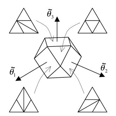
Figure 3: The phase structure of the orbifold ${\bf C}^{3}/{\bf Z}_{2}\times{\bf Z}_{2}$ probed by a D0-brane near the orbifold point of the K${\rm{\ddot{a}}}$hler moduli space. Each toric diagram represents topology of the resolution of ${\bf C}^{3}/{\bf Z}_{2}\times{\bf Z}_{2}$ in each phase.

The most striking feature of the result is that non-geometric phases do not appear in contrast to the analyses based on fundamental strings. We can see that what makes non-geometric phases disappear is the redundancy of the homogeneous coordinates $p_{a}$. At each point in the K${\rm{\ddot{a}}}$hler moduli space, we need only six coordinates out of nine to describe $\cal M$, but which coordinates we should choose depends on the region in the K${\rm{\ddot{a}}}$hler moduli space as stated above. Thus it is important to clarify the physical origin of the redundancy of the coordinates to understand the reason that D-branes avoid non-geometric phases.

3 D-branes on ${\bf C}^{3}/{\bf Z}^{2}\times{\bf Z}^{2}$: an analysis based on $\theta$-stability

In section 2, we have studied the vacuum moduli space of the worldvolume gauge theory of a D0-brane on the orbifold ${\bf C}^{3}/{\bf Z}^{2}\times{\bf Z}^{2}$ based on the method using toric geometry. In this section, we re-examine the same space by using $\theta$-stability of quiver representations.

The reformulation arises as follows. First, consider the space of solutions of F-flatness conditions. Since it is invariant under the action of the complexified gauge group $G_{\bf C}$, one can talk about the $G_{\bf C}$-orbits satisfying the F-flatness conditions. The key point is that, under certain conditions, the $G_{\bf C}$-orbit satisfying the F-flatness conditions contains a solution of D-flatness conditions. They are $\theta$-stability conditions of quiver representations [11].

To study $\theta$-stability of a quiver representation we need to know its subrepresentations. A representation $R^{\prime}$ is a subrepresentation of $R$ if there is an injective homomorphism from $R^{\prime}$ to $R$. Here a homomorphism between two representations $R=\{V_{i},X_{ij}\}$ and $R^{\prime}=\{V^{\prime}_{i},X^{\prime}_{ij}\}$ is a collection of linear maps $\phi_{i}:V^{\prime}_{i}\rightarrow V_{i}$ which satisfy $\phi_{i}X_{ij}=X^{\prime}_{ij}\phi_{j}$ as matrices. A quiver representation with a dimension vector $n$ is $\theta$-semistable if it satisfies

$$\sum n_{i}\theta_{i}=0,$$ (3.1)

and every subrepresentation with a dimension vector $n^{\prime}$ satisfies

$$\sum n^{\prime}_{i}\theta_{i}\geq 0.$$ (3.2)

Furthermore, a representation is $\theta$-stable if every non-trivial subrepresentations satisfies $\sum n^{\prime}_{i}\theta_{i}>0$. Note that the equation (3.1) follows by taking traces of the D-flatness conditions (2.2), so the parameters $\theta_{i}$ in the expression coincide with the parameters appearing in the D-flatness conditions.

To find out $\theta$-stable representations, it is useful to consider Schur representations. A representation $R$ is Schur if it satisfies End$R={\bf C}$. This condition implies that Schur representations correspond to D-brane bound states [7]. Since $\theta$-stable representations are Schur, we obtain $\theta$-stable representations by considering Schur representations which satisfy F-flatness conditions, and then imposing $\theta$-stability conditions on the Schur representations.

In the case of ${\bf C}^{3}/{\bf Z}_{2}\times{\bf Z}_{2}$, endomorphism of a representation with a dimension vector $(1,1,1,1)$ consists of four linear maps $\lambda_{i}:V_{i}\rightarrow V_{i}$. The condition for the representation to be Schur is that the equations $\lambda_{i}X_{ij}=X_{ij}\lambda_{j}$ for $i\neq j$ have a unique solution $\lambda_{1}=\lambda_{2}=\lambda_{3}=\lambda_{4}=\lambda\in{\bf C}$. It requires that all the nodes in the quiver diagram must be connected by arrows corresponding to non-vanishing $X_{ij}$’s. Under this condition, we fix three $X_{ij}$’s to be zero by using the complexified gauge symmetry $G_{\rm C}=GL(3,{\bf C})$. Since we also impose F-flatness conditions $X_{ik}X_{kj}=X_{il}X_{lj}$ with $k\neq l$, more than three $X_{ij}$’s vanish in general. The least number of non-vanishing $X_{ij}$’s is three, which corresponds to the dimension of the orbifold. To be consistent with the F-flatness conditions, any neighboring two arrows out of the three are in opposite directions. By examining the conditions in detail, we found that there are 32 Schur representations with three non-vanishing $X_{ij}$’s. We will illustrate these representations by eliminating arrows corresponding to vanishing $X_{ij}$’s from the quiver diagram. The 32 Schur representations are classified into three types according to their forms as graphs.

Figure 4: Schur representations with a dimension vector $(1,1,1,1)$. Arrows from $v_{i}$ to $v_{j}$ represent non-vanishing $X_{ij}$’s. (a) The first type of Schur representations. Three arrows start from one node. (b) The second type of Schur representations. Three arrows end at one node. (c)(d) The third type of Schur representations. Three arrows connecting four nodes form a line.

The first type of Schur representations are such that three arrows start from one node as shown in Figure 4(a). By exchanging labels of nodes, we obtain four Schur representations of this type. The Schur representation in Figure 4(a) has seven subrepresentations with the following dimension vectors,

$$(0,1,1,1),(0,0,1,1),(0,1,0,1),(0,1,1,0),(0,1,0,0),(0,0,1,0),(0,0,0,1),$$ (3.3)

which are determined by the condition that an injective homomorphism exists: when $X_{ij}$ is non-vanishing, $n_{j}=0$ implies $n_{i}=0$. Hence $\theta$-stability of the representation requires

$$\theta_{1}+\theta_{2}+\theta_{3}>0,~{}\theta_{2}+\theta_{3}>0,~{}\theta_{3}+\theta_{1}>0,$$

$$\theta_{1}+\theta_{2}>0,~{}\theta_{1}>0,~{}\theta_{2}>0,~{}\theta_{3}>0.$$ (3.4)

Thus the representation in Figure 4(a) is $\theta$-stable in the region $\theta_{1}>0,~{}\theta_{2}>0,~{}\theta_{3}>0$. They are rewritten as $\tilde{\theta}_{2}+\tilde{\theta}_{3}>0,~{}\tilde{\theta}_{3}+\tilde{\theta}_{1}>0,~{}\tilde{\theta}_{1}+\tilde{\theta}_{2}>0$.

The second type of Schur representations are such that three arrows end at one node as shown in Figure 4(b). There are four Schur representations of this type. The representation in Figure 4(b) has seven subrepresentations,

$$(1,0,0,0),(1,1,0,0),(1,0,1,0),(1,0,0,1),(1,0,1,1),(1,1,0,1),(1,1,1,0),$$ (3.5)

and hence $\theta$-stability of the representation requires

$$\theta_{1}+\theta_{2}+\theta_{3}<0,~{}\theta_{1}+\theta_{2}<0,~{}\theta_{1}+\theta_{3}<0,$$

$$\theta_{2}+\theta_{3}<0,~{}\theta_{1}<0,~{}\theta_{2}<0,~{}\theta_{3}<0,$$ (3.6)

where we have used $\theta_{0}+\theta_{1}+\theta_{2}+\theta_{3}=0$. Thus the representation in Figure 4(b) is $\theta$-stable in the region $\theta_{1}<0,~{}\theta_{2}<0,~{}\theta_{3}<0$ ($\tilde{\theta}_{2}+\tilde{\theta}_{3}<0,~{}\tilde{\theta}_{3}+\tilde{\theta}_{1}<0,~{}\tilde{\theta}_{1}+\tilde{\theta}_{2}<0$).

The third type of Schur representations are such that three arrows connecting four nodes form a line as shown in Figure 4(c) and 4(d). Permutation of labels of nodes gives 24 representations of this type. The representation in Figure 4(c) has six subrepresentations,

$$(0,1,1,1),(0,0,1,1),(1,0,1,1),(0,0,1,0),(0,0,0,1),(0,1,1,0),$$ (3.7)

and hence $\theta$-stability of the representation requires

$$\theta_{1}+\theta_{2}+\theta_{3}>0,~{}\theta_{2}+\theta_{3}>0,$$

$$\theta_{1}<0,~{}\theta_{2}>0,~{}\theta_{3}>0,~{}\theta_{1}+\theta_{2}>0.$$ (3.8)

Thus the representation is $\theta$-stable in the region $\theta_{1}+\theta_{2}>0,~{}\theta_{1}<0,~{}\theta_{3}>0$ ($\tilde{\theta}_{3}>0,~{}-\tilde{\theta}_{1}+\tilde{\theta}_{2}+\tilde{\theta}_{3}<0,~{}\tilde{\theta}_{1}+\tilde{\theta}_{2}-\tilde{\theta}_{3}>0$). The Schur representation in Figure 4(d) also has six subrepresentations

$$(0,1,1,1),(0,0,1,1),(1,0,1,1),(0,0,1,0),(0,0,0,1),(0,1,0,1).$$ (3.9)

As one can see, the first five subrepresentations of (3.9) coincide with those of (3.7); the only differences between (3.7) and (3.9) are the last ones, $(0,1,1,0)$ and $(0,1,0,1)$. The representation in Figure 4(d) is $\theta$-stable in the region $\theta_{1}+\theta_{3}>0,~{}\theta_{1}<0,~{}\theta_{2}>0$ ($\tilde{\theta}_{2}>0,~{}-\tilde{\theta}_{1}+\tilde{\theta}_{2}+\tilde{\theta}_{3}<0,~{}\tilde{\theta}_{1}-\tilde{\theta}_{2}+\tilde{\theta}_{3}>0$).

In this way, we can study regions in which Schur representations are $\theta$-stable. We found that the $\theta$-stable regions for the 32 Schur representations cover the $\tilde{\theta}$-space except for codimension-one marginal stability loci. It was also found that a $\theta$-stable region for a Schur representation of the first or second type does not overlap with a $\theta$-stable region for another Schur representation. Thus in the region $\tilde{\theta}_{2}+\tilde{\theta}_{3}>0,~{}\tilde{\theta}_{3}+\tilde{\theta}_{1}>0,~{}\tilde{\theta}_{1}+\tilde{\theta}_{2}>0$, for example, the $\theta$-stable representation is the one in Figure 4(a), and there are seven subrepresentations (3.3).

In contrast, $\theta$-stable regions for Schur representations of the third type overlap with each other. For example, the two representations in Figures 4(c) and 4(d) have a common $\theta$-stable region, $\tilde{\theta}_{2}>0,~{}\tilde{\theta}_{3}>0$, $-\tilde{\theta}_{1}+\tilde{\theta}_{2}+\tilde{\theta}_{3}<0$. Therefore, a set of subrepresentations in this region is the union of (3.7) and (3.9):

$$(0,1,1,1),(0,0,1,1),(1,0,1,1),(0,0,1,0),(0,0,0,1),(0,1,1,0),(0,1,0,1).$$ (3.10)

In this way, we can investigate the structure of subrepresentations for any point in the $\tilde{\theta}$-space. We found that there are 32 phases in all, just as in section 2. In fact, there is a simple method to read off the structure of subrepresentations. First consider a cuboctahedron, a polyhedron with six squares and eight triangles obtained from a cube by truncating its eight apices. Next put it at the origin of the $\tilde{\theta}$-space in such a way that squares face to three axes $\tilde{\theta}_{1}$, $\tilde{\theta}_{2}$ and $\tilde{\theta}_{3}$. Then assign fourteen non-trivial subrepresentations of $(1,1,1,1)$ to fourteen surfaces of the cuboctahedron in the following way. Let us define $\tilde{n}_{1}=-n_{1}+n_{2}+n_{3},~{}\tilde{n}_{2}=n_{1}-n_{2}+n_{3},~{}\tilde{n}_{3}=n_{1}+n_{2}-n_{3}$. A subrepresentation $(0,n_{1},n_{2},n_{3})$ is assigned to the surface with a normal vector $(\tilde{n}_{1},\tilde{n}_{2},\tilde{n}_{3})$ and a subrepresentation $(1,1-n_{1},1-n_{2},1-n_{3})$ to the surface with a normal vector $(-\tilde{n}_{1},-\tilde{n}_{2},-\tilde{n}_{3})$. The assignment is drawn in Figure 5.

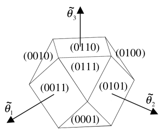
Figure 5: A cuboctahedron useful to read off the structure of subrepresentations. We assign fourteen non-trivial subrepresentations of $(1,1,1,1)$ to fourteen surfaces. Sum of the dimension vectors on surfaces facing each other is $(1,1,1,1)$.

If we assume the size of the cuboctahedron to be infinitesimally small, seven surfaces of the cuboctahedron are visible from a point in the $\tilde{\theta}$-space in general. Subrepresentations of a $\theta$-stable representation $(1,1,1,1)$ at this point are those assigned to surfaces visible from the point. A set of visible surfaces, and hence that of subrepresentations, changes at some loci in the $\tilde{\theta}$-space. Let us investigate such transitions in detail.

3.1 Transitions corresponding to flops

First we would like to examine a process corresponding to a flop transition. Consider a point in the region $-\tilde{\theta}_{1}+\tilde{\theta}_{2}+\tilde{\theta}_{3}>0,~{}\tilde{\theta}_{1}-\tilde{\theta}_{2}+\tilde{\theta}_{3}>0,~{}\tilde{\theta}_{1}+\tilde{\theta}_{2}-\tilde{\theta}_{3}>0$, from which seven surfaces corresponding to (3.3) are visible as shown in Figure 6(a). As the value of $\tilde{\theta}_{1}$ increases, the area of the surface $(0,1,0,0)$ visible from that point becomes smaller, and it degenerate to a line when one comes to the locus $-\tilde{\theta}_{1}+\tilde{\theta}_{2}+\tilde{\theta}_{3}=0$. At the same time the surface $(1,0,1,1)$ opposite to $(0,1,0,0)$ becomes visible as a line as in Figure 6(b). As one moves further, the surface $(0,1,0,0)$ completely disappears while the surface $(1,0,1,1)$ appears as in Figure 6(c). Thus $(1,0,1,1)$ replaces $(0,1,0,0)$ as a subrepresentation when one crosses the locus $-\tilde{\theta}_{1}+\tilde{\theta}_{2}+\tilde{\theta}_{3}=0$.

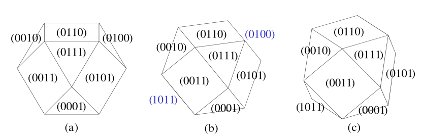
Figure 6: Appearance of the cuboctahedron when one is (a) in the region $-\tilde{\theta}_{1}+\tilde{\theta}_{2}+\tilde{\theta}_{3}>0,~{}\tilde{\theta}_{1}-\tilde{\theta}_{2}+\tilde{\theta}_{3}>0,~{}\tilde{\theta}_{1}+\tilde{\theta}_{2}-\tilde{\theta}_{3}>0$, (b) on the locus $-\tilde{\theta}_{1}+\tilde{\theta}_{2}+\tilde{\theta}_{3}=0,~{}\tilde{\theta}_{2}>0,~{}\tilde{\theta}_{3}>0$, and (c) in the region $-\tilde{\theta}_{1}+\tilde{\theta}_{2}+\tilde{\theta}_{3}<0,~{}\tilde{\theta}_{2}>0,~{}\tilde{\theta}_{3}>0$.

Compared with what occurs geometrically at the same locus, this process should correspond to a flop transition $[C_{1}]\rightarrow-[C_{1}]$, as in section 2. In fact, if we consider the following correspondence between representations and homology classes,

$$(0,1,0,0)\Leftrightarrow[C_{1}],$$

$$(0,0,1,0)\Leftrightarrow[C_{2}],$$ (3.11)

$$(0,0,0,1)\Leftrightarrow[C_{3}],$$

the process exchanging $(0,1,0,0)$ for $(1,0,1,1)$ is interpreted as a flop. The key point is the fact that $(1,1,1,1)$ corresponds to a D0-brane as noted in section 2. Thus the representation $(1,0,1,1)=(1,1,1,1)-(0,1,0,0)$ should correspond to a homology class $[p]-[C_{1}]$ where $[p]$ represents a homology class of a point corresponding to a D0-brane. If we ignore $[p]$ , the exchange $(0,1,0,0)\leftrightarrow(1,0,1,1)$ implies $[C_{1}]\leftrightarrow-[C_{1}]$, which is nothing but the flop transition discussed in section 2. The correspondence (3.11) agrees with the result obtained from the other methods [21, 22].

Here we comment on an implication of the result on the McKay correspondence. The McKay correspondence between representations of $\Gamma$ and geometry of resolutions of ${\bf C}^{3}/\Gamma$ has been mainly discussed for a particular resolution of the orbifold called a Hilbert scheme. In the present case, the Hilbert scheme is the space with a topology represented by the toric diagram in Figure 2(a). The above result can be interpreted as providing a way to calculate the McKay correspondence explicitly for resolutions other than the Hilbert scheme.

3.2 Transitions corresponding to change of coordinates

Next we would like to investigate another type of transition. Start with a point in the region $\tilde{\theta}_{2}>0,~{}\tilde{\theta}_{3}>0$ and $-\tilde{\theta}_{1}+\tilde{\theta}_{2}+\tilde{\theta}_{3}<0$, from which seven surfaces corresponding to (3.10) are visible as shown in Figure 7(a). As the value of $\tilde{\theta}_{2}$ decreases, the area of the surface $(0,1,0,1)$ visible from that point becomes smaller, and it degenerate to a line when one comes to the locus $\tilde{\theta}_{2}=0$. At the same time the surface $(1,0,1,0)$ opposite to $(0,1,0,1)$ becomes visible as a line as in Figure 7(b). As one moves further, the surface $(0,1,0,1)$ completely disappears while the surface $(1,0,1,0)$ appears as in Figure 7(c). Thus $(1,0,1,0)$ replaces $(0,1,0,1)$ as a subrepresentation when one crosses the locus $\tilde{\theta}_{2}=0$.

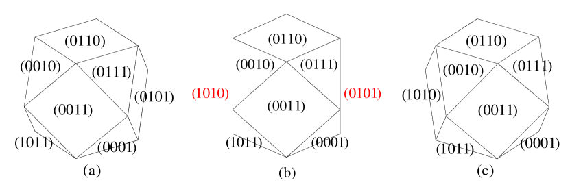
Figure 7: Appearance of the cuboctahedron (a) in the region $\tilde{\theta}_{2}>0,~{}\tilde{\theta}_{3}>0,~{}\tilde{\theta}_{1}-\tilde{\theta}_{2}-\tilde{\theta}_{3}>0$, (b) on the locus $\tilde{\theta}_{2}=0,~{}\tilde{\theta}_{3}>0,~{}\tilde{\theta}_{1}-\tilde{\theta}_{3}>0$, and (c) in the region $\tilde{\theta}_{2}<0,~{}\tilde{\theta}_{3}>0,~{}\tilde{\theta}_{1}+\tilde{\theta}_{2}-\tilde{\theta}_{3}>0$.

Compared with the result in section 2, this process should correspond to a change of homogeneous coordinates from $p_{5}$ to $p_{8}$. For a consistent interpretation of the process, it is found to be necessary to consider the following permutation of subrepresentations,

$$(0,0,1,0)\leftrightarrow(0,1,1,1),\quad(0,0,0,1)\leftrightarrow(1,0,1,1),$$ (3.12)

in addition to the exchange $(0,1,0,1)$ for $(1,0,1,0)$. This transformation of subrepresentations is nothing but the reflection of the cuboctahedron with respect to the plane $\tilde{\theta}_{2}=0$. Similarly, the exchange of the homogeneous coordinates $p_{4}\leftrightarrow p_{7}$ ($p_{6}\leftrightarrow p_{9}$) in the toric method corresponds to the reflection with respect to $\tilde{\theta}_{1}=0$ ($\tilde{\theta}_{3}=0$). We denote the reflection with respect to the plane $\tilde{\theta}_{a}=0$ as $A_{a}$.

To understand the meaning of the exchange of the homogeneous coordinates, we consider the combinations of the reflections; $M_{1}=A_{2}A_{3},~{}M_{2}=A_{3}A_{1},~{}M_{3}=A_{1}A_{2}$. For example, $M_{1}$ corresponds to the action $\tilde{\theta}_{2}\rightarrow-\tilde{\theta}_{2},~{}\tilde{\theta}_{3}\rightarrow-\tilde{\theta}_{3}$, and leads to the following permutation of subrepresentations,

$$(1,0,0,0)\leftrightarrow(0,1,0,0),$$

$$(0,0,1,0)\leftrightarrow(0,0,0,1),$$

$$(0,1,1,1)\leftrightarrow(1,0,1,1),$$

$$(1,1,0,1)\leftrightarrow(1,1,1,0),$$ (3.13)

$$(1,0,1,0)\leftrightarrow(0,1,0,1),$$

$$(1,0,0,1)\leftrightarrow(0,1,1,0).$$

Based on the correspondence between representations and homology classes obtained above, the action $M_{1}$ is geometrically interpreted as

$$[C_{1}]\leftrightarrow[p]-[C_{1}]-[C_{2}]-[C_{3}],\quad[C_{2}]\leftrightarrow[C_{3}].$$ (3.14)

Similarly, the actions $M_{2}$ and $M_{3}$ are represented in terms of geometry. It is known that the actions $M_{i}$ satisfying the relations, $M_{1}^{2}=M_{2}^{2}=M_{3}^{2}=1,\,M_{1}M_{2}=M_{3}$, are interpreted as monodromies around the orbifold point in the K${\rm{\ddot{a}}}$hler moduli space [22].

Thus the change of homogeneous coordinates in the toric method stems from the orbifold monodromy, and the number $c$ of the coordinates in the expression (2.4) can be understood from this viewpoint. As discussed in section 2, the fact that D-branes do not see non-geometric phases comes from the redundancy of the homogeneous coordinates. Thus the above argument shows that this property is a consequence of the monodromy around the orbifold point.

For a few examples other than ${\bf C}^{3}/{\bf Z}_{2}\times{\bf Z}_{2}$, we have verified that the redundancy of homogeneous coordinates in the expression (2.4) can be understood from orbifold monodromy. It would be interesting to have a general expression for the number $c$ of homogeneous coordinates in the expression (2.4) for orbifolds ${\bf C}^{3}/{\bf Z}_{n}$ and ${\bf C}^{3}/{\bf Z}_{n}\times{\bf Z}_{m}$.

3.3 Decay products on marginal stability loci

Finally we would like to discuss decay products at marginal stability loci. They are read off from the cuboctahedron as follows. Subrepresentations on its surfaces visible from a point in the $\tilde{\theta}$-space are interpreted as potential decay products. As one of the surfaces shrinks to a line, decay is triggered by the subrepresentation on this surface since the stability condition (3.2) for this subrepresentation saturates. Remaining elements of the decay must be such that the sum of dimension vectors of decay products is $(1,1,1,1)$. By inspecting the rule of assignment of subrepresentations on the cuboctahedron, one can see that decay products are two subrepresentations on the shrinking surfaces at the marginal stability loci. For example, on the locus $-\tilde{\theta}_{1}+\tilde{\theta}_{2}+\tilde{\theta}_{3}=0$, $(1,1,1,1)$ decays into $(0,1,0,0)$ and $(1,0,1,1)$ as shown in Figure 6(b).

This result agrees with the conjecture on decay products given in [8]. To explain the conjecture, we need to make some definitions. A sequence of subrepresentations of a semi-stable representation $R$,

$$0=R_{0}\subset R_{1}\subset R_{2}\subset...\subset R_{m}=R,$$ (3.15)

is called a Jordan-H${\rm{\ddot{o}}}$lder filtration if the dimension vectors $n_{a}$ of $R_{a}$ satisfy $\theta\cdot n_{a}=0$ and the quotients $M_{a}=R_{a}/R_{a-1}$ are $\theta$-stable. By using a Jordan-H${\rm{\ddot{o}}}$lder filtration, the graded representation of $R$ is defined as

$${\rm gr}(R)=\oplus_{a}M_{a}.$$ (3.16)

Given a semi-stable representation $R$, there may be several Jordan-H${\rm{\ddot{o}}}$lder filtrations but ${\rm gr}(R)$ is unique. We also note that ${\rm gr}(R)$ coincides with $R$ for $\theta$-stable representations. The conjecture given in [8] is that decay products of $R$ on marginal stability loci are given by ${\rm gr}(R)$. In the present case, on the locus $-\tilde{\theta}_{1}+\tilde{\theta}_{2}+\tilde{\theta}_{3}=0$, the representation $R=(1,1,1,1)$ has a Jordan-H${\rm{\ddot{o}}}$lder filtration,

$$(0,0,0,0)\subset(0,1,0,0)\subset(1,1,1,1).$$ (3.17)

It leads ${\rm gr}(R)=(0,1,0,0)\oplus(1,0,1,1)$. Thus D0-brane decays into a threshold bound state of $(0,1,0,0)$ and $(1,0,1,1)$ at $-\tilde{\theta}_{1}+\tilde{\theta}_{2}+\tilde{\theta}_{3}=0$, in agreement with the result read off from the cuboctahedron.

4 Discussions

In this section, we would like to discuss why non-geometric phases are projected out from the viewpoint of stability of D0-branes.

In standard classical geometry, elementary constituents of a space are points; correspondingly, a space probed by a point particle is described by classical geometry. In this paper, we have used a D0-brane as a probe to study the orbifold. Since a D0-brane is a point-like object, it may seem reasonable that a space probed by a D0-brane has a classical geometric interpretation. However, there is an issue we have to care about: stability of a D0-brane. If a D0-brane becomes unstable, it decays into a sum of higher dimensional objects in general, and loses the property as a point-like probe. Thus the most likely expectation is that a space probed by a D0-brane is described by classical geometry only if the D0-brane is stable. This expectation is consistent with the result in this paper. As we have seen, any point in the $\tilde{\theta}$-space where a D0-brane is stable belongs to geometric phases, and the loci on which D0-brane is marginally stable coincide with boundaries of geometric phases. In this respect, the fact that D0-branes are always (semi) stable may be understood as one explanation of the disappearance of non-geometric phases.

Of course, it is not clear that the expectation holds for other cases. It is necessary to examine to what extent the expectation can be applied.

Acknowledgements

We would like to thank Y. Ito, Y. Ohtake and T. Takayanagi for valuable discussions.

References

- [1] M. R. Douglas and G. Moore, “D-branes, quivers, and ALE Instantons,” hep-th/9603167.
- [2] J. McKay, “Graphs, singularities, and finite groups,” Proc. Symp. Pure Math. 37 (1980) 183.
- [3] M. Reid, “McKay correspondence,” alg-geom/9702016.
- [4] Y. Ito and H. Nakajima, “McKay correspondence and Hilbert schemes in dimension three,” math-ag/9803120.
- [5] T. Bridgeland, A. King and M. Reid, “Mukai implies McKay,” math.AG/9908027.
- [6] M. R. Douglas, B. Fiol and C. Romelsberger, “Stability and BPS branes,” hep-th/0002037.
- [7] M. R. Douglas, B. Fiol and C. Romelsberger, “The spectrum of BPS branes on a noncompact Calabi-Yau,” hep-th/0003263.
- [8] B. Fiol and M. Marino, “BPS states and algebras from quivers,” JHEP 0007 (2000) 031 [hep-th/0006189].
- [9] M. R. Douglas, “D-branes, categories and N = 1 supersymmetry,” hep-th/0011017.
- [10] B. Fiol, “The BPS spectrum of N = 2 SU(N) SYM and parton branes,” hep-th/0012079.
- [11] A.D. King, “Moduli of representations of finite dimensional algebras,” Quart. J. Math. Oxford(2) 45 (1994) 515.
- [12] M. R. Douglas, B. R. Greene and D. R. Morrison, “Orbifold resolution by D-branes,” Nucl. Phys. B 506 (1997) 84 [hep-th/9704151].
- [13] T. Muto, “D-branes on orbifolds and topology change,” Nucl. Phys. B 521 (1998) 183 [hep-th/9711090].
- [14] B. R. Greene, “D-brane topology changing transitions,” Nucl. Phys. B 525 (1998) 284 [hep-th/9711124].
- [15] S. Mukhopadhyay and K. Ray, “Conifolds from D-branes,” Phys. Lett. B 423 (1998) 247 [hep-th/9711131].
- [16] C. Beasley, B. R. Greene, C. I. Lazaroiu and M. R. Plesser, “D3-branes on partial resolutions of abelian quotient singularities of Calabi-Yau threefolds,” Nucl. Phys. B 566 (2000) 599 [hep-th/9907186].
- [17] T. Sarkar, “D-brane gauge theories from toric singularities of the form and ,” Nucl. Phys. B 595 (2001) 201 [hep-th/0005166].
- [18] P. S. Aspinwall, B. R. Greene and D. R. Morrison, “Calabi-Yau moduli space, mirror manifolds and spacetime topology change in string theory,” Nucl. Phys. B 416 (1994) 414 [hep-th/9309097].
- [19] E. Witten, “Phases of N = 2 theories in two dimensions,” Nucl. Phys. B 403 (1993) 159 [hep-th/9301042].
- [20] P. S. Aspinwall, B. R. Greene and D. R. Morrison, “Measuring small distances in N=2 sigma models,” Nucl. Phys. B 420 (1994) 184 [hep-th/9311042].
- [21] P. S. Aspinwall and M. R. Plesser, “D-branes, discrete torsion and the McKay correspondence,” JHEP 0102 (2001) 009 [hep-th/0009042].
- [22] X. De la Ossa, B. Florea and H. Skarke, “D-branes on noncompact Calabi-Yau manifolds: K-theory and monodromy,” hep-th/0104254.
- [23] A. Craw, “The McKay correspondence and representations of the McKay quiver,” D. Phil. thesis, University of Warwick (2001).
- [24] P. S. Aspinwall and A. E. Lawrence, “Derived categories and zero-brane stability,” hep-th/0104147.