1 Introduction

Supersymmetry (SUSY) is one of the most promising ideas to solve the hierarchy problem in unified theories [1]. It has been noted for some years that one of the most important issues for SUSY unified theories is to understand the SUSY breaking in our observable world. Many models of SUSY breaking uses some kind of mediation of the SUSY breaking from the hidden sector to our observable sector. Supergravity provides a tree level SUSY breaking effects in our observable sector suppressed by the Planck mass $M_{\rm Pl}$ [2]. Gauge mediation models uses messenger fields to communicate the SUSY breaking at the loop level in our observable sector [3].

Recently there has been an active interest in the “Brane World” scenario where our four-dimensional spacetime is realized on the wall in higher dimensional spacetime [4, 5]. In order to discuss the stability of such a wall, it is often useful to consider SUSY theories as the fundamental theory. Moreover, SUSY theories in higher dimensions are a natural possibility in string theories. These SUSY theories in higher dimensions have $8$ or more supercharges, which should be broken partially if we want to have a phenomenologically viable SUSY unified model in four dimensions. Such a partial breaking of SUSY is nicely obtained by the topological defects [6]. Domain walls or other topological defects preserving part of the original SUSY in the fundamental theory are called the BPS states in SUSY theories. Walls have co-dimension one and typically preserve half of the original SUSY, which are called $1/2$ BPS states [7, 8, 9]. Junctions of walls have co-dimension two and typically preserve a quarter of the original SUSY [10, 11].

Because of the new possibility offered by the brane world scenario, there has been a renewed interest in studies of SUSY breaking. It has been pointed out that the non-BPS topological defects can be a source of SUSY breaking [8] and an explicit realization was considered in the context of families localized in different BPS walls [12]. Models have also been proposed with bulk fields mediating the SUSY breaking from the hidden wall to our wall on which standard model fields are localized [13, 14, 15, 16]. The localization of the various matter wave functions in the extra dimensions was proposed to offer a natural realization of the gaugino-mediation of the SUSY breaking [17]. Recently we have proposed a simple mechanism of SUSY breaking due to the coexistence of different kinds of BPS domain walls and proposed an efficient method to evaluate the SUSY breaking parameters such as the boson-fermion mass-splitting by means of overlap of wave functions involving the Nambu-Goldstone (NG) fermion [18], thanks to the low-energy theorem [19, 20]. We have exemplified these points by taking a toy model in four dimensions, which allows an exact solution of coexisting walls with a three-dimensional effective theory. Although the model is only meta-stable, we were able to show approximate evaluation of the overlap allows us to determine the mass-splitting reliably.

The purpose of this paper is to illustrate our idea of SUSY breaking due to the coexistence of BPS walls by taking a simple soluble model with a stable non-BPS configuration of two walls and to extend our analysis to more realistic case of four-dimensional effective theories. We also examine the consequences of our mechanism in detail.

We propose a SUSY breaking mechanism which requires no messenger fields, nor complicated SUSY breaking sector on any of the walls. We assume that our world is on a wall and SUSY is broken only by the coexistence of another wall with some distance from our wall. We find an ${\cal N}=1$ supersymmetric model in four dimensions which admits an exact solution of a stable non-BPS configuration of two walls and study its properties explicitly. We work out how various soft SUSY breaking terms can arise in our framework. Phenomenological implications are briefly discussed. We also find that effective SUSY breaking scale observed on our wall becomes exponentially small as the distance between two walls grows. The NG fermion is localized on the distant wall and its overlap with the wave functions of physical fields on our wall gives the boson-fermion mass-splitting of physical fields on our wall thanks to a low-energy theorem. We propose that this overlap provides a practical method to evaluate the mass-splitting in models with SUSY breaking due to the coexisting walls.

In the next section, a model is introduced that allows a stable non-BPS two-wall configuration as a classical solution. We have also worked out mode expansion on the two-wall background, three-dimensional effective Lagrangian, and the single-wall approximation for the overlap of mode functions to obtain the mass-splitting. Matter fields are also introduced. Section 3 is devoted to study how various soft breaking terms arise in the three-dimensional effective theory. Soft breaking terms in four-dimensional effective theory are worked out in section 4. Phenomenological implications are discussed in section 5. Additional discussion is given in section 6. Appendix A is devoted to discussing the low-energy theorem in three dimensions and the mixing matrix relating the mass eigenstates and superpartner states. Low-energy theorems in four dimensions are derived in Appendix B. In Appendix C, we derive a relation among the order parameters of the SUSY breaking, the energy density of the configuration and the central charge of the SUSY algebra.

2 SUSY breaking by the coexistence of walls

2.1 Stable non-BPS configuration of two walls

We will describe a simple soluble model for a stable non-BPS configuration that represents two-domain-wall system, in order to illustrate our basic ideas. Here we consider domain walls in four-dimensional spacetime to avoid inessential complications. We introduce a simple four-dimensional Wess-Zumino model as follows.

$$\!\!\!{\cal L} \!\!\!=\bar{\Phi}\Phi|_{\theta^{2}\bar{\theta}^{2}}+W(\Phi)|_{\theta^{2}}+{\rm h.c.},\qquad W(\Phi)=\frac{\Lambda^{3}}{g^{2}}\sin\left(\frac{g}{\Lambda}\Phi\right),$$ (2.1)

where $\Phi$ is a chiral superfield $\Phi(Z^{\mu},\theta)=A(Z^{\mu})+\sqrt{2}\theta\Psi(Z^{\mu})+\theta^{2}F(Z^{\mu})$, $Z^{\mu}\equiv X^{\mu}+i\theta\sigma^{\mu}\bar{\theta}$.
A scale parameter $\Lambda$ has a mass-dimension one and a coupling constant $g$ is dimensionless, and both of them are real positive. In the following, we choose $y=X^{2}$ as the extra dimension and compactify it on $S^{1}$ of radius $R$. Other coordinates are denoted as $x^{m}$ ($m=0,1,3$), i.e., $X^{\mu}=(x^{m},y)$. The bosonic part of the model is

$${\cal L}_{\rm bosonic}=-\partial^{\mu}A^{\ast}\partial_{\mu}A-\frac{\Lambda^{4}}{g^{2}}\left|\cos\left(\frac{g}{\Lambda}A\right)\right|^{2}.$$ (2.2)

The target space of the scalar field $A$ has a topology of a cylinder as shown in Fig.1. This model has two vacua at $A=\pm\pi\Lambda/(2g)$, both lie on the real axis.

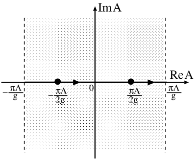
Figure 1: The target space of the scalar field $A$. The line at ${\rm Re}A=\pi\Lambda/g$ and the line at ${\rm Re}A=-\pi\Lambda/g$ are identified each other.

Let us first consider the case of the limit $R\to\infty$. In this case, there are two kinds of BPS domain walls in this model. One of them is

$$A_{\rm cl}^{(1)}(y)=\frac{\Lambda}{g}\left\{2\tan^{-1}e^{\Lambda(y-y_{1})}-\frac{\pi}{2}\right\},$$ (2.3)

which interpolates the vacuum at $A=-\pi\Lambda/(2g)$ to that at $A=\pi\Lambda/(2g)$ as $y$ increases from $y=-\infty$ to $y=\infty$. The other wall is

$$A_{\rm cl}^{(2)}(y)=\frac{\Lambda}{g}\left\{-2\tan^{-1}e^{-\Lambda(y-y_{2})}+\frac{3\pi}{2}\right\},$$ (2.4)

which interpolates the vacuum at $A=\pi\Lambda/(2g)$ to that at $A=3\pi\Lambda/(2g)=-\pi\Lambda/(2g)$. Here $y_{1}$ and $y_{2}$ are integration constants and represent the location of the walls along the extra dimension. The four-dimensional supercharge $Q_{\alpha}$ can be decomposed into two two-component Majorana supercharges $Q^{(1)}_{\alpha}$ and $Q^{(2)}_{\alpha}$ which can be regarded as supercharges in three dimensions

$$Q_{\alpha}=\frac{1}{\sqrt{2}}(Q^{(1)}_{\alpha}+iQ^{(2)}_{\alpha}).$$ (2.5)

Each wall breaks a half of the bulk supersymmetry: $Q^{(1)}_{\alpha}$ is broken by $A_{\rm cl}^{(2)}(y)$, and $Q^{(2)}_{\alpha}$ by $A_{\rm cl}^{(1)}(y)$. Thus all of the bulk supersymmetry will be broken if these walls coexist.

We will consider such a two-wall system to study the SUSY breaking effects in the low-energy three-dimensional theory on the background. The field configuration of the two walls will wrap around the cylinder in the target space of $A$ as $y$ increases from $0$ to $2\pi R$. Such a configuration should be a solution of the equation of motion,

$$\partial^{\mu}\partial_{\mu}A+\frac{\Lambda^{3}}{g}\sin\left(\frac{g}{\Lambda}A^{\ast}\right)\cos\left(\frac{g}{\Lambda}A\right)=0.$$ (2.6)

We can easily show that the minimum energy static configuration with unit winding number should be real. We find that a general real static solution of Eq.(2.6) that depends only on $y$ is

$$A_{\rm cl}(y)=\frac{\Lambda}{g}{\rm am}\left(\frac{\Lambda}{k}(y-y_{0}),k\right),$$ (2.7)

where $k$ and $y_{0}$ are real parameters and the function ${\rm am}(u,k)$ denotes the amplitude function, which is defined as an inverse function of

$$u(\varphi)=\int_{0}^{\varphi}\frac{{\rm d}\theta}{\sqrt{1-k^{2}\sin^{2}\theta}}.$$ (2.8)

If $k>1$, it becomes a periodic function with the period $4K(1/k)/\Lambda$, where the function $K(k)$ is the complete elliptic integral of the first kind. If $k<1$, the solution $A_{\rm cl}(y)$ is a monotonically increasing function with

$$A_{\rm cl}\left(y+{4kK(k)\over\Lambda}\right)=A_{\rm cl}(y)+2\pi{\Lambda\over g}.$$ (2.9)

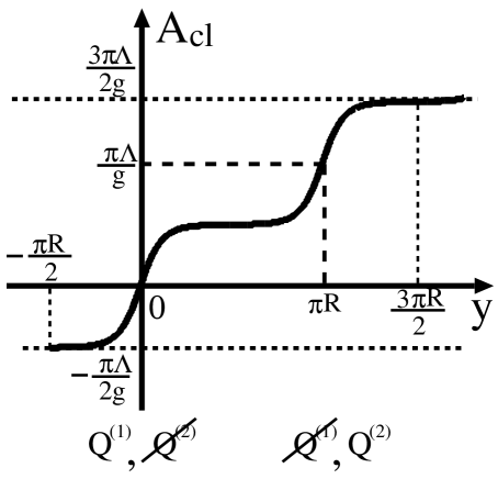
Figure 2: The profile of the classical solution $A_{\rm cl}(y)$. The dotted lines $A=-\pi\Lambda/(2g)$ and $A=3\pi\Lambda/(2g)$ are identified.

This is the solution that we want. Since the field $A$ is an angular variable $A=A+2\pi\Lambda/g$, we can choose the compactified radius $2\pi R=4kK(k)/\Lambda$ so that the classical field configuration $A_{\rm cl}(y)$ contains two walls and becomes periodic modulo $2\pi\Lambda/g$. We shall take $y_{0}=0$ to locate one of the walls at $y=0$. Then we find that the other wall is located at the anti-podal point $y=\pi R$ of the compactified circle. We have computed the energy of a superposition of the first wall $A_{\rm cl}^{(1)}(y)$ located at $y=y_{1}$in Eq.(2.3) and the second wall $A_{\rm cl}^{(2)}(y)$ located at $y=y_{2}$ in Eq.(2.4). This energy can be regarded as a potential between two walls in the adiabatic approximation and has a peak at $|y_{1}-y_{2}|=0$ implying that two walls experience a repulsion. This is in contrast to a BPS configuration of two walls which should exert no force between them. Thus we can explain that the second wall is settled at the anti-podal point $y=\pi R$ in our stable non-BPS configuration because of the repulsive force between two walls.

In the limit of $R\to\infty$, i.e., $k\to 1$, $A_{\rm cl}(y)$ approaches to the BPS configuration $A_{\rm cl}^{(1)}(y)$ with $y_{1}=0$ near $y=0$, which preserves $Q^{(1)}$, and to $A_{\rm cl}^{(2)}(y)$ with $y_{2}=\pi R$ near $y=\pi R$, which preserves $Q^{(2)}$. The profile of the classical solution $A_{\rm cl}(y)$ is shown in Fig.2. We will refer to the wall at $y=0$ as “our wall” and the wall at $y=\pi R$ as “the other wall”.

2.2 The fluctuation mode expansion

Let us consider the fluctuation fields around the background $A_{\rm cl}(y)$,

$$A(X) \!\!= \!\!A_{\rm cl}(y)+\frac{1}{\sqrt{2}}(A_{\rm R}(X)+iA_{\rm I}(X)),$$

$$\Psi_{\alpha}(X) \!\!= \!\!\frac{1}{\sqrt{2}}(\Psi_{\alpha}^{(1)}(X)+i\Psi_{\alpha}^{(2)}(X)).$$ (2.10)

To expand them in modes, we define the mode functions as solutions of equations:

$$\left\{-\partial_{y}^{2}-\Lambda^{2}\cos\left(\frac{2g}{\Lambda}A_{\rm cl}(y)\right)\right\}b_{{\rm R},p}(y) \!\!= \!\!m_{{\rm R},p}^{2}b_{{\rm R},p}(y),$$

$$\{-\partial_{y}^{2}+\Lambda^{2}\}b_{{\rm I},p}(y) \!\!= \!\!m_{{\rm I},p}^{2}(y)b_{{\rm I},p}(y),$$ (2.11)

$$\left\{-\partial_{y}-\Lambda\sin\left(\frac{g}{\Lambda}A_{\rm cl}(y)\right)\right\}f^{(1)}_{p}(y) \!\!= \!\!m_{p}f^{(2)}_{p}(y),$$

$$\left\{\partial_{y}-\Lambda\sin\left(\frac{g}{\Lambda}A_{\rm cl}(y)\right)\right\}f^{(2)}_{p}(y) \!\!= \!\!m_{p}f^{(1)}_{p}(y).$$ (2.12)

The four-dimensional fluctuation fields can be expanded as

$$A_{\rm R}(X)=\sum_{p}b_{{\rm R},p}(y)a_{{\rm R},p}(x),\;\;\;A_{\rm I}(X)=\sum_{p}b_{{\rm I},p}(y)a_{{\rm I},p}(x),$$ (2.13)

$$\Psi^{(1)}(X)=\sum_{p}f^{(1)}_{p}(y)\psi^{(1)}_{p}(x),\;\;\;\Psi^{(2)}(X)=\sum_{p}f^{(2)}_{p}(y)\psi^{(2)}_{p}(x).$$ (2.14)

As a consequence of the linearized equation of motion, the coefficient $a_{{\rm R},p}(x)$ and $a_{{\rm I},p}(x)$ are scalar fields in three-dimensional effective theory with masses $m_{{\rm R},p}$ and $m_{{\rm I},p}$, and $\psi^{(1)}_{p}(x)$ and $\psi^{(2)}_{p}(x)$ are three-dimensional spinor fields with masses $m_{p}$, respectively.

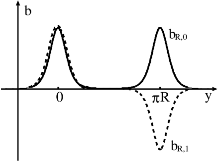
Figure 3: The mode functions for the bosonic modes $a_{{\rm R},0}$ and $a_{{\rm R},1}$. The solid line represents the profile of $b_{{\rm R},0}(y)$ and the dashed line is that of $b_{{\rm R},1}(y)$.

Exact mode functions and mass-eigenvalues are known for several light modes of $b_{{\rm R},p}(y)$,

$$b_{{\rm R},0}(y) \!\!= \!\!C_{{\rm R},0}{\rm dn}\left(\frac{\Lambda y}{k},k\right),\;\;\;m_{{\rm R},0}^{2}=0,$$

$$b_{{\rm R},1}(y) \!\!= \!\!C_{{\rm R},1}{\rm cn}\left(\frac{\Lambda y}{k},k\right),\;\;\;m_{{\rm R},1}^{2}=\frac{1-k^{2}}{k^{2}}\Lambda^{2},$$

$$b_{{\rm R},2}(y) \!\!= \!\!C_{{\rm R},2}{\rm sn}\left(\frac{\Lambda y}{k},k\right),\;\;\;m_{{\rm R},2}^{2}=\frac{\Lambda^{2}}{k^{2}},$$ (2.15)

where functions ${\rm dn}(u,k)$, ${\rm cn}(u,k)$, ${\rm sn}(u,k)$ are the Jacobi’s elliptic functions and $C_{{\rm R},p}$ are normalization factors. For $b_{{\rm I},p}(y)$, we can find all the eigenmodes

$$b_{{\rm I},p}(y)=\frac{1}{\sqrt{2\pi R}}{\rm e}^{i{p\over R}y},\;\;\;m_{{\rm I},p}^{2}=\Lambda^{2}+\frac{p^{2}}{R^{2}},\;\;\;(p\in{\bf Z}).$$ (2.16)

The massless field $a_{{\rm R},0}(x)$ is the Nambu-Goldstone (NG) boson for the breaking of the translational invariance in the extra dimension. The first massive field $a_{{\rm R},1}(x)$ corresponds to the oscillation of the background wall around the anti-podal equilibrium point and hence becomes massless in the limit of $R\rightarrow\infty$. All the other bosonic fields remain massive in that limit.

For fermions, only zero modes are known explicitly,

$$f^{(1)}_{0}(y)=C_{0}\left\{{\rm dn}\left(\frac{\Lambda y}{k},k\right)+k{\rm cn}\left(\frac{\Lambda y}{k},k\right)\right\},\;\;\;f^{(2)}_{0}(y)=C_{0}\left\{{\rm dn}\left(\frac{\Lambda y}{k},k\right)-k{\rm cn}\left(\frac{\Lambda y}{k},k\right)\right\},$$ (2.17)

where $C_{0}$ is a normalization factor. These fermionic zero modes are the NG fermions for the breaking of $Q^{(1)}$-SUSY and $Q^{(2)}$-SUSY, respectively.

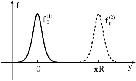
Figure 4: The mode functions for fermionic zero-modes $\psi^{(1)}_{0}$ and $\psi^{(2)}_{0}$. The solid line represents the profile of $f^{(1)}_{0}(y)$ and the dashed line is that of $f^{(2)}_{0}(y)$.

Thus there are four fields which are massless or become massless in the limit of $R\rightarrow\infty$: $a_{{\rm R},0}(x)$, $a_{{\rm R},1}(x)$, $\psi^{(1)}_{0}(x)$ and $\psi^{(2)}_{0}(x)$. The profiles of their mode functions are shown in Fig.3 and Fig.4. Other fields are heavier and have masses of the order of $\Lambda$.

In the following discussion, we will concentrate ourselves on the breaking of the $Q^{(1)}$-SUSY, which is approximately preserved by our wall at $y=0$. So we call the field $\psi^{(2)}_{0}(x)$ the NG fermion in the rest of the paper.

2.3 Three-dimensional effective Lagrangian

We can obtain a three-dimensional effective Lagrangian by substituting the mode-expanded fields Eq.(2.13) and Eq.(2.14) into the Lagrangian (2.1), and carrying out an integration over $y$

$${\cal L}^{(3)} \!\!\!= \!\!\!-V_{0}-\frac{1}{2}\partial^{m}a_{{\rm R},0}\partial_{m}a_{{\rm R},0}-\frac{1}{2}\partial^{m}a_{{\rm R},1}\partial_{m}a_{{\rm R},1}-\frac{i}{2}\psi^{(1)}_{0}\partial/\psi^{(1)}_{0}-\frac{i}{2}\psi^{(2)}_{0}\partial/\psi^{(2)}_{0}$$ (2.18)

$$\!\!\!-\frac{1}{2}m_{{\rm R},1}^{2}a_{{\rm R},1}^{2}+g_{{\rm eff}}a_{{\rm R},1}\psi^{(1)}_{0}\psi^{(2)}_{0}+\cdots,$$

where $\partial/\equiv\gamma^{m}_{(3)}\partial_{m}$ and an abbreviation denotes terms involving heavier fields and higher-dimensional terms. Here $\gamma$-matrices in three dimensions are defined by $\left(\gamma^{m}_{(3)}\right)\equiv\left(-\sigma^{2},i\sigma^{3},-i\sigma^{1}\right)$. The vacuum energy $V_{0}$ is given by the energy density of the background and thus

$$V_{0}\equiv\int^{\pi R}_{-\pi R}{\rm d}y\left\{\left(\partial_{y}A_{\rm cl}\right)+\frac{\Lambda^{4}}{g^{2}}\cos^{2}\left(\frac{g}{\Lambda}A_{\rm cl}\right)\right\}=\frac{\Lambda^{3}}{g^{2}k}\int_{-2K(k)}^{2K(k)}{\rm d}u\left\{(1+k^{2})-2k^{2}{\rm sn}^{2}(u,k)\right\},$$ (2.19)

and the effective Yukawa coupling $g_{{\rm eff}}$ is

$$g_{{\rm eff}}\equiv\frac{g}{\sqrt{2}}\int^{\pi R}_{-\pi R}{\rm d}y\,\cos\left(\frac{g}{\Lambda}A_{\rm cl}(y)\right)b_{{\rm R},1}(y)f^{(1)}_{0}(y)f^{(2)}_{0}(y)=\frac{g}{\sqrt{2}}\frac{C_{0}^{2}}{C_{{\rm R},1}}(1-k^{2}).$$ (2.20)

In the limit of $R\to\infty$, the parameters $m_{{\rm R},1}$ and $g_{{\rm eff}}$ vanish and thus we can redefine the bosonic massless fields as

$$\left(\begin{array}[]{c}a^{(1)}_{0}\\ a^{(2)}_{0}\end{array}\right)=\frac{1}{\sqrt{2}}\left(\begin{array}[]{cc}1&1\\ -1&1\end{array}\right)\left(\begin{array}[]{c}a_{{\rm R},0}\\ a_{{\rm R},1}\end{array}\right).$$ (2.21)

In this case, the fields $a^{(1)}_{0}(x)$ and $\psi^{(1)}_{0}(x)$ form a supermultiplet for $Q^{(1)}$-SUSY and their mode functions are both localized on our wall. The fields $a^{(2)}_{0}(x)$ and $\psi^{(2)}_{0}(x)$ are singlets for $Q^{(1)}$-SUSY and are localized on the other wall.

When the distance between the walls $\pi R$ is finite, $Q^{(1)}$-SUSY is broken and the mass-splittings between bosonic and fermionic modes are induced. The mass squared $m_{{\rm R},1}^{2}$ in Eq.(2.18) corresponds to the difference of the mass squared $\Delta m^{2}$ between $a^{(1)}_{0}(x)$ and $\psi^{(1)}_{0}(x)$ since the fermionic mode $\psi^{(1)}_{0}(x)$ is massless. Besides the mass terms, we can read off the SUSY breaking effects from the Yukawa couplings like $g_{{\rm eff}}$.

We have noticed in Ref.[18] that these two SUSY breaking parameters, $m_{{\rm R},1}$ and $g_{{\rm eff}}$, are related by the low-energy theorem associated with the spontaneous breaking of SUSY. In our case, the low-energy theorem becomes

$$\frac{g_{{\rm eff}}}{m_{{\rm R},1}^{2}}=\frac{1}{2f}.$$ (2.22)

where $f$ is an order parameter of the SUSY breaking, and it is given by the square root of the vacuum (classical background) energy density $V_{0}$ in Eq.(2.19). The low-energy theorem in three dimensions is briefly explained in Appendix A.1. Since the superpartner of the fermionic field $\psi^{(1)}_{0}(x)$ is a mixture of mass-eigenstates, we had to take into account the mixing Eq.(2.21). The mixing in general situation is discussed and is applied to the present case in Appendix A.2 and A.3.

Figure 5: The logarithm of the mass-splitting as a function of the distance between the wall. The horizontal axis is the wall distance normalized by $1/\Lambda$.

Fig.5 shows the mass-splitting $\Delta m^{2}$ as a function of the wall distance $\pi R$. As this figure shows, the mass-splitting decays exponentially as the wall distance increases. This is one of the characteristic features of our SUSY breaking mechanism. This fact can be easily understood by remembering the profile of each modes. Note that the mass-splitting $\Delta m^{2}(=m_{{\rm R},1}^{2})$ is proportional to the effective Yukawa coupling constant $g_{{\rm eff}}$, which is represented by an overlap integral of the mode functions. Here the mode functions of the fermionic field $\psi^{(1)}_{0}(x)$ and its superpartner are both localized on our wall, and that of the NG fermion $\psi^{(2)}_{0}(x)$ is localized on the other wall. Therefore the mass-splitting becomes exponentially small when the distance between the walls increases, because of exponentially dumping tails of the mode functions.

2.4 Single-wall approximation

Next we will propose a practical method of estimation for the mass-splittings. We often encounter the case where single-BPS-domain-wall solutions are known but exact two-wall configurations are not. This is because the latter are solutions of a second order differential equation, namely the equation of motion, while the former are solutions of first order differential equations, namely BPS equations. We can estimate the mass-splitting by using only informations on the single-wall background, even if two-wall configurations are not known. As mentioned in the previous subsection, the mass-splitting $\Delta m^{2}$ is related to the coupling constant $g_{{\rm eff}}$ and the order parameter $f$. So we can estimate $\Delta m^{2}$ by calculating $g_{{\rm eff}}$ and $f$.

When two walls are far apart, the energy of the background $V_{0}$ in Eq.(2.19) can be well-approximated by the sum of those of our wall and of the other wall.

$$V_{0}\simeq 2\frac{\Lambda^{3}}{g^{2}}\int_{-\infty}^{\infty}{\rm d}u\left\{2-2\tanh^{2}u\right\}=\frac{8\Lambda^{3}}{g^{2}}.$$ (2.23)

Considering the profiles of background and mode functions, we can see that the main contributions to the overlap integral of $g_{{\rm eff}}$ come from neighborhood of our wall and the other wall. These two regions give the same numerical contributions to the integral, including their signs. Thus we can obtain $g_{{\rm eff}}$ by calculating the overlap integral of approximate background and mode functions which well approximate their behaviors near our wall, and multiplying it by two.

In the neighborhood of our wall, the two-wall background $A_{\rm cl}(y)$ can be well approximated by the single-wall background $A_{\rm cl}^{(1)}(y)$ with $y_{1}=0$. So,

$$\cos\left(\frac{g}{\Lambda}A_{\rm cl}(y)\right)\simeq\cos\left(\frac{g}{\Lambda}A_{\rm cl}^{(1)}(y)\right)=\frac{1}{\cosh(\Lambda y)}.$$ (2.24)

Next, we will proceed to the approximation of mode functions. From the mode equations in Eq.(2.12), we can express the zero-modes $f^{(1)}_{0}(y)$ and $f^{(2)}_{0}(y)$ as

$$f^{(1)}_{0}(y) \!\!= \!\!C_{{\rm f},0}^{(1)}e^{-\int_{0}^{y}{\rm d}y^{\prime}\Lambda\sin\left(\frac{g}{\Lambda}A_{\rm cl}(y^{\prime})\right)},$$ (2.25)

$$f^{(2)}_{0}(y) \!\!= \!\!C_{{\rm f},0}^{(2)}e^{\int_{0}^{y}{\rm d}y^{\prime}\Lambda\sin\left(\frac{g}{\Lambda}A_{\rm cl}(y^{\prime})\right)},$$ (2.26)

where $C_{{\rm f},0}^{(1)}$ and $C_{{\rm f},0}^{(2)}$ are normalization factors.

Since the function $f^{(1)}_{0}(y)$ has its support mainly on our wall, it is simply approximated near our wall by

$$f^{(1)}_{0}(y)\simeq C_{{\rm f},0}^{(1)}e^{-\int_{0}^{y}{\rm d}y^{\prime}\Lambda\sin\left(\frac{g}{\Lambda}A_{\rm cl}^{(1)}(y^{\prime})\right)}=\frac{C_{{\rm f},0}^{(1)}}{\cosh(\Lambda y)}.$$ (2.27)

Then we can determine $C_{{\rm f},0}^{(1)}=\sqrt{\Lambda/2}$ by the normalization condition.

Similarly, the mode $f^{(2)}_{0}(y)$ can be approximated near our wall by

$$f^{(2)}_{0}(y)\simeq C_{{\rm f},0}^{(2)}e^{\int_{0}^{y}{\rm d}y^{\prime}\Lambda\sin\left(\frac{g}{\Lambda}A_{\rm cl}^{(1)}(y^{\prime})\right)}=C_{{\rm f},0}^{(2)}\cosh(\Lambda y).$$ (2.28)

Unlike the case of $f^{(1)}_{0}(y)$, however, we cannot determine $C_{{\rm f},0}^{(2)}$ by using this approximate expression because the mode $f^{(2)}_{0}(y)$ is localized mainly on the other wall. Here it should be noted that $f^{(2)}_{0}(y)=f^{(1)}_{0}(y-\pi R)$ from Eq.(2.12) and the property of the background: $A_{\rm cl}(y-\pi R)=A_{\rm cl}(y)-\pi\Lambda/g$. Thus,

$$f^{(2)}_{0}(y) \!\!= \!\!C_{{\rm f},0}^{(1)}e^{-\int_{0}^{y-\pi R}{\rm d}y^{\prime}\Lambda\sin\left(\frac{g}{\Lambda}A_{\rm cl}(y^{\prime})\right)}=C_{{\rm f},0}^{(1)}e^{\int_{\pi R}^{y}{\rm d}y^{\prime}\Lambda\sin\left(\frac{g}{\Lambda}A_{\rm cl}(y^{\prime})\right)}$$ (2.29)

$$\!\!= \!\!C_{{\rm f},0}^{(1)}e^{-\int_{0}^{\pi R}{\rm d}y^{\prime}\Lambda\sin\left(\frac{g}{\Lambda}A_{\rm cl}(y^{\prime})\right)}e^{\int_{0}^{y}{\rm d}y^{\prime}\Lambda\sin\left(\frac{g}{\Lambda}A_{\rm cl}(y^{\prime})\right)},$$

and we can obtain a relation:

$$C_{{\rm f},0}^{(2)}=C_{{\rm f},0}^{(1)}e^{-\int_{0}^{\pi R}{\rm d}y^{\prime}\Lambda\sin\left(\frac{g}{\Lambda}A_{\rm cl}(y^{\prime})\right)}.$$ (2.30)

In the region of $y\in[0,\pi R]$, the background is well approximated by

$$A_{\rm cl}(y)\simeq\left\{\begin{array}[]{l}A_{\rm cl}^{(1)}(y)\;\;\;(0\leq y<\frac{\pi R}{2})\\ A_{\rm cl}^{(2)}(y)\;\;\;(\frac{\pi R}{2}<y\leq\pi R)\end{array}\right.$$ (2.31)

with $y_{1}=0$ and $y_{2}=\pi R$, and thus

$$\sin\left(\frac{g}{\Lambda}A_{\rm cl}(y)\right) \!\!\simeq \!\!\left\{\begin{array}[]{l}\sin\left(\frac{g}{\Lambda}A_{\rm cl}^{(1)}(y)\right)=\tanh(\Lambda y)\;\;\;(0\leq y<\frac{\pi R}{2})\\ \sin\left(\frac{g}{\Lambda}A_{\rm cl}^{(2)}(y)\right)=-\tanh(\Lambda(y-\pi R))\;\;\;(\frac{\pi R}{2}<y\leq\pi R)\end{array}\right.$$ (2.34)

$$\!\!\simeq \!\!\tanh(\Lambda y)-\tanh(\Lambda(y-\pi R))-1.$$ (2.35)

Thus the normalization factor can be estimated as

$$C_{{\rm f},0}^{(2)}=C_{{\rm f},0}^{(1)}\frac{e^{\Lambda\pi R}}{\cosh^{2}\Lambda\pi R}\simeq 2\sqrt{2\Lambda}e^{-\Lambda\pi R}.$$ (2.36)

Here we used the fact that $C_{{\rm f},0}^{(1)}=\sqrt{\Lambda/2}$ and $\Lambda\pi R\gg 1$. As a result, the mode function of the NG fermion $f^{(2)}_{0}(y)$ can be approximated near our wall by

$$f^{(2)}_{0}(y)=2\sqrt{2\Lambda}e^{-\Lambda\pi R}\cosh(\Lambda y).$$ (2.37)

In the limit of $R\to\infty$, the $Q^{(1)}$-SUSY is recovered and thus the mode function of the bosonic field $a^{(1)}_{0}(x)$ in Eq.(2.21), $b^{(1)}_{0}(y)$, is identical to $f^{(1)}_{2}(y)$. However, when the other wall exist at finite distance from our wall, this bosonic field is mixed with the field $a^{(2)}_{0}(x)$ localized on the other wall. Because the masses of these two fields $a^{(1)}_{0}(x)$ and $a^{(2)}_{0}(x)$ are degenerate (both are massless), the maximal mixing occurs. (See Eq.(2.21).)

$$\left(\begin{array}[]{c}b_{{\rm R},0}\\ b_{{\rm R},1}\end{array}\right)=\frac{1}{\sqrt{2}}\left(\begin{array}[]{cc}1&-1\\ 1&1\end{array}\right)\left(\begin{array}[]{c}b^{(1)}_{0}\\ b^{(2)}_{0}\end{array}\right),$$ (2.38)

where $b^{(2)}_{0}(y)$ is the mode function of $a^{(2)}_{0}(y)$. Thus the mode function of the mass-eigenmode $b_{{\rm R},1}(y)$ is approximated near our wall by

$$b_{{\rm R},1}(y)\simeq\frac{1}{\sqrt{2}}f^{(1)}_{0}(y)\simeq\frac{\sqrt{\Lambda}}{2}\frac{1}{\cosh(\Lambda y)}.$$ (2.39)

Then by using Eqs.(2.24), (2.27), (2.37) and (2.39), we can obtain the effective Yukawa coupling constant $g_{{\rm eff}}$,

$$g_{{\rm eff}}\simeq 2g\sqrt{2\Lambda}e^{-\Lambda\pi R}.$$ (2.40)

As a result, the approximate mass-splitting value $m_{{\rm R},1}^{({\rm ap})2}$ is estimated as

$$m_{{\rm R},1}^{({\rm ap})2}=2fg_{{\rm eff}}=16\Lambda^{2}e^{-\Lambda\pi R},$$ (2.41)

by using Eq.(2.23) and the low-energy theorem Eq.(2.22). From this expression, we can explicitly see its exponential dependence of the distance between the walls. We call this method of estimation the single-wall approximation.

Figure 6: The ratio of the approximate value $m_{{\rm R},1}^{({\rm ap})2}$ to the exact one $m_{{\rm R},1}^{2}$ as a function of the wall distance $\pi R$. The horizontal axis is normalized by $1/\Lambda$.

In our model, we know the exact mass-eigenvalue $m_{{\rm R},1}^{2}$. So we can check the validity of the above approximation by comparing the approximate value $m_{{\rm R},1}^{({\rm ap})2}$ and the exact one $m_{{\rm R},1}^{2}$. Fig.6 shows the ratio of $m_{{\rm R},1}^{({\rm ap})2}$ to $m_{{\rm R},1}^{2}$ as a function of the wall distance $\pi R$. As this figure shows, we can conclude that the single-wall approximation is very well.

2.5 Matter fields

Let us introduce a matter chiral superfield

$$\Phi_{\rm m}=A_{\rm m}+\sqrt{2}\theta\Psi_{\rm m}+\theta^{2}F_{\rm m},$$ (2.42)

interacting with $\Phi$ in the original Lagrangian (2.1) through an additional superpotential

$$W_{\rm int}=-h\frac{\Lambda}{g}\sin\left(\frac{g}{\Lambda}\Phi\right)\Phi_{\rm m}^{2}=-h\Phi\Phi_{\rm m}^{2}+\cdots,$$ (2.43)

which will be treated as a small perturbation.

Let us decompose the matter fermion $\Psi_{\rm m}(X)$ into two real two-component spinors $\Psi_{{\rm m}\alpha}^{(1)}(X)$ and $\Psi_{{\rm m}\alpha}^{(2)}(X)$ as $\Psi_{{\rm m}\alpha}=(\Psi_{{\rm m}\alpha}^{(1)}+i\Psi_{{\rm m}\alpha}^{(2)})/\sqrt{2}$. Then these fluctuation fields can be expanded by the mode functions as follows.

$$\Psi_{\rm m}^{(1)}(X)=\sum_{p}f^{(1)}_{{\rm m}p}(y)\psi^{(1)}_{{\rm m}p}(x),\;\;\;\Psi_{\rm m}^{(2)}(X)=\sum_{p}f^{(2)}_{{\rm m}p}(y)\psi^{(2)}_{{\rm m}p}(x).$$ (2.44)

The mode equations are defined as

$$\left\{-\partial_{y}-\frac{2h}{g}\Lambda\sin\left(\frac{g}{\Lambda}A_{\rm cl}\right)\right\}f^{(1)}_{{\rm m}p}(y) \!\!= \!\!m_{{\rm m}p}f^{(2)}_{{\rm m}p}(y),$$

$$\left\{\partial_{y}-\frac{2h}{g}\Lambda\sin\left(\frac{g}{\Lambda}A_{\rm cl}\right)\right\}f^{(2)}_{{\rm m}p}(y) \!\!= \!\!m_{{\rm m}p}f^{(1)}_{{\rm m}p}(y).$$ (2.45)

Thus zero-modes on the two-wall background (2.7) can be solved exactly

$$f^{(1)}_{{\rm m}0}(y) \!\!= \!\!C_{{\rm m}0}\left\{{\rm dn}\left(\frac{\Lambda y}{k},k\right)+k{\rm cn}\left(\frac{\Lambda y}{k},k\right)\right\}^{\frac{2h}{g}},$$

$$f^{(2)}_{{\rm m}0}(y) \!\!= \!\!C_{{\rm m}0}\left\{{\rm dn}\left(\frac{\Lambda y}{k},k\right)-k{\rm cn}\left(\frac{\Lambda y}{k},k\right)\right\}^{\frac{2h}{g}}.$$ (2.46)

the mode $f^{(1)}_{{\rm m}0}(y)$ is localized on our wall and the mode $f^{(2)}_{{\rm m}0}(y)$ is on the other wall.

Besides these zero-modes, there are several light modes of $\Phi_{\rm m}$ localized on our wall when the coupling $h$ is taken to be larger than $g$. Those non-zero-modes can be obtained analytically in the limit of $R\to\infty$. For example, the low-lying mass-eigenvalues are discrete at $m_{{\rm m}p}^{2}=p(-p+4h/g)\Lambda^{2}$ with $p=0,1,2,\cdots<2h/g$, and the corresponding mode functions $f^{(1)}_{{\rm m}p}(y)$ for the fields $\psi^{(1)}_{{\rm m}p}(x)$ are

$$f^{(1)}_{{\rm m}p}(y)=\frac{C_{{\rm m}p}}{[\cosh(\Lambda y)]^{\frac{2h}{g}-p}}F\left(-p,1-p+\frac{4h}{g},1-p+\frac{2h}{g};\frac{1-\tanh(\Lambda y)}{2}\right),$$ (2.47)

where $F(\alpha,\beta,\gamma;z)$ is the hypergeometric function and $C_{{\rm m}p}$ is normalization factors. The mode functions $f^{(2)}_{{\rm m}p}(y)$ for the fields $\psi^{(2)}_{{\rm m}p}(x)$ have forms similar to those of $f^{(1)}_{{\rm m}p}(y)$.

Although we do not know the exact mass-eigenvalues and mode functions in the case that the wall distance is finite, we can estimate the boson-fermion mass-splittings $\Delta m^{2}_{p}$ by using the single-wall approximation discussed in the previous subsection. For example, let us estimate the mass-splitting between $\psi^{(1)}_{{\rm m}p}(x)$ and its superpartner $a_{{\rm m}p}^{(1)}(x)$. After including an interaction like Eq.(2.43), the effective Lagrangian has the following Yukawa coupling terms.

$${\cal L}_{\rm int}^{(3)}=\sum_{p}h_{{\rm eff}p}a_{{\rm m}p}^{(1)}\psi^{(1)}_{{\rm m}p}\psi^{(2)}_{0}+{\rm h.c.}+\cdots,$$ (2.48)

$$h_{{\rm eff}p}=\sqrt{2}h\int_{-\pi R}^{\pi R}{\rm d}y\cos\left(\frac{g}{\Lambda}A_{\rm cl}(y)\right)b_{{\rm m}p}^{(1)}(y)f^{(1)}_{{\rm m}p}(y)f^{(2)}_{0}(y).$$ (2.49)

Just like the case of $a^{(1)}_{0}(x)$ and $a^{(2)}_{0}(x)$, the degenerate states $a_{{\rm m}p}^{(1)}(x)$ and $a_{{\rm m}p}^{(2)}(x)$ are maximally mixed with each other and their masseigenvalues split into two different values $m_{{\rm mR}2p}$ and $m_{{\rm mR}(2p+1)}$. By calculating the effective coupling $h_{{\rm eff}p}$ in Eq.(2.49) in the single-wall approximation, we can obtain the following mass-splitting. (See Appendix A.3.4.)

$$\Delta m^{2}_{p}\equiv\frac{m_{{\rm mR}2p}^{2}+m_{{\rm mR}(2p+1)}^{2}}{2}-m_{{\rm m}p}^{2}.$$ (2.50)

Thanks to the approximate supersymmetry, $Q^{(1)}$-SUSY, we can use the mode function in Eq.(2.47) as both $f^{(1)}_{{\rm m}p}(y)$ and $b_{{\rm m}p}^{(1)}(y)$. Then we obtain the mass-splitting in the single wall approximation

$$\Delta m^{2}_{p}=\sqrt{2}fh_{{\rm eff}p}=\frac{16h}{g}\Lambda^{2}e^{-\Lambda\pi R}.$$ (2.51)

This result is independent of the level number $p$. However, it is not a general feature of our SUSY breaking mechanism. It depends on the choice of the interaction $W_{\rm int}$. If we choose $W_{\rm int}=-h\Phi\Phi_{\rm m}^{2}$ as an example, we will obtain a different result that $\Delta m^{2}_{p}$ becomes larger as $p$ increases, just like the result in Ref.[18].

3 Soft SUSY breaking terms in 3D effective theory

In this section, we discuss how various soft SUSY breaking terms in the three-dimensional effective theory are induced in our framework.

Firstly, we discuss a multi-linear scalar coupling, a generalization of the so-called A-term. Such a “generalized A-term” is generated from the following superpotential term in the bulk theory

$$S_{\mbox{\scriptsize A-term}} \!\!\!= \!\!\!\int\!\!{\rm d}^{4}X\left.\frac{{\cal F}\left(\Phi(X,\theta)/M\right)}{M^{N-3}}\Phi_{i_{1}}(X,\theta)\cdots\Phi_{i_{N}}(X,\theta)\right|_{\theta^{2}}+{\rm h.c.}$$ (3.1)

$$\!\!\!\supset \!\!\!\int\!\!{\rm d}^{4}X\frac{{\cal F}^{\prime}(A_{\rm cl}(y)/M)F_{\rm cl}(y)}{M^{N-2}}A_{i_{1}}(X)\cdots A_{i_{N}}(X)+{\rm h.c.},$$

$$\!\!\!\supset \!\!\!2\left\{\int\!\!{\rm d}y\frac{{\cal F}^{\prime}(A_{\rm cl}(y)/M)F_{\rm cl}(y)}{2^{N/2}M^{N-2}}b_{{\rm R}i_{1},0}(y)\cdots b_{{\rm R}i_{N},0}(y)\right\}\int\!\!{\rm d}^{3}xa_{{\rm R}i_{1},0}(x)\cdots a_{{\rm R}i_{N},0}(x),$$

where $M$ is the fundamental mass scale of the four-dimensional bulk theory, ${\cal F}(\phi)$ is a dimensionless holomorphic function of $\phi$, and $\Phi_{i}$ $(i=1,\cdots,N_{\rm m})$ are chiral matter superfields,

$$\Phi_{i}=A_{i}+\sqrt{2}\theta\Psi_{i}+\theta^{2}F_{i}.$$ (3.4)

The equation of motion for $F_{\rm cl}$ is given by

$$F_{\rm cl}(y)\equiv-\left.\frac{\partial W^{\ast}}{\partial A^{\ast}}\right|_{A=A_{\rm cl}(y)}.$$ (3.5)

Note that the the superpotential term Eq.(3.1) is a generalization of Eq.(2.43). In Eq.(LABEL:directA), we used the following Kaluza-Klein (KK) mode expansions,

$$A_{i}(X) \!\!= \!\!\frac{1}{\sqrt{2}}(A_{{\rm R}i}(X)+iA_{{\rm I}i}(X)),$$

$$A_{{\rm R}i}(X) \!\!= \!\!\sum_{p}b_{{\rm R}i,p}(y)a_{{\rm R}i,p}(x),\qquad A_{{\rm I}i}(X)=\sum_{p}b_{{\rm I}i,p}(y)a_{{\rm I}i,p}(x).$$ (3.6)

When the number $N$ of the matter fields is three, the $y$-integral in Eq.(LABEL:directA) becomes an A-parameter in three-dimensional effective theory. When $N=2$, $S_{\mbox{\scriptsize A-term}}$ in Eq.(LABEL:directA) becomes a so-called B-term and also includes the following Yukawa interactions

$$S_{\mbox{\scriptsize A-term}} \!\!\!\supset \!\!\!-\int\!\!{\rm d}^{4}X{\cal F}^{\prime}\left(\frac{A_{\rm cl}(y)}{M}\right)\Psi(X)\left(A_{i}(X)\Psi_{j}(X)+\Psi_{i}(X)A_{j}(X)\right)+{\rm h.c.}$$

$$\!\!\!\supset \!\!\!\int\!\!{\rm d}^{3}x\left\{g_{{\rm eff}ij}^{\mbox{\scriptsize(B-term)}}\psi_{\rm NG}(x)a_{{\rm R}i,0}(x)\psi^{(1)}_{j,0}(x)+g_{{\rm eff}ji}^{\mbox{\scriptsize(B-term)}}\psi_{\rm NG}(x)a_{{\rm R}j,0}(x)\psi^{(1)}_{i,0}(x)\right\},$$

where the effective coupling constant $g_{{\rm eff}ij}^{\mbox{\scriptsize(B-term)}}$ is defined by

$$g_{{\rm eff}ij}^{\mbox{\scriptsize(B-term)}}=-\frac{1}{\sqrt{2}}\int\!\!{\rm d}y{\cal F}^{\prime}\left(\frac{A_{\rm cl}(y)}{M}\right)f_{\rm NG}(y)b_{{\rm R}i,0}(y)f^{(1)}_{j,0}(y),$$ (3.9)

and the Weyl fermion $\Psi_{i}(X)$ is rewritten by Majorana fermions $\Psi^{(1,2)}_{i}(X)$ and mode-expanded just like $\Psi(X)$ in Eqs.(2.10) and (2.14)

$$\Psi_{i}(X) \!\!= \!\!\frac{1}{\sqrt{2}}(\Psi^{(1)}_{i}(X)+i\Psi^{(2)}_{i}(X)),$$

$$\Psi^{(1)}_{i}(X) \!\!= \!\!\sum_{p}f^{(1)}_{i,p}(y)\psi^{(1)}_{i,p}(x),\quad\Psi^{(2)}_{i}(X)=\sum_{p}f^{(2)}_{i,p}(y)\psi^{(2)}_{i,p}(x).$$ (3.10)

We now turn to the squared scalar masses. They are generated from the following Kähler potential term

$$S_{\mbox{\scriptsize scalar mass}} \!\!\!= \!\!\!\int\!\!{\rm d}^{4}X\left.{\cal G}\left(\frac{\Phi(X,\theta)}{M},\frac{\bar{\Phi}(X,\bar{\theta})}{M}\right)\bar{\Phi}_{i}(X,\bar{\theta})\Phi_{j}(X,\theta)\right|_{\theta^{2}\bar{\theta}^{2}},$$ (3.11)

$$\!\!\!\supset \!\!\!\left\{\int\!\!{\rm d}y\frac{{\cal G}_{\phi\bar{\phi}}(A_{\rm cl}(y)/M)F_{\rm cl}^{2}(y)}{2M^{2}}b_{{\rm R}i,0}(y)b_{{\rm R}j,0}(y)\right\}\int\!\!{\rm d}^{3}xa_{{\rm R}i,0}(x)a_{{\rm R}j,0}(x),$$ (3.12)

where ${\cal G}(\phi,\bar{\phi})$ is a real function and ${\cal G}_{\phi\bar{\phi}}(A_{\rm cl}/M)\equiv(\partial_{\phi}\partial_{\bar{\phi}}{\cal G})(A_{\rm cl}/M,A_{\rm cl}/M)$. We used the mode expansion Eq.(3.6) and the fact that $F_{\rm cl}(y)$ is real.

$S_{\mbox{\scriptsize scalar mass}}$ also involves the following interactions

$$S_{\mbox{\scriptsize scalar mass}} \!\!\!\supset \!\!\!-\int\!\!{\rm d}^{4}X\frac{{\cal G}_{\phi\bar{\phi}}(A_{\rm cl}(y)/M)F_{\rm cl}(y)}{M^{2}}\Psi(X)\left(A^{*}_{i}(X)\Psi_{j}(X)+\Psi_{i}(X)A^{*}_{j}(X)\right)+{\rm h.c.},$$

$$\!\!\!\supset \!\!\!\int\!\!{\rm d}^{3}x\left\{g_{{\rm eff}ij}^{\rm(scalar)}\psi_{\rm NG}(x)a_{{\rm R}i,0}(x)\psi^{(1)}_{j,0}(x)+g_{{\rm eff}ji}^{\rm(scalar)}\psi_{\rm NG}(x)a_{{\rm R}j,0}(x)\psi^{(1)}_{i,0}(x)\right\},$$

where the effective coupling constant $g_{{\rm eff}ij}^{\rm(scalar)}$ is defined by

$$g_{{\rm eff}ij}^{\rm(scalar)}=-\frac{1}{\sqrt{2}M^{2}}\int\!\!{\rm d}y{\cal G}_{\phi\bar{\phi}}\left(\frac{A_{\rm cl}(y)}{M}\right)F_{\rm cl}(y)f_{\rm NG}(y)b_{{\rm R}i,0}(y)f^{(1)}_{j,0}(y).$$ (3.15)

It should be noted that the squared scalar mass terms and the so-called B-term are indistinguishable in three dimensions, because fields in three dimensions are real. We emphasize that the low-energy theorem (see Appendix A)

$$g_{{\rm eff}ij}=\frac{\Delta m^{2}_{ij}}{\sqrt{2}f}$$ (3.16)

relates the mass-splitting $\Delta m^{2}_{ij}$ and the Yukawa coupling constant $g_{{\rm eff}ij}$, which in general receive contributions from various terms like Eq.(LABEL:directA) ($N=2$) and Eq.(3.12) for $\Delta m^{2}_{ij}$, and Eq.(LABEL:overA) and Eq.(LABEL:oversclr) for $g_{{\rm eff}ij}$, respectively.

Finally, we consider the gauge supermultiplets. The gaugino mass has a contribution from the following non-minimal gauge kinetic term in the bulk theory.

$$S_{\mbox{\scriptsize gaugino}} \!\!= \!\!\int\!\!{\rm d}^{4}X\left.{\cal H}\left(\frac{\Phi(X,\theta)}{M}\right)W^{\alpha}(X,\theta)W_{\alpha}(X,\theta)\right|_{\theta^{2}}+{\rm h.c.},$$ (3.17)

$$\!\!\supset \!\!-\int\!\!{\rm d}^{4}X\frac{{\cal H}^{\prime}(A_{\rm cl}(y)/M)F_{{\rm cl}}(y)}{M}(\lambda^{2}(X)+\bar{\lambda}^{2}(X)),$$ (3.18)

Where ${\cal H}(\phi)$ is a holomorphic function of $\phi$, and $W_{\alpha}$ is a field strength superfield and can be written by component fields as

$$W_{\alpha}=-i\lambda_{\alpha}+\left\{\delta_{\alpha}^{\ \beta}D-\frac{i}{2}\left(\sigma^{\mu}\bar{\sigma}^{\nu}\right)_{\alpha}^{\ \beta}V_{\mu\nu}\right\}\theta_{\beta}+\theta^{2}\sigma_{\alpha\dot{\alpha}}^{\mu}\partial_{\mu}\bar{\lambda}^{\dot{\alpha}},$$ (3.19)

in the Wess-Zumino gauge. The spinor $\lambda$ is a gaugino field and $V_{\mu\nu}$ is a field strength of the gauge field, and $D$ is an auxiliary field.

4 Soft SUSY breaking terms in 4D effective theory

In this section, we discuss the soft SUSY breaking terms in four-dimensional effective theory reduced from the five-dimensional ${\cal N}=1$ theory. We will use the superfield formalism proposed in Ref.[22] that keeps only the four-dimensional ${\cal N}=1$ supersymmetry manifest. The four-dimensional SUSY that we keep manifest is the one preserved by our wall in the limit of $R\to\infty$, and we call it $Q^{(1)}$-SUSY. We do not specify a mechanism to form our wall and the other wall. We assume the existence of a pair of chiral supermultiplets $\Phi=A+\sqrt{2}\theta\Psi+\theta^{2}F$ and $\Phi^{c}=A^{c}+\sqrt{2}\theta\Psi^{c}+\theta^{2}F^{c}$, forming a hypermultiplet of the four-dimensional ${\cal N}=2$ supersymmetry. Their F-components have non-trivial classical values $F_{\rm cl}(y)$ and $F_{\rm cl}^{c}(y)$. In the following, the background field configuration $A_{\rm cl}(y)$, $A_{\rm cl}^{c}(y)$, and $F_{\rm cl}(y)$, $F_{\rm cl}^{c}(y)$ are assumed to be real for simplicity. In this section, $X$ and $x$ represent five- and four-dimensional coordinates respectively, and $y$ denotes the coordinate of the extra dimension.

The relevant term to generate the generalized A-term is

$$S_{\mbox{\scriptsize A-term}} \!\!= \!\!\int\!\!{\rm d}^{5}X\left.\frac{{\cal F}(\Phi(X,\theta)/M^{3/2},\Phi^{c}(X,\theta)/M^{3/2})}{M^{(3N-8)/2}}\Phi_{1}(X,\theta)\cdots\Phi_{N}(X,\theta)\right|_{\theta^{2}}+{\rm h.c.}$$ (4.1)

$$\!\!\supset \!\!\int\!\!{\rm d}^{5}X\frac{\partial{\cal F}(y)F_{\rm cl}(y)+\partial^{c}{\cal F}(y)F_{\rm cl}^{c}(y)}{M^{(3N-5)/2}}A_{1}(X)\cdots A_{N}(X)+{\rm h.c.},$$

$$\!\!\supset \!\!\left\{\int\!\!{\rm d}y\frac{\partial{\cal F}(y)F_{\rm cl}(y)+\partial^{c}{\cal F}(y)F_{\rm cl}^{c}(y)}{M^{(3N-5)/2}}b_{1,0}(y)\cdots b_{N,0}(y)\right\}\int\!\!{\rm d}^{4}xa_{1,0}(x)\cdots a_{N,0}(x)+{\rm h.c.},$$

where $M$ is the fundamental mass scale of the five-dimensional bulk theory. Note that the superfields $\Phi$, $\Phi^{c}$ and $\Phi_{i}$ in five dimensions have mass-dimension 3/2. ${\cal F}(\phi,\phi^{c})$ is a holomorphic function of $\phi$ and $\phi^{c}$, and

$$\partial{\cal F}(y)\equiv(\partial_{\phi}{\cal F})\left(\frac{A_{\rm cl}(y)}{M^{3/2}},\frac{A_{\rm cl}^{c}(y)}{M^{3/2}}\right),\;\;\;\partial^{c}{\cal F}(y)\equiv(\partial_{\phi^{c}}{\cal F})\left(\frac{A_{\rm cl}(y)}{M^{3/2}},\frac{A_{\rm cl}^{c}(y)}{M^{3/2}}\right).$$ (4.4)

In Eq.(LABEL:direct4dA), we used the following mode expansion,

$$A_{i}(X)=\sum_{p}b_{i,p}(y)a_{i,p}(x).$$ (4.5)

The $y$-integral in Eq. (LABEL:direct4dA) is a generalized A-parameter in four-dimensional effective theory. For example, the usual A- and B-parameters have contributions from $N=3$ and $N=2$ respectively

$$A_{ijk} \!\!= \!\!\int\!\!{\rm d}y\frac{\partial{\cal F}(y)F_{\rm cl}(y)+\partial^{c}{\cal F}(y)F_{\rm cl}^{c}(y)}{M^{2}}b_{i,0}(y)b_{j,0}(y)b_{k,0}(y),$$ (4.6)

$$-B_{ij}\mu \!\!= \!\!\int\!\!{\rm d}y\frac{\partial{\cal F}(y)F_{\rm cl}(y)+\partial^{c}{\cal F}(y)F_{\rm cl}^{c}(y)}{\sqrt{M}}b_{i,0}(y)b_{j,0}(y),$$ (4.7)

where $\mu$ is the so-called $\mu$-parameter.

When $N=2$, $S_{\mbox{\scriptsize A-term}}$ in Eq.(4.1) also includes the following Yukawa interaction

$$S_{\mbox{\scriptsize A-term}} \!\!\supset \!\!-\int\!\!{\rm d}^{5}X\frac{\partial{\cal F}(y)\Psi(X)+\partial^{c}{\cal F}(y)\Psi^{c}(X)}{\sqrt{M}}\left(A_{i}(X)\Psi_{j}(X)+\Psi_{i}(X)A_{j}(X)\right)+{\rm h.c.}$$

$$\!\!\supset \!\!\int\!\!{\rm d}^{4}x\left\{g_{{\rm eff}ij}^{\mbox{\scriptsize(B-term)}}\psi_{\rm NG}(x)a_{i,0}(x)\psi_{j,0}(x)+g_{{\rm eff}ji}^{\mbox{\scriptsize(B-term)}}\psi_{\rm NG}(x)a_{j,0}(x)\psi_{i,0}(x)\right\}+{\rm h.c.},$$

$$g_{{\rm eff}ij}^{\mbox{\scriptsize(B-term)}}=-\int\!\!{\rm d}y\frac{\partial{\cal F}(y)f_{\rm NG}(y)+\partial^{c}{\cal F}(y)f_{\rm NG}^{c}(y)}{\sqrt{M}}b_{i,0}(y)f_{j,0}(y).$$ (4.10)

Here we used the mode expansion of $\Psi(X)$, $\Psi^{c}(X)$ and $\Psi_{i}(X)$,

$$\left(\begin{array}[]{c}\Psi(X)\\ \Psi^{c}(X)\end{array}\right)=\sum_{p}\left(\begin{array}[]{c}f_{p}(y)\\ f_{p}^{c}(y)\end{array}\right)\psi_{p}(x),$$ (4.11)

$$\Psi_{i}(X)=\sum_{p}f_{i,p}(y)\psi_{i,p}(x).$$ (4.12)

In general, the NG fermion $\psi_{\rm NG}(x)$ is contained in both $\Psi(X)$ and $\Psi^{c}(X)$ with mode functions $f_{\rm NG}(y)$ and $f_{\rm NG}^{c}(y)$, respectively. By definition, $f_{\rm NG}(y)$ and $f_{\rm NG}^{c}(y)$ have their support mainly on the other wall.

Next, we discuss the squared scalar masses. The squared scalar masses get contributions from the term with a real function ${\cal G}(\phi,\phi^{c},\bar{\phi},\bar{\phi}^{c})$,

$$S_{\mbox{\scriptsize scalar mass}} \!\!= \!\!\int\!\!{\rm d}^{5}X{\cal G}\left(\frac{\Phi(X,\theta)}{M^{3/2}},\frac{\Phi^{c}(X,\theta)}{M^{3/2}},\frac{\bar{\Phi}(X,\bar{\theta})}{M^{3/2}},\frac{\bar{\Phi}^{c}(X,\bar{\theta})}{M^{3/2}}\right)\bar{\Phi}_{i}(X,\bar{\theta})\Phi_{j}(X,\theta)|_{\theta^{2}\bar{\theta}^{2}},$$ (4.13)

$$\!\!\supset \!\!\int\!\!{\rm d}^{5}X\frac{\tilde{{\cal G}}(y)}{M^{3}_{*}}A_{i}^{*}(X)A_{j}(X),$$ (4.14)

$$\!\!\supset \!\!\left\{\int\!\!{\rm d}y\frac{\tilde{{\cal G}}(y)}{M^{3}_{*}}b_{i,0}^{*}(y)b_{j,0}(y)\right\}\int\!\!{\rm d}^{4}xa_{i,0}^{*}(x)a_{j,0}(x),$$ (4.15)

where functions $\tilde{{\cal G}}(y)$, ${\cal G}_{\phi\bar{\phi}}(y),{\cal G}_{\phi\bar{\phi}^{c}}(y),\cdots$ are defined by

$$\tilde{{\cal G}}(y)\equiv{\cal G}_{\phi\bar{\phi}}(y)F_{\rm cl}^{2}(y)+{\cal G}_{\phi\bar{\phi}^{c}}(y)F_{\rm cl}(y)F_{\rm cl}^{c}(y)+{\cal G}_{\phi^{c}\bar{\phi}}(y)F_{\rm cl}^{c}(y)F_{\rm cl}(y)+{\cal G}_{\phi^{c}\bar{\phi}^{c}}(y)\left(F_{\rm cl}^{c}(y)\right)^{2},$$ (4.16)

$${\cal G}_{\phi\bar{\phi}}(y)\equiv(\partial_{\phi}\partial_{\bar{\phi}}{\cal G})\left(\frac{A_{\rm cl}(y)}{M^{3/2}},\frac{A_{\rm cl}^{c}(y)}{M^{3/2}},\frac{A_{\rm cl}^{*}(y)}{M^{3/2}},\frac{A_{\rm cl}^{c*}(y)}{M^{3/2}}\right),\quad\cdots.$$ (4.17)

The following Yukawa interactions are also contained in $S_{\mbox{\scriptsize scalar mass}}$ in Eq.(4.13),

$$S_{\mbox{\scriptsize scalar mass}} \!\!\supset \!\!-\int\!\!{\rm d}^{5}X\frac{{\cal G}_{\phi\bar{\phi}}(y)F_{\rm cl}(y)+{\cal G}_{\phi\bar{\phi}^{c}}(y)F_{\rm cl}^{c}(y)}{M^{3}}\Psi(x)\left(A^{*}_{i}(X)\Psi_{j}(X)+\Psi_{i}(X)A^{*}_{j}(X)\right)+{\rm h.c.},$$

$$\!\!\supset \!\!\int\!\!{\rm d}^{4}x\left\{g_{{\rm eff}ij}^{\rm(scalar)}\psi_{\rm NG}(x)a_{i,0}^{*}(x)\psi_{j,0}(x)+g_{{\rm eff}ji}^{\rm(scalar)}\psi_{\rm NG}(x)a_{j,0}^{*}(x)\psi_{i,0}(x)\right\}+{\rm h.c.},$$

where the effective Yukawa coupling $g_{{\rm eff}ij}^{\rm(scalar)}$ is defined by

$$g_{{\rm eff}ij}^{\rm(scalar)}\equiv-\frac{1}{M^{3}}\int\!\!{\rm d}y\left({\cal G}_{\phi\bar{\phi}}(y)F_{\rm cl}(y)+{\cal G}_{\phi\bar{\phi}^{c}}(y)F_{\rm cl}^{c}(y)\right)f_{\rm NG}(y)b_{i,0}^{*}(y)f_{j,0}(y).$$ (4.20)

Just like the three-dimensional case, the low-energy theorem

$$g_{{\rm eff}ij}=-\frac{\Delta m^{2}_{ij}}{f}$$ (4.21)

is valid in four dimensions (See Eq.(B.18) in Appendix B.1.), where $f$ is the order parameter of the SUSY breaking. Both the mass-splittings $\Delta m_{ij}^{2}$ and the effective couplings $g_{{\rm eff}ij}$ are the sum of contributions from various terms. However, the squared mass terms and the B-term are distinguished by chirality of scalar fields in four dimensions, unlike the three-dimensional case. Therefore the low-energy theorem should be valid separately for the squared mass terms and the B-term relating to the effective couplings of the corresponding chirality.

Finally, we consider the gaugino mass. Note that the gauge supermultiplet in five-dimensional ${\cal N}=1$ theory contains two gauginos in a four-dimensional ${\cal N}=1$ sense. However, since we are interested only in a four-dimensional ${\cal N}=1$ SUSY, $Q^{(1)}$-SUSY, we will consider only $\lambda_{0}(x)$, which is a $Q^{(1)}$-superpartner of the gauge field $v_{\mu\nu,0}(x)$, as the gaugino. The gaugino mass has a contribution from the term with a holomorphic function ${\cal H}(\phi,\phi^{c})$ of $\phi$ and $\phi^{c}$

$$S_{\mbox{\scriptsize gaugino}}=\int\!\!{\rm d}^{5}X\left.{\cal H}\left(\frac{\Phi(X,\theta)}{M^{3/2}},\frac{\Phi^{c}(X,\theta)}{M^{3/2}}\right)W^{\alpha}(X,\theta)W_{\alpha}(X,\theta)\right|_{\theta^{2}}.$$ (4.22)

Performing the mode expansion of the gauge supermultiplet,

$$V_{\mu\nu}(X) \!\!= \!\!\sum_{p}b_{v,p}(y)v_{\mu\nu,p}(x),\quad\lambda(X)=\sum_{p}f_{\lambda,p}(y)\lambda_{p}(x),$$ (4.23)

we can see $S_{\mbox{\scriptsize gaugino}}$ contains the following term

$$S_{\mbox{\scriptsize gaugino}}\supset\left\{\int\!\!{\rm d}y\frac{\partial{\cal H}(y)F_{\rm cl}(y)+\partial^{c}{\cal H}(y)F_{\rm cl}^{c}(y)}{M^{3/2}}\left(f_{\lambda,0}(y)\right)^{2}\right\}\int\!\!{\rm d}^{4}x\left(\lambda_{0}(x)\right)^{2},$$ (4.24)

where

$$\partial{\cal H}(y)\equiv(\partial_{\phi}{\cal H})\left(\frac{A_{\rm cl}(y)}{M^{3/2}},\frac{A_{\rm cl}^{c}(y)}{M^{3/2}}\right),\;\;\;\partial^{c}{\cal H}(y)\equiv(\partial_{\phi^{c}}{\cal H})\left(\frac{A_{\rm cl}(y)}{M^{3/2}},\frac{A_{\rm cl}^{c}(y)}{M^{3/2}}\right).$$ (4.25)

Eq.(4.24) contributes to the mass of the gaugino $\lambda_{0}(x)$. In order to obtain the gaugino mass-eigenvalue itself, we have to take account of the derivative term in the extra dimension $y$, and define a differential operator ${\cal O}_{\lambda}$ like the left-hand side of Eq.(2.12). However, it is very difficult to find eigenvalues of ${\cal O}_{\lambda}$ generally. Therefore the single-wall approximation explained in section 2.4 is quite a powerful method to estimate $m_{\lambda}$, thanks to the low-energy theorem.

The term (4.22) also includes the following interaction

$$S_{\mbox{\scriptsize gaugino}} \!\!\supset \!\!\int\!\!{\rm d}^{5}X\frac{1}{\sqrt{2}M^{3/2}}\lambda(X)\sigma^{\mu}\bar{\sigma}^{\nu}\left\{\partial{\cal H}(y)\Psi(X)+\partial^{c}{\cal H}(y)\Psi^{c}(X)\right\}V_{\mu\nu}(X)+{\rm h.c.}$$ (4.26)

$$\!\!\supset \!\!h_{{\rm eff}}\int\!\!{\rm d}^{4}x\lambda_{0}(x)\sigma^{\mu}\bar{\sigma}^{\nu}\psi_{\rm NG}(x)v_{\mu\nu,0}(x)+{\rm h.c.},$$ (4.27)

where the effective coupling constant $h_{{\rm eff}}$ is defined by

$$h_{{\rm eff}}=\int\!\!{\rm d}y\frac{1}{\sqrt{2}M^{3/2}}f_{\lambda,0}(y)\left(\partial{\cal H}(y)f_{\rm NG}(y)+\partial^{c}{\cal H}(y)f_{\rm NG}^{c}(y)\right)b_{v,0}(y).$$ (4.28)

This effective coupling constant is related to the mass-splitting of the gauge supermultiplet, which equals the gaugino mass $m_{\lambda}$, and the order parameter of the SUSY breaking $f$ by the low-energy theorem

$$h_{{\rm eff}}=\frac{m_{\lambda}}{\sqrt{2}f}.$$ (4.29)

This theorem is derived in Appendix B.2.

Using Eq.(4.29), we can estimate the gaugino mass $m_{\lambda}$ by calculating the effective coupling constant $h_{{\rm eff}}$ in Eq.(4.28). For example, if the gauge supermultiplet lives in the bulk, zero-mode wave functions $f_{\lambda,0}(y)$ and $b_{v,0}(y)$ become constant: $1/\sqrt{2\pi R}$ in the single-wall approximation. Thus the gaugino mass is estimated as

$$m_{\lambda}=\frac{1}{4\sqrt{2}\pi M^{3/2}R}\int\!\!{\rm d}y\left(\partial{\cal H}(y)f_{\rm NG}(y)+\partial^{c}{\cal H}(y)f_{\rm NG}^{c}(y)\right).$$ (4.30)

5 Phenomenological implications

Here the qualitative phenomenological features in our framework will briefly be discussed. It is well known that information of fermion masses and mixings can be translated into the locations of the wave functions for matter fields in extra dimensions [12, 17, 23, 24, 25]. Yukawa coupling in five dimensions is written as

$$S_{\rm Yukawa}=\int\!\!{\rm d}^{5}X\left(\frac{y^{u}_{ij}}{\sqrt{M}}Q_{i}(X,\theta)U^{c}_{j}(X,\theta)H_{2}(X,\theta)+\frac{y^{d}_{ij}}{\sqrt{M}}Q_{i}(X,\theta)D^{c}_{j}(X,\theta)H_{1}(X,\theta)\right.$$

$$\left.\left.+\frac{y^{l}_{ij}}{\sqrt{M}}L_{i}(X,\theta)E^{c}_{j}(X,\theta)H_{1}(X,\theta)\right)\right|_{\theta^{2}}+{\rm h.c.}$$ (5.1)

where $y^{u}_{ij},y^{d}_{ij}$ and $y^{l}_{ij}$ are dimensionless Yukawa coupling constants for up-type quark, down-type quark and charged lepton sector of order unity, respectively. The fundamental mass scale of the five-dimensional bulk theory is denoted by $M$. Notice that additional contributions to Yukawa coupling Eq.(5) come from terms like Eq.(4.1). If we consider $M$ as the gravitational scale $M_{*}$, these contributions are subleading compared to Eq.(5). On the other hand, if $M$ happens to be the scale of the wall, such as $\Lambda$, these contributions will be comparable to Eq.(5). Here we simply write down Eq.(5), since an analysis of fermion masses and mixings is not the main point of this paper. Performing the mode expansion for each matter supermultiplet, we obtain, for example, up-type Yukawa coupling from Eq. (5),

$$S_{\rm Yukawa}\supset\left\{\int\!\!{\rm d}y\frac{y^{u}_{ij}}{\sqrt{M}}f_{Q_{i},0}(y)f_{U^{c}_{j},0}(y)b_{H_{2},0}(y)\right\}\int\!\!{\rm d}^{4}xq_{i,0}(x)u^{c}_{j,0}(x)h_{2,0}(x),$$ (5.2)

where $q_{i,0}(x)$ and $u^{c}_{j,0}(x)$ are massless fields of fermionic components of $Q_{i}(X,\theta)$ and $U^{c}_{j}(X,\theta)$, and $h_{2,0}(x)$ is a massless field of a bosonic component of $H_{2}(X,\theta)$, respectively. $f_{Q_{i},0}(y)$, $f_{U^{c}_{j},0}(y)$ and $b_{H_{2},0}(y)$ are corresponding mode functions. The effective Yukawa coupling in four dimensions is the $y$-integral part of Eq.(5.2). Fermion masses and mixings are determined by the overlap integral between Higgs and matter fields. For example, the hierarchy of Yukawa coupling is generated by shifting the locations of the wave functions slightly generation by generation [17]. These shifts are easily achieved by introducing five-dimensional mass terms in a generation-dependent way. The fermion masses exhibit a hierarchy $m_{1}<m_{2}<m_{3}$, where $m_{1,2,3}$ denote masses of the first, second and third generation of matter fermions respectively. Therefore we can naively expect that the locations of the wave functions of matter fields $y_{i}(i=1,2,3)$ become $y_{1}>y_{2}>y_{3}(>0)$ if the Higgs is localized around $y=0$ as shown in Fig. 7.

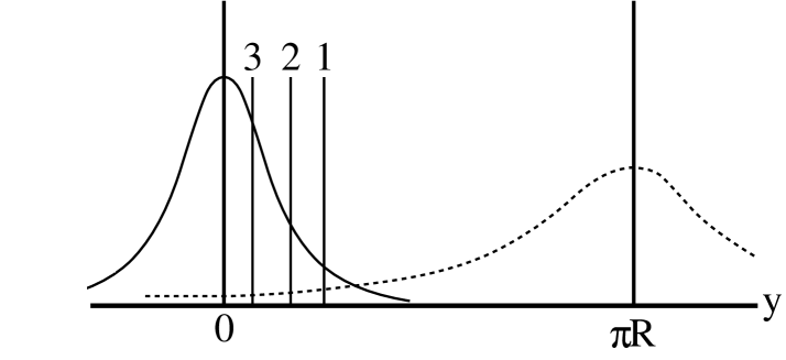
Figure 7: Schematic picture of the location of the matter fields. 1, 2 and 3 represents the location of the first, second and third generation of the matter fields. The solid line denotes the Higgs wave function and the dotted line denotes the wave function of NG fermion.

In the two-wall background configuration, SUSY is broken and fermion and sfermion masses split. Even though it is difficult to solve mass-eigenvalues directly, we can calculate the mass-splitting in each supermultiplet thanks to the low-energy theorem Eqs.(4.21) and (4.29). The overlap integral in Eq.(LABEL:overscalar) among the chiral supermultiplets localized on our wall and the NG fermion localized on the other wall determines the mass-splitting and hence sfermion masses. Thus the mass-eigenvalue of the sfermion becomes larger as the location is closer to the other wall.

Before estimating the sfermion mass spectrum, we comment on various scales in our theory. There are four typical scales in our theory: the five-dimensional Planck scale $M_{*}$, the compactification scale $(2\pi R)^{-1}$, the inverse width of the wall $\Lambda$ and the inverse width $a$ of zero-mode wave functions. In order for our setup to make sense, we had better keep the following relation among these scales

$$M_{*}>a>\Lambda>(2\pi R)^{-1}>5000~{}{\rm TeV}.$$ (5.3)

The inequality $a>\Lambda$ comes from the requirement that our wall must have enough width to trap matter modes. The last constraint is required to suppress flavor changing neutral currents mediated by Kaluza-Klein gauge bosons [26]. If we consider the flat background metric, $M_{*}$ and $R$ are related by the relation $M_{\rm pl}^{2}=(2\pi R)M_{*}^{3}$ where $M_{\rm pl}$ is the four-dimensional Planck scale. Thus the above constraint gives the lower bound for $M_{*}$, that is

$$M_{*}=\left(\frac{M_{\rm pl}^{2}}{2\pi R}\right)^{1/3}>\left(M_{\rm pl}^{2}\times 5000\mbox{TeV}\right)^{1/3}\simeq 8\times 10^{14}\mbox{GeV}.$$ (5.4)

Now, we would like to make a rough estimation of the gravity at the tree level by applying the results in section 4 and considering the scale $M$ as the five-dimensional Planck scale $M_{*}$. Let us start with the sfermion masses. We recall that the interaction Eq.(4.13) gives Yukawa coupling Eq.(4.20)

$$g_{{\rm eff}ij}=-\frac{1}{M_{*}^{3}}\int\!\!{\rm d}yF_{{\rm cl}}(y)f_{{\rm NG}}(y)b_{i,0}^{*}(y)f_{j,0}(y)\quad(i,j=1,2,3),$$ (5.5)

where we assumed ${\cal G}=\bar{\Phi}\Phi/M_{*}^{3}$ for simplicity. On the other hand, the low-energy theorem for the chiral supermultiplet (B.18) is

$$g_{{\rm eff}}=-\frac{\Delta m^{2}}{f}.$$ (5.6)

Assuming the fermion masses are small, we find that the sfermion masses are given by

$$(\tilde{m}^{2})_{ij} \!\!= \!\!\frac{f}{M_{*}^{3}}\int\!\!{\rm d}yF_{\rm cl}(y)f_{{\rm NG}}(y)b_{i,0}^{*}(y)f_{j,0}(y)$$ (5.7)

The classical configuration $A_{\rm cl}(y)$ is approximately linear in $y$ in the vicinity of the wall, and constant away from the wall. Correspondingly we can approximate $F_{{\rm cl}}(y)$ by a Gaussian function and the wave function of NG fermion by an exponential function, if we consider a large distance between two walls. We also adopt the Gaussian approximation for the zero-mode wave functions of the matter fields

$$b_{i,0}(y)\simeq f_{i,0}(y)\simeq N_{a}\exp[-a^{2}(y-y_{i})^{2}],$$ (5.8)

where $y_{i}$ is a location of the matter field and $a$ represents a typical inverse width and $N_{a}$ is a normalization constant of the zero-mode wave function for matter fields. Thus we obtain sfermion masses

$$(\tilde{m}^{2})_{ij} \!\!\simeq \!\!N_{a}^{2}\frac{f}{M_{*}^{3}}\int\!\!{\rm d}y~{}(\Lambda^{5/2}e^{-\Lambda^{2}y^{2}})~{}(\sqrt{\Lambda}e^{-\Lambda(\pi R-y)})~{}e^{-a^{2}(y-y_{i})^{2}}~{}e^{-a^{2}(y-y_{j})^{2}}$$ (5.9)

$$\!\!\simeq \!\!\frac{f}{\sqrt{2}}\left(\frac{\Lambda}{M_{*}}\right)^{3}\frac{{\rm Erf}~{}[\sqrt{2}\pi Ra]}{{\rm Erf}~{}[\pi Ra]}e^{-\Lambda\pi R}{\rm exp}\left[-\frac{a^{2}}{2}(y_{i}-y_{j})^{2}\right],$$ (5.10)

where the error function Erf [$x$] is defined as ${\rm Erf}~{}[x]\equiv\frac{2}{\sqrt{\pi}}\int^{x}_{0}dye^{-y^{2}}$ and the normalization constants $N_{a}^{2}=\frac{a}{\sqrt{\pi}{\rm Erf}~{}[\pi Ra]}$ are substituted. The approximation $2\pi R\gg y_{i}$ is used in the second line. One can see that the sfermion mass matrix is determined by only the relative difference of the coordinates where the matter fields are localized. The dependence of the distance between the location of the matter and the other wall is subleading. Using the typical example in Ref.[17] which well reproduces the fermion mass hierarchy and their mixings $y_{1}\sim 3.05M_{*}^{-1},y_{2}\sim 2.29M_{*}^{-1},y_{3}\sim 0.36M_{*}^{-1}$, and diagonalizing the sfermion mass matrix, we obtain the following results. If we consider the case $a\sim M_{*}$, the overlap between the wave functions of the different generations is small because the width of the wave function is small. Hence the hierarchy of the sfermion masses is at most one order of magnitude. On the other hand, if we consider the case $a\sim 0.1M_{*}$, the overlap between the wave functions of the different generations is larger, and all the matrix elements of sfermion mass squared matrix are nearly equal. In this case, the rank of the sfermion mass matrix is reduced, then the sfermion mass becomes ${\cal O}(10{\rm TeV}),{\cal O}(1{\rm TeV})$ and ${\cal O}(100{\rm GeV})$. Although this result looks like the decoupling solution [27] for FCNC problem, it has a mixing among the generations too large to be a viable solution for the FCNC problem. Since this result is an artifact of our rough approximation, we expect that a more realistic sfermion masses can be obtained, if we take account of flexibility of the model, such as the location and shape of the wave functions.

We now turn to the case of gaugino. Let us first consider the case that the gauge supermultiplet lives in the bulk. Eqs.(4.20) and (4.28) show that the overlap integral for the chiral supermultiplet receives an exponential suppression but that for the gauge supermultiplet does not. The gaugino tends to be heavier than the sfermions in this case. There are three ways to avoid this situation. One of them is to tune the numerical coefficient of the term Eq.(4.22) to be small. The second way is to localize the gauge supermultiplet on our wall. The third way is to assume that the function $\partial{\cal H}$ and $\partial^{c}{\cal H}$ in Eq.(4.30) have profiles which are localized on our wall. Then, even if the gauge supermultiplet lives in the bulk, the gaugino mass is suppressed because of the suppression of the overlap with the NG fermion localized on the other wall.

Next we consider the case that the gauge supermultiplet is localized on the wall. We also assume that the wave function of the zero mode of gauge supermultiplet is Gaussian

$$f_{\lambda_{1},0}(y)=b_{v,0}(y)\sim{\rm exp}(-a^{2}y^{2}).$$ (5.11)

Since Eq.(4.28) gives the gaugino mass through the low-energy theorem Eq.(4.29), we find by taking the limit $\pi R\gg\Lambda/(4a^{2})$

$$m_{\lambda} \!\!= \!\!\frac{f}{M_{*}^{3/2}}\int\!\!{\rm d}yf_{\lambda_{1},0}(y)f_{{\rm NG}}(y)b_{v,0}(y),$$ (5.12)

$$\!\!\simeq \!\!f\left(\frac{\Lambda}{2M_{*}^{3}}\right)^{1/2}{\rm exp}\left(-\Lambda\pi R+\frac{\Lambda^{2}}{8a^{2}}\right)\frac{{\rm Erf}~{}[\sqrt{2}\pi Ra]}{{\rm Erf}~{}[\pi Ra]},$$ (5.13)

where we assumed that the gauge kinetic function is ${\cal H}=\Phi/M^{3/2}$. Requiring $|m_{\lambda}|\sim{\cal O}(100$GeV), $\tilde{m}^{2}\sim{\cal O}({\rm TeV}^{2})$ and ${\rm exp}[-\frac{a^{2}}{2}(y_{i}-y_{j})^{2}]\simeq{\cal O}(0.1)\sim{\cal O}(1)$, we obtain

$$\Lambda\sim 10^{1.6\sim 2}\left({M_{*}\over{\rm GeV}}\right)^{3/5}{\rm GeV}.$$ (5.14)

Taking Eq.(5.3) into account, we obtain the bounds for $M_{*}$ and $\Lambda$

$$8\times 10^{14}~{}{\rm GeV}<M_{*}<3\times 10^{16}~{}{\rm GeV},$$ (5.15)

$$9\times 10^{10}~{}{\rm GeV}<\Lambda<3\times 10^{11}~{}{\rm GeV}.$$ (5.16)

SUSY breaking scale can be obtained from the gaugino mass as

$$\sqrt{f}\sim 2\times 10^{11}~{}{\rm GeV},$$ (5.17)

where we have used $\Lambda\sim 10^{11}~{}{\rm GeV}$ and $M_{*}\sim 10^{16}~{}{\rm GeV}$. SUSY breaking scale is comparable to that of the gravity mediation $\sqrt{f}\sim 10^{10\sim 11}$ GeV.

Finally, some comments are in order. The above Eqs.(5.10) and (5.13) include only effects of light modes at tree level of gravitational interaction. We would like to compare these gravity mediated contributions with those induced by coexisting walls ($M=\Lambda$). The bilinear term of the five-dimensional gravitino has a coefficient of order $c_{g}F_{\rm cl}(y)/M_{*}^{3/2}$ in the case of the gravity mediation, and of order $c_{w}F_{\rm cl}(y)/\Lambda^{3/2}$ in the case of coexisting walls, where $c_{g}$ and $c_{w}$ are numerical constants. As long as we have no information about the fundamental theory, we cannot calculate these constants $c_{g},c_{w}$ in the effective theory. Taking the ratio of these contributions, we obtain

$$\frac{\mbox{non-gravity}}{{\rm gravity}}\sim\frac{c_{w}}{c_{g}}\left(\frac{M_{*}}{\Lambda}\right)^{3/2}\sim\frac{c_{w}}{c_{g}}\left(\frac{10^{16}}{10^{11}}\right)^{3/2}\sim\frac{c_{w}}{c_{g}}\cdot 10^{7.5}.$$ (5.18)

If $c_{w}/c_{g}>10^{-7}$, the gravity mediated contribution is smaller than the non-gravity mediated contribution. If $c_{w}/c_{g}<10^{-8}$, the gravity mediated contribution is larger than the non-gravity mediated contribution.

The second comment is on the proton stability in our framework. In the “fat brane” approach, it is well known that the operators which are relevant to the proton decay are exponentially suppressed by separating the quark wave functions from the lepton wave functions [23]. This mechanism also works in our model. Noticing that the fifth dimension is compactified on a circle, it is sufficient for the wave functions of the quark and the lepton to be localized on the opposite side with respect to the plane $y=0$ where the Higgs field is localized. This relative location is required to reproduce the quark and lepton masses. Let us suppose that the distance between the locations of the quark and the lepton is $r$. Then, the dimension five operators are suppressed by $e^{-(ar)^{2}}/M_{*}=\frac{1}{M_{P}}\frac{M_{P}}{M_{*}}e^{-(ar)^{2}}$, where $M_{P}$ is the Planck scale in four dimensions. To keep the proton stable enough as required by experiments, $\frac{M_{P}}{M_{*}}e^{-(ar)^{2}}\sim 10^{-7}$ is needed. This constraint is indeed satisfied if we take $M_{*}\sim 10^{16}$ GeV and $ar\sim{\cal O}(\mbox{5 - 6})$, and is consistent with Eq.(5.3). Thus, the proton decay process is easily suppressed in our framework.

6 Discussion

In this paper, we proposed a simple SUSY breaking mechanism in the brane world scenario. The essence of our mechanism is just the coexistence of two different kinds of BPS domain walls at finite distance. Our mechanism needs no messenger fields nor complicated SUSY breaking sector on any of the walls. The low-energy theorem provides a powerful method to estimate the boson-fermion mass-splitting. Namely, the mass-splitting can be estimated by calculating an overlap integral of the mode functions for matter fields and the NG fermion. Matter fields are localized on our wall by definition. On the other hand, since the supersymmetry approximately preserved on our wall is broken due to the existence of the other wall, the corresponding NG fermion is localized on the other wall. Thus the mass-splitting induced in the effective theory is exponentially suppressed compared to the fundamental scale $\Lambda$. This is the generic feature of our mechanism.

Now let us discuss several further issues.

As mentioned below Eq.(2.22), the order parameter of the SUSY breaking $f$ is equal to the square root of the energy density of the wall $\sqrt{V_{0}}$. From the three-dimensional point of view, the fundamental theory is an ${\cal N}=2$ SUSY theory with $Q^{(1)}$- and $Q^{(2)}$-SUSYs. In general when a BPS domain wall exist, a half of the bulk SUSY, for example, $Q^{(2)}$-SUSY, is broken. In such a case, an order parameter of the SUSY breaking $f_{2}$ is equal to the square root of the energy density of the domain wall $\sqrt{V_{0}}$. However, if there is another BPS domain wall that breaks the other half of the bulk SUSY, $Q^{(1)}$-SUSY, there is another order parameter of the SUSY breaking $f_{1}$ and its square is expected to be equal to the energy density of the additional wall. In the model discussed in section 2, these two order parameters $f_{1}$ and $f_{2}$ are equal to each other. This is because the two walls are symmetric in this model. However in the case when our wall and the other wall are not symmetric, two order parameters $f_{1}$ and $f_{2}$ can have different values. In Appendix C, we discuss the possibility of such an asymmetric wall-configuration and the relation among $f_{1}$, $f_{2}$ and $V_{0}$ and central charge of the SUSY algebra.

If we try to construct a realistic model in our SUSY breaking mechanism, a fundamental bulk theory, which has a five-dimensional ${\cal N}=1$ SUSY, must have BPS domain walls. Since such a higher dimensional SUSY restricts the form of the superpotential severely, it is not easy to construct a BPS domain wall configuration. However, a BPS domain wall has been constructed in a four-dimensional ${\cal N}=2$ SUSY non-linear sigma model[28]. Since the nonlinear sigma model can be obtained from the ${\cal N}=1$ five-dimensional theory, this BPS domain wall can be regarded as a BPS domain wall that we desire. It is more difficult to obtain non-BPS configuration of two walls.

Our mechanism can be extended to higher dimensional cases straightforwardly. In such cases, our four-dimensional world is on various kinds of topological defects, such as vortices or intersections of domain walls in six dimensions, monopoles in seven dimensions, etc. Many higher dimensional theories have BPS configurations of these defects. Thus all we need for our mechanism is a stable non-BPS configuration corresponding to the coexistence of two or more BPS topological defects that preserve different parts of the bulk SUSY. We can always use the low-energy theorem like Eqs.(4.21) and (4.29) irrespective of the dimension of the bulk theory, in order to estimate the mass-splittings between bosons and fermions.

As a future work, we will investigate our SUSY breaking mechanism in the non-trivial metric like the Randall-Sundrum background [5]. To achieve this goal, we need to overcome the technical complexity of dealing with the five-dimensional supergravity. Besides, when we introduce the gravity, the size of the fifth dimension $2\pi R$ becomes a dynamical variable. In the model discussed in section 2, for example, the force between our wall and the other wall is repulsive. Thus the two-wall configuration Eq.(2.7) becomes unstable ($2\pi R$ goes to infinity) when the gravity is considered. So we must implement an extra mechanism to stabilize the two-wall configuration not only topologically but also under the gravity.

Acknowledgments

One of the authors (N.S.) is indebted to useful discussions with Kiwoon Choi, Takeo Inami, Ken-ichi Izawa, Martin Schmaltz, Tsutomu Yanagida, and Masahiro Yamaguchi. One of the authors (N.M.) thanks to a discussion with Hitoshi Murayama. This work is supported in part by Grant-in-Aid for Scientific Research from the Ministry of Education, Culture, Sports, Science and Technology,Japan, priority area(#707) “Supersymmetry and unified theory of elementary particles” and No.13640269. N.M.,Y.S. and R.S. are supported by the Japan Society for the Promotion of Science for Young Scientists (No.08557, No.10113 and No.6665).

Appendix A Low-energy theorem in three dimensions

In this appendix, we will review the low-energy theorem for the SUSY breaking briefly, and apply it to our mechanism.

A.1 SUSY Goldberger-Treiman relation

In general, when the supersymmetry is spontaneously broken, a massless fermion called the Nambu-Goldstone (NG) fermion $\psi_{\rm NG}(x)$ appears in the theory. It shows up in the supercurrent $J^{m}_{\alpha}(x)$ as follows[20]

$$J^{m}_{\alpha}=\sqrt{2}if\left(\gamma_{(3)}^{m}\psi_{\rm NG}\right)_{\alpha}+J^{m}_{\phi,\alpha}+\cdots,$$ (A.1)

where $f$ is the order parameter of the SUSY breaking and the abbreviation denotes higher order terms for $\psi_{\rm NG}(x)$. $J^{m}_{\phi,\alpha}(x)$ is the supercurrent for matter fields $\phi=(a,\psi)$ where $a(x)$ and $\psi(x)$ are a real scalar and a Majorana spinor fields respectively,

$$J^{m}_{\phi,\alpha}=\left(\gamma_{(3)}^{n}\gamma_{(3)}^{m}\psi\right)_{\alpha}\partial_{n}a+\cdots.$$ (A.2)

In the low-energy effective Lagrangian, there is a Yukawa coupling as follows.

$${\cal L}_{\rm Yukawa}=g_{{\rm eff}}a\psi\psi_{\rm NG}.$$ (A.3)

Here the effective coupling constant $g_{{\rm eff}}$ is related to the mass-splitting between the boson and the fermion $\Delta m^{2}\equiv m_{a}^{2}-m_{\psi}^{2}$ and the order parameter $f$ by[20]

$$g_{{\rm eff}}=\frac{\Delta m^{2}}{\sqrt{2}f}.$$ (A.4)

This is the supersymmetric analog of the Goldberger-Treiman relation.

A.2 Superpartners and mass-eigenstates

When SUSY is broken, a superpartner of a fermionic mass-eigenstate is not always a mass-eigenstate. In such a case, we should extend the formula Eq.(A.4) to more generic form.

Let us denote fermionic mass-eigenstates as $\psi_{1},\psi_{2},\cdots,\psi_{N}$, and their bosonic superpartners as $a_{1},a_{2},\cdots,a_{N}$. The bosonic mass-eigenstates $\tilde{a}_{1},\tilde{a}_{2},\cdots,\tilde{a}_{N}$ are related to $a_{1},a_{2},\cdots,a_{N}$ by

$$\left(\begin{array}[]{c}a_{1}\\ a_{2}\\ \vdots\\ a_{N}\end{array}\right)=V\left(\begin{array}[]{c}\tilde{a}_{1}\\ \tilde{a}_{2}\\ \vdots\\ \tilde{a}_{N}\end{array}\right),$$ (A.5)

where $V$ is an $N\times N$ unitary mixing matrix.

In this case, Eq.(A.4) is generalized to

$$g_{{\rm eff}i,j}=\frac{1}{\sqrt{2}f}\left(\Delta M^{2}\right)_{j,i},$$ (A.6)

where $g_{{\rm eff}i,j}$ are Yukawa coupling constants:

$${\cal L}_{\rm Yukawa}=\sum_{i,j}g_{{\rm eff}i,j}a_{i}\psi_{j}\psi_{\rm NG},$$ (A.7)

and $\Delta M^{2}$ is an $N\times N$ matrix defined by

$$\Delta M^{2}\equiv V\left(\begin{array}[]{ccc}m_{a_{1}}^{2}&&\\ &\ddots&\\ &&m_{a_{N}}^{2}\end{array}\right)-\left(\begin{array}[]{ccc}m_{\psi_{1}}^{2}&&\\ &\ddots&\\ &&m_{\psi_{N}}^{2}\end{array}\right)V.$$ (A.8)

A.3 Application to our model

To apply the above low-energy theorem to our mechanism of the SUSY breaking, we should interpret the four-(five-)dimensional bulk theory as a three-(four-)dimensional theory involving infinite Kaluza-Klein modes. To illustrate this, let us discuss the low-energy theorem by using the model Eq.(2.1) in the four-dimensional bulk as an example.

A.3.1 Three-dimensional super-transformation

The superpartner of $\psi^{(1)}_{p}(x)$ for $Q^{(1)}$-SUSY can be read off from the four-dimensional super-transformation,

$$\delta_{\xi}A(X)=\sqrt{2}\xi\Psi(X),$$ (A.9)

where $\xi$ is a Weyl spinor which parametrizes the super-transformation. By expanding the four-dimensional fields $A$ and $\Psi$ to infinite Kaluza-Klein modes like Eqs.(2.10), (2.13), (2.14), multiplying $f^{(1)}_{p}(y)$ and integrating in terms of $y$, we can obtain the three-dimensional super-transformation.

$$\delta_{\zeta}\sum_{q}\left\{\left(\int\!\!{\rm d}yf^{(1)}_{p}(y)b_{{\rm R},q}(y)\right)a_{{\rm R},q}(x)\right\}=\zeta\psi^{(1)}_{p}(x),$$ (A.10)

where $\zeta$ denotes the parameter of $Q^{(1)}$-transformation, which is a three-dimensional Majorana spinor.

Thus the superpartner of $\psi^{(1)}_{p}(x)$ for $Q^{(1)}$-SUSY, $a^{(1)}_{p}(x)$, is a linear combination of infinite mass-eigenmodes.

$$a^{(1)}_{p}(x)=\sum_{q}\left(\int\!\!{\rm d}yf^{(1)}_{p}(y)b_{{\rm R},q}(y)\right)a_{{\rm R},q}(x).$$ (A.11)

This is because $Q^{(1)}$-SUSY is broken by the background $A_{\rm cl}(y)$. When the distance between the walls is infinite, $Q^{(1)}$-SUSY is recovered and $a^{(1)}_{p}(x)$ becomes a mass-eigenmode. In this case, $Q^{(2)}$-SUSY is also recovered and $a^{(2)}_{p}(x)$, which is a superpartner of the mass-eigenmode $\psi^{(2)}_{p}(x)$, becomes a mass-eigenmode. Since the fields $a^{(1)}_{p}(x)$ and $a^{(2)}_{p}(x)$ are degenerate, they maximally mix when the wall distance is finite. For example,

$$\left(\begin{array}[]{c}a_{{\rm R},0}\\ a_{{\rm R},1}\end{array}\right)\simeq\frac{1}{\sqrt{2}}\left(\begin{array}[]{cc}1&-1\\ 1&1\end{array}\right)\left(\begin{array}[]{c}a^{(1)}_{0}\\ a^{(2)}_{0}\end{array}\right),$$ (A.12)

that is,

$$a^{(1)}_{0}\simeq\frac{1}{\sqrt{2}}\left(a_{{\rm R},0}+a_{{\rm R},1}\right).$$ (A.13)

This can be directly obtained from Eq.(A.11) by setting $p=0$.

Strictly speaking, $a^{(1)}_{0}(x)$ has slight but non-zero components of heavier fields $a_{{\rm R},p}(x)$ ($p\geq 2$). However these components become negligibly small as $p$ increases. Thus by introducing a cutoff $N$ for the Kaluza-Klein level and setting it large enough, we can apply the formula Eq.(A.6) to our case. The mixing matrix $V$ in Eq.(A.5) can be read off from Eq.(A.11) as follows.

$$V_{p,q}=\int\!\!{\rm d}yf^{(1)}_{p}(y)b_{{\rm R},q}(y).$$ (A.14)

A.3.2 Derivation of the formula Eq.(2.22)

Here we will derive the formula Eq.(2.22), as an example. Since the effective coupling constant $g_{{\rm eff}}$ in Eq.(2.18) is $g_{{\rm eff}1,0}$ in the notation here, it is related to the element $(\Delta M^{2})_{0,1}$ according to Eq.(A.6)

$$\left(\Delta M^{2}\right)_{0,1}=V_{0,1}m_{{\rm R},1},\quad V_{0,1}=\int\!\!{\rm d}yf^{(1)}_{0}(y)b_{{\rm R},1}(y)=k\frac{C_{0}}{C_{{\rm R},1}},$$ (A.15)

where normalization factors $C_{0}$ and $C_{{\rm R},1}$ are defined by Eq.(2.15) and Eq.(2.17), and

$$C_{0} \!\!= \!\!\left(\int\!\!{\rm d}y\left\{{\rm dn}\left(\frac{\Lambda y}{k},k\right)+k{\rm cn}\left(\frac{\Lambda y}{k},k\right)\right\}^{2}\right)^{-1/2}$$ (A.16)

$$\!\!= \!\!\left(\int\!\!{\rm d}y\left\{(1+k^{2})-2k^{2}{\rm sn}^{2}\left(\frac{\Lambda y}{k},k\right)\right\}\right)^{-1/2}=\left(V_{0}\frac{g^{2}k^{2}}{\Lambda^{4}}\right)^{-1/2}=\frac{\Lambda^{2}}{fgk}.$$

Here we used Eq.(2.19) and the relation $V_{0}=f^{2}$. Then we find the low-energy theorem Eq.(A.6) using Eq.(2.20)

$$\frac{1}{\sqrt{2}f}\left(\Delta M^{2}\right)_{0,1}=\frac{V_{0,1}m_{{\rm R},1}^{2}}{\sqrt{2}f}=\frac{1}{\sqrt{2}f}\cdot k\frac{C_{0}}{C_{{\rm R},1}}\cdot\frac{1-k^{2}}{k^{2}}\Lambda^{2}=\frac{g}{\sqrt{2}}\frac{C_{0}^{2}}{C_{{\rm R},1}}(1-k^{2})=g_{{\rm eff}}.$$ (A.17)

When the distance between the walls is large, $V_{0,1}\simeq 1/\sqrt{2}$ and we obtain Eq.(2.22).

In the above calculation, we assumed that the normalization factors $C_{0}$, $C_{{\rm R},0}$ and $C_{{\rm R},1}$ are all positive. In fact, we can calculate the boson-fermion mass-splittings including their sign, irrespective of the sign conventions of these normalization factors. Next, we will show this fact.

A.3.3 Unambiguity of the sign of the mass-splitting

Firstly, we should note that the sign of the normalization factor of the NG fermion $C_{0}$ is determined by the convention of the sign of the order parameter $f$.

The supercurrent in Eq.(A.1) can be obtained from that of the bulk theory,

$$J^{\mu}_{\alpha}=\sqrt{2}(\sigma^{\nu}\bar{\sigma}^{\mu}\Psi)_{\alpha}\partial_{\nu}A^{\ast}-i\sqrt{2}(\sigma^{\mu}\bar{\Psi})_{\alpha}\frac{\partial W^{\ast}}{\partial A^{\ast}}.$$ (A.18)

We define the three-dimensional currents $J^{(1)m}_{\alpha}(x)$ and $J^{(2)m}_{\alpha}(x)$ as follows.

$$\int\!\!{\rm d}yJ^{m}_{\alpha}(X)=\frac{1}{\sqrt{2}}\left(J^{(1)m}_{\alpha}(x)+iJ^{(2)m}_{\alpha}(x)\right),$$ (A.19)

where $J^{(1)m}_{\alpha}(x)$ and $J^{(2)m}_{\alpha}(x)$ are three-dimensional Majorana currents.

By substituting the mode expansion of fields:

$$A(x,y) \!\!= \!\!A_{\rm cl}(y)+\frac{1}{\sqrt{2}}\left\{\sum_{p}b_{{\rm R},p}(y)a_{{\rm R},p}(x)+i\sum_{p}b_{{\rm I},p}(y)a_{{\rm I},p}(x)\right\},$$

$$\Psi(x,y) \!\!= \!\!\frac{1}{\sqrt{2}}\left\{\sum_{p}f^{(1)}_{p}(y)\psi^{(1)}_{p}(x)+i\sum_{p}f^{(2)}_{p}(y)\psi^{(2)}_{p}(x)\right\},$$ (A.20)

into $J^{(1)m}_{\alpha}(x)$, we can obtain the three-dimensional supercurrent for $Q^{(1)}$-SUSY

$$J^{(1)m}(x) \!\!= \!\!\sqrt{2}i\left\{\int\!\!{\rm d}yf^{(2)}_{0}(y)\left(\partial_{y}A_{\rm cl}(y)-\frac{\Lambda^{2}}{g}\cos\left(\frac{g}{\Lambda}A_{\rm cl}(y)\right)\right)\right\}\gamma_{(3)}^{m}\psi^{(2)}_{0}(x)$$ (A.21)

$$\!\!+\sum_{p,q}V_{p,q}\gamma_{(3)}^{n}\gamma_{(3)}^{m}\psi^{(1)}_{p}(x)\partial_{n}a_{{\rm R},q}(x)+\cdots.$$

Comparing this to Eq.(A.1), we can see that the order parameter of the SUSY breaking $f$ is expressed by

$$f=\int\!\!{\rm d}yf^{(2)}_{0}(y)\left(\partial_{y}A_{\rm cl}(y)-\frac{\Lambda^{2}}{g}\cos\left(\frac{g}{\Lambda}A_{\rm cl}(y)\right)\right)=\frac{\Lambda^{2}}{gkC_{0}}.$$ (A.22)

Thus if we take a convention of $f>0$, the normalization factor $C_{0}$ is set to be positive.

Noticing that $(\Delta M^{2})_{p,q}=V_{p,q}(m_{{\rm R},q}^{2}-m_{p}^{2})$, we obtain the following formula from Eq.(A.6)

$$m_{{\rm R},q}^{2}-m_{p}^{2} \!\!= \!\!\sqrt{2}f\frac{g_{{\rm eff}q,p}}{V_{p,q}}$$ (A.23)

$$\!\!= \!\!\frac{\sqrt{2}\Lambda^{2}}{gkC_{0}}\frac{\int\!\!{\rm d}yb_{{\rm R},q}(y)f^{(1)}_{p}(y)f^{(2)}_{0}(y)}{\int\!\!{\rm d}yf^{(1)}_{p}(y)b_{{\rm R},q}(y)}.$$

Therefore we can calculate the mass-splitting $m_{{\rm R},q}^{2}-m_{p}^{2}$ including its sign, irrespective of the sign conventions of the normalization factors.

A.3.4 Estimation in the single-wall approximation

Finally, we comment on the estimation of the mass-splitting in the single-wall approximation (SWA). When we estimate the boson-fermion mass-splitting in SWA, we often approximate the bosonic mode function by that of its fermionic superpartner in the calculation of the overlap integral. This means that we estimate the following effective coupling as $g_{{\rm eff}ij}$ in Eq.(A.6).

$${\cal L}_{\rm Yukawa}=g_{{\rm eff}p}^{\rm(SWA)}a^{(1)}_{p}\psi^{(1)}_{p}\psi^{(2)}_{0}+\cdots.$$ (A.24)

As mentioned above, the superpartner $a^{(1)}_{p}(x)$ of the fermionic mass eigenmode $\psi^{(1)}_{p}(x)$ is a linear combination of mainly two bosonic mass-eigenmodes

$$a^{(1)}_{p}(x)\simeq\frac{1}{\sqrt{2}}(a_{{\rm R},2p}(x)+a_{{\rm R},2p+1}(x)).$$ (A.25)

Thus corresponding mode function $b^{(1)}_{p}(y)$ is

$$b^{(1)}_{p}(y)\simeq\frac{1}{\sqrt{2}}(b_{{\rm R},2p}(y)+b_{{\rm R},2p+1}(y)).$$ (A.26)

Then by using $b^{(1)}_{p}(y)$, which is well-approximated by $f^{(1)}_{p}(y)$, as a bosonic mode function, the formula Eq.(A.23) becomes

$$\sqrt{2}fg_{{\rm eff}p}^{\rm(SWA)} \!\!= \!\!\sqrt{2}f\int\!\!{\rm d}yb^{(1)}_{p}(y)f^{(1)}_{p}(y)f^{(2)}_{0}(y)$$ (A.27)

$$\!\!\simeq \!\!f\int\!\!{\rm d}y(b_{{\rm R},2p}(y)+b_{{\rm R},2p+1}(y))f^{(1)}_{p}(y)f^{(2)}_{0}(y)$$

$$\!\!\simeq \!\!f\frac{1}{\sqrt{2}}\left(\frac{g_{{\rm eff}2p,p}}{V_{2p,p}}+\frac{g_{{\rm eff}2p+1,p}}{V_{2p+1,p}}\right)$$

$$\!\!= \!\!\frac{1}{2}\left\{(m_{{\rm R},2p}^{2}-m_{p}^{2})+(m_{{\rm R},2p+1}^{2}-m_{p}^{2})\right\}$$

$$\!\!= \!\!\frac{m_{{\rm R},2p}^{2}+m_{{\rm R},2p+1}^{2}}{2}-m_{p}^{2},$$

where we used the fact that $V_{2p,p}\simeq V_{2p+1,p}\simeq 1/\sqrt{2}$, and the coupling constant $g_{{\rm eff}p}^{\rm(SWA)}$ is defined by

$$g_{{\rm eff}p}^{\rm(SWA)}\equiv\int\!\!{\rm d}yb^{(1)}_{p}(y)f^{(1)}_{p}(y)f^{(2)}_{0}(y)\simeq\int\!\!{\rm d}y\left(f^{(1)}_{p}(y)\right)^{2}f^{(2)}_{0}(y).$$ (A.28)

Therefore what we can estimate in the single-wall approximation is the difference between a fermionic mass and an average of squared masses of its bosonic superpartners.

Appendix B Low-energy theorem in four dimensions

In this appendix, we derive the low-energy theorem for chiral and gauge supermultiplets in four dimensions. We will follow the procedure in Ref.[20].

B.1 Low-energy theorem for Chiral supermultiplets

Let us denote one-particle state of a scalar boson with the mass $m_{\rm B}$ and the momentum $p_{\rm B}$ as $|p_{\rm B}\rangle$, and that of a spin 1/2 fermion with the mass $m_{\rm F}$ and the momentum $p_{\rm F}$ as $|p_{\rm F}\rangle$, which form a chiral supermultiplet. We perform the Lorentz decomposition of a matrix element for the supercurrent $J^{\mu}_{\alpha}(x)$ between these states.

$$\langle p_{\rm B}|J^{\mu}_{\alpha}(0)|p_{\rm F}\rangle \!\!= \!\![A_{1}(q^{2})q^{\mu}+A_{2}(q^{2})k^{\mu}+A_{3}(q^{2})\sigma^{\mu}\bar{\sigma}^{\nu}q_{\nu}]_{\alpha}^{\ \ \beta}\chi_{{\rm F}\beta}(p_{\rm F})$$ (B.1)

$$\!\!+[A_{4}(q^{2})\sigma^{\mu}+A_{5}(q^{2})q^{\mu}\sigma^{\nu}q_{\nu}+A_{6}(q^{2})k^{\mu}\sigma^{\nu}q_{\nu}]_{\alpha\dot{\beta}}\bar{\chi}_{\rm F}^{\ \dot{\beta}}(p_{\rm F}),$$

where $q^{\mu}\equiv p_{\rm B}^{\mu}-p_{\rm F}^{\mu}$ and $k^{\mu}\equiv p_{\rm B}^{\mu}+p_{\rm F}^{\mu}$. The spinors $\chi_{{\rm F}}(p_{\rm F})$ and $\bar{\chi}_{\rm F}^{\ }(p_{\rm F})$ obey the following equations

$$\sigma\cdot p_{\rm F}\bar{\chi}_{\rm F}^{\ }(p_{\rm F}) \!\!= \!\!m_{\rm F}\chi_{{\rm F}}(p_{\rm F}),\quad\bar{\sigma}\cdot p_{\rm F}\chi_{{\rm F}}(p_{\rm F})=m_{\rm F}\bar{\chi}_{\rm F}^{\ }(p_{\rm F}).$$ (B.2)

Conservation of the supercurrent leads to a relation among the form factors as

$$q^{2}\left[A_{1}(q^{2})-A_{3}(q^{2})\right]=\Delta m^{2}A_{2}(q^{2}),$$ (B.3)

where $\Delta m^{2}\equiv m_{\rm B}^{2}-m_{\rm F}^{2}$ is a mass-splitting between the boson and the fermion.

To discuss S-matrix elements, we define an NG fermion source $j^{\rm NG}_{\alpha}(x)$ by using the NG fermion field $\psi_{\rm NG}(x)$ as

$$j^{\rm NG}_{\alpha}(x)=-i\sigma^{\mu}_{\alpha\dot{\alpha}}\partial_{\mu}\bar{\psi}_{\rm NG}^{\dot{\alpha}}(x).$$ (B.4)

Its matrix element between the boson and the fermion states is decomposed as

$$\langle p_{\rm B}|j^{\rm NG}_{\alpha}(0)|p_{\rm F}\rangle=B_{1}(q^{2})\chi_{{\rm F}\alpha}(p_{\rm F})+B_{2}(q^{2})q\cdot\sigma_{\alpha\dot{\alpha}}\bar{\chi}_{\rm F}^{\ \dot{\alpha}}(p_{\rm F}),$$ (B.5)

and thus

$$\langle p_{\rm B}|\bar{\psi}_{\rm NG}^{\dot{\alpha}}(0)|p_{\rm F}\rangle=-\frac{B_{1}(q^{2})}{q^{2}}q\cdot\bar{\sigma}^{\dot{\alpha}\alpha}\chi_{{\rm F}\alpha}(p_{\rm F})+B_{2}(q^{2})\bar{\chi}_{\rm F}^{\ \dot{\alpha}}(p_{\rm F}).$$ (B.6)

Since the combination $J^{\mu}_{\alpha}-\sqrt{2}if\sigma^{\mu}_{\alpha\dot{\alpha}}\bar{\psi}_{\rm NG}^{\dot{\alpha}}$ has vanishing matrix element between the vacuum and the single NG fermion state, all the form factors of $\langle p_{\rm B}|J^{\mu}_{\alpha}-\sqrt{2}if\sigma^{\mu}_{\alpha\dot{\alpha}}\bar{\psi}_{\rm NG}^{\dot{\alpha}}|p_{\rm F}\rangle$ are regular as $q^{2}\to 0$. Then comparing Eqs.(B.1) and (B.6), we can see that the form factor $A_{3}(q^{2})$ is singular at $q^{2}=0$ unless $B_{1}(0)$ is zero.

$$\lim_{q^{2}\to 0}q^{2}A_{3}(q^{2})=-\sqrt{2}ifB_{1}(0).$$ (B.7)

Substituting it into Eq.(B.3) with the limit $q^{2}\to 0$, we obtain

$$\sqrt{2}ifB_{1}(0)=\Delta m^{2}A_{2}(0).$$ (B.8)

To relate the form factor $B_{1}(0)$ to an effective coupling constant of the NG fermion with the boson and the fermion forming a chiral supermultiplet, we evaluate a transition amplitude between the in-state $|q;p_{\rm F}\rangle_{\rm in}$ and the out-state $|p_{\rm B}\rangle_{\rm out}$. This S-matrix element can be expressed by using an effective interaction Lagrangian ${\cal L}_{\rm int}$ as

$$\mbox{}_{\rm out}\langle p_{\rm B}|q;p_{\rm F}\rangle_{\rm in} \!\!= \!\!\mbox{}_{\rm I}\langle p_{\rm B}|e^{i\int\!\!{\rm d}^{4}x{\cal L}_{\rm int}(x)}|p_{\rm F}\rangle_{\rm I}$$ (B.9)

$$\!\!\simeq \!\!i(2\pi)^{4}\delta^{4}(p_{\rm B}-p_{\rm F}-q)\>\mbox{}_{\rm I}\langle p_{\rm B}|{\cal L}_{\rm int}(0)|q;p_{\rm F}\rangle_{\rm I},$$

where $|p_{\rm B}\rangle_{\rm I}$ and $|q;p_{\rm F}\rangle_{\rm I}$ denote states in the interaction picture.

On the other hand, using the LSZ reduction formula, it can also be written as

$$\mbox{}_{\rm in}\langle p_{\rm B}|q;p_{\rm F}\rangle_{\rm out} \!\!= \!\!-i(2\pi)^{4}\delta^{4}(p_{\rm B}-p_{\rm F}-q)\chi_{\rm NG}(q)q_{\mu}\sigma^{\mu}\mbox{}_{\rm I}\langle p_{\rm B}|\bar{\psi}_{\rm NG}(0)|p_{\rm F}\rangle_{\rm I}$$ (B.10)

$$\!\!-i(2\pi)^{4}\delta^{4}(p_{\rm B}-p_{\rm F}-q)\bar{\chi}_{\rm NG}(q)q_{\mu}\bar{\sigma}^{\mu}\mbox{}_{\rm I}\langle p_{\rm B}|\psi_{\rm NG}(0)|p_{\rm F}\rangle_{\rm I},$$

where $\chi_{\rm NG}(q)$ and $\bar{\chi}_{\rm NG}(q)$ are the NG fermion spinors. Since we do not need to distinguish the interaction picture and the Heisenberg picture for one-particle states, we drop the subscript I for one-particle states in the following. We obtain a relation between matrix elements of the interaction Lagrangian and the NG fermion field

$$\langle p_{\rm B}|{\cal L}_{\rm int}(0)|q;p_{\rm F}\rangle_{\rm I}=-\chi_{\rm NG}(q)q_{\mu}\sigma^{\mu}\langle p_{\rm B}|\bar{\psi}_{\rm NG}(0)|p_{\rm F}\rangle-\bar{\chi}_{\rm NG}(q)q_{\mu}\bar{\sigma}^{\mu}\langle p_{\rm B}|\psi_{\rm NG}(0)|p_{\rm F}\rangle.$$ (B.11)

At soft NG fermion limit $q^{\mu}\to 0$, the S-matrix element Eq.(B.9) should be expressible by the following nonderivative interaction terms in the effective Lagrangian [19]

$${\cal L}_{\rm int}=g_{{\rm eff}}a^{*}\psi\psi_{\rm NG}+{\rm h.c.}+\cdots,$$ (B.12)

where $a$ is a complex scalar field and $\psi$ is a two-component Weyl spinor field, which create or annihilate the states $|p_{\rm B}\rangle$ and $|p_{\rm F}\rangle$ respectively. So its matrix element is written as

$$\langle p_{\rm B}|{\cal L}_{\rm int}(0)|q;p_{\rm F}\rangle_{\rm I}=g_{{\rm eff}}\chi_{\rm NG}(q)\chi_{{\rm F}}(p_{\rm F})+g_{{\rm eff}}\bar{\chi}_{\rm NG}(q)\bar{\chi}_{\rm F}^{\ }(p_{\rm F}).$$ (B.13)

Substituting Eq.(B.6) into Eq.(B.11), and comparing it with Eq.(B.13) gives a relation between $B_{1}(0)$ and $g_{{\rm eff}}$

$$B_{1}(0)=-g_{{\rm eff}}.$$ (B.14)

Thus Eq.(B.8) becomes the supersymmetric analog of the Goldberger-Treiman relation

$$\sqrt{2}g_{{\rm eff}}f=i(m_{\rm B}^{2}-m_{\rm F}^{2})A_{2}(0).$$ (B.15)

Noting that the supercurrent takes the form

$$J^{\mu}_{\alpha}=\sqrt{2}if\sigma^{\mu}_{\alpha\dot{\alpha}}\bar{\psi}_{\rm NG}^{\dot{\alpha}}+\sqrt{2}\left(\sigma^{\nu}\bar{\sigma}^{\mu}\psi\right)_{\alpha}\partial_{\nu}a^{*}+\cdots,$$ (B.16)

and substituting it into the left-hand-side of Eq.(B.1) with the limit $q^{2}\to 0$, we can determine the value of the form factor $A_{2}(0)$ as

$$A_{2}(0)=\sqrt{2}i.$$ (B.17)

Thus we obtain the low-energy theorem for the chiral supermultiplets from Eq.(B.15)

$$g_{{\rm eff}}=-\frac{m_{\rm B}^{2}-m_{\rm F}^{2}}{f}.$$ (B.18)

B.2 Low-energy theorem for Gauge supermultiplets

Next we derive the low-energy theorem for gauge supermultiplets. As the case of chiral supermultiplets, we consider the Lorentz decomposition of the matrix element for the supercurrent $J^{\mu}_{\alpha}(x)$ between one-particle state of the gauge boson $|p_{\rm B}\rangle$ with the mass $m_{\rm B}$ and the momentum $p_{\rm B}$, and that of the gaugino $|p_{\rm F}\rangle$ with the mass $m_{\rm F}$ and the momentum $p_{\rm F}$

$$\begin{array}[]{l}\langle p_{\rm B}|J^{\mu}_{\alpha}(0)|p_{\rm F}\rangle\vspace{1mm}\\ \ \ \ =\ \epsilon^{\ast}_{\nu}(p_{\rm B})\bigl{[}A_{1}(q^{2})q^{\nu}q^{\mu}+A_{2}(q^{2})q^{\nu}k^{\mu}+A_{3}(q^{2})q^{\nu}\sigma^{\mu}\bar{\sigma}^{\rho}q_{\rho}+A_{4}(q^{2})\eta^{\mu\nu}+A_{5}(q^{2})\sigma^{\nu}\bar{\sigma}^{\mu}\bigr{]}_{\alpha}^{\ \ \beta}\chi_{{\rm F}\beta}(p_{\rm F})\vspace{1mm}\\ \ \ \ \ +\ \epsilon^{\ast}_{\nu}(p_{\rm B})\bigl{[}A_{6}(q^{2})q^{\nu}\sigma^{\mu}+A_{7}(q^{2})q^{\nu}q^{\mu}\sigma^{\rho}q_{\rho}+A_{8}(q^{2})q^{\nu}k^{\mu}\sigma^{\rho}q_{\rho}+A_{9}(q^{2})\eta^{\mu\nu}\sigma^{\rho}q_{\rho}\vspace{1mm}\\ \hskip 142.26378pt+A_{10}(q^{2})q^{\mu}\sigma^{\nu}+A_{11}(q^{2})\sigma^{\nu}\bar{\sigma}^{\rho}\sigma^{\mu}k_{\rho}+A_{12}(q^{2})\sigma^{\mu}\bar{\sigma}^{\rho}\sigma^{\nu}q_{\rho}\bigr{]}_{\alpha\dot{\beta}}\bar{\chi}_{\rm F}^{\ \dot{\beta}}(p_{\rm F}),\end{array}$$ (B.19)

where $q^{\mu}=p_{\rm B}^{\mu}-p_{\rm F}^{\mu}$, $k^{\mu}=p_{\rm B}^{\mu}+p_{\rm F}^{\mu}$ and $\epsilon^{\ast}_{\nu}(p_{\rm B})$ is a polarization vector with $p_{\rm B}\cdot\epsilon^{\ast}(p_{\rm B})=0$.

Conservation of the supercurrent leads to a relation among the form factors

$$q^{2}\left[A_{10}(q^{2})+A_{11}(q^{2})-A_{12}(q^{2})\right]=-2\Delta m^{2}A_{11}(q^{2}),$$ (B.20)

where $\Delta m^{2}\equiv m_{\rm B}^{2}-m_{\rm F}^{2}$ is the mass-splitting between the gauge boson and the gaugino.

A matrix element of the NG fermion source $j^{\rm NG}_{\alpha}(x)$ between the gauge boson and the gaugino states are decomposed as

$$\langle p_{\rm B}|j_{\alpha}^{\rm NG}(0)|p_{\rm F}\rangle\ =\ \epsilon^{\ast}_{\nu}(p_{\rm B})\left[B_{1}(q^{2})q^{\nu}+B_{2}(q^{2})q_{\rho}\sigma^{\rho}\bar{\sigma}^{\nu}\right]_{\alpha}^{\ \ \beta}\chi_{{\rm F}\beta}(p_{\rm F})\vspace{1mm}$$

$$\hskip 142.26378pt+\ \epsilon^{\ast}_{\nu}(p_{\rm B})\left[B_{3}(q^{2})q^{\nu}\sigma^{\rho}q_{\rho}+B_{4}(q^{2})\sigma^{\nu}\right]_{\alpha\dot{\beta}}\bar{\chi}_{\rm F}^{\ \dot{\beta}}(p_{\rm F}),$$ (B.21)

and thus

$$\langle p_{\rm B}|\bar{\psi}_{\rm NG}^{\dot{\alpha}}(0)|p_{\rm F}\rangle\ =\ \epsilon^{\ast}_{\nu}(p_{\rm B})\left[-\displaystyle{\frac{B_{1}(q^{2})}{q^{2}}}q^{\nu}\bar{\sigma}^{\rho}q_{\rho}+B_{2}(q^{2})\bar{\sigma}^{\nu}\right]^{\dot{\alpha}\beta}\chi_{{\rm F}\beta}(p_{\rm F})\vspace{1mm}$$

$$\hskip 142.26378pt+\ \epsilon^{\ast}_{\nu}(p_{\rm B})\left[B_{3}(q^{2})q^{\nu}-\displaystyle{\frac{B_{4}(q^{2})}{q^{2}}}q_{\rho}\bar{\sigma}^{\rho}\sigma^{\nu}\right]^{\dot{\alpha}}_{\ \ \dot{\beta}}\bar{\chi}_{\rm F}^{\ \dot{\beta}}(p_{\rm F}).$$ (B.22)

The regularity of the form factors of the matrix element for $J^{\mu}_{\alpha}-\sqrt{2}if\sigma^{\mu}_{\alpha\dot{\alpha}}\bar{\psi}_{\rm NG}^{\dot{\alpha}}$ as $q^{2}\to 0$ leads to the singularity of the form factor $A_{12}(q^{2})$ at $q^{2}=0$

$$\lim_{q^{2}\to 0}q^{2}A_{12}(q^{2})=-\sqrt{2}ifB_{4}(0).$$ (B.23)

Substituting it into Eq.(B.20) with the limit $q^{2}\to 0$, we obtain

$$\sqrt{2}ifB_{4}(0)=-2\Delta m^{2}A_{11}(0).$$ (B.24)

We can relate the form factor $B_{4}(0)$ to an effective coupling constant of the NG fermion with the gauge boson and the gaugino forming a gauge supermultiplet. By repeating the same procedure as that in the previous subsection leading to Eq.(B.11), we obtain

$$\langle p_{\rm B}|{\cal L}_{\rm int}(0)|q;p_{\rm F}\rangle_{\rm I}=-\chi_{\rm NG}(q)q_{\mu}\sigma^{\mu}\langle p_{\rm B}|\bar{\psi}_{\rm NG}(0)|p_{\rm F}\rangle-\bar{\chi}_{\rm NG}(q)q_{\mu}\bar{\sigma}^{\mu}\langle p_{\rm B}|\psi_{\rm NG}(0)|p_{\rm F}\rangle.$$ (B.25)

On the other hand, we expect the following nonderivative interaction terms in the effective Lagrangian[19]

$${\cal L}_{\rm int}=h_{{\rm eff}}\psi_{\rm NG}\sigma^{\mu\nu}\lambda v_{\mu\nu}+{\rm h.c.}+\cdots,$$ (B.26)

where $\lambda$ is the gaugino field and $v_{\mu\nu}$ is the gauge field strength respectively. So its matrix element is written as

$$\langle p_{\rm B}|{\cal L}_{\rm int}(0)|q;p_{\rm F}\rangle_{\rm I}=ih_{{\rm eff}}\epsilon^{\ast}_{\nu}(p_{\rm B})p_{{\rm B}\mu}\chi_{\rm NG}(q)\sigma^{\nu}\bar{\sigma}^{\mu}\chi_{{\rm F}}(p_{\rm F})+ih_{{\rm eff}}\epsilon^{\ast}_{\nu}(p_{\rm B})p_{{\rm B}\mu}\bar{\chi}_{\rm NG}(q)\bar{\sigma}^{\nu}\sigma^{\mu}\bar{\chi}_{\rm F}^{\ }(p_{\rm F}).$$ (B.27)

For the case of $m_{\rm F}\neq 0$, comparison between Eq.(B.25) and Eq.(B.27) after substitution of Eq.(B.22) into Eq.(B.25) gives

$$B_{4}(0)=-im_{\rm F}h_{{\rm eff}}.$$ (B.28)

Using Eq.(B.24) we obtain the analog of the Goldberger-Treiman relation for gauge supermultiplets

$$-\sqrt{2}h_{{\rm eff}}f=\frac{2(m_{\rm B}^{2}-m_{\rm F}^{2})}{m_{\rm F}}A_{11}(0).$$ (B.29)

To determine the form factor $A_{11}(0)$, we substitute the following expression of the supercurrent into Eq.(B.19) with the limit $q^{2}\to 0$.

$$J^{\mu}_{\alpha}=\sqrt{2}if\sigma^{\mu}_{\alpha\dot{\alpha}}\bar{\psi}_{\rm NG}^{\dot{\alpha}}-iv_{\nu\rho}\left(\sigma^{\nu\rho}\sigma^{\mu}\right)_{\alpha\dot{\alpha}}\bar{\lambda}^{\dot{\alpha}}+\cdots\ .$$ (B.30)

Then we find

$$A_{11}(0)=\frac{1}{2}.$$ (B.31)

By substituting it into Eq.(B.29), we obtain the low-energy theorem for the gauge supermultiplets

$$h_{{\rm eff}}=-\frac{1}{\sqrt{2}f}\left(\frac{m_{\rm B}^{2}}{m_{\rm F}}-m_{\rm F}\right).$$ (B.32)

Appendix C Relation among central charge and order parameters

In the single-wall case, the order parameter $f$ for the SUSY breaking due to the existence of a BPS domain wall is given by the square root of the energy density of the wall $\sqrt{V_{0}}$. In the two-wall system, however, two different SUSY breakings occur, whose origins are our wall and the other wall respectively. Thus there are in general two kinds of order parameters $f_{1}$ and $f_{2}$ for different SUSY breakings. Here we shall clarify the relation among $f_{1}$, $f_{2}$ and $V_{0}$ and the central charge of the SUSY algebra.

Let us begin with the four-dimensional SUSY algebra of the bulk theory. Since we consider the case of the SUSY breaking, we describe the SUSY algebra in the local form. The three-dimensional SUSY algebra can be derived from the four-dimensional one with the central charge:

$$\left\{Q_{\alpha},\bar{J}^{\nu}_{\dot{\beta}}(X)\right\} \!\!= \!\!2\sigma^{\mu}_{\alpha\dot{\beta}}T_{\mu}^{\ \nu}(X),$$ (C.1)

$$\left\{Q_{\alpha},J^{\nu}_{\beta}(X)\right\} \!\!= \!\!4i\left(\sigma^{\mu}\bar{\sigma}^{\nu}\right)_{\alpha}^{\ \gamma}\epsilon_{\gamma\beta}\partial_{\mu}W^{*}(A^{*}(X)),$$ (C.2)

where $T_{\mu}^{\ \nu}(X)$ is the energy-momentum tensor

$$T_{\mu}^{\ \nu}=\partial^{\nu}A^{*}\partial_{\mu}A+\partial^{\nu}A\partial_{\mu}A^{*}+\frac{i}{2}\bar{\Psi}\bar{\sigma}^{\nu}\partial_{\mu}\Psi+\frac{i}{2}\Psi\sigma^{\nu}\partial_{\mu}\bar{\Psi}+\delta_{\mu}^{\ \nu}{\cal L}$$ (C.3)

The term containing the superpotential $W(\Phi)$ represents the density of the central charge. In this section, we calculate the SUSY algebra in the following Wess-Zumino model for simplicity.

$${\cal L}=\left.\bar{\Phi}\Phi\right|_{\theta^{2}\bar{\theta}^{2}}+\left.W(\Phi)\right|_{\theta^{2}}+{\rm h.c.},$$ (C.4)

where $\Phi=A+\sqrt{2}\theta\Psi+\theta^{2}F$ is a chiral superfield.

Eqs.(C.1) and (C.2) can be rewritten in terms of the three-dimensional supercurrent defined by Eq.(A.19) as

$$\left\{Q^{(1)}_{\alpha},J^{(1)n\beta}(x)\right\} \!\!= \!\!2\left(\gamma_{(3)}^{m}\right)_{\alpha}^{\ \beta}\left(Y_{m}^{\ n}-2\delta_{m}^{\ n}\Delta W^{*}\right),$$ (C.5)

$$\left\{Q^{(2)}_{\alpha},J^{(2)n\beta}(x)\right\} \!\!= \!\!2\left(\gamma_{(3)}^{m}\right)_{\alpha}^{\ \beta}\left(Y_{m}^{\ n}+2\delta_{m}^{\ n}\Delta W^{*}\right),$$ (C.6)

$$\left\{Q^{(1)}_{\alpha},J^{(2)n}_{\beta}(x)\right\} \!\!= \!\!2\epsilon_{\alpha\beta}Y_{2}^{\ n},$$ (C.7)

$$\left\{Q^{(2)}_{\alpha},J^{(1)n}_{\beta}(x)\right\} \!\!= \!\!-2\epsilon_{\alpha\beta}Y_{2}^{\ n},$$ (C.8)

where

$$Y_{\mu}^{\ \nu}(x)\equiv\int\!\!{\rm d}yT_{\mu}^{\ \nu}(X),\;\;\;\Delta W\equiv\int\!\!{\rm d}y\partial_{y}W(A(X)).$$ (C.9)

Note that $\Delta W$ is constant since it depends only on the boundary condition along the extra dimension and becomes non-zero on a non-trivial boundary condition. Here we suppose that the background configuration $A_{\rm cl}(y)$ is real, for simplicity. Thus the central charge $\Delta W$ is treated as a real constant in the following discussion.

Since the background $A_{\rm cl}(y)$ is real, four-dimensional fields $A(X)$ and $\Psi(X)$ are mode-expanded as follows.

$$A(X) \!\!= \!\!A_{\rm cl}(y)+\frac{1}{\sqrt{2}}\left(\sum_{p=0}^{\infty}b_{{\rm R},p}(y)a_{{\rm R},p}(x)+i\sum_{p=1}^{\infty}b_{{\rm I},p}(y)a_{{\rm I},p}(x)\right),$$ (C.10)

$$\Psi(X) \!\!= \!\!\frac{1}{\sqrt{2}}\left(\sum_{p=0}^{\infty}f^{(1)}_{p}(y)\psi^{(1)}_{p}(x)+i\sum_{p=0}^{\infty}f^{(2)}_{p}(y)\psi^{(2)}_{p}(x)\right).$$ (C.11)

Note the NG boson $a_{{\rm R},0}(x)$ for the broken translational invariance along the extra dimension comes from the real part of $A(x)$ because $A_{\rm cl}(y)$ is real. In the fermionic sector, there are the NG fermions $\psi^{(2)}_{0}(x)$ and $\psi^{(1)}_{0}(x)$ for broken $Q^{(1)}$- and $Q^{(2)}$-SUSY, respectively.

$Y_{\mu}^{\ \nu}(x)$ can be rewritten in terms of three-dimensional fields as

$$Y_{m}^{\ n}(x) \!\!= \!\!-\delta_{m}^{\ n}V_{0}+\sum_{p=0}^{\infty}\partial^{n}a_{{\rm R},p}\partial_{m}a_{{\rm R},p}+\sum_{p=1}^{\infty}\partial^{n}a_{{\rm I},p}\partial_{m}a_{{\rm I},p}$$ (C.12)

$$\!\!+\frac{i}{2}\sum_{p=0}^{\infty}\psi^{(1)}_{p}\gamma_{(3)}^{n}\partial_{m}\psi^{(1)}_{p}+\frac{i}{2}\sum_{p=0}^{\infty}\psi^{(2)}_{p}\gamma_{(3)}^{n}\partial_{m}\psi^{(2)}_{p}+\delta_{m}^{\ n}{\cal L}^{(3)}$$

$$\!\!= \!\!-\delta_{m}^{\ n}V_{0}+T_{(3)m}^{\ \ \ \ n}(x),$$ (C.13)

$$Y_{2}^{\ m}(x) \!\!= \!\!f_{\rm P}\partial^{m}a_{{\rm R},0}+\cdots,$$ (C.14)

where $V_{0}$ is the energy density of the background

$$V_{0}\equiv\int\!\!{\rm d}y\left\{(\partial_{y}A_{\rm cl})^{2}+\left|\frac{\partial W}{\partial A}\right|^{2}_{A=A_{\rm cl}}\right\},$$ (C.15)

and $T_{(3)m}^{\ \ \ \ n}(x)$ is the three-dimensional energy-momentum tensor. $f_{\rm P}$ in Eq.(C.14) corresponds an order parameter for the breaking of the translational invariance along the extra dimension

$$f_{\rm P}=\sqrt{2}\int\!\!{\rm d}yb_{{\rm R},0}(y)\partial_{y}A_{\rm cl}(y).$$ (C.16)

Then, the three-dimensional SUSY algebra becomes as follows.

$$\left\{Q^{(1)}_{\alpha},J^{(1)n\beta}(x)\right\} \!\!= \!\!2\left(\gamma_{(3)}^{m}\right)_{\alpha}^{\ \beta}\left\{-\delta_{m}^{\ n}(V_{0}+2\Delta W)+T_{(3)m}^{\ \ \ \ n}\right\},$$ (C.17)

$$\left\{Q^{(2)}_{\alpha},J^{(2)n\beta}(x)\right\} \!\!= \!\!2\left(\gamma_{(3)}^{m}\right)_{\alpha}^{\ \beta}\left\{-\delta_{m}^{\ n}(V_{0}-2\Delta W)+T_{(3)m}^{\ \ \ \ n}\right\},$$ (C.18)

$$\left\{Q^{(1)}_{\alpha},J^{(2)n}_{\beta}(x)\right\} \!\!= \!\!2\epsilon_{\alpha\beta}\left(f_{\rm P}\partial^{n}a_{{\rm R},0}+\cdots\right),$$ (C.19)

$$\left\{Q^{(2)}_{\alpha},J^{(1)n}_{\beta}(x)\right\} \!\!= \!\!2\epsilon_{\beta\alpha}\left(f_{\rm P}\partial^{n}a_{{\rm R},0}+\cdots\right).$$ (C.20)

On the other hand, the supercurrents have the following forms

$$J^{(1)m}_{\alpha}=\sqrt{2}if_{1}\left(\gamma_{(3)}^{m}\psi^{(2)}_{0}\right)_{\alpha}+\cdots,\;\;\;J^{(2)m}_{\alpha}=\sqrt{2}if_{2}\left(\gamma_{(3)}^{m}\psi^{(1)}_{0}\right)_{\alpha}+\cdots,$$ (C.21)

where $f_{1}$ and $f_{2}$ are the order parameters of the breaking for $Q^{(1)}$- and $Q^{(2)}$-SUSY respectively.

Then using the commutation relation of the three-dimensional Majorana spinors

$$\left\{\psi_{\alpha}(\vec{x},t),\psi_{\beta}(\vec{x}^{\prime},t)\right\}=-\left(\gamma_{(3)}^{0}\sigma^{2}\right)_{\alpha\beta}\delta^{2}(\vec{x}-\vec{x}^{\prime}),$$ (C.22)

Eqs.(C.17) and (C.18) are also written as

$$\left\{Q^{(1)}_{\alpha},J^{(1)n\beta}(x)\right\} \!\!= \!\!-2f_{1}^{2}\left(\gamma_{(3)}^{n}\right)_{\alpha}^{\ \beta}+\cdots,$$ (C.23)

$$\left\{Q^{(2)}_{\alpha},J^{(2)n\beta}(x)\right\} \!\!= \!\!-2f_{2}^{2}\left(\gamma_{(3)}^{n}\right)_{\alpha}^{\ \beta}+\cdots.$$ (C.24)

By comparing these commutation relations with Eqs.(C.17) and (C.18), we obtain the following relations

$$V_{0}=\frac{f_{1}^{2}+f_{2}^{2}}{2},\;\;\;\Delta W=\frac{f_{1}^{2}-f_{2}^{2}}{4}.$$ (C.25)

Thus the average of the squares of two different kinds of order parameters gives the energy density of the background and their difference gives the central charge. From the second relation in Eq.(C.25), we can conclude that if the extra dimension is compactified, the superpotential $W$ must be a multi-valued function, such as those in Ref.[29], in order to realize a situation where the order parameter for the breaking of the $Q^{(1)}$-SUSY is different from that of the $Q^{(2)}$-SUSY.

References

- [1] S. Dimopoulos and H. Georgi, Nucl. Phys. B193 (1981) 150; N. Sakai, Z. f. Phys. C11 (1981) 153; E. Witten, Nucl. Phys. B188 (1981) 513; S. Dimopoulos, S. Raby, and F. Wilczek, Phys. Rev. D24 (1981) 1681.
- [2] A. Chamseddine, R. Arnowitt, and P. Nath, Phys. Rev. Lett. 49 (1982) 970; R. Barbieri, S. Ferrara, and C. Savoy, Phys. Lett. B119 (1982) 334; L. Hall, J. Lykken and S. Weinberg, Phys. Rev. D27 (1983) 2359.
- [3] M. Dine and A. Nelson, Phys. Rev. D48 (1993) 1277 [hep-ph/9303230]; M. Dine, A. Nelson, and Y. Shirman, Phys. Rev. D51 (1995) 1362 [hep-ph/9408384]; M. Dine, A. Nelson, Y. Nir, and Y. Shirman, Phys. Rev. D53 (1996) 2658 [hep-ph/9507378].
- [4] N. Arkani-Hamed, S. Dimopoulos and G. Dvali, Phys. Lett. B429 (1998) 263 [hep-ph/9803315]; I. Antoniadis, N. Arkani-Hamed, S. Dimopoulos and G. Dvali, Phys. Lett. B436 (1998) 257 [hep-ph/9804398].
- [5] L. Randall and R. Sundrum, Phys. Rev. Lett. 83 (1999) 3370 [hep-ph/9905221]; Phys. Rev. Lett. 83 (1999) 4690 [hep-th/9906064].
- [6] E. Witten and D. Olive, Phys. Lett. B78 (1978) 97.
- [7] M. Cvetic, S. Griffies and S. Rey, Nucl. Phys. B381 (1992) 301 [hep-th/9201007].
- [8] G. Dvali and M. Shifman, Phys. Lett. B396 (1997) 64 [hep-th/9612128]; Nucl. Phys. B504 (1997) 127 [hep-th/9611213].
- [9] A. Kovner, M. Shifman, and A. Smilga, Phys. Rev. D56 (1997) 7978 [hep-th/9706089]; A. Smilga and A. Veselov, Phys. Rev. Lett. 79 (1997) 4529 [hep-th/9706217]; V. Kaplunovsky, J. Sonnenschein, and S. Yankielowicz, Nucl. Phys. B552 (1999) 209 [hep-th/9811195]; B. de Carlos and J. M. Moreno, Phys. Rev. Lett. 83 (1999) 2120 [hep-th/9905165]; J. Edelstein, M.L. Trobo, F. Brito and D. Bazeia, Phys. Rev. D57 (1998) 7561 [hep-th/9707016].
- [10] E. R. C. Abraham and P. K. Townsend, Nucl. Phys. B351 (1991) 313 ; M. Cvetic, F. Quevedo and S. Rey, Phys. Rev. Lett. 67 (1991) 1836.
- [11] G. Gibbons and P. Townsend, Phys. Rev. Lett. 83 (1999) 1727 [hep-th/9905196]; S.M. Carroll, S. Hellerman and M. Trodden, Phys. Rev. D61 (2000) 065001 [hep-th/9905217]; A. Gorsky and M. Shifman, Phys. Rev. D61 (2000) 085001 [hep-th/9909015]; H. Oda, K. Ito, M. Naganuma and N. Sakai, Phys. Lett. B471 (1999) 140 [hep-th/9910095]; Nucl. Phys. B586 (2000) 231 [hep-th/0004188]; D. Binosi and T. ter Veldhuis, Phys. Lett. B476 (2000) 124 [hep-th/9912081]; S. Nam and K. Olsen, JHEP 0008 (2000) 001.
- [12] G. Dvali and M. Shifman, Phys. Lett. B475 (2000) 295 [hep-ph/0001072].
- [13] E.A. Mirabelli and M.E. Peskin, Phys. Rev. D58 (1998) 065002 [hep-th/9712214].
- [14] D.E. Kaplan, G.D. Kribs and M. Schmaltz, Phys. Rev. D62 (2000) 035010 [hep-ph/9911293]; Z. Chacko, M.A. Luty, A.E. Nelson and E. Ponton, JHEP 0001 (2000) 003 [hep-ph/9911323].
- [15] T. Kobayashi and K. Yoshioka, Phys. Rev. Lett. 85 (2000) 5527 [hep-ph/0008069]; Z. Chacko and M.A. Luty, JHEP 0105 (2001) 067 [hep-ph/0008103].
- [16] N. Arkani-Hamed, L.J. Hall, D. Smith and N. Weiner, Phys. Rev. D63 (2000) 056003 [hep-ph/9911421].
- [17] D.E. Kaplan and T.M.P. Tait, JHEP 0006 (2000) 020 [hep-ph/0004200].
- [18] N. Maru, N. Sakai, Y. Sakamura, and R. Sugisaka, Phys. Lett. B496 (2000) 98, [hep-th/0009023].
- [19] T. Lee and G.H. Wu, Phys. Lett. B447 (1999) 83 [hep-ph/9805512]; Mod. Phys. Lett. A13 (1998) 2999 [hep-ph/9811458];
- [20] T.E. Clark and S.T. Love, Phys. Rev. D54 (1996) 5723 [hep-ph/9608243].
- [21] J. Wess and J. Bagger, Supersymmetry and Supergravity, Princeton University Press, (1992).
- [22] N. Arkani-Hamed, T. Gregoire and J. Wacker, hep-th/0101233.
- [23] N. Arkani-Hamed and M. Schmaltz, Phys. Rev. D61 (2000) 033005 [hep-ph/9903417].
- [24] E.A. Mirabelli and M. Schmaltz, Phys. Rev. D61 (2000) 113011 [hep-ph/9912265].
- [25] T. Gherghetta and A. Pomarol, Nucl. Phys. B586 (2000) 141 [hep-ph/0003129].
- [26] A. Delgado, A. Pomarol and M. Quiros, JHEP 0001 (2000) 030 [hep-ph/9911252].
- [27] M. Dine, A. Kagan and S. Samuel, Phys. Lett. B243 (1990) 250; S. Dimopoulos and G.F. Giudice, Phys. Lett. B357 (1995) 573 [hep-ph/9507282]; A. Pomarol and D. Tommasini, Nucl. Phys. B466 (1996) 3 [hep-ph/9507462]; A.G. Cohen, D.B. Kaplan and A.E. Nelson, Phys. Lett. B388 (1996) 588 [hep-ph/9607394].
- [28] J.P. Gauntlett, D. Tong and P.K. Townsend, Phys. Rev. D64 (2001) 025010 [hep-th/0012178].
-
[29]
X. Hou, A. Losev and M. Shifman,
Phys. Rev. D61 (2000) 085005
[hep-th/9910071];
R. Hofmann, Phys. Rev. D62 (2000) 065012 [hep-th/0004178].