Gauge Invariance and Tachyon Condensation
in Cubic Superstring Field Theory
 

Abstract

The gauge invariance of cubic open superstring field theory is considered in a framework of level truncation, and applications to the tachyon condensation problem are discussed. As it is known, in the bosonic case the Feynman-Siegel gauge is not universal within the level truncation method. We explore another gauge that is more suitable for calculation of the tachyon potential for fermionic string at level $(2,6)$. We show that this new gauge has no restrictions on the region of its validity at least at this level.

1 Introduction

It has been conjectured by Sen [1] that at the stationary point of the tachyon potential for the non-BPS $\mathrm{D}$-brane or brane-anti-$\mathrm{D}$-brane pair of superstring theories, the negative energy density cancels the brane tension. Sen’s conjecture has been intensively studied within bosonic SFT [2], non-polynomial NS SFT [3] as well as in the framework of the boundary conformal field theory [4]. We have studied [5] this conjecture using a cubic superstring field theory [6, 7, 8, 9] extended to GSO$-$ sector. We have computed the tachyon potential using the level truncation scheme [10] at levels $(1/2,1)$ and $(2,6)$. It is interesting to note that already at level $(1/2,1)$ one gets $97.5\%$ of the expected result. For calculations at level $(2,6)$ we have used implicitly a special gauge.

As it was noted by Ellwood and Taylor [11] there are restrictions on validity of Feynman-Siegel gauge within the level truncation method. They have found that this gauge choice breaks down outside a fairly small region in field space. Moreover, they have shown that singularities previously found in the tachyon effective potential are gauge artifacts arising from the boundary of the region of validity of Feynman-Siegel gauge.

Therefore a natural question arises whether the result obtained in [5] depends on the gauge choice. More technically, whether the obtained minimum of the tachyon potential is in a domain of validity of the chosen gauge. To investigate a possibility of determination of the local stable vacuum by choosing the gauge used in [5] we study the orbits of gauge transformations in the level truncation scheme. On level $2$ the gauge transformations form a one parametric group and to find its orbits one has to solve a linear system of first order differential equations. The right hand sides of these differential equations are defined by structure constants of the level-truncated gauge transformations. To find these structure constants we use the CFT methods [12] which allow us to calculate the Witten vertex [13, 14] for given fields.

Our calculations show that the gauge orbits are arranged in such a way that our gauge fixing condition intersects all orbits at least once. This is not the case of the Feynman-Siegel in the bosonic theory since there are orbits which do not intersect the surface specified by gauge fixing condition.

The paper is organized as follows. Section 2 contains a brief review of extension of the cubic SSFT to the GSO$-$ sector and a description of specific features of the level truncation scheme. In Section 3 we perform calculations of the structure constants at level $2$. In Section 4 we discuss the gauge invariance at low levels. In Section 5 we solve equations which define the orbits of the gauge transformation for boson SFT as well as for fermionic SFT at level $(2,6)$ and analyze if the orbits intersect the gauge fixing surfaces. Appendix A contains necessary information about our notations and in Appendix B we collect conformal transformations of the dual fields.

2 General

2.1 Action

The NS part of the string field theory on a single non-BPS D$p$-brane consists of two sectors: GSO$+$ and GSO$-$. Let us denote by $\mathcal{A}_{\pm}$ the string field in GSO$\pm$ sectors. The string fields $\mathcal{A}_{\pm}$ are formal series

$$\mathcal{A}_{+}=\sum_{i}\int\frac{d^{p+1}k}{(2\pi)^{p+1}}\;\phi^{i}(k)\Phi_{i}(k),\qquad\mathcal{A}_{-}=\sum_{a}\int\frac{d^{p+1}k}{(2\pi)^{p+1}}\;t^{a}(k)\mathrm{T}_{a}(k).$$ (2.1)

which encode infinite number of space-time fields $\phi^{i}(k)$ and $t^{a}(k)$ in momentum representation. These space-time fields are associated with zero picture ghost number one conformal operators $\Phi_{i}(k)$ and $\mathrm{T}_{a}(k)$ of weights $h_{i}$ and $h_{a}$.

The cubic NS string field theory action is [5]:

$$\begin{split}S[\mathcal{A}_{+},\mathcal{A}_{-}]&=-\left[\frac{1}{2}\langle\!\langle Y_{-2}|\mathcal{A}_{+},Q_{B}\mathcal{A}_{+}\rangle\!\rangle+\frac{g_{o}}{3}\langle\!\langle Y_{-2}|\mathcal{A}_{+},\mathcal{A}_{+},\mathcal{A}_{+}\rangle\!\rangle\right.\\ &~{}~{}~{}~{}~{}~{}~{}~{}~{}\left.+\frac{1}{2}\langle\!\langle Y_{-2}|\mathcal{A}_{-},Q_{B}\mathcal{A}_{-}\rangle\!\rangle-g_{o}\langle\!\langle Y_{-2}|\mathcal{A}_{+},\mathcal{A}_{-},\mathcal{A}_{-}\rangle\!\rangle\right].\end{split}$$ (2.2)

Here $Y_{-2}$ is the non-chiral double step inverse picture changing operator, $g_{o}$ is a dimensionless open string coupling constant. $Q_{B}$ is BRST operator (see Table LABEL:table:2) and $\langle\!\langle Y_{-2}|\dots\rangle\!\rangle$ is the odd bracket:

$$\langle\!\langle Y_{-2}|A_{1},\dots,A_{n}\rangle\!\rangle=\left\langle P_{n}\circ Y_{-2}(0,0)\,F_{1}^{(n)}\circ A_{1}(0)\dots F_{n}^{(n)}\circ A_{n}(0)\right\rangle,\quad n=2,3;$$ (2.3)

where the maps $$P_{n} F_{j}^{(n)}$$ and are defined as (see also (B.1))

$$F^{(n)}_{j}=P_{n}\circ f^{(n)}_{j},\quad f^{(n)}_{j}(w)=e^{\frac{2\pi i}{n}(2-j)}\left(\frac{1+iw}{1-iw}\right)^{2/n},\quad j=1,\dots,n,\quad n=2,3;$$ (2.4)

$$P_{2}(z)=i\frac{1-z}{1+z},\quad P_{3}(z)=\frac{i}{\sqrt{3}}\frac{1-z}{1+z}.$$ (2.5)

The action (2.2) is invariant under the gauge transformations [5]

$$\begin{split}\delta\mathcal{A}_{+}&=Q_{B}\Lambda_{+}+g_{o}[\mathcal{A}_{+},\Lambda_{+}]+g_{o}\{\mathcal{A}_{-},\Lambda_{-}\},\\ \delta\mathcal{A}_{-}&=Q_{B}\Lambda_{-}+g_{o}[\mathcal{A}_{-},\Lambda_{+}]+g_{o}\{\mathcal{A}_{+},\Lambda_{-}\},\end{split}$$ (2.6)

where $[\,,]$ ($\{\,,\}$) denotes $\star$-commutator (-anticommutator). The Grassman properties of the fields $\mathcal{A}_{\pm}$ and $\Lambda_{\pm}$ are collected in Table 1.

Name	Parity	GSO	Superghost number	$\textrm{Weight}\,(h)$
$\mathcal{A}_{+}$	odd	$+$	$1$	$h\in\mathbb{Z},\,h\geqslant-1$
$\mathcal{A}_{-}$	even	$-$	$1$	$h\in\mathbb{Z}+\frac{1}{2},\,h\geqslant-\frac{1}{2}$
$\Lambda_{+}$	even	$+$	$0$	$h\in\mathbb{Z},\,h\geqslant 0$
$\Lambda_{-}$	odd	$-$	$0$	$h\in\mathbb{Z}+\frac{1}{2},\,h\geqslant\frac{1}{2}$

Table 1: Grassman properties of the string fields and gauge parameters in the 0 picture.

Due to the presence of the superconformal ghosts the NS SFT has some specific properties as compared with the bosonic theory. In particular, it is possible to restrict the string fields to be in a smaller space [15].

2.2 Restriction of String Fields.

Let us first formulate the restriction scheme for GSO$+$ sector, then we generalize this scheme to the GSO$-$ sector. We decompose the string field $\mathcal{A}\equiv\mathcal{A}_{+}$ according to the $\phi$-charge $q$:

$$\mathcal{A}=\sum_{q\in\mathbb{Z}}\mathcal{A}_{q},\qquad\mathcal{A}_{q}\in V_{q},$$

where

$$[j_{0},\,\mathcal{A}_{q}]=q\mathcal{A}_{q}\quad\text{with}\quad j_{0}=\frac{1}{2\pi i}\oint d\zeta\,\partial\phi(\zeta).$$ (2.7)

The BRST charge $Q_{B}$ has also the natural decomposition over $\phi$-charge (see Appendix A):

$$Q_{B}=Q_{0}+Q_{1}+Q_{2}.$$ (2.8)

Since $Q_{B}{}^{2}=0$ we get the identities:

$$Q_{0}{}^{2}=0,\quad\{Q_{0},\,Q_{1}\}=0,\quad\{Q_{1},\,Q_{2}\}=0,\quad Q_{2}{}^{2}=0\quad\text{and}\quad\{Q_{0},\,Q_{2}\}+Q_{1}{}^{2}=0.$$ (2.9)

The non-chiral inverse double step picture changing operator $Y_{-2}$ has $\phi$-charge equal to $-4$. Therefore to be non zero the expression in the brackets $\langle\!\langle Y_{-2}|\dots\rangle\!\rangle$ must have $\phi$-charge equal to $+2$. Hence the quadratic $S_{2}$ and cubic $S_{3}$ terms of the GSO$+$ part of the action (2.2) read:

$$S_{2} =-\frac{1}{2}\sum_{q\in\mathbb{Z}}\langle\!\langle Y_{-2}|\mathcal{A}_{2-q},\,Q_{0}\mathcal{A}_{q}\rangle\!\rangle-\frac{1}{2}\sum_{q\in\mathbb{Z}}\langle\!\langle Y_{-2}|\mathcal{A}_{1-q},\,Q_{1}\mathcal{A}_{q}\rangle\!\rangle-\frac{1}{2}\sum_{q\in\mathbb{Z}}\langle\!\langle Y_{-2}|\mathcal{A}_{-q},\,Q_{2}\mathcal{A}_{q}\rangle\!\rangle.$$ (2.10a)

$$S_{3} =-\frac{1}{3}\sum_{q,\,q^{\prime}\in\mathbb{Z}}\langle\!\langle Y_{-2}|\mathcal{A}_{2-q-q^{\prime}},\mathcal{A}_{q^{\prime}},\mathcal{A}_{q}\rangle\!\rangle.$$ (2.10b)

We see that all the fields $\mathcal{A}_{q}$, $q\neq 0,1$, give linear contribution only to the quadratic action (2.10a). We propose to exclude fields that at the given level produce only linear contribution to the free action. This is similar to a proposal described by eq.(3.4) in [7, 16], which was obtained as a consequence of the existence of the nontrivial kernel of operator $Y_{-2}$. We will consider the action (2.10) with fields that belong to spaces $V_{0}$ and $V_{1}$ only. To make this prescription meaningful we have to check that the restricted action is gauge invariant. (The complete analysis of this issue will be presented in [15]).

The action restricted to subspaces $V_{0}$ and $V_{1}$ takes the form

$$S_{2,\,\text{restricted}} =-\frac{1}{2}\langle\!\langle Y_{-2}|\mathcal{A}_{0},\,Q_{2}\mathcal{A}_{0}\rangle\!\rangle-\langle\!\langle Y_{-2}|\mathcal{A}_{0},\,Q_{1}\mathcal{A}_{1}\rangle\!\rangle-\frac{1}{2}\langle\!\langle Y_{-2}|\mathcal{A}_{1},\,Q_{0}\mathcal{A}_{1}\rangle\!\rangle,$$ (2.11a)

$$S_{3,\,\text{restricted}} =-\langle\!\langle Y_{-2}|\mathcal{A}_{0},\mathcal{A}_{1},\mathcal{A}_{1}\rangle\!\rangle.$$ (2.11b)

The action (2.11) has a nice structure. One sees that since the charge $Q_{2}$ does not contain zero modes of the stress energy tensor the fields $\mathcal{A}_{0}$ play a role of auxiliary fields. On the contrary, all fields $\mathcal{A}_{1}$ are physical ones, i.e. they have non-zero kinetic terms.

Let us now check that the action (2.11) has gauge invariance. The GSO$+$ part of the action (2.2) is gauge invariant under

$$\delta\mathcal{A}=Q_{B}\Lambda+[\mathcal{A},\,\Lambda],$$ (2.12)

where $\Lambda\equiv\Lambda_{+}$. But after the restriction to the space $V_{0}\oplus V_{1}$ it might be lost. Decomposing the gauge parameter $\Lambda$ over $\phi$-charge $\Lambda=\sum\limits_{q}\Lambda_{q}$ we rewrite the gauge transformation (2.12) as:

$$\delta\mathcal{A}_{q}=Q_{0}\Lambda_{q}+Q_{1}\Lambda_{q-1}+Q_{2}\Lambda_{q-2}+\sum_{q^{\prime}\in\mathbb{Z}}[A_{q-q^{\prime}},\,\Lambda_{q^{\prime}}].$$ (2.13)

Assuming that $\mathcal{A}_{q}=0$ for $q\neq 0,1$ from (2.13) we get

$$\delta\mathcal{A}_{-2} =Q_{0}\Lambda_{-2};$$ (2.14a)

$$\delta\mathcal{A}_{-1} =Q_{0}\Lambda_{-1}+[\mathcal{A}_{0},\,\Lambda_{-1}]+Q_{1}\Lambda_{-2}+[\mathcal{A}_{1},\,\Lambda_{-2}];$$ (2.14b)

$$\delta\mathcal{A}_{0} =Q_{0}\Lambda_{0}+[\mathcal{A}_{0},\,\Lambda_{0}]+Q_{1}\Lambda_{-1}+[\mathcal{A}_{1},\,\Lambda_{-1}]+Q_{2}\Lambda_{-2};$$ (2.14c)

$$\delta\mathcal{A}_{1} =Q_{0}\Lambda_{1}+[\mathcal{A}_{0},\,\Lambda_{1}]+Q_{1}\Lambda_{0}+[\mathcal{A}_{1},\,\Lambda_{0}]+Q_{2}\Lambda_{-1};$$ (2.14d)

$$\delta\mathcal{A}_{2} =Q_{1}\Lambda_{1}+[\mathcal{A}_{1},\,\Lambda_{1}]+Q_{2}\Lambda_{0};$$ (2.14e)

$$\delta\mathcal{A}_{3} =Q_{2}\Lambda_{1}.$$ (2.14f)

To make the restriction consistent with transformations (2.14) the variations of the fields $\mathcal{A}_{-2},\,\mathcal{A}_{-1},\,\mathcal{A}_{2}$ and $\mathcal{A}_{3}$ must be zero. Since the gauge parameters cannot depend on string fields we must put $\Lambda_{-2}=\Lambda_{-1}=\Lambda_{1}=0$. So we are left with the single parameter $\Lambda_{0}$, but to have zero variation of $\mathcal{A}_{2}$ we must require in addition $Q_{2}\Lambda_{0}=0$. Therefore the gauge transformations take the form

$$\begin{split}\delta\mathcal{A}_{0}&=Q_{0}\Lambda_{0}+[\mathcal{A}_{0},\,\Lambda_{0}],\\ \delta\mathcal{A}_{1}&=Q_{1}\Lambda_{0}+[\mathcal{A}_{1},\,\Lambda_{0}],\quad\text{with}\quad Q_{2}\Lambda_{0}=0.\end{split}$$ (2.15)

It is easy to check that (2.15) form a closed algebra. It is also worth to note that the restriction $Q_{2}\Lambda_{0}=0$ leaves the gauge transformation of the massless vector field unchanged. The complete investigation of the influence of the restriction condition on the gauge transformations of physical fields will be presented in [15].

It is straightforward to extend the above restriction to GSO$-$ sector. It can be checked that one gets the same restriction on GSO$-$ gauge parameter $\Lambda_{0,-}$:

$$Q_{2}\Lambda_{0,-}=0.$$

Let us note that in [5] we have used implicitly the restricted action and in the present paper all calculations are performed for this restricted action.

2.3 Gauge Symmetry on Constant Fields.

In this section we restrict our attention to scalar fields at zero momentum, which are relevant for calculations of Lorentz-invariant vacuum. The zero-momentum scalar string fields $\mathcal{A}_{+}$ and $\mathcal{A}_{-}$ can be expanded as

$$\mathcal{A}_{+}=\sum_{i=0}^{\infty}\phi^{i}\Phi_{i}\qquad\text{and}\qquad\mathcal{A}_{-}=\sum_{a=0}^{\infty}t^{a}\mathrm{T}_{a},$$ (2.16)

where conformal operators $\Phi_{i}$ and $\mathrm{T}_{a}$ are taken at zero momentum and $\phi^{i}$ and $t^{a}$ are constant scalar fields. The action (2.2) for the component fields $\phi^{i}$, $t^{a}$ is a cubic polynomial of the following form

$$S=-\frac{1}{2}\sum_{i,j}\mathscr{M}_{ij}\phi^{i}\phi^{j}-\frac{1}{2}\sum_{a,b}\mathscr{F}_{ab}t^{a}t^{b}-\frac{1}{3}\sum_{i,j,k}\mathscr{G}_{ijk}\phi^{i}\phi^{j}\phi^{k}+\sum_{i,a,b}\mathscr{G}_{iab}\phi^{i}t^{a}t^{b},$$ (2.17)

where

$$\mathscr{M}_{ij} =\langle\!\langle Y_{-2}|\Phi_{i},Q_{B}\Phi_{j}\rangle\!\rangle, \qquad\qquad\mathscr{G}_{ijk} =\langle\!\langle Y_{-2}|\Phi_{i},\Phi_{j},\Phi_{k}\rangle\!\rangle,$$ (2.18a)

$$\mathscr{F}_{ab} =\langle\!\langle Y_{-2}|\mathrm{T}_{a},Q_{B}\mathrm{T}_{b}\rangle\!\rangle, \mathscr{G}_{iab} =\langle\!\langle Y_{-2}|\Phi_{i},\mathrm{T}_{a},\mathrm{T}_{b}\rangle\!\rangle.$$ (2.18b)

For the sake of simplicity we consider the gauge transformations with GSO$-$ parameter $\Lambda_{-}$ equal to zero. The scalar constant gauge parameters $\{\delta\lambda^{\alpha}\}$ are the components of a ghost number zero GSO$+$ string field

$$\Lambda_{+}=\sum_{\alpha}\delta\lambda^{\alpha}\Lambda_{+,\alpha}.$$ (2.19)

Assuming that the basis $\{\Phi_{j},\,\mathrm{T}_{b}\}$ is complete we write the following identities:

$$Q_{B}\Lambda_{+,\alpha}=\sum\mathscr{V}^{i}_{\alpha}\Phi_{i},$$ (2.20a)

$$\Phi_{j}\star\Lambda_{+,\alpha}-\Lambda_{+,\alpha}\star\Phi_{j} =\sum_{i}\mathscr{J}^{i}{}_{j\alpha}\Phi_{i},$$ (2.20b)

$$\mathrm{T}_{b}\star\Lambda_{+,\alpha}-\Lambda_{+,\alpha}\star\mathrm{T}_{b} =\sum_{a}\mathscr{J}^{a}{}_{b\alpha}\mathrm{T}_{a}.$$ (2.20c)

The variations of the component fields $\phi^{i}$ and $t^{a}$ with respect to the gauge transformations (2.6) generated by $\delta\lambda^{\alpha}$ can be expressed in terms of the “structure constants”

$$\delta\phi^{i} \equiv\delta_{0}\phi^{i}+\delta_{1}\phi^{i}=(\mathscr{V}^{i}_{\alpha}+\mathscr{J}^{i}{}_{j\alpha}\phi^{j})\delta\lambda^{\alpha},$$ (2.21a)

$$\delta t^{a} \equiv\delta_{1}t^{a}=\mathscr{J}^{a}{}_{b\alpha}t^{b}\delta\lambda^{\alpha}.$$ (2.21b)

The constants $\mathscr{V}^{i}_{\alpha}$ solve the zero vector equation for the matrix $\mathscr{M}_{ij}$:

$$\mathscr{M}_{ij}\mathscr{V}^{j}_{\alpha}=0$$ (2.22)

and therefore the quadratic action is always invariant with respect to free gauge transformations.

In the bosonic case one deals only with the gauge transformations of the form (2.21a) and finds $\mathscr{J}^{i}{}_{j\alpha}$ [11] using an explicit form of $\star$-product [13] in terms of the Neumann functions [14]. In our case it is more suitable to employ the conformal field theory calculations using the following identity:

$$\langle\!\langle Y_{-2}|\Phi_{1},\,\Phi_{2}\star\Phi_{3}\rangle\!\rangle=\langle\!\langle Y_{-2}|\Phi_{1},\,\Phi_{2},\,\Phi_{3}\rangle\!\rangle.$$ (2.23)

To this end it is helpful to use a notion of dual conformal operator. Conformal operators $\{\tilde{\Phi}^{i},\,\tilde{\mathrm{T}}^{a}\}$ are called dual to the operators $\{\Phi_{j},\,\mathrm{T}_{b}\}$ if the following equalities hold

$$\langle\!\langle Y_{-2}|\tilde{\Phi}^{i},\,\Phi_{j}\rangle\!\rangle=\delta^{i}{}_{j}\qquad\text{and}\qquad\langle\!\langle Y_{-2}|\tilde{\mathrm{T}}^{a},\,\mathrm{T}_{b}\rangle\!\rangle=\delta^{a}{}_{b}.$$ (2.24)

Using (2.23), (2.24) and (2.20) we can express the structure constants $\mathscr{J}^{i}{}_{j\alpha}$ and $\mathscr{J}^{a}{}_{b\alpha}$ in terms of the correlation functions:

$$\mathscr{J}^{i}{}_{j\alpha} =\langle\!\langle Y_{-2}|\tilde{\Phi}^{i},\,\Phi_{j},\,\Lambda_{+,\alpha}\rangle\!\rangle-\langle\!\langle Y_{-2}|\tilde{\Phi}^{i},\,\Lambda_{+,\alpha},\,\Phi_{j}\rangle\!\rangle,$$ (2.25a)

$$\mathscr{J}^{a}{}_{b\alpha} =\langle\!\langle Y_{-2}|\tilde{\mathrm{T}}^{a},\,\mathrm{T}_{b},\,\Lambda_{+,\alpha}\rangle\!\rangle-\langle\!\langle Y_{-2}|\tilde{\mathrm{T}}^{a},\,\Lambda_{+,\alpha},\,\mathrm{T}_{b}\rangle\!\rangle.$$ (2.25b)

In the next section these formulae are used to write down gauge transformations explicitly.

3 Calculations of Structure Constants

We have computed [5] the restricted action (2.11a) up to level $(2,6)$. The relevant conformal fields with $\phi$-charge $1$ and $0$ are

$$\Phi_{0}\equiv U =\,c \qquad\Phi_{3}\equiv V_{3} =\,cT_{\eta\xi} \qquad\Phi_{6}\equiv V_{6} =\,T_{F}\eta e^{\phi}$$ (3.1a)

$$\Phi_{1}\equiv V_{1} =\,\partial^{2}c \Phi_{4}\equiv V_{4} =\,cT_{\phi} \Phi_{7}\equiv V_{7} =\,bc\partial c$$ (3.1b)

$$\Phi_{2}\equiv V_{2} =\,cT_{B} \Phi_{5}\equiv V_{5} =\,c\partial^{2}\phi \Phi_{8}\equiv V_{8} =\,\partial c\partial\phi$$ (3.1c)

$$\mathrm{T}_{0} =\frac{1}{4}\,e^{\phi}\eta$$ (3.1d)

with $\phi^{i}=\{u,v_{1},\dots,v_{8}\}$ and $t^{a}=\{t\}$. For this set of fields we have got

$$S_{2}^{(2,4)} =u^{2}+\frac{1}{4}t^{2}+(4v_{1}-2v_{3}-8v_{4}+8v_{5}+2v_{7})u$$

$$+4v_{1}^{2}+\frac{15}{2}v_{2}^{2}+v_{3}^{2}+\frac{77}{2}v_{4}^{2}+22v_{5}^{2}+10v_{6}^{2}+8v_{1}v_{3}-32v_{1}v_{4}+24v_{1}v_{5}+4v_{1}v_{7}$$

$$-16v_{3}v_{4}+4v_{3}v_{5}-2v_{3}v_{7}+12v_{3}v_{8}-52v_{4}v_{5}-8v_{4}v_{7}-20v_{4}v_{8}+8v_{5}v_{7}+8v_{5}v_{8}$$

$$+(-30v_{4}+20v_{5}+30v_{2})v_{6}+4v_{7}v_{8},$$ (3.2)

$$S_{3}^{(2,6)} =\left(\frac{1}{3\gamma^{2}}u+\frac{9}{8}v_{1}-\frac{25}{32}v_{2}-\frac{9}{16}v_{3}-\frac{59}{32}v_{4}+\frac{43}{24}v_{5}+\frac{2}{3}v_{7}\right)t^{2}$$

$$+\left(-\frac{40\gamma}{3}u-45\gamma^{3}v_{1}+\frac{45\gamma^{3}}{4}v_{2}+\frac{45\gamma^{3}}{2}v_{3}+\frac{295\gamma^{3}}{4}v_{4}-\frac{215\gamma^{3}}{3}v_{5}-\frac{80\gamma^{3}}{3}v_{7}\right)v_{6}^{2}.$$ (3.3)

Here $\gamma=\frac{4}{3\sqrt{3}}$. There is no gauge transformation at level zero. At level 2 the gauge parameters are zero picture conformal fields with ghost number 0 and the weight $h=1$, see Table 1. There are two such conformal fields with $0$ $\phi$-charge: $bc$ and $\partial\phi$, i.e. on the conformal language the gauge parameter $\Lambda_{+}$ with the weight $1$ is of the form

$$\Lambda_{+}=\delta\lambda_{1}\,bc+\delta\lambda_{2}\partial\phi.$$ (3.4)

The zero order gauge transformation (2.12) of level $2$ fields has the form

$$\delta_{0}\mathcal{A}_{+}(w)\equiv Q_{B}\Lambda_{+}(w)=\\ (-\delta\lambda_{2}+\frac{3}{2}\delta\lambda_{1})\partial^{2}c(w)+\delta\lambda_{1}\,cT_{B}(w)+\delta\lambda_{1}\,cT_{\xi\eta}(w)+\delta\lambda_{1}\,cT_{\phi}(w)+\delta\lambda_{2}\,c\partial^{2}\phi(w)\\ -\delta\lambda_{2}\,\eta e^{\phi}T_{F}(w)+\delta\lambda_{1}\,bc\partial c(w)+\delta\lambda_{2}\,\partial c\partial\phi(w)+\frac{1}{4}(\delta\lambda_{1}-2\delta\lambda_{2})\,b\eta\partial\eta e^{2\phi(w)}.$$ (3.5)

We see that in accordance with (2.14e) one gets the field $\Phi_{9}=b\eta\partial\eta e^{2\phi}$ from the sector with $q=2$. Imposing the condition $Q_{2}\Lambda_{+}=0$ we exclude this field from the consideration, since

$$Q_{2}\Lambda_{+}=\frac{1}{4}(\delta\lambda_{1}-2\delta\lambda_{2})b\eta\partial\eta e^{2\phi}(w)=0.$$

This equality yields

$$\delta\lambda_{1}=2\delta\lambda_{2}\equiv 2\delta\lambda.$$ (3.6)

We are left with the following zero order gauge transformations of the restricted action on level $2$:

$$\delta_{0}v_{1} =2\delta\lambda, \qquad\qquad\delta_{0}v_{4} =2\delta\lambda, \qquad\qquad\delta_{0}v_{7} =2\delta\lambda,$$

$$\delta_{0}v_{2} =2\delta\lambda, \delta_{0}v_{5} =\delta\lambda, \delta_{0}v_{8} =\delta\lambda,$$ (3.7)

$$\delta_{0}v_{3} =2\delta\lambda, \delta_{0}v_{6} =-\delta\lambda, \delta_{0}u =0.$$

Transformations (3.7) give the vector $\mathscr{V}^{i}_{1}\equiv\mathscr{V}^{i}$ in (2.21a) in the form

$$\mathscr{V}^{i}=\{0,2,2,2,2,1,-1,2,1\}.$$ (3.8)

One can check that the quadratic action at level $(2,4)$ (3.2) is invariant with respect to this transformation

$$\delta_{0}S_{2}=\delta\lambda\sum_{i=1}^{9}\frac{\partial S_{2}}{\partial\phi^{i}}\mathscr{V}^{i}=0,$$ (3.9)

or in other words $9$-component vector $\mathscr{V}^{i}$ (3.8) is the zero vector of the matrix $\mathscr{M}_{ij}$ defined by (3.2).

Now we would like to find the nonlinear terms in the transformations (2.21). At level $2$ we have $\mathscr{J}^{i}_{j1}=\mathscr{J}^{i}_{j}$.The dual operators (2.24) to the operators (3.1) are the following

$$\tilde{\Phi}^{1} =\frac{1}{16}\,\eta\partial\eta\bigl{[}1+\partial bc\bigr{]}e^{2\phi}, \qquad\tilde{\Phi}^{5} =-\frac{1}{16}\,\eta\partial\eta\bigl{[}4-\partial^{2}\phi+2\,\partial\phi\partial\phi\bigr{]}e^{2\phi},$$ (3.10a)

$$\tilde{\Phi}^{2} =\frac{1}{60}\,\eta\partial\eta e^{2\phi}T_{B}, \qquad\tilde{\Phi}^{6} =-\frac{1}{20}\,cT_{F}\partial\eta e^{\phi},$$ (3.10b)

$$\tilde{\Phi}^{3} =\frac{1}{48}\,\bigl{[}\partial\eta\partial^{2}\eta-6\,\eta\partial\eta\bigr{]}e^{2\phi}, \qquad\tilde{\Phi}^{7} =\frac{1}{8}\,\eta\partial\eta\bigl{[}1+b\partial c\bigr{]}e^{2\phi},$$ (3.10c)

$$\tilde{\Phi}^{4} =-\frac{1}{8}\,\eta\partial\eta\partial\phi\partial\phi e^{2\phi}, \qquad\tilde{\Phi}^{8} =\frac{1}{8}\,\eta\partial\eta bc\partial\phi e^{2\phi},$$ (3.10d)

$$\tilde{\Phi}^{0} =\frac{1}{8}\,\eta\partial\eta\bigl{[}6-\partial(bc)-2\partial^{2}\phi\bigr{]}e^{2\phi}+\frac{1}{48}\,\partial\eta\partial^{2}\eta e^{2\phi}, \qquad\tilde{\mathrm{T}}^{0} =\frac{1}{2}\,ce^{\phi}\partial\eta.~{}~{}~{}~{}$$ (3.10e)

It is straightforward to check that

$$\langle\!\langle Y_{-2}|\tilde{\Phi}^{j},\,\Phi_{i}\rangle\!\rangle=\delta^{j}{}_{i}\qquad\text{and}\qquad\langle\!\langle Y_{-2}|\tilde{\mathrm{T}}^{0},\,\mathrm{T}_{0}\rangle\!\rangle=1.$$ (3.11)

We find the coefficients $\mathscr{J}^{i}_{j}$ in (2.21) up to level $(2,4)$ and this gives the following gauge transformations

$$\delta_{1}u =[(-\frac{82}{3}\gamma^{3}+32\gamma)v_{1}-\frac{16}{3}\gamma^{3}v_{4}+(-19\gamma^{3}+16\gamma)v_{5}+(-\frac{73}{3}\gamma^{3}+16\gamma)v_{7}$$

$$~{}~{}~{}~{}~{}~{}~{}~{}~{}~{}~{}~{}~{}+(\frac{154}{3}\gamma^{3}-32\gamma)v_{8}]~{}\delta\lambda,$$ (3.12a)

$$\delta_{1}t =\frac{4}{3}t~{}\delta\lambda,$$ (3.12b)

$$\delta_{1}v_{1} =[(-\frac{27}{2}\gamma^{3}+\frac{8}{3}\gamma)v_{1}+(-\frac{11}{4}\gamma^{3}+\frac{4}{3}\gamma)v_{5}+(-\frac{17}{12}\gamma^{3}+\frac{4}{3}\gamma)v_{7}+(\frac{3}{2}\gamma^{3}-\frac{8}{3}\gamma)v_{8}]~{}\delta\lambda,$$ (3.12c)

$$\delta_{1}v_{2} =[-\frac{5}{3}\gamma^{3}v_{1}-\frac{5}{6}\gamma^{3}v_{5}-\frac{5}{6}\gamma^{3}v_{7}+\frac{5}{3}\gamma^{3}v_{8}]~{}\delta\lambda,$$ (3.12d)

$$\delta_{1}v_{3} =[(\frac{17}{3}\gamma^{3}-\frac{16}{3}\gamma)v_{1}+(\frac{17}{6}\gamma^{3}-\frac{8}{3}\gamma)v_{5}+(\frac{17}{6}\gamma^{3}-\frac{8}{3}\gamma)v_{7}+(-\frac{17}{3}\gamma^{3}+\frac{16}{3}\gamma)v_{8}]~{}\delta\lambda,$$ (3.12e)

$$\delta_{1}v_{4} =[-\frac{5}{3}\gamma^{3}v_{1}+\frac{32}{3}\gamma^{3}v_{4}-\frac{37}{6}\gamma^{3}v_{5}-\frac{5}{6}\gamma^{3}v_{7}+\frac{5}{3}\gamma^{3}v_{8}]~{}\delta\lambda,$$ (3.12f)

$$\delta_{1}v_{5} =[-\frac{4}{3}\gamma u+(\frac{61}{6}\gamma^{3}-\frac{32}{3}\gamma)v_{1}+\frac{25}{8}\gamma^{3}v_{2}-\frac{5}{12}\gamma^{3}v_{3}+\frac{481}{24}\gamma^{3}v_{4}$$

$$~{}~{}~{}~{}~{}~{}~{}~{}~{}~{}~{}+(-\frac{31}{6}\gamma^{3}-\frac{16}{3}\gamma)v_{5}+(\frac{14}{3}\gamma^{3}-\frac{16}{3}\gamma)v_{7}+(-\frac{52}{3}\gamma^{3}+\frac{32}{3}\gamma)v_{8}]~{}\delta\lambda,$$ (3.12g)

$$\delta_{1}v_{6} =-\frac{4}{3}\gamma^{3}v_{6}~{}\delta\lambda,$$ (3.12h)

$$\delta_{1}v_{7} =[\frac{16}{3}\gamma u+(\frac{38}{3}\gamma^{3}+\frac{16}{3}\gamma)v_{1}-\frac{25}{2}\gamma^{3}v_{2}+\frac{5}{3}\gamma^{3}v_{3}-\frac{193}{6}\gamma^{3}v_{4}$$

$$~{}~{}~{}~{}~{}~{}~{}~{}~{}~{}~{}~{}+(\frac{70}{3}\gamma^{3}+\frac{8}{3}\gamma)v_{5}+(8\gamma^{3}+\frac{8}{3}\gamma)v_{7}+(16\gamma^{3}-\frac{16}{3}\gamma)v_{8}]~{}\delta\lambda,$$ (3.12i)

$$\delta_{1}v_{8} =[\frac{4}{3}\gamma u+\frac{43}{6}\gamma^{3}v_{1}-\frac{25}{8}\gamma^{3}v_{2}+\frac{5}{12}\gamma^{3}v_{3}+\frac{95}{24}\gamma^{3}v_{4}+\frac{11}{6}\gamma^{3}v_{5}+4\gamma^{3}v_{7}]~{}\delta\lambda,$$ (3.12j)

where $\gamma=\frac{4}{3\sqrt{3}}\approx 0.770$.

4 Level Truncation and Gauge Invariance

As it has been mentioned above (see (2.22)) the quadratic restricted action (2.11a) is invariant with respect to the free gauge transformation (3.7).

In contrast to the bosonic case [11] already the first order gauge invariance is broken by the level truncation scheme. Explicit calculation shows that

$$\delta S|_{\text{first order}}\equiv\delta_{1}S_{2}^{(2,4)}+\delta_{0}S_{3}^{(2,6)}=-\frac{1}{3}t^{2}\delta\lambda+\{\text{quadratic terms in }v_{i}\}\delta\lambda.$$ (4.1)

Note that the terms in the braces belong to level $6$ and therefore we neglect them.

The origin of this breaking is in the presence of non-diagonal terms in the quadratic action (3.2). More precisely, in the bosonic case the operators with different weights are orthogonal to each other with respect to the odd bracket, while in the fermionic string due to the presence of operator $Y_{-2}$ this orthogonality is violated. Indeed, the substitution of $\{\phi^{i}\}=\{u,v_{i},\,w^{I}\}$ and $\{t^{a}\}=\{t,\,\tau^{A}\}$ (here by $w^{I}$ and $\tau^{A}$ we denote higher level fields) into the action (2.17) yields

$$S_{2} =\frac{1}{4}t^{2}-\sum_{A}\mathscr{F}_{tA}t\tau^{A}-\frac{1}{2}\sum_{A,B}\mathscr{F}_{AB}\tau^{A}\tau^{B}-\frac{1}{2}\sum_{i,j}\mathscr{M}_{ij}\phi^{i}\phi^{j},$$ (4.2a)

$$S_{3} =-\frac{1}{3}\sum_{i,j,k}\mathscr{G}_{ijk}\phi^{i}\phi^{j}\phi^{k}+\sum_{i}\mathscr{G}_{itt}\phi^{i}t^{2}+\sum_{i,A}(\mathscr{G}_{itA}+\mathscr{G}_{iAt})\phi^{i}t\tau^{A}+\sum_{i,A,B}\mathscr{G}_{iAB}\phi^{i}\tau^{A}\tau^{B}.$$ (4.2b)

For gauge transformations (2.12) with $\Lambda_{+}$ in the form (3.4), (3.6) we have

$$\delta_{0}t =0,\quad\delta_{0}\tau^{A}=0,\quad\text{and}\quad\delta_{0}w^{I}=0$$ (4.3a)

$$\delta_{1}t =\frac{4}{3}t\delta\lambda\quad\text{and}\quad\delta_{1}\tau^{A}=(\mathscr{J}^{A}{}_{t}t+\mathscr{J}^{A}{}_{B}\tau^{B})\delta\lambda$$ (4.3b)

In the first order gauge transformation of the action produces the following quadratic in $t^{a}$ terms

$$\left.(\delta_{1}S_{2}+\delta_{0}S_{3})\right|_{t^{a}t^{b}-\text{terms}}=\left.\left(\frac{\partial S_{2}}{\partial t}\delta_{1}t+\frac{\partial S_{2}}{\partial\tau^{A}}\delta_{1}\tau^{A}+\frac{\partial S_{3}}{\partial u}\delta_{0}u+\frac{\partial S_{3}}{\partial v_{i}}\delta_{0}v_{i}\right)\right|_{t^{a}t^{b}-\text{terms}}$$ (4.4)

Here we take into account that due to (4.3a)

$$\delta_{0}S_{3}|_{\text{contributions from higher levels}}=0$$ (4.5)

The exact gauge invariance means that (4.4) equals to zero. In the presence of non-diagonal terms in $S_{2}$ we have

$$\frac{\partial S_{2}}{\partial\tau^{A}}\delta_{1}\tau^{A}=\left[-\mathscr{F}_{tA}\mathscr{J}^{A}{}_{t}t^{2}-(\mathscr{F}_{tA}\mathscr{J}^{A}{}_{B}+\mathscr{F}_{AB}\mathscr{J}^{A}{}_{t})t\tau^{B}-\mathscr{F}_{AB}\mathscr{J}^{B}{}_{C}\tau^{A}\tau^{C}\right]\delta\lambda$$ (4.6)

Generally speaking, $\mathscr{F}_{At}\neq 0$ and (4.6) contains $t^{2}$ term. Therefore if we exclude fields $\tau^{A}$ from $S_{2}$ we cannot compensate $\mathscr{G}_{itt}t^{2}\delta_{0}\phi^{i}$ that breaks the first order gauge invariance.

We can estimate the contribution of higher level fields $\{\tau^{A}\}$ to (4.6). Let us consider only $t^{2}$ terms in (4.4):

$$\left(\frac{2}{3}t^{2}-\mathscr{F}_{tA}\mathscr{J}^{A}{}_{t}t^{2}\right)\delta\lambda+\mathscr{G}_{itt}\mathscr{V}_{i}\delta\lambda=0.$$ (4.7)

One can check that $\mathscr{G}_{itt}\mathscr{V}_{i}=-1$ and hence $\mathscr{F}_{tA}\mathscr{J}^{A}{}_{t}=-\frac{1}{3}$. Therefore we see that the contribution of the higher levels into equality (4.7) is only $33\%$. This gives us a hope that the gauge invariance rapidly restores as level grows. For bosonic case this restoration was advocated in [11].

5 The Orbits

In [5] we have used a special gauge

$$G(\phi^{i})\equiv 3v_{2}-3v_{4}+2v_{5}=0$$ (5.1)

Calculations of the potential in this gauge are more simple. However, one has to study the range of validity of this gauge choice. For example, in the case of the bosonic string the Feynman-Siegel gauge is not universal within the level truncation method [11]. To study the validity of the gauge (5.1) we investigate the orbits of the gauge group in the level truncation scheme. To this end we have to solve the equations

$$\frac{d\phi^{i}(\lambda)}{d\lambda} =\mathscr{V}^{i}+\mathscr{J}^{i}{}_{j}\phi^{j}(\lambda),\quad\text{with}\quad\phi^{i}(0)=\phi^{i}_{0},$$ (5.2a)

$$\frac{dt^{a}(\lambda)}{d\lambda} =\mathscr{J}^{a}{}_{b}t^{b}(\lambda),\quad\text{with}\quad t^{a}(0)=t^{a}_{0}.$$ (5.2b)

To write down explicit solutions of (5.2a)(5.2b) we use another basis for $\phi_{i}$ in which the matrices $\mathscr{J}$ have the canonical Jordan form.

5.1 Orbits in Bosonic String Field Theory

As a simple example of the gauge fixing in the level truncation scheme let us consider the Feynman-Siegel gauge at level $(2,6)$ in bosonic open string field theory. Here we use notations of [17]. Up to level $2$ the string field has the expansion:

$$\Phi=\sum_{1}^{4}\phi^{i}\Phi_{i}\qquad\text{with}\quad\phi=\{t,\,v,\,u,\,w\}$$ (5.3)

and

$$\Phi_{1}=c,~{}\Phi_{2}=cT_{B},~{}\Phi_{3}=\frac{1}{2}\partial^{2}c,~{}\Phi_{4}=bc\partial c$$ (5.4)

The Feynman-Siegel gauge $b_{0}\Phi=0$ on level $2$ looks like

$$G_{FS}(\phi^{i})\equiv\phi^{4}=0.$$ (5.5)

The dual operators to (5.4) are the following

$$\tilde{\Phi}^{1}=c\partial c,~{}\tilde{\Phi}^{2}=\frac{1}{3}c\partial cT_{B},~{}\tilde{\Phi}^{3}=\frac{1}{2}\partial c\partial^{2}c,~{}\tilde{\Phi}^{4}=\frac{1}{6}\partial^{3}cc.$$ (5.6)

Indeed, one can check that

$$\langle\!\langle\tilde{\Phi}^{i},\Phi_{j}\rangle\!\rangle=\delta^{i}_{j},\quad i,j=1,\dots,4.$$ (5.7)

The gauge parameter at this level is:

$$\Lambda=\delta\lambda_{1}\Lambda_{1},~{}~{}~{}\Lambda_{1}=bc,~{}~{}~{}\delta\lambda_{1}\equiv\delta\lambda$$

The vector $\mathscr{V}^{i}$ in (5.2a) is of the form:

$$\mathscr{V}^{i}=\begin{bmatrix}0\\ 1/2\\ -3\\ -1\end{bmatrix}$$ (5.8)

The structure constants of the gauge transformation are given by the matrix $\mathscr{J}^{i}{}_{j1}\equiv\mathscr{J}^{i}{}_{j}$

$$\mathscr{J}^{i}{}_{j}=\langle\!\langle\tilde{\Phi}^{i},\Phi_{j},\Lambda_{1}\rangle\!\rangle-\langle\!\langle\tilde{\Phi}^{i},\Lambda_{1},\Phi_{j}\rangle\!\rangle.$$ (5.9)

The matrix $\mathscr{J}^{i}{}_{j}$ has the following entries

$$[\mathscr{J}^{i}{}_{j}]=\begin{bmatrix}-\frac{1}{\gamma}&\frac{65}{16}\gamma&\frac{29}{16}\gamma&-\frac{3}{2}\gamma\\ \\ \frac{5}{16}\gamma&-\frac{581}{256}\gamma^{3}&-\frac{145}{256}\gamma^{3}&\frac{15}{32}\gamma^{3}\\ \\ \frac{11}{16}\gamma&-\frac{715}{256}\gamma^{3}&-\frac{703}{256}\gamma^{3}&-\frac{47}{32}\gamma^{3}\\ \\ \frac{21}{8}\gamma&-\frac{1356}{128}\gamma^{3}&\frac{31}{128}\gamma^{3}&\frac{63}{16}\gamma^{3}\end{bmatrix},$$ (5.10)

where $\gamma=\frac{4}{3\sqrt{3}}$. This result coincides with the one obtained in eq. (9) of [11] with obvious redefinition of the fields $\phi^{i}$.

The characteristic polynomial $\mathscr{P}$ of the matrix $\mathscr{J}^{i}{}_{j}$ is

$$\mathscr{P}(\mathscr{J},\omega)=\omega^{4}+\frac{335}{324}\sqrt{3}\,\omega^{3}-\frac{3584}{6561}\,\omega^{2}+\frac{11869696}{4782969}\sqrt{3}\,\omega+\frac{819200}{531441}.$$

The roots of the characteristic polynomial are

$$\{\omega\}=\{-2.565,\,-0.332,\,0.553\pm i1.226\}.$$ (5.11)

The corresponding four eigenvectors are

$$\nu_{\omega}=\begin{pmatrix}0.131\omega^{3}+1.661\omega^{2}-0.804\omega+4.655\\ 0.464\omega^{3}+0.687\omega^{2}-0.532\omega+2.276\\ -0.249\omega^{3}-0.127\omega^{2}+0.298\omega-1.189\\ 1\end{pmatrix}.$$ (5.12)

We solve system (5.2a) in the basis of these eigenvectors and get the following dependence of $G_{FS}$ (5.5) on $\lambda$ (see Figure 1):

$$G_{FS}(\lambda)=[a\sin{(1.23\lambda)}+b\cos{(1.23\lambda)}]e^{0.553\lambda}+ce^{-0.332\lambda}+de^{-2.57\lambda}+2.89,$$ (5.13)

where

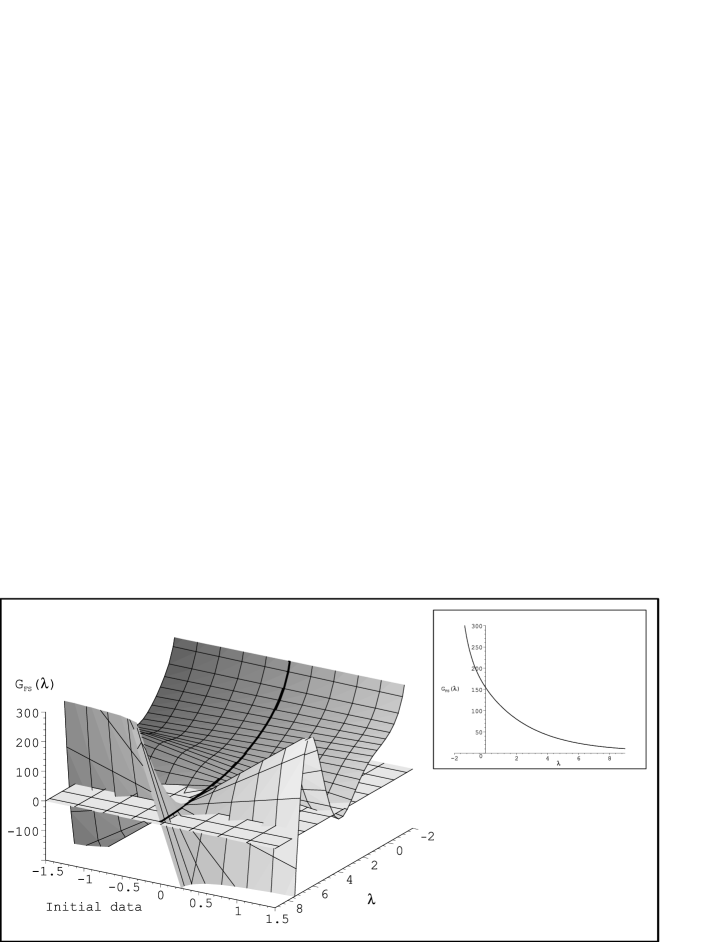
Figure 1: Gauge orbits in boson string field theory.

$$a =1.13\,t_{0}-2.13\,v_{0}+0.997\,u_{0}+0.921\,w_{0}-0.0861,$$ (5.14a)

$$b =0.172\,t_{0}-0.939\,v_{0}-0.346\,u_{0}+1.04\,w_{0}-1.49,$$ (5.14b)

$$c =0.0466\,t_{0}+0.300\,v_{0}-0.0149\,u_{0}-0.00958\,w_{0}-0.741,$$ (5.14c)

$$d =-0.218\,t_{0}+0.639\,v_{0}+0.360\,u_{0}-0.0337\,w_{0}-0.657.$$ (5.14d)

If one takes an initial point $\{t_{0},\,v_{0},\,u_{0},\,w_{0}\}$ such that $a=b=0$ and $c,d\geqslant 0$ then the corresponding gauge orbit never intersects the surface $G_{FS}(\phi^{i})=0$ This situation is depicted in Figure 1 by the thick line on 3-dimensional plot and by 2-dimensional plot.

5.2 Orbits in Superstring Field Theory

Performing similar calculations in cubic SSFT we get the following results. The characteristic polynomial $\mathscr{P}$ of the matrix $\mathscr{J}^{i}{}_{j}$ is

$$\mathscr{P}(\mathscr{J},\omega)=\bigl{(}\omega^{4}-\frac{1187840}{59049}\omega^{2}+\frac{451911090176}{3486784401}\bigr{)}\bigl{(}\omega+\frac{256}{729}\sqrt{3}\bigr{)}\omega^{4}$$ (5.15)

The eigenvalues of the matrix $\mathscr{J}^{j}{}_{i}$ are

$$\{\omega\}=\{0,\,0,\,0,\,0,\,-0.608,\,\eta\}\qquad\text{where}\qquad\eta=\pm 3.274\pm i0.814$$ (5.16)

with the corresponding eigenvectors

$$\nu_{0}^{(1)}=\begin{bmatrix}1\\ 0\\ 0\\ -5.4\\ 0\\ 0\\ 0\\ 0\\ 0\end{bmatrix},\qquad\nu_{0}^{(2)}=\begin{bmatrix}0\\ 0\\ 0\\ 39.3\\ 1\\ 2\\ 0\\ -6\\ -2\end{bmatrix},\qquad\nu_{0}^{(3)}=\begin{bmatrix}0\\ 0\\ 1\\ 7.5\\ 0\\ 0\\ 0\\ 0\\ 0\end{bmatrix},\qquad\nu_{0}^{(4)}=\begin{bmatrix}0\\ 1\\ 0\\ 155.6\\ 0\\ 0\\ 0\\ -18\\ -8\end{bmatrix},$$ (5.17)

$$\nu_{-0.608}=\begin{bmatrix}0\\ 0\\ 0\\ 0\\ 0\\ 0\\ 1\\ 0\\ 0\end{bmatrix},\qquad\nu_{\eta}=\begin{bmatrix}0.011\eta^{3}-0.17\eta^{2}+0.12\eta-1.77\\ -0.015\eta^{3}+0.022\eta^{2}-0.16\eta-0.28\\ 0.5\\ 1\\ 0.038\eta^{3}+0.26\eta^{2}+0.39\eta-0.044\\ -0.03\eta^{3}+0.044\eta^{2}+\eta+1.95\\ 0\\ 0.29\eta^{3}+0.995\eta^{2}-2.27\eta-7.33\\ 0.12\eta^{3}+0.54\eta^{2}-0.13\eta-2.97\end{bmatrix}.$$ (5.18)

The solution of (5.2) yields the gauge orbits of gauge fixing function (5.1)

$$G(\phi)=[a\sin(0.814\lambda)+b\cos(0.814\lambda)]e^{3.27\lambda}\\ +[c\sin(0.814\lambda)+d\cos(0.814\lambda)]e^{-3.27\lambda}+4.15\lambda+f,$$ (5.19)

where

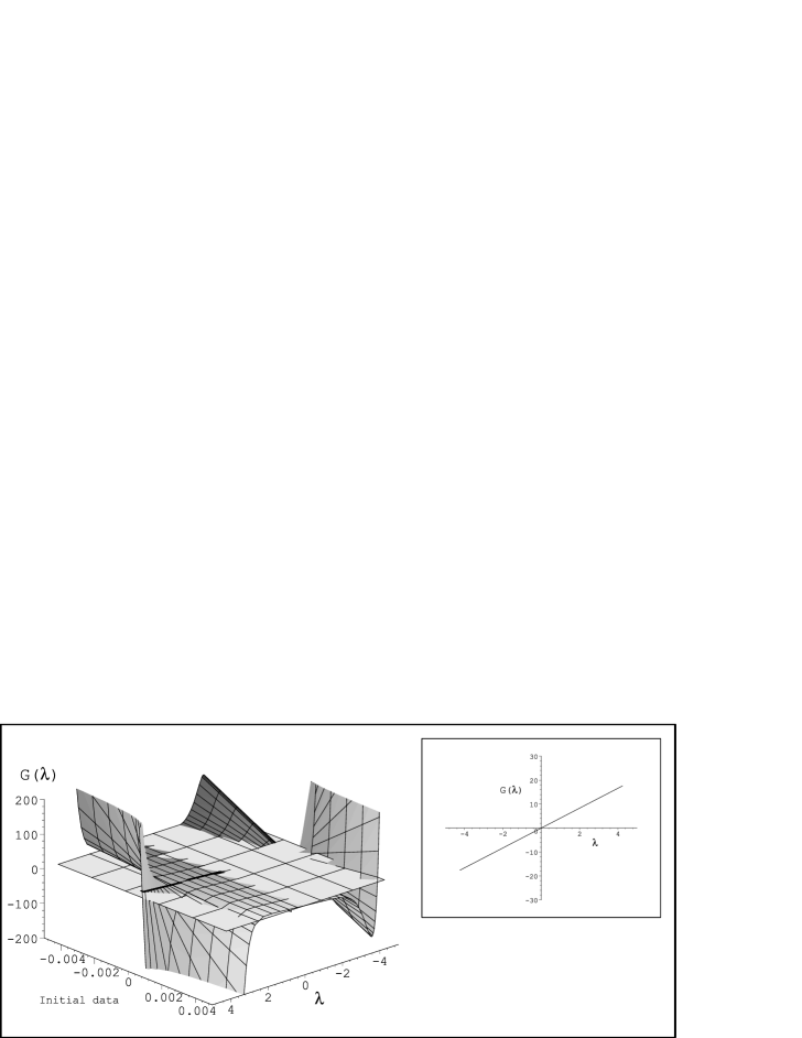
Figure 2: Gauge orbits in NS string field theory.

$$a =-1.05u_{0}-2.81v_{1,0}+1.46v_{2,0}-0.195v_{3,0}$$

$$~{}~{}~{}~{}~{}~{}~{}~{}~{}~{}+5.82v_{4,0}-4.81v_{5,0}-2.13v_{7,0}+0.614v_{8,0}-0.177$$ (5.20a)

$$b =-0.406u_{0}-1.04v_{1,0}+0.559v_{2,0}-0.0754v_{3,0}$$

$$~{}~{}~{}~{}~{}~{}~{}~{}~{}~{}-0.03v_{4,0}-0.59v_{5,0}-0.64v_{7,0}-0.155v_{8,0}-0.924$$ (5.20b)

$$c =-0.0933u_{0}-1.38v_{1,0}+0.130v_{2,0}-0.0174v_{3,0}$$

$$~{}~{}~{}~{}~{}~{}~{}~{}~{}~{}+1.06v_{4,0}-0.572v_{5,0}+0.166v_{7,0}-0.885v_{8,0}+0.516$$ (5.20c)

$$d =-0.0636u_{0}+0.104v_{1,0}+0.088v_{2,0}-0.0118v_{3,0}$$

$$~{}~{}~{}~{}~{}~{}~{}~{}~{}~{}+0.552v_{4,0}-0.195v_{5,0}+0.085v_{7,0}-0.407v_{8,0}-0.186$$ (5.20d)

$$f =0.465u_{0}+0.939v_{1,0}+2.35v_{2,0}+0.0867v_{3,0}$$

$$~{}~{}~{}~{}~{}~{}~{}~{}~{}~{}-3.51v_{4,0}+2.77v_{5,0}+0.56v_{7,0}+0.563v_{8,0}+1.12$$ (5.20e)

and $u_{0},v_{i,0}$ are initial data for the corresponding differential equations (5.2).

A simple analysis shows that there are no restrictions on the range of validity of the gauge (5.1) (see Figure 2). The 2-dimensional plot on the Figure 2 corresponds to the special initial data $a=b=c=d=0$.

It is interesting to note that there is another gauge which strongly simplifies the effective potential. Namely, this is the gauge $v_{6}=0$. The orbits of this gauge condition have the form

$$v_{6}(\lambda)=(1.64+v_{6,0})e^{-0.608\lambda}-1.64$$

It is evident that this gauge condition is not always reachable and cannot be used in the calculation of the tachyon potential.

6 Summary

We have presented the restricted cubic superstring action (2.2) that contains fields only from $V_{0}$ and $V_{1}$ spaces. One can consider this superselection rule as a partial gauge fixing. Then we have described a method of calculation of $\star$-product without using the direct expression through Neumann functions. Using this method we have computed the gauge transformations of the action truncated to level $(2,6)$. In contrast to bosonic string field theory the gauge invariance in level truncation scheme is broken not only in the second order in coupling constant, but already in the first order. We have made an estimation of this breaking using an example of $t^{2}$-terms in gauge variation of the truncated action. It is shown that this breaking originated from the contributions of higher level fields is about $33\%$. This gives us a hope that the gauge invariance rapidly restores as level grows.

We have explored a validity of our gauge condition (5.1) in cubic SSFT as well as Feynman-Siegel one in boson SFT. We have shown that every gauge orbit in cubic SSFT necessarily intersects our gauge fixing surface (5.1) at least once (see Figure 2). Hence our gauge is valid for computation of extremum of the action. For Feynman-Siegel gauge in the bosonic SFT we have shown that there are field configurations with orbits which never intersect the gauge fixing surface (see Figure 1).

Appendix

Appendix A Notations

Here we collect notations that we use in our calculations (for more details see [18]).

Table 2: Notations and OPE-s.

$X_{L}^{\mu}(z)X_{L}^{\nu}(w)\sim-\frac{\alpha^{\prime}}{2}\eta^{\mu\nu}\log(z-w)$	$\psi^{\mu}(z)\psi^{\nu}(w)\sim-\frac{\alpha^{\prime}}{2}\eta^{\mu\nu}\frac{1}{z-w}$
$c(z)b(w)\sim b(z)c(w)\sim\frac{1}{z-w}$	$\gamma(z)\beta(w)\sim-\beta(z)\gamma(w)\sim\frac{1}{z-w}$
$\gamma=\eta e^{\phi}$	$\beta=e^{-\phi}\partial\xi$
$\phi(z)\phi(w)\sim-\log(z-w)$	$\xi(z)\eta(w)\sim\eta(z)\xi(w)\sim\frac{1}{z-w}$
$T_{B}=-\frac{1}{\alpha^{\,\prime}}\partial X\cdot\partial X-\frac{1}{\alpha^{\,\prime}}\partial\psi\cdot\psi$	$T_{F}=-\frac{1}{\alpha^{\,\prime}}\partial X\cdot\psi$
$T_{bc}=-2b\partial c-\partial bc$	$T_{\beta\gamma}=-\frac{3}{2}\beta\partial\gamma-\frac{1}{2}\partial\beta\gamma$
$T_{\phi}=-\frac{1}{2}\partial\phi\partial\phi-\partial^{2}\phi$	$T_{\eta\xi}=\partial\xi\eta$
$Q_{B}=Q_{0}+Q_{1}+Q_{2}$
$Q_{0}=\frac{1}{2\pi i}\oint d\zeta\,\left[c(T_{B}+T_{\phi}+T_{\eta\xi})+bc\partial c\right]$
$Q_{1}=\frac{1}{2\pi i}\oint d\zeta\,\left[\frac{1}{\alpha^{\,\prime}}\eta e^{\phi}\psi\cdot\partial X\right]$
$Q_{2}=\frac{1}{2\pi i}\oint d\zeta\,\left[\frac{1}{4}b\partial\eta\eta e^{2\phi}\right]$
$Y=4c\partial\xi e^{-2\phi}$

Appendix B Conformal Transformations of the Dual Fields

Taylor series of maps (2.4) in the origin:

$$F_{1}(w) =1+2\gamma w+3\gamma^{2}w^{2}+\frac{31}{8}\gamma^{3}w^{3}+\frac{39}{8}\gamma^{4}w^{4}+\frac{813}{128}\gamma^{5}w^{5}+\dots$$ (B.1a)

$$F_{2}(w) =\frac{1}{2}\gamma w-\frac{5}{32}\gamma^{3}w^{3}+\frac{57}{512}\gamma^{5}w^{5}+\dots$$ (B.1b)

$$F_{3}(w) =-1+2\gamma w-3\gamma^{2}w^{2}+\frac{31}{8}\gamma^{3}w^{3}-\frac{39}{8}\gamma^{4}w^{4}+\frac{813}{128}\gamma^{5}w^{5}+\dots$$ (B.1c)

Here $\gamma=\frac{4}{3\sqrt{3}}$.

Below we present conformal transformations, necessary to map dual vertex operators (3.10)

$$(f\circ\eta)(w) ={f^{\prime}}\eta(f)$$

$$(f\circ\partial\eta)(w) ={f^{\prime}}^{2}\partial\eta(f)+{f^{\prime\prime}}\eta(f)$$

$$(f\circ\partial^{2}\eta)(w) ={f^{\prime\prime\prime}}\eta(f)+3{f^{\prime}}{f^{\prime\prime}}\partial\eta(f)+{f^{\prime}}^{3}\partial^{2}\eta(f)$$

$$(f\circ T_{B})(w) ={f^{\prime}}^{2}T_{B}(f)+\frac{15}{12}\left(\frac{{f^{\prime\prime\prime}}}{{f^{\prime}}}-\frac{3}{2}\frac{{f^{\prime\prime}}^{2}}{{f^{\prime}}^{2}}\right)$$

$$(f\circ T_{F})(w) ={f^{\prime}}^{3/2}T_{F}(f)$$

$$(f\circ\partial(bc))(w) ={f^{\prime}}^{2}\partial(bc)(f)+{f^{\prime\prime}}b(f)c(f)+\frac{3}{2}\left(\frac{{f^{\prime\prime\prime}}}{{f^{\prime}}}-\frac{{f^{\prime\prime}}^{2}}{{f^{\prime}}^{2}}\right)$$

$$(f\circ\partial bc)(w) ={f^{\prime}}^{2}\partial b(f)c(f)+2{f^{\prime\prime}}b(f)c(f)+\frac{5}{6}\frac{{f^{\prime\prime\prime}}}{{f^{\prime}}}+\frac{1}{4}\frac{{f^{\prime\prime}}^{2}}{{f^{\prime}}^{2}}$$

$$(f\circ b\partial c)(w) ={f^{\prime}}^{2}b(f)\partial c(f)-{f^{\prime\prime}}b(f)c(f)+\frac{2}{3}\frac{{f^{\prime\prime\prime}}}{{f^{\prime}}}-\frac{7}{4}\frac{{f^{\prime\prime}}^{2}}{{f^{\prime}}^{2}}$$

$$(f\circ e^{q\phi})(w) ={f^{\prime}}^{-\tfrac{1}{2}q(q+2)}e^{q\phi(f)}$$

$$(f\circ\partial\phi e^{2\phi})(w) =\frac{1}{{f^{\prime}}^{3}}\partial\phi(f)e^{2\phi(f)}-2\frac{{f^{\prime\prime}}}{{f^{\prime}}^{5}}e^{2\phi(f)}$$

$$(f\circ(\partial\phi)^{2}e^{2\phi})(w) =\frac{1}{{f^{\prime}}^{2}}\partial\phi(f)\partial\phi(f)e^{2\phi(f)}-4\frac{{f^{\prime\prime}}}{{f^{\prime}}^{4}}\partial\phi(f)e^{2\phi(f)}+\frac{1}{{f^{\prime}}^{4}}\left(-\frac{1}{6}\frac{{f^{\prime\prime\prime}}}{{f^{\prime}}}+\frac{17}{4}\frac{{f^{\prime\prime}}^{2}}{{f^{\prime}}^{2}}\right)e^{2\phi(f)}$$

$$(f\circ\partial^{2}\phi e^{2\phi})(w) =\frac{1}{{f^{\prime}}^{2}}\partial^{2}\phi(f)e^{2\phi(f)}+\frac{{f^{\prime\prime}}}{{f^{\prime}}^{4}}\partial\phi(f)e^{2\phi(f)}+\frac{1}{{f^{\prime}}^{4}}\left(\frac{3}{2}\frac{{f^{\prime\prime}}^{2}}{{f^{\prime}}^{2}}-\frac{5}{3}\frac{{f^{\prime\prime\prime}}}{{f^{\prime}}}\right)e^{2\phi(f)}$$

References

• [1] A. Sen, Stable non BPS bound states of bps d-branes, JHEP 08, 010 (1998), hep-th/9805019;
A. Sen, SO(32) spinors of type I and other solitons on brane - anti-brane pair, JHEP 09, 023 (1998), hep-th/9808141;
A. Sen, Universality of the Tachyon Potential JHEP 9912 (1999) 027, hep-th/9911116
• [2] A. Sen, B. Zwiebach, Tachyon condensation in string field theory, JHEP 0003 (2000) 002, hep-th/9912249;
N.Moeller, W.Taylor, Level truncation and the tachyon in open bosonic string field theory, Nucl.Phys. B583 (2000) 105-144, hep-th/0002237;
P. De Smet, J. Raeymaekers, Level Four Approximation to the Tachyon Potential in Superstring Field Theory, JHEP 0005 (2000) 051, hep-th/0003220;
P.-J. De Smet, J. Raeymaekers The Tachyon Potential in Witten’s Superstring Field Theory, JHEP 0008 (2000) 020, hep-th/0004112;
W. Taylor, Mass generation from tachyon condensation for vector fields on D-branes JHEP 0008 (2000) 038, hep-th/0008033;
A. Minahan, Barton Zwiebach, Field theory models for tachyon and gauge field string dynamics, JHEP 0009 (2000) 029hep-th/0008231;
A.Kostelecky and R. Potting, Analytical construction of a nonperturbative vacuum for the open bosonic string, hep-th/0008252;
H. Hata, Sh. Shinohara, BRST Invariance of the Non-Perturbative Vacuum in Bosonic Open String Field Theory JHEP 0009 (2000) 035, hep-th/0009105;
D. Ghoshal and A. Sen, Normalisation of the background independent open string field theory action, JHEP 0011, 021 (2000) hep-th/0009191;
B. Zwiebach, Trimming the tachyon string field with SU(1,1), hep-th/0010190;
Ashoke Sen, Fundamental Strings in Open String Theory at the Tachyonic Vacuum, hep-th/0010240;
L.Rastelli, A.Sen, B.Zwiebach, String field theory around the tachyon vacuum, hep-th/0012251;
P. Mukhopadhyay and A. Sen, Test of Siegel gauge for the lump solution, JHEP 0102, 017 (2001), hep-th/0101014;
H. Hata, Sh. Teraguchi, Test of the Absence of Kinetic Terms around the Tachyon Vacuum in Cubic String Field Theory, JHEP 0105 (2001) 045, hep-th/0101162;
K. Ohmori, A Review on Tachyon Condensation in Open String Field Theories, hep-th/0102085;
Leonardo Rastelli, Ashoke Sen, Barton Zwiebach, Classical Solutions in String Field Theory Around the Tachyon Vacuum hep-th/0102112;
I. Ellwood, W. Taylor, Open string field theory without open strings, hep-th/0103085;
D.J. Gross and W. Taylor, Split string field theory I,II, hep-th/0105059,hep-th/0106036;
D.J. Gross and W. Taylor, String field theory, non-commutative Chern-Simons theory and Lie algebra cohomolog, hep-th/0106242;
K.Ohmori, Survey of the tachyonic lump in bosonic string field theory, hep-th/0106068.
• [3] N. Berkovits, A. Sen, B. Zwiebach, Tachyon Condensation in Superstring Field Theory, hep-th/0002211;
J. Kluson, Proposal for background independent Berkovits superstring field theory, hep-th/0106107.
• [4] E. Witten, On background-independent open-string field theory, Phys. Rev. D46, 5467 (1992);
A. A. Gerasimov, S. L. Shatashvili, Stringy Higgs Mechanism and the Fate of Open Strings, hep-th/0011009;
D. Kutasov, M. Mariño and G. Moore, Remarks on Tachyon Condensation in Superstring Field Theory, hep-th/0010108;
P. Kraus and F. Larsen, Boundary String Field Theory of the $D\bar{D}$ System, hep-th/0012198;
S.P. de Alwis, Boundary String Field Theory, the Boundary State Formalism and D-Brane Tension, hep-th/0101200;
V. Niarchos, N. Prezas, Boundary Superstring Field Theory, hep-th/0103102;
M. Marino, On the BV formulation of boundary superstring field theory, JHEP 0106:059,2001; hep-th/0103089;
K. S. Viswanathan and Y. Yang, Tachyon Condensation and Background Indepedent Superstring Field Theory, hep-th/0104099;
M. Alishahiha, One-loop Correction of the Tachyon Action in Boundary Superstring Field Theory, hep-th/0104164;
K. Bardakci and A. Konechny, Tachyon condensation in boundary string field theory, hep-th/0105098;
T. Lee, Tachyon Condensation, Boundary State and Noncommutative Solitons, hep-th/0105115;
G. Arutyunov, A. Pankiewicz and B. Stefa nski, jr., Boundary Superstring Field Theory Annulus Partition Function in the Presence of Tachyons, hep-th/0105238;
S. Viswanathan, Y. Yang, Unorientable Boundary Superstring Field theory with Tachyon field, hep-th/0107098.
• [5] I.Ya. Aref’eva, D.M. Belov, A.S. Koshelev and P.B. Medvedev, Tachyon Condensation in the Cubic Superstring Field Theory, hep-th/0011117
• [6] I.A. Aref’eva, P.B. Medvedev and A.P. Zubarev, Background formalism for superstring field theory, Phys.Lett. B240, pp.356–362 (1990)
• [7] C.R. Preitschopf, C.B. Thorn and S.A. Yost, Superstring Field Theory, Nucl.Phys.B337(1990)363.
• [8] I.Ya.Aref’eva, P.B.Medvedev and A.P.Zubarev, New representation for string field solves the consistency problem for open superstring field, Nucl.Phys. B341, pp.464–498 (1990)
• [9] C.B. Thorn, String field theory, Phys.Rept.,175(1989)1.
• [10] V.A.Kostelecky and S.Samuel, The static tachyon potential in the open bosonic string theory, Phys.Lett.  B207 (1988), p.659;
V.A.Kostelecky and S.Samuel, The tachyon potential in string sheory, DPF Conf. pp.813–816 (1989);
V.A.Kostelecky and S.Samuel, On a nonperturbative vacuum for the open bosonic string, Nucl.Phys. (1989) B336, p.28
• [11] I. Ellwood, W. Taylor, Gauge Invariance and Tachyon Condensation in Open String Field Theory, hep-th/0105156
• [12] A. LeClair, M. Peskin and C. Preitschopf, String Field Theory on the Conformal Plane, I, Nucl. Phys. B317 (1989) 411-463.
• [13] E. Witten, Noncommutative geometry and string field theory, Nucl. Phys. B268 (1986), 253.
E. Witten, Noncommutative Geometry and String Field Theory, Nucl. Phys. B207 (1488), p.169
• [14] D. Gross and A. Jevicki, Operator Formulation of Interacting String Field Theory, (I), (II), Nucl.Phys. B283 (1987) 1; Nucl.Phys B287 (1987) 225.
• [15] I.Ya. Aref’eva, D.M. Belov, A.S. Koshelev and P.B. Medvedev, Lecture notes on Cubic Superstring Field Theory, work in progress
• [16] I.Ya. Aref’eva, P.B. Medvedev, Truncation, picture changing operation and space time supersymmetry in Neveu- Schwarz-Ramond string field theory. Phys.Lett.B202 (1988) 510.
• [17] L. Rastelli and B. Zwiebach, Tachyon potentials, star products and universality, hep-th/0006240.
• [18] D. Friedan, E. Martinec, and S. Shenker, Conformal Invariance, Supersymmetry, and String Theory, Nucl. Phys.B 271 (1986) 93.