Non-abelian plane waves and stochastic regimes for (2+1)-dimensional gauge field models with Chern-Simons term

Abstract

An exact time-dependent solution of field equations for the 3-d gauge field model with a Chern-Simons (CS) topological mass is found. Limiting cases of constant solution and solution with vanishing topological mass are considered. After Lorentz boost, the found solution describes a massive nonlinear non-abelian plane wave. For the more complicate case of gauge fields with CS mass interacting with a Higgs field, the stochastic character of motion is demonstrated.

I Introduction

The non-abelian Yang-Mills (YM) gauge field theory is essentially nonlinear. In particular, such characteristic infrared phenomena of QCD as confinement and chiral symmetry breaking are explained by the nonlinear nature of gluon interactions leading to the formation of specific nonperturbative configurations of gauge fields responsible for these phenomena. Various exact topologically nontrivial finite energy solutions of the classical gauge field equations in (3+1)-dimensional space-time with or without Higgs fields (e.g. instantons[1], vortices [2], monopoles [3]) as well as non-abelian plane-wave solutions [4], [5], [6], [7] have been found (for a detailed discussion of YM equations, see, e.g., [10],[11]). In (2+1)-dimensional space-time, a nonlinear topological term (the so called Chern-Simons (CS) secondary character) which is responsible for formation of a topological mass of the non-abelian gauge field, may be added to the field Lagrangian [8]. In this case, constant non-abelian solutions of the gauge field equations with a CS mass were found [9]. Clearly, the investigation of general properties of classical solutions of gauge field equations is important and may provide new knowledge about the vacuum structure of a given theory. Among these properties the irregular stochastic character of the gauge field dynamics is of great interest (see [12]). The stochastic behavior of the YM theory has been studied in the pioneering papers [5], [6], [13], [14], [15]. The consideration of possible interactions with a Higgs field is also interesting, but makes the problem somewhat more complicated. Investigations of the stochastic behavior of classical field systems with Higgs fields but without Chern-Simons term were e.g. made in [7]. Moreover, numerical investigations of Poincare sections of the YM-Higgs theory with an $SU(2)$ doublet Higgs field were performed in [14]. Taking only the vacuum expectation value of the Higgs field into account, the authors of this paper showed qualitatively the stabilizing role of the Higgs mechanism for the YM dynamics. Furthermore, in [18] the dynamical contribution of Higgs fields was considered. It was shown that a field system with spatially uniform but time-dependent dynamical Higgs fields, coupled to a gauge field ($SO(3)$ Georgi-Glashow model), also demonstrates chaotic behavior with certain threshold values of the energy.

It is further worth noticing that the chaotic dynamics of the three-dimensional topologically massive gauge fields (without Higgs fields) was also studied in the framework of the time-dependent and spatially-uniform Chern-Simons model in ref. [21]. The numerical studies of the CS field equations were performed there by the Runge-Kutta method. The boundary conditions were chosen in such a way that all three gauge potentials, now being considered as coordinates of fictitious “particles”, were put on a circle. The general motion might thus be interpreted as that of three effective particles moving in a plane and interacting nonlinearly through a quartic potential and under the influence of an “external magnetic field” of strength $\mu$ ($\mu$ is a topological mass). It was demonstrated that a background “magnetic field” tries to order the system, forcing the “particles” to move in periodic orbits, similar to the influence of a Higgs condensate on the otherwise chaotic classical YM dynamics. Therefore, if the strength $\mu$ of the topological term is large compared to the energy density (in the quantized theory, this would mean strong coupling), the motion is regular, while in the opposite case it is chaotic. This “order to chaos transition” was observed in numerical studies of the CS-model as well as in the coupled YM-Higgs model, although the two models differ in many respects. Note also that the transition from regularity to irregularity in quantum systems, which are classically chaotic, was considered for a $d=(2+1)$ YM-Higgs theory in [19].

In the present paper, we consider the generalization of the plane-wave solutions, found earlier in the $d=3+1$-case (see[4], [5], [6], [7]), to the case of a (2+1)-dimensional gauge field theory with topological Chern-Simons term. Clearly, the topological mass provides an additional dimensional parameter for the massive nonlinear field configuration in question. In this way, we find a new plane-wave solution of the corresponding field equations. Next, the possibility of passing to a constant background field [9] with energy density lower than the perturbative vacuum energy is considered. Moreover, we demonstrate that the dynamics of 3-d YM fields with a CS topological mass interacting with Higgs fields is described by solutions that, generally speaking, are not regular, but rather obtain ergodic properties. This study was made for an ansatz which is specific for the gauge fields in (2+1)-dimensional space-time and different from that considered earlier in the (3+1)-d case without CS term or in the (2+1)-d case with CS term. Our numerical study of the stochastic properties of solutions with growing energy demonstrates that a chaotic behavior of solutions is observed mostly for those values of the energy which are near to the critical “saddle” point value of the potential energy of the effective mechanical system. We emphasize that we have also considered the important case of spontaneous symmetry breaking in the CS-Georgi-Glashow model (where the mass term has the sign required for spontaneous symmetry breaking, and the real mass squared is negative $-m^{2}<0$). Finally, the dynamics of a system of coupled gauge and Higgs fields is investigated in the general case, where fairly large values of the energy are admitted and, in contrast to earlier work, no assumptions are made that the system is near a stable solution (near the “minimum” critical point of the effective potential).

II Time-dependent solutions

Consider a 3-dimensional $SU(2)$ gauge field theory with a Chern-Simons term. The gauge field Lagrangian can be written as follows

$${\cal L}_{g}=-\frac{1}{4}F_{\mu\nu}^{a}F^{\mu\nu{a}}+\frac{\mu}{4}\epsilon^{\mu\nu\alpha}[F_{\mu\nu}^{a}A_{\alpha}^{a}-\frac{g}{3}\epsilon^{abc}A_{\mu}^{a}A_{\nu}^{b}A_{\alpha}^{c}],$$ (1)

where $F_{\mu\nu}^{a}=\partial_{\mu}A_{\nu}^{a}-\partial_{\nu}A_{\mu}^{a}+g\epsilon^{abc}A_{\mu}^{b}A_{\nu}^{c}$ is the gauge field tensor. The last term in (1) is the CS term [8] that describes the topological mass $\mu$ of the gauge field.

The Lagrangian (1) is not gauge invariant, since it changes by a full derivative under a gauge transformation

$$S=\int d^{3}x{\cal L}_{g}\longrightarrow\int d^{3}x{\cal L}_{g}+\mu(8\pi^{2}/g^{2})W(U),$$ (2)

where

$$W(U)=\frac{1}{24\pi^{2}}\int d^{3}x\epsilon^{\alpha\beta\gamma}\mathop{\rm tr}\nolimits[\partial_{\alpha}UU^{-1}\partial_{\beta}UU^{-1}\partial_{\gamma}UU^{-1}],$$ (3)

and $U(x)=\exp[i\sigma^{a}\theta^{a}(x)]$. Here $W(U)$ is the “winding number” of the gauge transformation $U(x)$, $\sigma^{a}$ are Pauli matrices. In order to make $\exp(iS)$ gauge-invariant, the Chern-Simons parameter $\mu$ should be quantized [8]

$$\mu=\frac{g^{2}n}{4\pi},n\in Z.$$ (4)

From the Lagrange equations

$$\frac{\partial{\cal L}_{g}}{\partial A_{\nu}^{a}}-\frac{\partial}{\partial x^{\mu}}\frac{\partial{\cal L}_{g}}{\partial A_{\nu,\mu}^{a}}=0,$$ (5)

one obtains the field equation

$$D_{\nu}F^{\nu\mu a}+\frac{\mu}{2}\epsilon^{\mu\alpha\beta}F_{\alpha\beta}^{a}=0,$$ (6)

where $D_{\mu}F_{\alpha\beta}^{a}=\partial_{\mu}F_{\alpha\beta}^{a}+g\epsilon^{abc}A_{\mu}^{b}F_{\alpha\beta}^{c}$ .

Let us seek solutions $A_{\mu}^{a}=A_{\mu}^{a}(t)$ that depend only on the time $t$, but not on coordinates $\bf x$ and choose the following rather restrictive ansatz

$$A_{\mu}^{a}=\delta_{\mu}^{a}f_{a}(t),\ A^{\mu a}=g^{\mu a}f_{a}(t),$$ (7)

$$a=1,2,3,\ \mu=1,2,3\ (x_{1}=t,x_{2}=x,x_{3}=y),$$ (8)

$$g_{\mu\nu}={\mbox{diag}}(+,-,-),$$ (9)

where no summation over $a$ is assumed. This case formally corresponds to a mechanical system with a finite number of degrees of freedom, whose motion is described by the system of equations

$$\mu gf_{2}f_{3}+g^{2}f_{1}(f_{2}^{2}+f_{3}^{2})=0,$$ (11)

$$\mu gf_{1}f_{3}-\ddot{f_{2}}+g^{2}f_{2}(f_{1}^{2}-f_{3}^{2})=0,$$ (12)

$$\mu gf_{1}f_{2}-\ddot{f_{3}}+g^{2}f_{3}(f_{1}^{2}-f_{2}^{2})=0,$$ (13)

$$\mu\dot{f_{2}}+g(\dot{f_{1}}f_{3}+2f_{1}\dot{f_{3}})=0,$$ (14)

$$\mu\dot{f_{3}}+g(\dot{f_{1}}f_{2}+2f_{1}\dot{f_{2}})=0,$$ (15)

where $\dot{f_{a}}=\frac{\partial f_{a}}{\partial t}$ . It is evident that these equations describe three coupled unharmonical oscillators. It is interesting to note that for $f_{1}=f_{2}=f_{3}=f$ only a trivial solution exists, i.e., $f=0$. Thus, in order to find a non-trivial solution, the functions $f_{a}$ should not be taken equal. Let us seek solutions from the class $f_{1}\neq f_{2}=f_{3}=f$. In this case, one obtains

$$\mu gf^{2}+2g^{2}f_{1}f^{2}=0,$$ (16)

$$\mu gf_{1}f-\ddot{f}+g^{2}f(f_{1}^{2}-f^{2})=0,$$ (17)

$$\mu\dot{f}+g(\dot{f_{1}}f+2f_{1}\dot{f})=0.$$ (18)

First of all, we mention that this system of equations has constant solutions, found earlier in [9]

$$f_{1}=-\frac{\mu}{2g},\ f_{2}=f_{3}=\pm i\frac{\mu}{2g}.$$ (19)

Solutions that depend on time can also be found

$$f_{1}=-\frac{\mu}{2g},$$ (20)

$$f_{2}=f_{3}=f(t).$$ (21)

Then the corresponding chromoelectric and chromomagnetic field components are defined as follows

$$E^{a}_{i}=F^{a}_{1i},$$ (22)

$$E^{1}_{i}=(0,0,0),\ E^{2}_{i}=(0,\dot{f},\frac{\mu}{2}f),\ E^{3}_{i}=(0,-\frac{\mu}{2}f,\dot{f})$$ (23)

$$H^{a}=\frac{1}{2}\epsilon^{ij}F^{a}_{ij},\ H^{1}=gf^{2},\ H^{2}=H^{3}=0.$$ (24)

The function $f(t)$ satisfies the following nonlinear differential equation

$$\ddot{f}+\frac{\mu^{2}}{4}f+g^{2}f^{3}=0.$$ (25)

This equation has a first integral which is the energy integral of motion $\cal E$ for our mechanical system

$$\dot{f}^{2}+\frac{g^{2}}{2}f^{4}+\frac{\mu^{2}}{4}f^{2}=const={\cal E}.$$ (26)

At the same time ${\cal E}$ is the energy density of the Yang-Mills field corresponding to the $T^{0}_{0}$ component of the energy-momentum tensor of the field

$$T^{0}_{0}={\cal E}=\frac{1}{2}((H^{a})^{2}+(E_{i}^{a})^{2}).$$

Note that the Chern-Simons term gives no contribution to the energy density.

The equation (26) can be easily integrated

$$\int\frac{df}{\sqrt{{\cal E}-\frac{g^{2}}{2}f^{4}-\frac{\mu^{2}}{4}f^{2}}}=t-t_{0}.$$ (27)

This integral can be expressed in terms of the elliptic functions,

$$f(t)=\frac{\mu}{\sqrt{2}g}\frac{k}{\sqrt{1-2k^{2}}}\mathop{\rm cn}\nolimits\left((\frac{\mu^{4}}{16}+2{\cal E}g^{2})^{\frac{1}{4}}(t-t_{0}),k\right),$$ (28)

where $\mathop{\rm cn}\nolimits(x,k)$ is the elliptic Jacobi cosine function of the argument $x$ and the module $k$ [22]

$$k=\sqrt{\frac{1}{2}\bigg{(}1-\frac{\mu^{2}}{4(\frac{\mu^{4}}{16}+2{\cal E}g^{2})^{\frac{1}{2}}}\bigg{)}}.$$ (29)

This solution is periodical with the period

$$T=\frac{4{\rm K}(k)}{({\frac{\mu^{4}}{16}+2{\cal E}g^{2}})^{\frac{1}{4}}},$$ (30)

where ${\rm K}(x)$ is a full elliptic integral of the first kind [22].

The oscillation period is inversely proportional to the combination of the dimensional parameters of the theory, i.e. the CS mass $\mu$ and the energy of the solution $\cal E$. This, evidently, could be predicted without solving the equation: there are two scales in the equations, one of them is provided by a characteristic amplitude of the field $gA\sim({\cal E}g^{2})^{1/4}$, whose dimension is $[(gA)]=m\sim 1/T$, and the other is the Chern-Simons parameter with the dimension of a mass $[\mu]=m$.

Since the solution is a function of time only and does not depend on spatial coordinates, this corresponds to the rest frame of reference for the field configuration. Therefore, it is quite natural that $P^{i}=T^{0i}=0$, i.e., the energy flux is equal to zero in this frame.

Note that the constant solution (19) can be obtained from the solution (28) in the limit of an infinite period $T\rightarrow\infty$. This is achieved, if we allow ${\cal E}$ to be equal to $-\frac{\mu^{4}}{32g^{2}}$

$${\cal E}\rightarrow-\frac{\mu^{4}}{32g^{2}},\ T\rightarrow\infty,\ \frac{k}{\sqrt{1-2k^{2}}}\rightarrow\pm\frac{i\mu}{\sqrt{2}}$$ (31)

$$f(t)\rightarrow\ \pm\frac{i\mu}{2g}.$$ (32)

It is evident that this limiting procedure can be performed only if complex values of $f$ are allowed. In this case, the energy ${\cal E}$ remains real, though it becomes negative, which indicates a possibility of lowering the gauge field energy.

Using our solution, we can pass to the limit of a vanishing Chern-Simons term corresponding to the Lagrangian

$${\cal L}_{g}=-\frac{1}{4}F_{\mu\nu}^{a}F^{\mu\nu{a}}.$$

To this end, we assume $\mu\rightarrow 0,A_{1}^{1}\rightarrow 0$ . As a result, the following limiting solution is received

$$A_{1}^{1}=0,A_{2}^{2}=A_{3}^{3}=(\frac{2{\cal E}}{g^{2}})^{\frac{1}{4}}\mathop{\rm cn}\nolimits\Big{(}\ (2{\cal E}g^{2})^{\frac{1}{4}}(t-t_{0}),1/\sqrt{2}\Big{)}.$$ (33)

It should be mentioned that a similar solution was obtained in ref.[5, 6] for the case of a 4-dimensional Yang-Mills theory without Chern-Simons term.

III Plane-wave solutions

The solution (28) describes a nonlinear standing wave. By applying a Lorentz boost, one can obtain nonlinear propagating waves.  It is easy to see that the argument of the above periodical solution can be Lorentz transformed in the following way: $x^{\prime}_{\mu}=a_{\mu}^{\nu}(\vec{v})x_{\nu}$, $kx=k^{\prime}x^{\prime}$, where:

$$k^{\prime}_{0}=M\gamma,k^{\prime}_{i}=Mv_{i}\gamma,(\gamma=(1-v^{2})^{-1/2}).$$ (34)

Here $M$ has the meaning of a mass, since $k^{2}=M^{2}$.

As was already mentioned above, ${\cal E}$ and $g$ have the following dimensions

$${\cal E}\sim[m]^{3},\ g\sim[m]^{\frac{1}{2}}.$$ (35)

To define the effective mass of the solution, we have to take the factor with the dimension of a mass in front of $(t-t_{0})$ in the cn–function leading to the expression

$$M\sim({\frac{\mu^{4}}{16}+2{\cal E}g^{2}})^{\frac{1}{4}}.$$ (36)

As expected, the effective mass includes besides the energy density of the solution the topological mass of the gauge field. Further investigations of realistic field configurations of this type should concentrate on the search for possible non-abelian solutions that describe localized field configurations with a finite energy at rest (for a general discussion of this point see, e.g., [23] [24] [25]).

IV (2+1)-d gauge field theory with a CS term and Higgs fields

In the previous sections we considered the SU(2) gauge field model in 2+1 dimensions with a Chern-Simons topological term and obtained non-abelian plane wave solutions. Let us now generalize our considerations by including in addition a Higgs field contribution which leads us to a D=3 Georgi-Glashow model with CS term (“CS-Georgi-Glashow model”).

The Lagrangian can now be written as follows

$${\cal L}={\cal L}_{g}+\frac{1}{2}(D_{\mu}\Phi^{a})(D^{\mu}\Phi^{a})+\frac{m^{2}}{2}\Phi^{a}\Phi^{a}-\frac{\lambda}{4}(\Phi^{a}\Phi^{a})^{2},$$ (37)

where ${\cal L}_{g}$ is the gauge field Lagrangian (1), and $\Phi^{a}(a=1,2,3)$ is the scalar Higgs field in the adjoint representation ($D_{\mu}\Phi^{a}=\partial_{\mu}+g\epsilon^{abc}A_{\mu}^{b}\Phi^{c}$). The corresponding field equations take now the form

$$D_{\nu}F^{\nu\mu a}+\frac{\mu}{2}\epsilon^{\mu\alpha\beta}F_{\alpha\beta}^{a}+g\epsilon^{bac}\Phi^{c}D^{\mu}\Phi^{b}=0,$$ (38)

$$\ D_{\nu}D^{\nu}\Phi^{a}-m^{2}\Phi^{a}+\lambda(\Phi^{b}\Phi^{b})\Phi^{a}=0.$$ (39)

We are again seeking solutions that depend only on the time $t$, but not on ${\bf x}$, $A_{\mu}^{a}=A_{\mu}^{a}(t),\Phi^{a}=\Phi^{a}(t).$ Let us choose the following restrictive Ansatz

$$A_{\mu}^{a}=\delta_{\mu}^{a}f_{a}(t),\ A^{\mu a}=g^{\mu a}f_{a}(t),\ \Phi^{a}=(\Phi_{1}(t),\Phi_{2}(t),\Phi_{3}(t)),$$ (40)

$$\ a=1,2,3,\ \mu=1,2,3\ (x_{1}=t,x_{2}=x,x_{3}=y),$$ (41)

where no summation over $a$ is assumed. Then we arrive at the following equations of motion for a mechanical system with a finite number of degrees of freedom

$$\mu gf_{2}f_{3}+g^{2}f_{1}(f_{2}^{2}+f_{3}^{2})+g^{2}f_{1}(\Phi_{3}^{2}+\Phi_{2}^{2})=0,$$ (42)

$$\mu gf_{1}f_{3}-\ddot{f_{2}}+g^{2}f_{2}(f_{1}^{2}-f_{3}^{2})-g^{2}f_{2}(\Phi_{3}^{2}+\Phi_{1}^{2})=0,$$ (43)

$$\mu gf_{1}f_{2}-\ddot{f_{3}}+g^{2}f_{3}(f_{1}^{2}-f_{2}^{2})-g^{2}f_{3}(\Phi_{2}^{2}+\Phi_{1}^{2})=0,$$ (44)

$$\mu\dot{f_{2}}+g(\dot{f_{1}}f_{3}+2f_{1}\dot{f_{3}})+g^{2}\Phi_{3}\Phi_{2}f_{3}=0,$$ (45)

$$\mu\dot{f_{3}}+g(\dot{f_{1}}f_{2}+2f_{1}\dot{f_{2}})-g^{2}\Phi_{2}\Phi_{3}f_{2}=0,$$ (46)

$$\ g\Phi_{1}(\dot{\Phi_{3}}+gf_{1}\Phi_{2})=0,$$ (47)

$$g\Phi_{1}(\dot{\Phi_{3}}+g\Phi_{2}f_{1})=0,$$ (48)

$$g\Phi_{1}(\dot{\Phi_{2}}+g\Phi_{3}f_{1})=0,$$ (49)

$$g^{2}f_{2}\Phi_{2}\Phi_{1}=0,$$ (50)

$$g^{2}f_{3}\Phi_{3}\Phi_{1}=0,$$ (51)

$$\ddot{\Phi_{1}}+g^{2}\Phi_{1}(f_{2}^{2}+f_{3}^{2})-m^{2}\Phi_{1}+\lambda\Phi^{a}\Phi^{a}\Phi_{1}=0,$$ (52)

$$\ddot{\Phi_{2}}-g(\dot{f_{1}}\Phi_{3}+2f_{1}\dot{\Phi_{3}})+g^{2}\Phi_{2}(f_{3}^{2}-f_{1}^{2})-m^{2}\Phi_{2}+\lambda\Phi^{a}\Phi^{a}\Phi_{2}=0,$$ (53)

$$\ddot{\Phi_{3}}+g(\dot{f_{1}}\Phi_{2}+2f_{1}\dot{\Phi_{2}})+g^{2}\Phi_{3}(f_{2}^{2}-f_{1}^{2})-m^{2}\Phi_{3}+\lambda\Phi^{a}\Phi^{a}\Phi_{3}=0,$$ (54)

where $\dot{f_{a}}=\frac{\partial f_{a}}{\partial t},\dot{\Phi^{a}}=\frac{\partial\Phi^{a}}{\partial t}$. Let us seek solutions from the following class $f_{1}\neq f_{2}=f_{3}=f,\Phi_{1}=\Phi,\Phi_{2}=\Phi_{3}=0$. In this case, one obtains

$$\mu gf^{2}+2g^{2}f_{1}f^{2}=0,$$ (55)

$$\mu gf_{1}f-\ddot{f}+g^{2}f(f_{1}^{2}-f^{2})-g^{2}f\Phi^{2}=0,$$ (56)

$$\mu\dot{f}+g(\dot{f_{1}}f+2f_{1}\dot{f})=0,$$ (57)

$$\ddot{\Phi}+2g^{2}\Phi f^{2}-m^{2}\Phi+\lambda\Phi^{3}=0.$$ (58)

The first equation in (56) is solved for $f_{1}=-\frac{\mu}{2g}$, while for $\Phi$ and $f$ we get the equations

$$\ddot{f}+f(\frac{\mu^{2}}{4}+g^{2}\Phi^{2})+g^{2}f^{3}=0,$$ (59)

$$\ddot{\Phi}+\Phi(2g^{2}f^{2}-m^{2})+\lambda\Phi^{3}=0.$$ (60)

The potential energy for this system

$$U(f,\Phi)=\frac{g^{2}}{2}f^{4}+\lambda\frac{\Phi^{4}}{4}+\frac{\mu^{2}}{4}f^{2}-\frac{m^{2}}{2}\Phi^{2}+g^{2}f^{2}\Phi^{2}$$ (61)

is presented in Fig. 1.

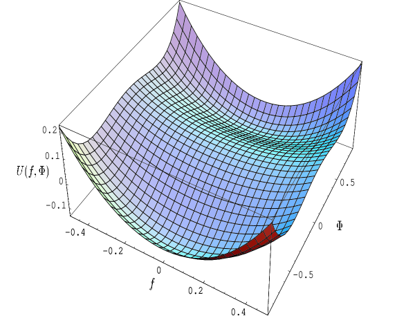
FIG. 1.: Potential $U(f,\Phi)$ for $g=1,\mu=1,m=1,\lambda=2$

There are three critical points: two points of the “minimum” type with the coordinates $(0,\pm\sqrt{\frac{m}{\lambda}})$, and one point of the “saddle” type with the coordinates $(0,0)$.

The system of equations (60) has a first integral, which is the conserved energy for the mechanical system with coordinates $f$ and $\Phi$

$$\dot{f}^{2}+\frac{g^{2}}{2}f^{4}+\frac{\dot{\Phi}^{2}}{2}+\lambda\frac{\Phi^{4}}{4}+\frac{\mu^{2}}{4}f^{2}+g^{2}f^{2}\Phi^{2}-\frac{m^{2}}{2}\Phi^{2}=const={\cal E}.$$ (62)

The nonlinear system (60) has many solutions, most of them can be obtained only numerically, and only few can be found analytically. As an example, we present here an analytical periodical solution expressed in terms of the elliptic Jacobi cosine $\mathop{\rm cn}\nolimits(x,k)$ and sine $\mathop{\rm sn}\nolimits(x,k)$ functions of the argument $x$ and the module $k$

$$f=\frac{1}{g}\sqrt{\left(1-\frac{g^{2}}{\lambda}\right)\left(\frac{\mu^{2}}{2}+2m^{2}\right)}\mathop{\rm cn}\nolimits(Bt,k),$$ (63)

$$\Phi=\sqrt{\frac{1}{\lambda}(\frac{\mu^{2}}{2}+2m^{2})}\mathop{\rm sn}\nolimits(Bt,k),$$ (64)

$$B^{2}=\frac{1}{4}\mu^{2}+\left(1-\frac{g^{2}}{\lambda}\right)\left(\frac{\mu^{2}}{2}+2m^{2}\right),$$ (65)

$$k^{2}=1-\frac{\frac{\mu^{2}}{2}+m^{2}}{B^{2}}.$$ (66)

The energy integral $\cal{E}$ for the solution (64) reads

$${\cal E}=\left(\frac{1}{g^{2}}-\frac{1}{\lambda}\right)\left(\frac{3}{2}m^{2}\mu^{2}+\frac{\mu^{4}}{4}+2m^{4}\right)+\frac{\mu^{2}}{4\lambda}\left(m^{2}+\frac{1}{4}\mu^{2}\right).$$ (67)

It is seen that this solution for $f$ and $\Phi$ is real, if $\lambda>g^{2}$. This evidently describes a regular periodic motion of the system around the saddle point of the potential, $f=0,\Phi=0$. The energy $\cal E$ in this case is positive, and well above the “saddle” point value of the potential $U(f,\Phi)=0$. This classical solution corresponds to the situation with restored symmetry of the YM–Higgs Lagrangian in quantum theory (for negative values of the energy ${\cal E}<0$ the effective “classical” particle should move near one of the nontrivial minima of the potential, which corresponds to broken symmetry of the YM–Higgs Lagrangian). It is easily seen that with growing $\mu,$ the energy increases (if $\lambda>g^{2}$). Thus, we may suppose that the presence of the CS term is conducive to restoration of symmetry. For energy values below the saddle point the solution tends to concentrate near one of the nontrivial minima of the potential (corresponding to breaking of symmetry). It should be expected that near the saddle point, trajectories of the system are highly unstable and the system should demonstrate stochastic behavior. In order to study this situation we should apply numerical methods of calculation. This will be done in the following section.

V Effective system with the potential $U(f,\Phi)$

Here, we will numerically analyze the behavior of the effective mechanical system with the potential $U(f,\Phi)$ given in (61) leading to the system of equations (60). Let us look for its numerical solutions for various choices of initial conditions. The functions $f(t)$ and $\Phi(t)$ for two choices of initial conditions are plotted in Figs. 2, 3. The curves are depicted for the following values of parameters $g=1,\mu=1,m=1,\lambda=2$.

FIG. 2.: System behavior for initial conditions $f_{0}=0.5,\dot{f}_{0}=0,\Phi_{0}=0.5,\dot{\Phi}_{0}=0$ and the set of parameter values $g=1,\mu=1,m=1,\lambda=2$

From the figures, one can see that there exist significantly differing types of motion for the system. Indeed, the trajectories correspond to three different types of motion: periodical, quasi-periodical and stochastic ones. The latter situation can be described by treating the interacting fields as an effective mechanical system with coordinates $\Phi,f$ and the Lagrangian

$$\ L=\dot{f}^{2}-\frac{\mu^{2}}{4}f^{2}-\frac{g^{2}}{2}f^{4}+\frac{\dot{\Phi}^{2}}{2}+\frac{m^{2}}{2}\Phi^{2}-\lambda\frac{\Phi^{4}}{4}-g^{2}f^{2}\Phi^{2}.$$ (68)

Let us now consider the term $-g^{2}f^{2}\Phi^{2}$ as a perturbation of the unperturbed system described by the Lagrangian

$$\ L_{0}=\dot{f}^{2}-\frac{\mu^{2}}{4}f^{2}-\frac{g^{2}}{2}f^{4}+\frac{\dot{\Phi}^{2}}{2}+\frac{m^{2}}{2}\Phi^{2}-\lambda\frac{\Phi^{4}}{4}.$$ (69)

FIG. 3.: System behavior for initial conditions $f_{0}=2.0,\dot{f}_{0}=0,\Phi_{0}=0.5,\dot{\Phi}_{0}=0$ and the set of parameter values $g=1,\mu=1,m=1,\lambda=2$

For the system with the Lagrangian $L_{0}$ all trajectories are either periodical or quasi-periodical, since variables $f$ and $\Phi$ are separately described by independent equations of the typical form $\dot{x}^{2}+ax^{2}+bx^{4}=const$ with the solutions $A\mathop{\rm cn}\nolimits(Bx,k)$ and $A\mathop{\rm sn}\nolimits(Bx,k)$ [22]. In order to describe the role of the perturbation, the KAM-theorem [26] can be applied which states that, if the perturbation is analytical and small enough, the part of the phase space, spanned by our system, can be divided into two regions of nonvanishing volumes, one of them being small as compared to the other and tending to zero in the limit of a vanishing perturbation. The larger region consists of invariant embedded toruses, densely covered with trajectories. In other words, for the majority of possible initial conditions, trajectories are of the Lissajous type, similar to the oscillator case. However, there exists a comparatively small region, corresponding to a small set of initial conditions, where trajectories are completely chaotic and may go astray from the neighboring “restricted” trajectories. This region has a non-zero volume and it may be called “instability region”.

To examine the trajectories in detail, let us follow [27] and seek numerical solutions with the Lagrangian $L$ and find intersections of trajectories and the plane $f=0$ under the condition $f^{\prime}>0$. Plotting the intersection points in the so called Poincaré surfaces of intersection, we can study the character of motion for the mechanical system equivalent to our interacting gauge and Higgs fields. In Fig. 4 we present such pictures for different values of ${\cal E}$. Each picture contains a set of trajectories with equal ${\cal E}$. If the set of intersection points for the given trajectory is restricted to a point, the motion is periodical; if they lie along the same curve, the motion is quasi-periodical.

FIG. 4.: $\Phi$ and $\frac{d\Phi}{dt}$ for $f=0,\dot{f}>0,{\cal E}=-0.1$ and $0.1$ ($g=1,\mu=1,m=1,\lambda=2$).

FIG. 5.: $\Phi$ and $\frac{d\Phi}{dt}$ for $f=0,\dot{f}>0,{\cal E}=0.5$ and $8.0$ ($g=1,\mu=1,m=1,\lambda=2$).

For the stochastic motion, the intersection points cover densely a finite area. The left picture in Fig. 4 corresponds to comparatively low energies, well below the “saddle” point. It is easily seen that all the trajectories form closed curves. According to KAM-theorem, this means that practically the entire phase space consists of toruses, which corresponds to quasiperiodical motion. For higher energies and larger perturbations (the right picture of Fig. 4), the situation is completely different: there arise regions of ergodic behavior, though there remain some small regions of toroidal structure. It should be clearly understood that dispersed points in Fig. 4 form one and the same trajectory which chaotically goes through almost the entire accessible domain of the phase space. For still higher energies the situation is different. The motion of the system again becomes more and more stabilized, which is seen in Figs. 4 and 5. The conclusion which follows from these numerical calculations is that near the saddle point the character of motion changes, corresponding to the symmetry breaking in the Lagrangian. The motion becomes more unstable and its stochastic character more pronounced when the energy is closer to the saddle point value.

We have also made use of the Toda-Brumer criterion [28] to find the critical energy $E_{c}$ such that for energies below $E_{c}$ no chaotic trajectories should be found. For our choice of parameters ($g=1,\mu=1,m=1,\lambda=2$)), we found $E_{c}=-\frac{5}{72}$. This value does not contradict our conclusion made with regard to numerical calculations and studies of Poincaré surfaces of section (see above). Unfortunately the Toda-Brumer criterion failed for critical energies above the saddle point.

VI Summary and conclusions

In this paper we have found an exact plane-wave solution of the field equations for the 3-d gauge field theory with a non-zero topological mass. The effective mass of the solution depends on two dimensional parameters of the model: the amplitude of the wave and the Chern-Simons topological mass. The plane-wave form of the solution becomes evident after applying the Lorentz boost. Thus, we obtain a nonlinear massive plane wave, and this is due not only to the nonlinear character of the gauge field equations, as was the case with the usual 4-d Yang-Mills equation [5], but also to the role of the massive Chern-Simons term. This term, on one hand, adds a positive contribution to the effective mass of the solution, and this makes the wave even heavier. On the other hand, it allows the energy density to become negative. Here, as a limiting case, we obtained a known static solution with the lowest energy possible for the class of solutions considered.

We were faced with another interesting situation, when we chose to include not only the CS term, but also a scalar Higgs field. A choice of the restrictive ansatz, similar to the one used in the previous Sections, now led us to an effective mechanical system with two degrees of freedom. We have demonstrated that for special initial conditions, the phase space trajectories are closed and regular. Chaotic behavior of the Yang-Mills theory in the 4-d space-time was discovered and studied by Matinyan and Savvidy (see [29], and [15] for reviews and discussions). In [14] the $d=2$ dimensional YM-Higgs theory was studied. There, the Higgs field was chosen to be an $SU(2)$ doublet. In that paper it was qualitatively demonstrated that spontaneous breakdown of gauge symmetry by the Higgs mechanism has a stabilizing effect on non-abelian gauge field dynamics. In our case, no spontaneous breaking of symmetry was initially assumed, rather the Higgs field was taken as a dynamical variable. Moreover, since we studied the $d=3$ case, we included the CS term into the consideration. Our result, based on numerical calculations, is that with growing energy $E$, the motion of the effective classical mechanical system first becomes more chaotic (in the vicinity of the critical saddle point of the potential), then with further growth of energy, again some regular components may appear.

The general physical conclusion of Matinyan and Savvidy [29] is that the Yang-Mills field system is not exactly solvable (otherwise, the trajectories would have a regular rather than chaotic form). This conclusion is confirmed in the present paper for the case of a 3-d gauge field model with a topological CS term and an additional interaction with a dynamical Higgs field. The presence of the CS topological mass in the 3-d case is conducive to the restoration of symmetry and to stabilizing the system.

REFERENCES

- [1] M.A. Shifman, Instantons in Gauge Theories, World Scientific, Singapore, 1994.
- [2] H.B. Nielsen and P. Olesen, Nucl. Phys. B61, 45 (1973).
- [3] G. ’t Hooft, Nucl. Phys. B79, 276 (1974).
- [4] S.Coleman, Phys. Lett., 70B, n. 1, 59 (1977).
- [5] G.Baseyan, S.Matinyan, and G. Savvidy, Pisma ZhETF 24, 641-644 (1979).
- [6] S.Matinyan, G. Savvidy, and N.Ter-Arutyunyan-Savvidy, ZhETF, 80, 830 (1981).
- [7] A.S.Vshivtsev and A.V.Tatarintsev , Ukrainskii Fiz. Zhurn., 33, n.2 , 165 (1988).
- [8] S.Deser, R.Jackiw and S.Templeton, Annals of Physics, 140, 372-411 (1982).
- [9] V.Ch.Zhukovsky and N.A.Peskov, One-loop energy corrections in the non-abelian gauge field theory in 2+1 dimensions, hep-th/9812221, Vest. Mosk. Univ., Fiz. Astr., N2, 60 (1999).
- [10] A.A.Sokolov, I.M.Ternov, V.Ch.Zhukovsky, and A.V.Borisov, Gauge Fields (in Russian), Moscow, Moscow University Press, 1986.
- [11] V.A.Rubakov, Classical Gauge Fields (in Russian), published by the Inst. of Nucl. Research, parts 1, 2, 3, Moscow, 1996.
- [12] T.S.Biro, S.G.Matinyan, and B.Mueller. Chaos and Gauge Field Theory. Lecture Notes in Physics, Vol. 56, World Scientific, 1994.
- [13] B.Chirikov and D.Shepelyanski,JETP Letters, 34, 163 (1981); Sov. J. Nucl. Phys., 36, 908 (1982); B.Chirikov, Physics Reports, 75, 287 (1981).
- [14] S.Matinyan et al., JETP Letters, 34, 590 (1981);
- [15] G.K. Savvidy, Nucl. Phys. B246, 302 (1984).
- [16] W.Steele et al., Phys.Rev. D 33, 1174 (1986).
- [17] W.Steele et al., Phys. Rev. A33, 2131 (1986).
- [18] B.Dey et al., Int. J. Mod. Phys, A8, 1755 (1993).
- [19] E.Haller et al., Phys.Rev.Lett, 52, 1665 (1984).
- [20] J.P.Blaizot et al., Phys.Rev.Lett, 72, 3317 (1994).
- [21] A.Giasanti et al., Phys.Rev., D 38, 1352 (1988).
- [22] G.Korn and M.Korn, Mathematical Handbook for Scientists and Engineers, New York, 1968.
- [23] L.D.Faddeev, hep-th/9807069.
- [24] S.P.Novikov, Theory of Solitons: Method of Inverse Problem (in Russian), Moscow, 1980.
- [25] R.Rajaraman, An Introduction to Solitons and Instantons in Quantum Field Theory, North-Holland Publishing Company, Amsterdam - New York - Oxford, 1982.
- [26] A.N.Kolmogorov, DAN SSSR, 98, 527 (1954). V.I.Arnold, Uspekhi Mat. Nauk, 18, 13 (1963). J.Moser, Nachr. Acad. Wiss. Göttingen, Math. Phys., K1, 11 a, 1 (1962); see also V.I.Arnold, Mathematical Methods of Classical Mechanics (in Russian), Moscow, 1974.
- [27] M.Henon and C.Heiles, Astron. Journ., 69, 73 (1964).
- [28] M. Toda, Phys. Lett., A48, 335 (1974); P. Brumer and J.W. Duff, J. Chem. Phys., 65, 3566, (1976).
- [29] S.G.Matinyan, Fiz. Elem. Chast. Atom. Yadra, 16, 522 (1985).