Abstract

Giant gravitons in ${\rm AdS}_{5}\times{\rm S}^{5}$, and its orbifolds, have a dual field theory representation as states created by chiral primary operators. We argue that these operators are not single-trace operators in the conformal field theory, but rather are determinants and subdeterminants of scalar fields; the stringy exclusion principle applies to these operators. Evidence for this identification comes from three sources: (a) topological considerations in orbifolds, (b) computation of protected correlators using free field theory and (c) a Matrix model argument. The last argument applies to ${\rm AdS}_{7}\times{\rm S}^{4}$ and the dual $(2,0)$ theory, where we use algebraic aspects of the fuzzy 4-sphere to compute the expectation value of a giant graviton operator along the Coulomb branch of the theory.

1 Introduction

There is a remarkable mechanism in string theory for regulating potential divergences and singularities: increasing the energy of a state often causes it to expand, thereby softening its interactions. An example of this effect is the “giant graviton” [1] of the ${\rm AdS}_{5}\times{\rm S}^{5}$ solution of IIB supergravity. Here the Myers effect [2] causes a graviton having very large angular momentum on an ${\rm S}^{5}$ with nonzero Ramond-Ramond five-form flux to expand into a spherical D3-brane, whose size is related to its angular momentum. This phenomenon suggests that one of the basic symmetries of nature — reparametrization invariance — has a little-understood generalization in the presence of Ramond-Ramond fluxes. Apparently, at very high energies in some backgrounds, the graviton, the “gauge boson” of reparametrization invariance, becomes a macroscopic extended object. In view of this, it is clearly important to study the properties of giant gravitons and their representation in dual field theories.

${\rm AdS}_{5}\times{\rm S}^{5}$ is dual to to ${\cal N}=4$ SYM [3]. The standard map between these dual descriptions identifies single giant gravitons with single-trace chiral operators of large R-charge in the field theory. The evidence for this identification, besides the matching of charges, is two-fold. First, at low R-charge, the number of traces in an operator counts particle number in the dual gravity Fock space. If we identify a giant D3-brane as a single graviton, then it should be created by a single-trace operator. Second, there is a bound on the R-charge of single-trace operators in the Yang-Mills theory. This neatly matches the bound on the angular momentum of a giant graviton, which arises because a spherical D3-brane on ${\rm S}^{5}$ has a size that is bounded by the ${\rm S}^{5}$ radius.

In this paper, we show that the identification of giant gravitons as single-trace operators in the dual field theory cannot be correct. Rather, we will present evidence that large giant gravitons are dual to states created by a family of subdeterminants. (A subdeterminant of an $N\times N$ matrix $X^{a}_{b}$ is

$$\det{}_{k}X={1\over k!}\epsilon_{i_{1}\cdots i_{k}a_{1}\cdots a_{N-k}}\epsilon^{j_{1}\cdots j_{k}a_{1}\cdots a_{N-k}}X^{i_{1}}_{j_{1}}\cdots X^{i_{k}}_{j_{k}}\,.$$

So ${\rm det}_{N}$ is the same as the determinant.) These subdeterminants have a bounded R-charge, with the full determinant saturating the bound. Once again, the bound on the R-charge is the field theory explanation of the angular momentum bound for giants.

In Sec. 2 we explain how the failure of the planar approximation for correlation functions of large dimension operators invalidates the single particle/single trace correspondence. This makes problematic the identification of giant gravitons as single-trace operators. In Sec. 3 we identify maximal-sized giant gravitons with determinants, using evidence from various orbifolds of ${\cal N}=4$ Yang-Mills theory and corresponding dual gravities. In Sec. 4 we argue that less-than-maximal giant gravitons are created by subdeterminants. Sec. 5 presents a Matrix theory argument which shows that giant gravitons in ${\rm AdS}_{7}\times{\rm S}^{4}$ are created by the analog of subdeterminants in the $(2,0)$ theory, by relating dynamical aspects of giant gravitons to algebraic aspects of the fuzzy 4-sphere. We conclude, in Sec. 6, with comments on future directions.

Parts of Sec. 5 were developed in collaboration with Moshe Rozali.

2 Giant gravitons are not traces

The best semiclassical description of a graviton with large momentum on the ${\rm S}^{5}$ of ${\rm AdS}_{5}\times{\rm S}^{5}$ is in terms of a large D3-brane wrapping a 3-sphere and moving with some velocity[1]. This is the giant graviton. The transition from a graviton mode in a spherical harmonic to a macroscopic brane is explained by the Myers effect [2] in the presence of flux on the ${\rm S}^{5}$. In ${\rm AdS}_{5}\times{\rm S}^{5}$, the radius of the spherical D3-brane is $\rho^{2}=lR^{2}/N$, where $l$ is the angular momentum on the ${\rm S}^{5}$ of the state, $R$ is the radius of the sphere, and $N$ the total 5-form flux through the 5-sphere.

Our first point is that giant gravitons in the bulk supergravity description are not created by single-trace operators in the conformal field theory, as usually stated. There are strong arguments that a graviton with small angular momentum is created by a single-trace operator, and that a state with $p$ gravitons is created by a product of $p$ single-trace operators. These arguments rely on the special factorization properties of correlation functions in large-$N$ gauge theories. But factorization breaks down for operators with dimension of order $N$ — and thus for chiral operators with R-charge of order $N$ — so there are no such arguments for states containing giant gravitons.

For example, consider two states with equal total angular momentum and energy, but with that momentum and energy partitioned differently among one or more giant gravitons. These states are classically different, and should represent orthogonal states in the Hilbert space of the theory. However, candidate multi-trace operators with the correct charges do not generate orthogonal states (at least, the familiar arguments of approximate orthogonality fail).

2.1 Some basic tools

In this paper we will identify field theory operators that correspond to giant gravitons on the gravity side of the AdS/CFT correspondence. We will write these composite operators in terms of the fundamental fields in the Lagrangian, a description that is useful at weak coupling. Strictly speaking the AdS/CFT correspondence applies at strong field theory coupling and so the operators we identify should be extrapolated to this regime. Since they are chiral, there are no significant problems with this extrapolation. We will discuss two types of systems: ${\cal N}=4$ theories, and nonperturbative fixed points of ${\cal N}=1$ theories (which can be constructed as infrared fixed points of weakly-coupled theories.)

${\cal N}=4$ theories:

The chiral primary operators of 4d, ${\cal N}=4$, $SU(N)$ Yang-Mills theory are in the $(0,l,0)$ representation of the $SU(4)\sim SO(6)$ R-symmetry group. These operators, which may have one or more traces over gauge indices, have protected dimensions $l\geq 2$. Single-trace chiral primaries are of the form $\mathop{\rm Tr}\,(X^{i_{1}}X^{i_{2}}\cdots X^{i_{l}})$, where each scalar $X^{i}$ is a vector of SO(6), while the product of scalars forms a symmetric traceless representation of this group. These operators generate the chiral “ring” of the theory. There is a bound $l\leq N$ for the single-trace chiral primaries, because all higher $l$ operators can be written as sums of products of lower dimension operators.

We are also interested in the $SO(2N)$, ${\cal N}=4$ theory. The spectrum of single-trace operators is similar, except that only the $(0,2l,0)$ representations appear, and there is one additional representation needed to generate the chiral ring. The corresponding operator is a Pfaffian of the scalar fields, which are antisymmetric $2N\times 2N$ matrices.

In ${\cal N}=1$ supersymmetric language, the ${\cal N}=4$ theory consists of a vector multiplet and three chiral multiplets $\Phi_{\mu}=X_{\mu}+iX_{\mu+3}$, $\mu=1,2,3$, all in the adjoint representation of the gauge group. The $SO(6)$ R-symmetry is partially hidden by the ${\cal N}=1$ notation. Only a $U(1)$ R-symmetry and the $SU(3)$ that rotates the $\Phi_{\mu}$ are visible. The chiral operators described above include operators of the form $\mathop{\rm Tr}(\Phi^{\mu_{1}}\Phi^{\mu_{2}}\cdots\Phi^{\mu_{n}})$ (symmetrized over the $SU(3)$ indices). However, there are chiral operators of the ${\cal N}=4$ theory which appear to be non-chiral in the ${\cal N}=1$ notation. This is because a short representation of the ${\cal N}=4$ algebra includes both short and long representations of a ${\cal N}=1$ subalgebra. In the rest of this paper, we will use the ${\cal N}=1$ language. Also, for simplicity, we will examine R-charges in a single $U(1)$ and will suppress the index $\mu$.

In these theories $g_{ym}^{2}$ is a marginal coupling constant (and it couples to some operator $O_{marg}$). We will only be studying chiral operators and extremal correlation functions, for which there are powerful non-renormalization theorems. If $O_{p}$ is any scalar chiral primary operator in the $(0,l,0)$ representation (whether a single trace or a multi-trace operator), then extremal correlators are correlators of the form

$$<O_{p_{1}}\cdots O_{p_{n}}>,\ \ \ p_{1}=p_{2}+\cdots p_{n}.$$ (2)

These are independent of the coupling.. The result is that we can compute these correlators reliably at weak coupling.

For the most part we will use an even more restricted class of correlators which are just 3 point functions of chiral primaries. In this case all such 3 point functions, irrespectively of whether they are extremal or not, are not renormalized .

These non-renormalization theorems were first discussed in [7], extended in [8], extensively checked by supergravity and field theory computations in [9], and was finally proven in [10]. Whereas most of the references [7, 8, 9] focussed on single-trace operators, [10] relies, as a superspace proof has to, only on algebraic properties of the operators. Hence it applies to all primaries operators in chiral $(0,l,0)$ representations, whether they are defined as single-trace at weak coupling or not.

We will also be referring to finite ${\cal N}=2$ and ${\cal N}=1$ theories. In the ${\cal N}=2$ case, the non-renormalization theorem applies just as well [10]. In the ${\cal N}=1$ case, there is no exact non-renormalization theorem, although one expects some remnant of it at large $N$ for theories obtained by orbifolding ${\cal N}=2$ or $4$ theories.

Fixed points of ${\cal N}=1$ theories:

We will also encounter ${\cal N}=1$ fixed point theories that can be defined by starting with a weakly-coupled Lagrangian description in the UV and flowing to a strongly-coupled fixed point in the IR. The operators are defined in the UV using fundamental fields in the Lagrangian, and the IR objects are particles or branes on $AdS\times X$. In this case, there is no non-renormalization theorem for correlation functions and operators mix. Nevertheless, we will consider operators corresponding to topologically stable objects on $AdS\times X$. Such operators are the lowest dimension objects carrying certain discrete quantum numbers. Hence their operator mixing is extremely limited. We will also consider products of operators of this type. Since these are products of chiral operators no new renormalizations or operator mixings are introduced.

2.2 Small angular momenta

According to the standard AdS/CFT dictionary, states created by the chiral primary operators of the ${\cal N}=4$, $SU(N)$ theory (more precisely, generators of the chiral ring) map into modes of fields of IIB supergravity in the background ${\rm AdS}_{5}\times{\rm S}^{5}$. The SO(6) isometries of the sphere appear as R-symmetries of the AdS theory as well as the dual CFT. Spherical harmonics on the sphere lead, upon Kaluza-Klein reduction to AdS, to a tower of massive fields transforming in the $(0,l,0)$ representations of SO(6). These fields have a Fock space of single and multi-particle states in AdS which form an orthogonal basis. In the standard AdS/CFT map, particle number in AdS is mapped into the number of traces in the operator creating the dual field theory state. It is instructive to examine the rationale behind the identification of these quantum numbers.

In general, a state created by a composite operator like $\mathop{\rm Tr}X^{l}$ need not be orthogonal to states created by other gauge invariant operators with the same dimension. For example,

$$\langle\mathop{\rm Tr}(\Phi^{l})^{\dagger}\,(\mathop{\rm Tr}(\Phi^{l-2})\,\mathop{\rm Tr}\Phi^{2})\rangle\neq 0$$ (3)

However, if the rank of the gauge group $N$ is large compared to $l$, there is approximate orthogonality because of well-known properties of this limit. For example, let

$${\cal O}_{1} = \mathop{\rm Tr}(\Phi^{l})\,,$$ (4)

$${\cal O}_{2} = \mathop{\rm Tr}\Phi^{l_{1}}\mathop{\rm Tr}\Phi^{l_{2}}\,\,\,\,\,\,\,\,\,\,\,\,\,\,\,\,\,l_{1}+l_{2}=l$$ (5)

Then,

$$\langle\,{\cal O}_{1}^{\dagger}\,{\cal O}_{1}\,\rangle\sim lN^{l},$$

$$\langle\,{\cal O}_{2}^{\dagger}\,{\cal O}_{2}\,\rangle\sim l_{1}l_{2}N^{l}$$

where we have left out the space-time dependence. To compute this 2-point function in the large-$N$ limit, we have recognized that planar diagrams dominate and have done the $N$-counting by looking at the free diagrams in Fig. 1A and B. With these results we can compute the normalized 2-point function of two different operators in the planar approximation. The $N$-counting can again be understood from the free diagram in Fig. 1C:

$$\frac{\langle\,{\cal O}_{1}^{\dagger}\,{\cal O}_{2}\,\rangle}{\sqrt{\langle\,{\cal O}_{1}^{\dagger}\,{\cal O}_{1}\,\rangle}\sqrt{{\langle\,{\cal O}_{2}^{\dagger}\,{\cal O}_{2}\,\rangle}}}\sim\frac{\sqrt{l_{1}\,l_{2}\,l}}{N}$$ (6)

By the state-operator correspondence in CFTs, this implies that the states created by ${\cal O}_{1}$ and ${\cal O}_{2}$ are orthogonal in the $N\rightarrow\infty$ limit. In general, operators with the same dimension but with different numbers of traces create states that are orthogonal at large $N$, as in (6). This suggests that the number of traces is a conserved quantum number at large $N$. Furthermore, disconnected graphs dominate in two-point functions of multi-trace operators, so it appears that a product of single-trace operators gives a state which is a direct product of noninteracting single particle states. Altogether, this leads to the conclusion that the number of particles in AdS should be mapped into the number of traces in the CFT.

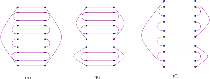
Figure 1: Planar diagrams for :(A) $\langle{\cal O}_{1}{\cal O}_{1}\rangle$ (there are $l$ such diagrams from cyclic permutations inside the Trace), (B) $\langle{\cal O}_{2}{\cal O}_{2}\rangle$ (there are $l_{1}\,l_{2}$ such diagrams), (C) $\langle{\cal O}_{1}{\cal O}_{2}\rangle$ (there are $l_{1}\,l_{2}\,l$ such diagrams).

2.3 Failure of planarity and orthogonality of traces

It is well known that the dominance of planar graphs at large $N$ is only true for operators whose dimensions are small. For correlation functions of operators whose dimensions scale sufficiently fast with $N$, it fails badly [11]. It is readily checked that when $l$ is sufficiently large, combinatorial factors in non-planar diagrams can overwhelm the usual suppression by powers of $1/N^{2}$. When $l$ is large, even the planar calculation (6) does not show orthogonality of states created by operators with different numbers of traces. For example, (6) shows that the planar contribution to the two-point function scales as:

$$l=O(N),\,\,l_{1}=O(N),\,\,l_{2}=O(1)~{}~{}~{}~{} \longrightarrow ~{}~{}~{}~{}\frac{\langle\,{\cal O}_{1}^{\dagger}\,{\cal O}_{2}\,\rangle}{\sqrt{\langle\,{\cal O}_{1}^{\dagger}\,{\cal O}_{1}\,\rangle}\sqrt{{\langle\,{\cal O}_{2}^{\dagger}\,{\cal O}_{2}\,\rangle}}}\sim O(1)$$ (7)

$$l\sim N,\,\,l_{1}=l_{2}=l/2~{}~{}~{}~{} \longrightarrow ~{}~{}~{}~{}\frac{\langle\,{\cal O}_{1}^{\dagger}\,{\cal O}_{2}\,\rangle}{\sqrt{\langle\,{\cal O}_{1}^{\dagger}\,{\cal O}_{1}\,\rangle}\sqrt{{\langle\,{\cal O}_{2}^{\dagger}\,{\cal O}_{2}\,\rangle}}}\sim\sqrt{N}$$ (8)

It is rather unlikely that the large non-planar contributions to this two-point function will conspire to cause it to cancel at large $N$, although they should correct the apparently non-unitary growth of (8), in conjunction with non-perturbative effects. The salient point is that although it is hard to do an exact computation of the two-point function even in free field theory, there is no reason to expect that states created by high dimension operators with different numbers of traces are orthogonal. “Trace number” is simply not a good quantum number. A consequence of this for the AdS/CFT duality is that we cannot map CFT trace number into particle number in an AdS Fock space for states of high dimension.

2.4 Scales in gravity, gauge theory and giants

The ground state wavefunction for a scalar field on ${\rm AdS}_{5}$ arising from a mode with large angular momentum $l$ on ${\rm S}^{5}$ is [12]:

$$\psi\propto e^{-i\,l\,t}{1\over(1+r^{2}/R^{2})^{l/2}}$$ (9)

Here $r$ is a radial coordinate in AdS, $R=(g_{s}N\alpha^{\prime 2})^{1/4}$ is the curvature scale, and $l$ is the angular momentum on ${\rm S}^{5}$. The effective mass of the scalar field, induced by the large angular momentum, is $(mR)^{2}\sim l^{2}$. The typical size of this wavefunction decreases as $l$ increases, so that when $l>(g_{s}N)^{1/2}$ it has a width smaller than the string scale and therefore cannot be trusted. Equivalently, semiclassical supergravity calculations can only trusted for particles with masses below the string scale ($l<(g_{s}N)^{1/2}$) and the Planck scale ($l<N^{1/2}$). Another criterion that can be applied is to require that the wavelength of modes on the ${\rm S}^{5}$ is larger than the string length or Planck length. This gives bounds $l<(g_{s}N)^{1/4}$ and $l<N^{1/4}$ respectively. It is clear that for such small values of $l$ the two-point function (6) approaches zero, the planar approximation is valid, and the standard mapping of one-particle states to single-trace operators continues to hold.

In [1], it was argued that a large class of states with large angular momenta should be described by spherical, BPS D3-branes which are extended on ${\rm S}^{5}$ but localized at a point on ${\rm AdS}_{5}$. Such spherical brane configurations on an ${\rm S}^{5}$ of radius $R$ are supported by the angular momentum $l$ and the $N$ units of background flux. They have a radius $\rho^{2}=lR^{2}/N$. Since $\rho$ cannot exceed $R$, there is a bound on the angular momentum $l\leq N$. The semiclassical description of giants shows that there is a clear distinction between single- and multi-giant states, and that, despite being non-perturbative objects, they interact weakly with perturbative gravitons and with each other.

A giant graviton can be treated as a non-perturbative state in weakly coupled string theory when its size $\rho$ exceeds the Planck scale ($l_{p}^{8}=l_{s}^{8}g_{s}^{2}$). After applying the AdS/CFT dictionary, this requires that $l>N^{1/2}$. The dual CFT two-point function (6) shows that the planar approximation for correlation functions, and with it the argument for orthogonality of multi-trace operators, breaks down at least when $l>N^{2/3}$. Therefore, since single- and multi-giant states are clearly orthogonal at weak coupling, large giants cannot be described by single- and multi-trace chiral primaries of large R-charge. Indeed, traces can be a good description at most when $l<N^{2/3}$. What is more, since trace number is not a good quantum number at large $l$, the bound on the R-charge of single trace chiral primaries cannot be mapped meaningfully to the angular momentum bound for giant gravitons.

The Puzzle:

Nevertheless, giant gravitons exist as semiclassical entities. They are non-perturbative, BPS brane states, and we expect configurations of giants with the same total angular momentum but different numbers of branes to be orthogonal. Brane number, unlike particle number, makes sense from the point of view of gravity at these high energies. Although single- and multi-trace chiral primaries make states that carry the same charges as the giant gravitons, we cannot map “trace number” to brane number since the former is not a good quantum number. As a corollary, we cannot relate the bound on the angular momentum of single giants to the bound on the charge of single-trace operators. What operator, then, makes a giant graviton in the CFT? And whence the bound on the angular momentum?

3 Biggest giants should be determinants

The resolution of these questions begins with the simple observation that we have seen D3-branes in the AdS/CFT correspondence before. Specifically, topologically non-trivial D3-branes play an important role in theories in which the five-sphere is orbifolded, or replaced with another space with non-trivial three-cycles, such as $T^{1,1}$.

A BPS D3-brane wrapped on such a 3-cycle corresponds to an operator in the CFT of dimension $\sim N$. Such a state carries a topological charge in addition to its angular momentum, and is the lightest object with this charge. Unlike non-topological BPS gravitons, which are neutrally stable with respect to states with multiple BPS gravitons, these wrapped D3-branes cannot split into multi-brane or brane-graviton states. The corresponding chiral operator in the CFT is therefore easy to identify, since it must be the lowest-dimension chiral operator with a certain conserved charge corresponding to the wrapping charge of the brane. In many cases this charge is a baryon number, and the operator is baryon-like.

In each case, there are also chiral operators with the cancelling topological charge. A product of chiral operators, each of which carries topological charge but whose combination is neutral, is naturally associated to a combination of wrapped D3-branes each of which is topologically nontrivial but which when joined together are topologically trivial. Such D3-branes are in the same class as the giant gravitons of [1], which are topologically-trivial BPS brane states that are dynamically stabilized by their angular momentum. As we will see, these products of topologically-charged chiral operators are always determinants of neutral combinations of the matrix-valued fields in the CFT. These determiniants carry the maximum angular momentum on the space, and are therefore candidates for the maximal giant gravitons, those at the edge of the angular momentum bound.

We begin with the most carefully studied case, the near-horizon region near $N$ D3-branes on a ${Z_{3}}$ orbifold.

3.1 The $Z_{3}$ orbifold

Gravity:

The sphere in the ${\rm AdS}_{5}\times{\rm S}^{5}$ solution of IIB gravity can be parametrized in complex coordinates $(z_{1},z_{2},z_{3})$ as the solution to $|z_{1}|^{2}+|z_{2}|^{2}+|z_{3}|^{2}=R^{2}$. Consider the $Z_{3}$ orbifold:

$$z_{i}\sim z_{i}\,\omega~{}~{}~{}~{};~{}~{}~{}~{}\omega=e^{2\pi i/3}\,.$$ (10)

This orbifold has no fixed points, and has non-trivial 3-cycles on which D3-branes can be wrapped. Specifically,

$$H_{3}({\rm S}^{5}/Z_{3},Z)=Z_{3}\,.$$ (11)

This torsion class is generated by an ${\rm S}^{3}/Z_{3}$ which is defined, up to $U(3)$ transformations of the $z_{i}$, by $z_{3}=0$. Branes wrapped on such cycles carry a $Z_{3}$ valued D3-brane charge.

The first integral homology group of the orbifold is

$$H_{1}({\rm S}^{5}/Z_{3},Z)=Z_{3}\,.$$ (12)

This torsion class is generated by an ${\rm S}^{1}/Z_{3}$ given, up to $U(3)$ transformations, by $z_{2}=z_{3}=0$. Fundamental strings and D-strings can be wrapped on this cycle giving twisted sectors with a $Z_{3}$ valued charge. The same cycle leads to a non-trivial fundamental group $\pi_{1}({\rm S}^{3}/Z_{3})=Z_{3}$ on the wrapped D3-brane worldvolume.

Discrete Wilson lines can be chosen on the worldvolumes of branes wrapped on cycles with nontrivial $\pi_{1}$, leading to a set of D-brane bound states [13]. In the present case, where $\pi_{1}=Z_{3}$ is discrete, Abelian and finite, there are Wilson lines, with three possible monodromies $1$, $\omega$ and $\omega^{2}$ around the nontrivial 1-cycle. By turning on such Wilson lines, we get three discrete vacua for a 3-brane wrapped once around ${\rm S}^{3}/Z_{3}$. We will call these states, which are cyclically permuted by the quantum $Z_{3}$ symmetry of the orbifold, $|U\rangle$, $|V\rangle$ and $|W\rangle$. Following [13], we can take linear combinations of these vacua to get eigenstates of the quantum $Z_{3}$ which carry definite fundamental string charge:

$$|U\rangle+|V\rangle+|W\rangle~{}~{}~{};~{}~{}~{}|U\rangle+\omega\,|V\rangle+\omega^{2}\,|W\rangle~{}~{}~{};~{}~{}~{}|U\rangle+\omega^{2}\,|V\rangle+\omega\,|W\rangle\,.$$ (13)

These vacua are bound states of the wrapped D3-brane with a twisted sector string. Conversely, the states $|U\rangle$, $|V\rangle$ and $|W\rangle$ carry indefinite F-string charge, but carry definite D1-brane charge in accord with the non-commutation of ‘t Hooft and Wilson lines, as discussed in [14].

We are interested in the largest dynamically stable giant graviton. For concreteness, consider only operators which are charged under a $U(1)$ part of the global $U(3)$ symmetry which rotates just the $z_{1}$ coordinate. The corresponding giant gravitons are D3-branes which wrap an ${\rm S}^{3}$ (${|z_{2}|}^{2}+{|z_{3}|}^{2}=\rho^{2}$), and rotate along the circle ${|z_{1}|}^{2}=R^{2}-\rho^{2}$. The radial size of the spherical brane is determined by $\rho^{2}=lR^{2}/N$ [1], where $R$ is the radius of the ${\rm S}^{5}/Z_{3}$. On the covering space (${\rm S}^{5}$), we can consider three branes at image points under $Z_{3}$. To reach the maximal size we take $l\rightarrow N$, getting three D3-branes at $z_{1}=0$. On the covering space these three branes wrap the 3-sphere $|z_{1}|^{2}+|z_{2}|^{2}=R^{2}$, which is modded out by the action of the $Z_{3}$ to become an ${\rm S}^{3}/Z_{3}$ in the orbifold. To study maximal giant gravitons we should therefore examine topologically trivial states that are triply-wrapped on the ${\rm S}^{3}/Z_{3}$ inside ${\rm S}^{5}/Z_{3}$.

A D3-brane that is triply-wrapped on ${\rm S}^{3}/Z_{3}$ is topologically trivial and should therefore carry no charge under the quantum $Z_{3}$ that permutes $|U\rangle$, $|V\rangle$ and $|W\rangle$. We can construct such a state by placing all three kinds of topologically protected branes that were discussed above on the ${\rm S}^{3}/Z_{3}$ at the same time. The resulting state, which we will call $|UVW\rangle$, has a $U(3)$ Wilson line with monodromy ${\rm diag}(1,\omega,\omega^{3})$. This can be written, after a change of basis, as the permutation matrix

$$\pmatrix{0&1&0\cr 0&0&1\cr 1&0&0}\,,$$ (14)

as appropriate to a triply-wrapped brane.

Although such a brane is topologically trivial, it is stabilized by dynamical effects. This can be seen by examining the arguments in [1] that originally established the existence of giant gravitons. Those authors used the Born-Infeld action to demonstrate that a spherical brane with an angular momentum $l$ on ${\rm S}^{5}$ is stabilized by the flux. The maximal giant graviton (of radius $R$) in their case is actually stationary and acquires all its angular momentum from interaction with the flux via the Chern-Simons term in its action. The Born-Infeld calculation of [1] can be repeated in our case by observing that it is locally unchanged on the worldvolume of the orbifolded brane. Therefore, the BPS condition relating energy and charge follows automatically.

The dynamically stabilized state that we have constructed is a maximal size giant graviton of the orbifold theory, since the three ${\rm S}^{3}/Z_{3}$ surfaces from which it is constructed have the maximum radius ($R$) that a three cycle can have on the ${\rm S}^{5}/Z_{3}$. We will show how this giant is described in the dual field theory.

Field Theory:

${\rm AdS}_{5}\times{\rm S}^{5}/Z_{3}$ is the near horizon limit of $3N$ D3-branes placed at the fixed point of ${\cal C}^{3}/Z_{3}$ [14, 15]. The resulting ${\cal N}=1$ field theory on the D-branes has a gauge group $SU(N)\times SU(N)\times SU(N)$. There are chiral matter superfields $U_{\mu}$, $V_{\mu}$ and $W_{\mu}$, $\mu=1,2,3$ each transforming as a bifundamental of a pair of these $SU(N)$ factors and as a singlet of the third. The theory has a $U(1)$ ${\cal N}=1$ R-symmetry, and an ordinary $SU(3)$ global symmetry which rotates the index $\mu$. This $U(3)$ is the subgroup of the $SO(6)$ ${\cal N}=4$ R-symmetry which survives the orbifold projection; it rotates the complex coordinates $z_{i}$ of ${\cal C}^{3}/Z_{3}$.

Detailed identification of the states and symmetries of this theory with string theory on ${\rm AdS}_{5}\times{\rm S}^{5}/Z_{3}$ was carried out in [14]. These authors argue that the D3-brane states that are singly-wrapped on ${\rm S}^{3}/Z_{3}$ — $|U\rangle$, $|V\rangle$ and $|W\rangle$ — are created from the CFT vacuum by the gauge invariant “dibaryon” operators

$$\det U,\,\,\det V,\,\,\det W$$ (15)

where

$$\det U=\epsilon_{i_{1}\cdots i_{N}}\,\epsilon^{j_{1}\cdots j_{N}}\,U^{i_{1}}_{j_{1}}\cdots U^{i_{N}}_{j_{N}}\,.$$ (16)

Note that $i_{s}$ and $j_{s}$ are indices in different $SU(N)$ factors. We have left out the $U(3)$ index $\mu$. Appropriate symmetrization over the latter index would be needed to construct different $U(3)$ representations, but we will not need to consider the most general giant; we can instead take all $\mu=1$.

The maximal giant graviton of the orbifold theory is the triply-wrapped brane state $|UVW\rangle$. This is created by the operator

$$\det U\,\det V\,\det W\equiv\det(UVW)=\epsilon_{i_{1}\cdots i_{N}}\,\epsilon^{{\bar{i}}_{1}\cdots{\bar{i}}_{N}}\,(UVW)^{i_{1}}_{{\bar{i}}_{1}}\cdots(UVW)^{i_{N}}_{{\bar{i}}_{N}}\,.\,.$$ (17)

Note that $i_{s}$ and ${\bar{i}}_{s}$ are in the same $SU(N)$ factor. Thus, the BPS D3-brane wrapped on the largest possible non-topological 3-cycle is created in the dual CFT by a determinant of a topologically-neutral combination of matrix-valued fields.

3.2 Other examples

SO(2N):

The $SO(2N)$, ${\cal N}=4$ Yang-Mills theory is dual to ${\rm AdS}_{5}\times{\cal R}{\cal P}^{5}$. The theory has six scalar fields $X_{i}$ in the adjoint representation; these are antisymmetric tensors in color space. Consider the complex combination $\Phi=X_{1}+iX_{2}$. There is a gauge-invariant, symmetric combination of $N$ of these tensors with a single $2N$-index epsilon tensor. This is the Pfaffian of $\Phi$, ${\rm Pf}(\Phi)$, which was identified by [11] as creating the state with a single BPS D3-brane wrapped on the nontrivial three-cycle of ${\cal R}{\cal P}^{5}$, and carrying a conserved $Z_{2}$ quantum number. The maximal giant graviton is the topologically trivial brane state which wraps twice the non-trivial cycle. Again, this can be understood by taking a near-maximal giant graviton with the quantum numbers of $\Phi^{l}$. This is a D3-brane wrapping an ${\rm S}^{3}$ and rotating at ${|\Phi|}^{2}=R^{2}(1-l/N)$. As $l\rightarrow N$, $\rho\rightarrow 0$ and we obtain a brane doubly wrapping the ${\cal R}{\cal P}^{3}$ at $\Phi=0$. This doubly wrapped D3-brane is topologically unstable but is dynamically stable following [1]. Since

$${\rm Pf}(\Phi)\,{\rm Pf}(\Phi)=\det\Phi\,,$$ (18)

we see that the maximal giant graviton of the $SO(2N)$ theory should be identified with $\det\Phi$.

$Z_{2}$ orbifold:

The finite $SU(N)\times SU(N)$, ${\cal N}=2$ gauge theory with two hypermultiplets $A_{i},B_{i}$ ($i=1,2$) in the bifundamental representation is dual to ${\rm AdS}_{5}\times{\rm S}^{5}/Z_{2}$ [15]. This ${\cal N}=2$ theory has oriented three-cycles whose winding number takes values in $Z$, and which have two possible orientations. A D3-brane wrapped on a cycle with one orientation is a dibaryon created by $\det A$, suppressing global symmetry quantum numbers for the moment. The topological charge is dibaryon-number, and it is integer-valued, as there is no way to reduce the operator $(\det A)^{n}$ to sums of other operators. A wrapped D3-brane in the opposite orientation is the diantibaryon $\det B$, carrying opposite topological charge. A di-baryon-antibaryon state is wrapped doubly and non-topologically around the equator of ${\rm S}^{5}/Z_{2}$, but is dynamically stabilized following the discussion above. This is a maximal size giant graviton of the orbifold theory. Clearly, since

$$\det A\,\det B=\det(AB)\,.$$ (19)

the maximal giant graviton is again identified with a determinant.

The conifold:

There is a conformal $SU(N)\times SU(N)$, ${\cal N}=1$ gauge theory with chiral multiplets $A_{i},B_{j}$ ($i,j=1,2$) in the bifundamental and a antibifundamental representation and with superpotential $W={\rm tr\ }(A_{i}B_{j}A_{k}B_{\ell})\epsilon^{ik}\epsilon^{j\ell}$. This is dual to ${\rm AdS}_{5}\times T^{1,1}$, the base of the conifold treated as a cone [16, 17]. Like the $Z_{2}$ orbifold, $T^{1,1}$ has 3-cycles with integer winding numbers and two orientations. D3-branes wrapped in the two orientations give rise to dibaryons and antidibaryons created by $\det A$ and $\det B$. (Again, we have suppressed global quantum numbers.) In parallel, with the $Z_{2}$ orbifold, a di-baryon-antibaryon state is a topologically trivial D3-brane wrapped around an equator of $T^{1,1}$. This, state, created by

$$\det A\,\det B=\det(AB)\,,$$ (20)

is a maximum size giant graviton, i.e., a BPS D3-brane wrapped on the largest allowed nontopological 3-cycle. Once again, it is created by a determinant in the dual theory.

3.3 The maximal giant on ${\rm AdS}_{5}\times{\rm S}^{5}$

The examples given above strongly suggest that the maximal giant graviton on ${\rm AdS}_{5}\times{\rm S}^{5}$, namely the largest spherical BPS brane on ${\rm S}^{5}$, should be created in the ${\cal N}=4$ $SU(N)$ Yang-Mills theory by a gauge-invariant operator that has to do with determinants. The natural guess is

$$O_{N}=\det\Phi={1\over N!}\epsilon_{i_{1}\cdots i_{N}}\epsilon^{j_{1}\cdots j_{N}}\Phi^{i_{1}}_{j_{i}}\Phi^{i_{N}}_{j_{N}}\,.$$ (21)

(We have chosen an addition $1/N!$ in the normalization relative to (16) for later convenience.) In Sec. 5 we will give a more direct justification for this guess by studying the 6d ${(2,0)}_{k}$ theory, which reduces to $d=4,{\cal N}=4$ $SU(N)$ when compactified on $T^{2}$.

The determinant enjoys an expansion in terms of traces,

$$\det\Phi=\sum_{\{k_{r}\}|\sum(k_{r})=N}c_{\{k_{r}\}}\prod_{r}{\rm tr\ }\Phi^{2k_{r}}\,,$$ (22)

which is worked out in Appendix A. The reader might wonder if this expansion is dominated by the single-trace term, making our arguments consistent with the usual discussion of giant gravitons [1]. Indeed, Eq. (66) in Appendix A shows that the terms with multiple traces in (22) are somewhat suppressed by powers of $1/N$. However, there are two counts against this line of thinking. The first is that there are exponentially more multi-trace than single-trace terms. As a result, even if the states created by single and multiple trace operators in (22) were orthogonal, phase-space effects would imply that the maximal giant graviton is better seen as a superposition of multi-particle states than as a one-particle state created by a single-trace chiral primary. Still worse, however, as explained in Sec. 2.3, the states created by the dimension $\Delta=N$ single- and multi-trace operators appearing in the expansion of the determinant (22) are not orthogonal (or at least need not be orthogonal) to each other. Consequently, the overlap between the state created by $\det\Phi$ and a state created by $\prod_{r}{\rm tr\ }\Phi^{k_{r}}$ is therefore not proportional to the coefficient $c_{\{k_{r}\}}$ appearing in (22). The overlap between the maximal single-trace and the determinant is unknown, but there is no reason it should be of order one.

Summary:

We have shown that the largest giant graviton in a variety of orbifold theories is represented in the dual field theory by the determinant of a suitable combination of scalar fields. For example, the maximal giant of the $SO(2N)$ theory is created by $\det\Phi$ where $\Phi$ is a scalar field of the theory. We argued that this strongly suggests the identification of the largest giant graviton in ${\rm AdS}_{5}\times{\rm S}^{5}$ with the CFT state created by ${\cal N}=4$, $SU(N)$ operator $O_{N}=\det\Phi$. To complete the identfication, we need a family of CFT operators $O_{l}$ that describe giant gravitons with angular momentum $l$, and approach the determinant $O_{N}$ as $l\rightarrow N$.

4 Subdeterminants and the giant graviton bound

In the previous section we identified maximal giant gravitons with determinants in the dual CFT. The difference between the topologically-stable D3-branes in the orbifold, orientifold and conifold models and the topologically-trivial maximal giant gravitons is that the latter can be continuously shrunk to zero size and angular momentum by emission of ordinary gravitons. There must therefore be a class of operators in the CFTs whose dimension and angular momentum can be gradually shrunk from $N$ to zero, with the highest element of the class being the determinant operator. However, this class must not exist for the stable dibaryons and/or Pfaffians discussed above.

In this section, we will give two heuristic arguments that the natural class of operators in the ${\cal N}=4$ $SU(N)$ theory is the set of subdeterminants

$$O_{l}=\det{}_{l}\Phi\equiv\frac{1}{l!}\,\epsilon_{i_{1}i_{2}\cdots i_{l}a_{1}a_{2}\cdots a_{N-l}}\,\epsilon^{j_{1}j_{2}\cdots j_{l}a_{1}a_{2}\cdots a_{N-l}}\,\Phi^{i_{1}}_{j_{1}}\,\Phi^{i_{2}}_{j_{2}}\,\cdots\,\Phi^{i_{l}}_{j_{l}}$$ (23)

In the $Z_{3}$ orbifold model, operators of this type also exist (with each $\Phi$ replaced by $UVW$) but no such gauge-invariant generalizations of the determinant exist for the matrix $U$ alone. Similar statements apply to the other cases; we will discuss the ${\cal N}=4$ $SO(2N)$ in some detail. Thus, these operators are the natural candidates for non-maximal giant gravitons. Like the giants, they have a bound of $N$ on their mass and angular momentum.

If these operators create giant gravitons, then they must satisfy orthogonality conditions. We will show in this section, by complete (nonplanar) evaluation of some of their correlation functions, that they indeed create orthogonal states. Moreover, we will see that the probability of a giant graviton to emit a small graviton is small but not highly suppressed, while the probability for a giant to split into two giants is exponentially suppressed.

4.1 A proposal for subdeterminants

SU(N):

In the ${\cal N}=4$, $SU(N)$ Yang-Mills theory we have proposed that the operator $\det\Phi$ makes the maximal giant graviton. We expect that giants of size close to maximal will be created by similar operators. On the other hand we know that for small angular momenta the operators $\mathop{\rm Tr}\Phi^{l}$ are a good CFT representation of supergravity modes. A simple heuristic method of deriving a candidate set of operators for less-than-maximal giant gravitons is to consider a process where a small perturbative graviton made by $\mathop{\rm Tr}\Phi^{\dagger 2}$ is absorbed by a maximal giant made by $\det\Phi$. The would expect that the most likely result of such a collision would be a smaller giant graviton. We can study this in the field theory by identifying the chiral $N-2$ R-charge operator in the OPE of $\det\Phi$ and $\mathop{\rm Tr}\Phi^{\dagger 2}$. As we have discussed earlier, the relevant correlator is protected. Therefore, we can study it in free field theory:

$$:{1\over N!}\epsilon_{i_{1}\cdots i_{N}}\epsilon^{j_{1}\cdots j_{N}}\Phi^{i_{1}}_{j_{1}}\cdots\Phi^{i_{N}}_{j_{N}}:\,\,:\Phi^{\dagger a_{1}}_{a_{2}}\Phi^{\dagger a_{2}}_{a_{1}}: \propto {1\over(N-2)!}\epsilon_{i_{1}\cdots i_{N-2}a_{1}a_{2}}\epsilon^{j_{1}\cdots j_{N-2}a_{1}a_{2}}\Phi^{i_{1}}_{j_{1}}\cdots\Phi^{i_{N-2}}_{j_{N-2}}$$ (24)

$$\equiv {\rm det}_{N-2}\Phi$$

where we wrote only the relevant piece in the OPE and have suppressed spatial dependences as usual. This suggests that it should be the operator which creates the single giant state of charge $N-2$. One can proceed in this way to compute candidates for lower angular momentum giant gravitons.

Above we wrote the chiral operator in the OPE and matched it to the giant graviton of R-charge $N-2$ because the latter should be the most likely outcome of the scattering process in the bulk. Of course, there is also some non-zero probability of decaying to an even smaller giant graviton while emitting the rest of the angular momentum in low energy fluctuations. However, since the brane changes its configuration only slightly in such processes (its radius changes by about $R/N$), one expects a good description within the effective theory on the brane. Examination of the world-volume Born-Infeld action shows that all processes in which additional gravitons are emitted are suppressed by powers of $N$. Likewise, corrections to our analysis suggesting that the $N-2$ giant graviton is the operator on the RHS of (25) are also supressed by powers of $N$.

An additional heuristic argument suggesting the relevance of subdeterminants is obtained by considering giant gravitons in $SU(N)$ gauge theory Higgsed by a generic Higgs VEV $V$ to $SU(N-k)\times U(1)^{k-1}$. The supergravity description of this theory involves a domain wall in ${\rm AdS}_{5}\times{\rm S}^{5}$. Near infinity, the sphere has a radius $R_{\infty}=(g_{s}N\alpha^{\prime 2})^{1/4}$, while near the origin the sphere radius is $R_{0}=(g_{s}(N-k)\alpha^{\prime 2})^{1/4}$. A maximal giant graviton near the AdS boundary will have a size $R_{\infty}$. However, a maximal giant graviton near the origin of the space has a radius $R_{0}$ and should be created by a determinant of the scalar field of the infrared $SU(N-k)$ gauge theory. What operator in the UV $SU(N)$ theory descends to the determinant of $SU(N-k)$? One such operator is $\det_{N-k}(\Phi-V)$ where $\Phi$ is a scalar of the $SU(N)$ theory. Upon removing the Higgs VEV ($V\rightarrow 0$) giants of the size $R_{0}$ are less than maximal and the argument above suggests that these states are created by $\det_{N-k}\Phi$.

Inspired by these observations we introduce, as discussed above, a family of “subdeterminant” operators $O_{l}\equiv\det_{l}\Phi$, given in (23), which have a bound on their dimension and approach the determinant as $l\rightarrow N$. The operator $O_{l}$ carries the same quantum numbers as the giant graviton carrying angular momentum $l$ in the bulk theory. The $O_{l}$ enjoy a bound on their dimension that matches the bound on angular momenta of giant gravitons: it is clear from the definition (23) that $l\leq N$. When $l=N$ we recover the determinant as the description of the maximal giant.

$\bf SO(2N)$:

As another example, let us consider the ${\cal N}=4$, $SO(2N)$ theory. We have shown that the maximal giant graviton of the $SO(2N)$ theory is $\det(\Phi)$, and expect that giants of size close to maximal will be created by similar operators. As before, a simple way of deriving a candidate set of operators is to consider a process where a small perturbative graviton is absorbed by a maximal giant. We can study this in the field theory by identifying the chiral $2N-2$ R-charge operator in the OPE of $\det\Phi$ and $\mathop{\rm Tr}\Phi^{\dagger 2}$. As we have discussed earlier, the relevant correlator is protected, and can be studied in free field theory:

$$:\Phi^{\dagger a_{1}}_{a_{2}}\Phi^{\dagger a_{2}}_{a_{1}}:\ \ \ :\epsilon_{i_{1}\cdots i_{2N}}\,\Phi_{i_{1}i_{2}}\cdots\Phi_{i_{2N-1}i_{2N}}\,\,\epsilon^{j_{1}\cdots j_{2N}}\,\Phi_{j_{1}j_{2}}\cdots\Phi_{j_{2N-1}j_{2N}}:\ \ \propto\ \ \ \ \ \ \ \ \ \ \ \ \ \ \ \ \ \ \ \ {}$$

$$:\epsilon_{abi_{3}\cdots i_{2N}}\,\Phi_{i_{3}i_{4}}\cdots\Phi_{i_{2N-1}i_{2N}}\,\,\epsilon^{abj_{3}\cdots j_{2N}}\,\Phi_{j_{3}j_{4}}\cdots\Phi_{j_{2N-1}j_{2N}}:$$ (25)

The operator on the right side is not the product of any two chiral operators with charges $l$ and $2N-2-l$. Therefore it should be the single giant state of charge $2N-2$.

4.2 Overlaps

The subdeterminant $\det_{l}$ of a diagonal matrix is the symmetric polynomial of eigenvalues $s_{l}$ defined in the Appendix A. Therefore, subdeterminants do not interpolate between traces and determinants as $l$ increases from a small to a large value. Rather, they are simply a good description of large giant gravitons; unlike the single- and multi-trace operators, the operators $\det_{\ell}\Phi$ for $\ell\sim N$ create orthogonal states at large $N$. We will now give evidence for this claim, by calculating some correlation functions of subdeterminants $O_{l}=\det_{l}\Phi$ in the ${\cal N}=4$, $SU(N)$ conformal field theory.

Specifically, we study (i) the overlap of a maximal giant graviton with a state containing a smaller giant and a pointlike graviton, and (ii) the overlap of a maximal giant graviton with two smaller giant gravitons of half its size. We will compute the $N$ dependence of these processes in field theory, using the fact that the relevant correlators are protected as described in the Sec. 2.1. Earlier, in Sec. 2, we examined (i) and (ii) with the assumption that giant gravitons were made by traces and found that the breakdown of planarity suggested that the overlaps did not vanish at large $N$. The planar diagrams by themselves suggested that these overlaps were $O(1)$ and $O(\sqrt{N})$ (eqs. (7) and (8)). Fortunately, if giants are made by subdeterminants, the combinatorics can be done exactly in some cases (and well-estimated in others) so we will not need to appeal to the planar approximation. We will find that the overlap (i) is $O(1/N)$ while (ii) is exponentially suppressed in accord with expectation.

If our identification of the operators dual to the giant gravitons is correct, the overlap of the state created by $O_{N}$ with the state created by $O_{N-2}\mathop{\rm Tr}\Phi^{2}$ is related to the amplitude for a maximal giant to split into a giant graviton of angular momentum $N-2$ and a point-like graviton of angular momentum $2$. We can do the combinatorics exactly in free field theory. We will need

$$\langle O_{N}^{\dagger}\,O_{N}\rangle \sim N!$$ (26)

$$\langle(O_{N-2}^{\dagger}\mathop{\rm Tr}\Phi^{\dagger 2})\,(O_{N-2}\mathop{\rm Tr}\Phi^{2})\rangle \sim 4(N^{2}+2N+2)N!$$ (27)

where we have dropped spatial dependences. The desired overlap is given by

$$\frac{\langle\,O_{N}^{\dagger}\,O_{N-2}\mathop{\rm Tr}\Phi^{2}\,\rangle}{\sqrt{\langle\,O_{N}^{\dagger}\,O_{N}\,\rangle}\sqrt{\langle\,(O_{N-2}^{\dagger}\mathop{\rm Tr}\Phi^{\dagger 2})\,(O_{N-2}\mathop{\rm Tr}\Phi^{2})\,\rangle}}=\frac{1}{\sqrt{N^{2}+2N+2}}\sim\frac{1}{N}$$ (28)

This $1/N$ suppression shows that a maximal brane is orthogonal, in the large $N$ limit, to a state with a near-maximal brane and a pointlike graviton; however, the amplitude for a brane to emit a pointlike graviton is perturbative in $1/N$. This is analogous to the orthogonality property (6) for pointlike gravitons of small angular momentum.

Next we calculate the $N$ dependence of the correlation function $\langle O_{N}^{\dagger}(O_{N/2}O_{N/2})\rangle$. This represents the overlap between a maximal giant and two others of half-maximal size, and gives the amplitude for a giant to split into two giants of half the angular momentum. Since maximal and half-maximal giants are physically located far from each other on the ${\rm S}^{5}$, this overlap should be heavily suppressed. We need to compute

$$\frac{\langle O_{N}^{\dagger}\,(O_{N/2}O_{N/2})\rangle}{\sqrt{\langle O_{N}^{\dagger}\,O_{N}\rangle}{\sqrt{\langle(O_{N/2}O_{N/2})^{\dagger}\,(O_{N/2}O_{N/2})\rangle}}}$$ (29)

where the denominator is required for proper normalization. We can compute this in free field theory, since this correlation function is protected. First,

$$\langle O_{N}^{\dagger}\,(O_{N/2}O_{N/2})\rangle=(\frac{N}{2}!)^{2}N!$$ (30)

This result is exact. In addition we need Eq. (26). We have not been able to evaluate the last two-point function exactly, but we have found upper and lower bounds

$$2(\frac{N}{2}!)^{2}N!^{2}<\langle(O_{N/2}O_{N/2})^{\dagger}\,(O_{N/2}O_{N/2})\rangle<N!^{3}$$ (31)

as discussed in Appendix B. The normalized two point function is thus

$$\frac{1}{2^{N}}<\frac{\langle O_{N}^{\dagger}\,(O_{N/2}O_{N/2})\rangle}{\sqrt{\langle O_{N}^{\dagger}\,O_{N}\rangle}{\sqrt{\langle(O_{N/2}O_{N/2})^{\dagger}\,(O_{N/2}O_{N/2})\rangle}}}<\frac{1}{2^{N/2}}$$ (33)

This amplitude, related to the amplitude for a giant graviton of angular momentum $N$ to split into two giant gravitons of angular momentum $N/2$, is indeed exponentially suppressed, as we would have expected.

The suppression of the two-point functions (28) and (33) is in marked contrast to (7) and (8), showing that, as a basis of high-dimension operators at large $N$, subdeterminants are certainly an improvement over traces. It would be very interesting to compute the bulk transition amplitudes between states with different configurations of giants, and to compare them with field theory predictions.

5 Giants on ${\rm AdS}_{7}\times{\rm S}^{4}$ – a Matrix model analysis

We have presented topological arguments and free field computations of correlation functions that strongly suggest that giant gravitons on ${\rm AdS}_{5}\times{\rm S}^{5}$ and its orbifolds are dual to states created by subdeterminants. In this section, we will study giant gravitons on ${\rm AdS}_{7}\times{\rm S}^{4}$, which is dual to the $(2,0)_{k}$ CFT describing the low energy dynamics of $k$ coincident M5-branes [3]. It is believed that the chiral primaries of this theory, as in $d=4,\,{\cal N}=4$ theory are scalar operators in the symmetric, traceless representations of the R-symmetry $SO(5)$. On the gravity side, the ${\rm AdS}_{7}\times{\rm S}^{4}$ background has giant graviton excitations [1] which are M2-branes wrapping an ${\rm S}^{2}$ within ${\rm S}^{4}$ and moving with some angular momentum, matching the charges of the $(2,0)_{k}$ chiral primaries. In addition to the giant gravitons being M2-branes, the other difference from the ${\rm AdS}_{5}\times{\rm S}^{5}$ case is that the giant graviton radius/angular momentum relation is different and it is now $r=R_{s}l/N$, where $R_{s}$ is the radius of the $S^{4}$.

We do not have a Lagrangian description of the $(2,0)_{k}$, and so we cannot explicitly construct operators from elementary fields. Nevertheless, we will show that the expectation value in the Coulomb branch of the operator creating a nearly maximal giant is a subdeterminant of a diagonal matrix made out of the Higgs VEVs. Because of the relation between the $(2,0)$ theory and ${\cal N}=4$ Yang-Mills in four dimensions, this is analogous to evaluating the expectation value of a near-maximal giant graviton in the Higgsed ${\cal N}=4$ theory, which we previously argued is a subdeterminant.

We will pursue the following strategy:

• We recall the Discrete Light Cone Quantization (DLCQ) of the $(2,0)_{k}$ theory as a Matrix model, and its relation to the lightcone quantization of the Poincaré patch of ${\rm AdS}_{7}\times{\rm S}^{4}$.

• We identify the giant graviton states in this Matrix model, relying on a desccription of the ${\rm S}^{4}$ via non-commutative geometry.

• Using the DLCQ description, we compute the expectation value of a chiral giant graviton with R-charge $k-2$ along the Coulomb branch, and find that it is a subdeterminant of the VEVs.

This further justifies the identification of giant gravitons with subdeterminants.

We will carry out our DLCQ calculations with one unit of lightcone momentum. Strictly speaking, one needs to take the limit $({\it null\ momenta})\rightarrow\infty$ in order to reliably obtain the uncompactified $(2,0)_{k}$ theory. Nevertheless, since we focus on correlators which are presumably protected by SUSY, we expect that our computation will yield the correct physical result, as is often the case in Matrix theory.

5.1 Review of the model

The model

The M(atrix)/DLCQ [20, 21] description of the $(2,0)_{k}$ theory with $N_{0}$ units of momentum along the null circle is quantum mechanics on the moduli space of $N_{0}$ instantons in four dimensional ${\cal N}=4,\ U(k)$ gauge theory [23, 22, 18]. The instanton moduli space is a finite dimensional hyperkhäler quotient given by the ADHM construction. We will focus on $N_{0}=1$, which is particularly simple. In this case the moduli space splits into an $R^{4}$ component, which parametrizes the instanton’s center of mass, and a hyperkähler component of real dimenson $4k-4$ which encodes the size and orientation of the instanton.

The latter manifold is constructed as follows. Take two fields $Q$ and $\tilde{Q}$ transforming as ${\bf(1,k)}$ ${\bf(-1,\bar{k})}$ under ${U(N_{0}=1)}_{{\rm gauge}}\times{U(k)}_{{\rm global}}$. The single instanton moduli space is then described by solutions to

$$\biggl{\{}Q_{i}{Q^{i}}^{*}-{{\tilde{Q}}_{i*}}{\tilde{Q}}^{i}=0,\ \ Q_{i}{\tilde{Q}}^{i}=0\biggr{\}}/U(1)\,,$$ (34)

where the lower (upper) $i$ index is a fundamental (anti-fundamental) of $U(k)$. This is the Higgs branch of a $D=4,\ {\cal N}=2$ field theory with the same field content. The bosons also have fermionic superpartners which we will denote by $\mu^{A}_{i}$ and their conjugate ${\bar{\mu}}_{A}^{i}$, where $A$ is an index in the ${\bf 4}$ representation of an $SO(5)\sim Sp(4)$ R-symmetry - in the DLCQ interpretation, the R-symmetry is identified with the rotations transverse to the M5-branes. The $\mu$’s ($\bar{\mu}$) also have charge $1$ ($-1$) under the gauge symmetry.

In lightcone coordinates, the $(2,0)_{k}$ theory has a spectrum of chiral operators $O_{l}(x^{+},x^{-},x^{1..4}_{\bot})$ which act on the vacuum $|\Phi\rangle_{{\rm FT}}$ to create states. In particular [18], we can construct states with finite, positive lightcone momentum $P_{-}$, which will remain visible in the DLCQ quantum mechanics. In other words, there should be chiral states on the ADHM moduli space, with a spectrum determined by the chiral operators in the $(2,0)_{k}$ field theory.

Indeed, there is a cohomology problem on the ADHM moduli space [18] (for arbitrary $k$ and instanton number) that counts such chiral states. It transpires that there is one generator of the chiral ring for each symmetric, traceless tensor representation of $SO(5)$ with $1$ up to $k$ indices. The $1$ representation is a free tensor multiplet that is related to the center mass of the 5-branes and will be ignored by us. The remaining $k-1$ representations are in the interacting conformal field theory.

The representatives of the cohomology classes related to the chiral operators can be chosen to be invariant under the global $U(k)$. Hence we will restrict our attention to such $U(k)$ invariant states in general. To specify a $U(k)$ invariant form it suffices to specify it at one point on each orbit of the $U(k)$ symmetry. The generic orbits are of co-dimension 1 in the ADHM manifold, and we will parametrize these orbits by picking the following point on each one:

$$Q_{i}=(Q,0,0..)~{}~{}~{}~{}~{};~{}~{}~{}~{}~{}{\tilde{Q}}^{i}=(0,Q,0,..)$$ (35)

where $Q$ is real and non-negative. We parametrize the fermion superpartners ($\mu_{i}^{A}$ and their conjugates) of $Q,{\tilde{Q}}$ as

$$(\eta_{1}^{A},\eta_{2}^{A},\nu_{1}^{A}\cdots\nu_{k-2}^{A})$$ (36)

and their conjugates. Some of the $\eta$’s are set to zero by the fermionic superpartners of the ADHM constraints.

The $U(k)$ invariant wave functions, in this gauge, are given by an arbitrary function of $Q$ times a state in the Fock space generated by ($\eta,{\bar{\eta}}$), times a $U(k-2)$ invariant state in the ($\nu,{\bar{\nu}}$) Fock space. In addition we need to require that the state is $U(1)_{gauge}$ invariant. Let us call such a function

$${|\Psi(Q,\eta,{\bar{\eta}},\nu,{\bar{\nu}})\rangle}=f(Q)\,{|\Psi\rangle}_{\eta\bar{\eta}}\,{|\Psi\rangle}_{\nu\bar{\nu}}$$ (37)

It will be useful for us to exhibit the $U(k)$ invariant wave function in another way. Let us view (37) as specifying the wave function on the submanifold (35). Since this submanifold intersects each generic orbit of $U(k)$ once, it lifts to a unique $U(k)$ invariant function on the ADHM moduli space, obtained by averaging over the action of the group on this function (this action moves the supprt of the function from (35) to other places in the manifold). We will write this as:

$${|\Psi\rangle}_{inv}=\int_{U(k)}dg\,\bigl{(}g*{|\Psi(Q,\eta,{\bar{\eta}},\nu,{\bar{\nu}})\rangle}\bigr{)}$$ (38)

Mapping to $AdS_{7}\times S^{4}$:

To go to the description in terms of a light cone version of $AdS_{7}\times S^{4}$, one then defines the following 5 collective coordinates [24, 25, 26]

$$Y^{[AB]}={{\nu^{A}_{k}{\bar{\nu}}^{k}_{C}J^{BC}-\nu^{B}_{k}{\bar{\nu}}^{k}_{C}J^{AC}+{1\over 2}J^{AB}{\nu^{F}_{k}}{\bar{\nu}}^{k}_{F}+\ \eta\bar{\eta}\ {\rm terms}}\over Q^{2}}\,.$$ (39)

Here $J^{AB}$ is the anti-symmetric form of $Sp(4)\sim SO(5)$, which we take to be $J^{13}=-J^{31}=J^{24}=-J^{42}=1$. The details of the $\eta\bar{\eta}$ terms are suppressed as they will not play an important role in the computations below. $A$ and $B$ are indices in the ${\bf 4}$ of $SO(5)$ and $[AB]$ denotes the ${\bf 5}$ of $SO(5)$.

These 5 collective variables, in addition to the 4 instanton center of mass coordinates, in addition to a pair of lightcone coordinates, describe the position of a particle in a lightcone description of the Poincaré patch of ${\rm AdS}_{7}\times{\rm S}^{4}$. The lightcone dynamics of ${\rm AdS}_{7}\times{\rm S}^{4}$ is precisely described by quantum mechanics on the ADHM moduli space, when written in terms of the above collective coordinates [25].

For the purposes of identifying the various giant gravitons, it is convenient to isolate the coordinates of the sphere out of the ADHM collective variables described above. The space of functions on the sphere is constructed out of the Fock space of the fermion $\nu$, and realizes a fuzzy 4-sphere [25]. We therefore split up the five $Y$ coordinates as follows. The radial coordinate of AdS is identified with

$$U^{2}={2(k-2)\over R_{s}Q^{2}}$$ (40)

where $R_{s}=l_{p}{(\pi k)}^{1\over 3}$ is the radius of the $S^{4}$, and the four coordinates of the sphere are

$${\cal B}^{[AB]}={R_{s}\over 2(k-2)}\left(\nu^{A}_{k}{\bar{\nu}}^{k}_{C}J^{BC}-\nu^{B}_{k}{\bar{\nu}}^{k}_{C}J^{AC}+{1\over 2}J^{AB}{\nu^{F}_{k}}{\bar{\nu}}^{k}_{F}\right)$$ (41)

These ${\cal B}^{[AB]}$ coordinates parametrize a fuzzy $S^{4}$ (for details on fuzzy 4-spheres in general and in M(atrix) theory, and their potential use in the AdS/CFT correspondence, see [27, 28]).

Now we will identify the chiral states of the ADHM quantum mechanics with states on ${\rm AdS}_{7}\times{\rm S}^{4}$. Let us restrict attention to the wavefunctions on ${\rm S}^{4}$, i.e. to the Fock space of the bilinears of the $\nu$ fermions. The detailed derivation is described in [25]; here we quote the result. Let $|\Phi\rangle$ be the state which is annihilated by all the $\bar{\nu}$. Then the constant function on the fuzzy $S^{4}$ is given by

$$|1\rangle=\epsilon^{i_{1}\cdots i_{k-2}}\epsilon^{j_{1}\cdots j_{k-2}}(J_{A_{1}B_{1}}\nu^{A_{1}}_{i_{1}}\nu^{B_{1}}_{j_{1}})\cdots(J_{A_{k-2}B_{k-2}}\nu^{A_{k-2}}_{i_{k-2}}\nu^{B_{k-2}}_{j_{k-2}})|\Phi\rangle\,.$$ (42)

It may be surprising that $|\Phi\rangle$ is not itself the constant function on the sphere. This is so because $|\Phi\rangle$ is not invariant under the $U(1)_{{\rm gauge}}$; the $2k-2$ fermions $\nu$ in (42) lead to a net charge zero for the state $|1\rangle$ as required.

To construct higher spherical harmonics we act with the bilinears ${\cal B}$ on the vacuum $|1\rangle$, after symmetrizing the product by contraction with a symmetric traceless tensor $T_{i_{1}\cdots i_{l}}$:

$$|T_{[A_{1}B_{1}]\cdots[A_{l}B_{l}]}\rangle = T_{[A_{1}B_{1}]\cdots[A_{l}B_{l}]}{\cal B}^{[A_{1}B_{1}]}\cdots{\cal B}^{[A_{l}B_{l}]}|1\rangle$$

$$\propto T_{s_{1}\cdots s_{l}}\epsilon^{i_{1}\cdots i_{k-2}}\epsilon^{j_{1}\cdots j_{k-2}}(\Gamma^{s_{1}}_{A_{1}B_{1}}\nu^{A_{1}}_{i_{1}}\nu^{B_{1}}_{j_{1}})\cdots(\Gamma^{s_{l}}_{A_{l}B_{l}}\nu^{A_{l}}_{i_{l}}\nu^{B_{l}}_{j_{l}})$$

$$\ \ \ \ \ \ \ \ \ \ \ \ \ \ (J_{A_{l+1}B_{l+1}}\nu^{A_{l+1}}_{i_{l+1}}\nu^{B_{l+1}}_{j_{l+1}})\cdots(J_{A_{k-2}B_{k-2}}\nu^{A_{k-2}}_{i_{k-2}}\nu^{B_{k-2}}_{j_{k-2}})|\Phi\rangle\,.$$

Algebraic Aspects:

Defining the $SO(5)$ generators on the fermions $\nu$,

$$M^{\{AB\}}={1\over 2}\nu^{A}_{l}{\bar{\nu}}_{C}^{l}J^{BC}+{1\over 2}\nu^{B}_{l}{\bar{\nu}}_{C}^{l}J^{AC},$$

where $\{AB\}$ denotes symmetrization on the indices, we obtain that the coordinates of the fuzzy 4-satisfy the algebra

$$[{\cal B}^{[AB]},{\cal B}^{[CD]}]\propto J^{AC}M^{\{BD\}}-J^{BC}M^{\{AD\}}-J^{AD}M^{\{BC\}}+J^{BD}M^{\{AC\}}$$ (44)

Given that ${\cal B}$ are a ${\bf 5}$ of $SO(5)$, we can define $M^{6i}={\cal B}^{i},\ i=1..5$ to obtain an $SO(6)$ algebra.

The Casimir of this $SO(6)$ algebra is proportional to

$$J_{AC}J_{BD}{\cal B}^{[AB]}{\cal B}^{[CD]}-{R_{s}^{2}\over 4(k-2)^{2}}J_{AC}J_{BD}M^{\{AB\}}M^{\{CD\}}$$ (45)

(Note that we have chosen the normalization factor in accordance with (41).) If we denote by ${\hat{N}}$ the fermion number operator $\nu^{A}_{l}{\bar{\nu}}^{l}_{A}$, one can evaluate this expression to be

$${R_{s}^{2}\over 4(k-2)^{2}}\biggl{(}4(k-2){\hat{N}}-{\hat{N}}^{2}+4{\hat{N}}-4C_{2,U(k-2)}\biggr{)}$$ (46)

where the last term is the casimir of $U(k-2)$: $\ C_{2,U(k-2)}=(\nu^{A}_{l}{\bar{\nu}}^{s}_{A})(\nu^{A}_{s}{\bar{\nu}}^{l}_{B})$.

Evaluating the expression on the states (5.1) we obtain, at large $k$, that

$$\biggl{(}J_{AC}J_{BD}{\cal B}^{[AB]}{\cal B}^{[CD]}-{R_{s}^{2}\over 4k^{2}}J_{AC}J_{BD}M^{\{AB\}}M^{\{CD\}}\biggr{)}|T_{[A_{1}B_{1}]\cdots[A_{k-2}B_{k-2}]}\rangle=R_{s}^{2}|T_{[A_{1}B_{1}]\cdots[A_{k-2}B_{k-2}]}\rangle$$ (47)

5.2 Giant gravitons

In this section we will identify the states (5.1) as giant gravitons on ${\rm S}^{4}$, which are membranes wrapping ${\rm S}^{2}$s inside ${\rm S}^{4}$. Consider the $S^{4}$ as embedded inside $R^{5}$ (with coordinates $\{X^{1}\cdots X^{5}\}$) in the obvious way, and assume that the giant graviton carries angular momentum $l$ in the $X^{1}-X^{2}$ plane. This object blows up into an M2-brane wrapping a 2-sphere in $X^{3,4,5}$ [1]. The radius of the membrane is $r^{2}={X^{3}}^{2}+{X^{4}}^{2}+{X^{5}}^{2}={L^{2}\over N^{2}}R_{s}^{2},$ where $R_{s}$ is the radius of ${\rm S}^{4}$. Projected onto the $X^{1}-X^{2}$ plane, the M2-brane circles at ${X^{1}}^{2}+{X^{2}}^{2}=(1-{L^{2}\over N^{2}})R_{s}^{2}$ and it is clear that the maximal angular momentum allowed is $L=N$.

The Fuzzy 2-Sphere:

To relate the chiral states of the quantum mechanics to these giant gravitons, it is helpful to recall the familiar description of the fuzzy 2-sphere as the geometry seen by dipoles on an $S^{2}$ in a magnetic field passing through the sphere. The dipole approach is developed in [1], but we will be more interested in the algebraic aspects. We will develop these in detail and then reason by analogy about spherical membranes on ${\rm S}^{4}$. Some related work for the fuzzy $S^{2}$ appears in [29].

The fuzzy 2-sphere is realized by the matrix algebra

$$[W^{i},W^{j}] = i\epsilon^{ijk}W^{k},\ \ i=1\cdots 3$$

$${W^{i}}^{2} = {N\over 2}({N\over 2}+1)$$

The spherical harmonics on this fuzzy sphere are constructed from the $W^{i}$ as symmetric traceless polynomials with $0$ to $N$ indices.

To interpret these harmonics as configurations of dipoles in a magnetic field, it is helpful to examine the flat space limit that arises by working around the north pole ($W^{3}$ maximal) and taking $N\rightarrow\infty$. Then

$$[W^{1},W^{2}]={\rm Const.}\ +\ O((W^{1})^{2}+(W^{2})^{2})\ {\rm corrections}\,.$$ (48)

This is the (approximate) algebra of the fuzzy $R^{2}$. In this case, it is known that the coordinates $W$ parametrize the position of one of the tips, say the positive charge end, of a dipole moving in a constant magnetic field [30, 31]. This is also the case for the dipole on the fuzzy $S^{2}$. Of course, we could just as well describe the other tip of the dipole on the fuzzy ${\rm S}^{2}$ which satisfies the algebra

$$[{\hat{W}}^{i},{\hat{W}}^{j}]=-i\epsilon^{ijk}{\hat{W}}^{k}\,.$$ (49)

We wish to generalize these relations to the case of spherical membranes whose dynamics will sense a fuzzy ${\rm S}^{4}$. Unlike the dipole, there is no preferred endpoint on a spherical membrane. So we will parametrize the membrane in terms of its center and radius. If we regard the ${\rm S}^{4}$ as embedded in $R^{5}$, the membrane center that we will use is the center of mass in $R^{5}$. Hence it can lie off the ${\rm S}^{4}$, although all points on the membrane are of course restricted to this sphere. It is helpful to examine how such a parametrization affects the dipole description of a fuzzy ${\rm S}^{2}$.

In the latter case, define the center of mass coordinate and the size of the dipole as

$$W_{cms}^{i} = {1\over 2}(W^{i}+{\hat{W}}^{i})$$

$$\hat{M}^{jk}=\epsilon^{ijk}\Delta^{i} = \epsilon^{ijk}{1\over 2}(W^{i}-{\hat{W}}^{i})\,.$$

Here we regard the ${\rm S}^{2}$ as embedded in $R^{3}$, and permit the center of mass and length of the dipole to take values in $R^{3}$ and not just on ${\rm S}^{2}$. Then $W_{cms}^{i}$ and $\hat{M}^{ij}$ satisfy the following algebraic relations

1. $\hat{M}^{ij}$ forms an $SO(3)$ algebra.

2. $W_{cms}^{i}$ is a ${\bf 3}$ of this $SO(3)$.

3. $[W_{cms}^{i},W_{cms}^{j}]\propto\bar{M}^{ij}$

These relations describe the motion of dipoles on a fuzzy ${\rm S}^{2}$. They are identical, after replacing $SO(3)$ by $SO(5)$, to the algebraic relations governing the motion of giant gravitons on ${\rm S}^{4}$ (see (44) and the surrounding discussion). Note that $W_{cms}$ and $\hat{M}$ together form an $SO(4)$ algebra.

Spherical harmonics on the fuzzy ${\rm S}^{2}$ are symmetric traceless representations of $SO(3)$ with $0$ up to $N$ indices. When the symmetry is promoted to $SO(4)$, all of these representations form a single symmetric traceless $SO(4)$ representation with $N$ indices. Hence the $SO(4)$ Casimir, which we will denote by $C_{2}$, is constant on all the states of the fuzzy ${\rm S}^{2}$. That is,

$$C_{2}=({W_{cms}^{i}})^{2}+{(\hat{M}^{ij})}^{2}={(W^{i}_{cms}\pm\Delta^{i})}^{2}$$ (50)

The first equality is the Casimir of $SO(4)$ and the second follows from our definitions of $\hat{M}$ and $W$. We have also used the fact that $\sum_{i}W^{i}\,\Delta^{i}=0$. The fact that $C_{2}$ is fixed on all the states of the fuzzy sphere (since they form a single $SO(4)$ representation) has a clear physical interpretation: the tips of the dipole are on ${\rm S}^{2}$. Below we will a similar structure for the fuzzy 4-sphere and giant gravitons on ${\rm S}^{4}$.

The fuzzy 4-Sphere:

The structure that we have obtained for the fuzzy ${\rm S}^{2}$ is remarkably similar to the structure uncovered in the previous section of the fuzzy ${\rm S}^{4}$ description, via DLCQ quatum mechanics, of the sphere in ${\rm AdS}_{7}\times{\rm S}^{4}$. We are therefore led to the following identifications:

1. The $M^{[ij]}$ in the ${\rm S}^{4}$ algebra are analogous to the $\hat{M}^{[ij]}$ appearing in the dipole description of ${\rm S}^{2}$. In analogy, they parametrize the size of the spherical M2-brane. Indeed, the radius of the giant graviton satisfies $r^{2}\propto-{M^{[ij]}}^{2}$ [1].

2. We identify ${\cal B}^{i}$ as the center of mass coordinates of a spherical M2-brane moving on ${\rm S}^{4}$.

In both these expression we switched to an $SO(5)$ vector notation ${\cal B}^{i}=\Gamma^{i}_{[AB]}{\cal B}^{[AB]}$.

Finally, the Casimir condition (47) is identical to the requirement that the membrane is on the $S^{4}$. Under the identification of the size and center of mass position of the membrane, requiring that the membrane is on the sphere implies

$${{\cal B}^{i}}^{2}-{R^{s}\over k^{2}}{M^{[ij]}}^{2}=R_{s}^{2}$$

for all states on the fuzzy 4-sphere (in our conventions ${M^{ij}}^{2}$ is negative definite), which is the same as (47).

Hence all the chiral states in the theory (i.e., (5.1)) are naturally interpreted as giant gravitons on the ${\rm S}^{4}$ factor of ${\rm AdS}_{7}\times{\rm S}^{4}$, according to the interpretation of ${\cal B}$ as the center of mass coordinates and the Casimir equation as the requirement that the M2-brane is on the 4-sphere. In fact, all the dynamical information regarding the giant graviton is automatic if one identifies the ${\cal B}$’s in this way, and uses the Casimir equation.

5.3 Computation of the expectation value

Having identified the chiral states of the ADHM construction as giant gravitons, we can compute the expectation value of a giant graviton operator along the Coulomb branch of the $(2,0)_{k}$ theory, along which the 5-branes are at separated positions. We will find that this expectation value is a subdeterminant of the 5-brane position eigenvalues, rather than a Trace of these quantities.

The computation will be almost trivial once we set up a convenient kinematical framework. To do so we need to explain:

1. The details of the configuration along the Coulomb branch, and its Matrix realization.

2. The precise expectation value that we are computing

Flat directions of the $(2,0)_{k}$ and their Matrix model realization:

The moduli space of the $(2,0)_{k}$ theory is parametrized by the positions of the $k$ 5-vectors, each in the 5 of the $SO(5)$ R-symmetry. Since these are identical branes, the moduli space is actually $R^{5k}/S_{k}$. It is straightforward to write down the quantum mechanics which describes the DLCQ of the Higgsed theory. The original quantum mechanics was the Higgs branch of the D0-D4 system, with $1$ D0-brane and $k$ D4-branes. Higgsing the 5-brane theory corresponds to separating the positions of the D4-branes, i.e, to changing the expectation values of the 4-4 strings which parametrize the transverse position of the D4-branes. Instead of being 0, these 5 $k\times k$ matrices are taken to be arbitrary commuting matrices. This in turn, changes the D0-brane quantum mechanics by the introduction of background value for scalars in the vector multiplets of the $U(k)$ flavor symmetry.

The terms which are relevant for us are the ones that include the fermions ($\nu,\bar{\nu}$) and ($\eta,\bar{\eta}$). Denoting these 5 commuting matrices by ${\lambda^{[AB]}}^{i}_{j}$, where $[AB]$ is an index in the ${\bf 5}$ of $SO(5)$, and $i,j$ are $U(k)$ indices, these couplings are:

$$\delta H=\Sigma_{i,j=1}^{k}\,\,{\lambda^{[A^{\prime}B^{\prime}]}}^{i}_{j}\,\,J_{A^{\prime}A}\,\,J_{B^{\prime}B}\,\,\mu^{A}_{i}{\bar{\mu}}^{Bj}$$ (51)

where for notational convenience we combined $\nu$ and $\eta$ fermions back into the $\mu$ fermions.

The simplest Higgsing for our purposes is the following. Consider two coordinates out of the 5 of $SO(5)$ and assemble them into a complex scalar $Z$. This breaks the $SO(5)$ into $SO(3)\times SO(2)$. We will Higgs the theory by giving non-zero expectation values only to $Z_{i}=\lambda_{i},\ i=1\cdots k$, i.e, the expectation values of $Z$ and $Z^{*}$ are charged as $1_{1}$ and $1_{-1}$ respectively under the $SO(3)\times SO(2)$. The fermions $\nu$ are in a ${\bf 4}$ of $SO(5)$ which splits into a ${\bf 2}_{1\over 2}+{\bf 2}_{-{1\over 2}}$ under $SO(3)\times SO(2)$. We are interested in a bi-linear combination which transforms as a ${\bf 1}_{1}$ under this symmetry, determining the $[A^{\prime}B^{\prime}]$ pairs that actually appear in (51). If we denote the fermions which are in the ${\bf 2}_{1\over 2}$ as $\mu^{1}_{i}$ and $\mu^{2}_{i}$ then (recalling our conventions for $J_{AA^{\prime}}$) the interaction is now $\delta H+(\delta H)^{\dagger}$ where

$$\delta H=\Sigma_{l,t=1}^{k}\,{\bigl{(}\lambda^{[12]}\bigr{)}}^{l}_{t}\,(\mu^{3}_{l}\,{\bar{\mu}}^{4t}-\mu^{4}_{l}{\bar{\mu}}^{3t})$$ (52)

The expectation value we wish to calculate:

To discuss the details of the relevant expectation value, it will be useful to first specify this computation on $AdS_{7}\times S^{4}$, and then translate it into light cone quantization, and to the DLCQ.

We will also focus on specific chiral operators. Prior to Higgsing the $(2,0)_{k}$, the states of the graviton (5.1) (pointlike for low and giant for high angular momenta) on $S^{4}$ are in symmetric traceless representations of $SO(5)$ with $2$ to $k$ indices. Let us focus on the operator in each of these representations whose quantum numbers are the same as $Z^{l},\ l=2..k$. We will denote these operators by $O_{l}$. Although the Higgs VEVs, which separate the 5-branes, break $SO(5)$ in the infrared, we can still classify the relevant operators using $SO(5)$ quantum numbers in the ultraviolet. Equivalently, the Higgs VEVs are described in gravity as domain walls in AdS that have specific locations on ${\rm S}^{4}$, but near the spacetime boundary all the symmetries of ${\rm AdS}_{7}\times{\rm S}^{4}$ are recovered.

We would like eventually to compute a 1-pt function in the DLCQ model, but we can do so only indirectly. It is easy enough to identify states created by chiral operators in the DLCQ; i.e., states of the form $O_{l}|\Phi\rangle_{FT}$, where $|\Phi\rangle_{FT}$ is the $(2,0)_{k}$ vacuum. But we can not compute one-point functions of these operators because in the DLCQ construction they are smeared to carry non-zero lightcone momentum, whereas the theory has translation invariance in that direction; hence they cannot have a one-point function. In order to compute the expectation value of a zero lightcone momentum operator we should compute the 2-pt function of operators with opposite momentum. We can understand this as an overlap calculation of an incoming and an outgoing state with the same momentum. The operators in question can fuse to give a zero momentum operator with a one-point function.

A convenient two-point function to compute is $\langle O_{2}(x)^{\dagger}O_{k}(0)\rangle$. (We start with the local operators on $R^{5,1}$, and will later discuss the smearing that gives these objects the lightcone momentum necessary for a DLCQ analysis.) We choose this two-point function because the operators have a maximal difference in R-charges, and therefore, as we will see, the dependence of the 2-point function on the VEVs will be clearer. The two-point function will receive contributions from all operators in the OPE of $O_{2}^{\dagger}$ and $O_{k}$. We will pay attention to the contribution from the chiral primary operator with R-charge $k-2$, which we will denote by $O_{k-2}$. We can extract the contribution of this operator by its quantum numbers, or using the following alternative method. This operator appears in the OPE with the most singular $x$ dependence. Hence we can focus on it by taking $x\rightarrow 0$ and rescaling by ${|x|}^{4}$ (the power is determined by conformal invariance).

To compute the expectation value $\lim_{x\rightarrow 0}\langle O_{2}(x)O_{k}(0)\rangle$ using ${\rm AdS}_{7}\times{\rm S}^{4}$ one would insert two sources on the AdS boundary for the corresponding particles (one of them being a giant graviton). In the $x\rightarrow 0$ limit, the AdS calculation is dominated by a 3-point interaction in the bulk that occurs near the AdS boundary. In effect, the fields created by the sources on the boundary meet and fuse into a third field near the boundary. The two-point function is therefore related to the one-point function of the third field. As described above, by using quantum numbers, or by isolating the leading singularity we can extract from this the 1-point function of $O_{k-2}$

If $O_{k}$ is the operator that corresponds to the maximal giant graviton, and $O_{2}$ the lowest momentum pointlike graviton, then by the same argument as in Sec. 4, we know that the operator $O_{k-2}$ that we obtain in the OPE corresponds to the giant graviton of R-charge $k-2$. This means that we will be computing the expectation value of a giant graviton operator along the Coulomb branch of the $(2,0)_{k}$ theory.

We will work in lightcone coordinates; so, instead of $O(x)$ we use $O(x^{+},P_{-},x^{1\cdots 4}_{\bot})$, and we will also specialize to the case $x_{\bot}^{1..4}=0$. These operators are smeared out on $x^{-}$, and so in position space we are inserting operators at all values of $x^{-}$. Nevertheless, if the difference in the $x^{+}$ position of two such operators goes to zero, then in position space the distances between all operators in the computation becomes null, and we can use the short distance properties of OPE’s. The considerations of the previous paragraphs then apply again.

We will assume that this carries over to the DLCQ description. We have already described states (5.1) that correspond to $O_{l}(P_{-}=1/R)$ acting on the vacuum: $|O_{l}\rangle$. Hence, in order to obtain the 2-pt function $\langle O_{2}^{\dagger}O_{k}\rangle$, we will compute the overlap between two such states $\langle O_{2}(x^{+}=\epsilon)|O_{k}(x^{+}=0)\rangle$.

Let us elaborate on the structure of the wavefunctions $|O_{2}\rangle$ and $|O_{k}\rangle$. As in (37) and (38), we need to specify 3 parts of each of these functions - i.e, the dependence on $Q$, and the contributions from the Fock spaces of ($\eta,{\bar{\eta}}$) and ($\nu,{\bar{\nu}}$):

1. Since we want our states to be localized at the boundary of $AdS$ in the gravity description, we need to take wave functions with a support at small $Q$. (See (40).)

2. The $SO(5)$ quantum numbers will receive contributions from both the $\eta$ and the $\nu$ parts of the wave function. To get the maximal R-charge the $\nu$ contribution must be maximal for $|O_{k}\rangle$, and likewise minimal for $|O_{2}\rangle$, i.e,

   $${|O_{2}\rangle}_{\nu\bar{\nu}}=\epsilon^{l_{1}\cdots l_{k-2}}\,\epsilon^{t_{1}\cdots t_{k-2}}\,(J_{A_{1}B_{1}}\,\nu^{A_{1}}_{l_{1}}\,\nu^{B_{1}}_{t_{1}})\cdots(J_{A_{k-2}B_{k-2}}\,\nu^{A_{k-2}}_{l_{k-2}}\,\nu^{B_{k-2}}_{t_{k-2}})\,|\Phi\rangle$$ (53)

   and

   $${|O_{k}\rangle}_{\nu\bar{\nu}}=\epsilon^{l_{1}..l_{k-2}}\,\epsilon^{t_{1}\cdots t_{k-2}}\,(\Gamma^{z}_{A_{1}B_{1}}\,\nu^{A_{1}}_{l_{1}}\,\nu^{B_{1}}_{t_{1}})\cdots(\Gamma^{z}_{A_{k-2}B_{k-2}}\,\nu^{A_{k-2}}_{l_{k-2}}\,\nu^{B_{k-2}}_{t_{k-2}})\,|\Phi\rangle$$ (54)

   where $\Gamma=\Gamma^{1}+i\Gamma^{2}$ and $Z=X^{1}+iX^{2}$ was defined before. As before (see the discussion around (52)) it is easy to obtain from the quantum numbers of $O_{k}$, that the $[A_{i}B_{i}]$ pairs should all be pairs of the form $[12]$ out of the 4 of $SO(5)$.

3. The ($\nu,\bar{\nu}$) contribution to the R-charge is a singlet for $|O_{2}\rangle$ and $k-2$ for $|O_{k}\rangle$. Hence the ($\eta,\bar{\eta}$) Fock space state should contribute 2 units of R-change. The details of this wave function, which we will denote by ${|O_{2}\rangle}_{\eta\bar{\eta}}$ will not matter for us, except that it is the same wave function for both the states.

For our purposes it will be more convenient to use the explicitly $U(k)$ invariant form of the states in equation (38). I.e., we would like to compute the overlap

$$\int_{g}\int_{g^{\prime}}dg\,dg^{\prime}\,\biggl{(}{}_{\nu\bar{\nu}}\langle O_{2}|\times{}_{\eta\bar{\eta}}\langle O_{2}|\times f^{*}(Q)\biggr{)}_{t=\epsilon}{g^{\prime}}^{\dagger}\,||\,g\biggl{(}f(Q)\times{|O_{2}\rangle}_{\eta\bar{\eta}}\times{|O_{k}\rangle}_{\nu\bar{\nu}}\biggr{)}_{t=0}$$ (55)

where we have introduced the notation $||$ to indicate an overlap between the incoming and outgoing states, each contructed from three components in three separate Hilbert spaces. We will need to do computation in the Higgsed $(2,0)_{k}$.

The computation

We can now proceed to compute the expectation value. We will treat the interaction (51) in perturbation theory, and hence we would like to evaluate expressions like

$$\int_{g}\int_{g^{\prime}}dg\,dg^{\prime}\,\biggl{(}{}_{\nu\bar{\nu}}\langle O_{2}|\times{}_{\eta\bar{\eta}}\langle O_{2}|\times f^{*}(Q)\biggl{)}_{t=0}{g^{\prime}}^{\dagger}\,||\,(\delta H+\delta H^{\dagger})^{n}\,||\,g\biggl{(}f(Q)\times{|O_{2}\rangle}_{\eta\bar{\eta}}\times{|O_{k}\rangle}_{\nu\bar{\nu}}\biggr{)}_{t=0}$$ (56)

for some powers $n$. As is standard in pertuabtion theory in quantum mechanics, if we use the wave functions of the unperturbed theory the computation is only reliable for the first power $n$ for which (56) is non-zero. For all higher $n$’s one would need to consider whether corrections to the wave functions themselves are relevant. Fortunately, as we will see shortly, the lowest nonzero order of perturbation theory is precisely $n=k-2$, and this is the term in which we are interested (as we can identify by quantum numbers).

We can simplify the expression considerably. First of all, it is easy to see that the overlap is zero unless $g=g^{\prime}h$, where $h$ is an $SU(k-2)$ transformation. This is so because we start with a wave function localized on the submanifold (35). If $g\not=g^{\prime}h$, then $g$ and $g^{\prime}$ transport this function to two different other submanifolds, and the overlap is zero. Hence in (56) we can set $g=g^{\prime}h$ and, using the $SU(k-2)$ invariance of the functions, carry out only one integration

$$\int_{g}dg\,\biggl{(}{}_{\nu\bar{\nu}}\langle O_{2}|\times{}_{\eta\bar{\eta}}\langle O_{2}|\times f^{*}(Q)\biggl{)}_{t=0}\,||\,g^{\dagger}(\delta H+\delta H^{\dagger})^{n}g\,||\,\biggl{(}f(Q)\times{|O_{2}\rangle}_{\eta\bar{\eta}}\times{|O_{k}\rangle}_{\nu\bar{\nu}}\biggr{)}_{t=0}$$ (57)

To simplify the computation further let us rewrite the state ${|O_{k}\rangle}_{\nu\bar{\nu}}$ in a different way. Each of the $N$ flavor indices appears twice, hence we can write the state as

$$T_{A_{1}B_{1}..A_{k-2}B_{k-2}}\nu_{1}^{A_{1}}\,\nu_{1}^{B_{1}}\cdots\nu_{k-2}^{A_{k-2}}\,\nu_{k-2}^{B_{k-2}}\,|\Phi\rangle$$ (58)

for some tensor $T$. This state is antisymmetric under the exchange of each of the pairs $A_{i}\leftrightarrow B_{i}$ independently. Hence each pair either forms a ${\bf 5}$ or a singlet of $SO(5)$. On the other hand the total state is in the $(k-2)$-th symmetric traceless rep of the $SO(5)$. Therefore, each $A_{i}-B_{i}$ pair must be contracted into a state in the ${\bf 5}$ of $SO(5)$. We have also explained before (see the discussion around (54)) that each of the $A_{i}$ and $B_{i}$ indices are either 1 or 2. Hence the state has to be

$$\nu_{1}^{1}\,\nu_{1}^{2}\cdots\nu_{k-2}^{1}\,\nu_{k-2}^{2}\,|\Phi\rangle\,.$$ (59)

Having set up the states and the perturbation to the Hamiltonian, the computation is very short. Let us first specify which power $n$ is relevant in (57):

1. The interaction terms we wrote down do not involve $Q$, hence the overlap $\langle f(Q)|f(Q)\rangle$ is straightforward, and independent of the VEVs $\lambda$. It will contribute an irrelevant overall factor.

2. Both in $|O_{2}\rangle$ and $|O_{k}\rangle$ we chose the same wavefunction in the ($\eta,\bar{\eta}$) Fock space. If we are interested in the least number of insertions of $\delta H$, we can take the direct overlap in this sector, i.e. ${}_{\eta\bar{\eta}}\langle O_{2}|O_{2}{\rangle}_{\eta\bar{\eta}}$.

3. Finally in the $\nu\bar{\nu}$ sector one proceed as follows. $g^{\dagger}(\delta H+\delta H^{\dagger})g$ is a ${\bf 5}$ of $SO(5)$. ${|O_{2}\rangle}_{\nu\bar{\nu}}$ is a singlet and ${|O_{k}\rangle}_{\nu\bar{\nu}}$ has charge $k-2$. Therefore, in order to get a non-zero 2-point function we need $k-2$ insertions of $g^{\dagger}(\delta H+\delta H^{\dagger})g$. It is easy also to see that the insertions should all be of $g^{\dagger}\delta Hg$ and none of $g^{\dagger}(\delta H)^{\dagger}g$.

The crucial point is now that the insertion of $k-2$ powers of $\delta H$ will give a result which is a rank $k-2$ holomorphic polynomial of the entries of ${\lambda^{[12]}}^{i}_{j}$ (see (52)). This has precisely the correct quantum numbers to be the contribution of the 1-point function of $O_{k-2}$ to the 2-point function that we are computing! What is more, it is the unique contribution of this form. It is reassuring that the only contribution that we can compute reliably is indeed the one we are interested in, and that it is likely to be protected by SUSY.

Hence the computation reduces to evaluation of the following matrix element

$$\int_{g}{}_{\nu\bar{\nu}}\langle O_{2}|\biggl{(}\Sigma_{i,j=3}^{k}(g^{\dagger}\lambda^{[12]}g)^{i}_{j}(\nu^{3}_{i}{\bar{\nu}}^{4j}-\nu^{4}_{i}{\bar{\nu}}^{3j})\biggr{)}^{k-2}{|O_{k}\rangle}_{\nu\bar{\nu}}$$ (60)

Note that only the $(k-2)\times(k-2)$ lower right corner of the matrix $g^{\dagger}\lambda g$, which we denote by $\Lambda_{(k-2)\times(k-2)}$, participates in the interaction. This is so because we need to insert interaction terms which have only $\nu$ and $\bar{\nu}$, and no $\eta$ and $\bar{\eta}$, and because the ($\nu,\bar{\nu}$) fermions are the last $k-2$ entries of ($\mu,\bar{\mu}$) in (52).

We would like to evaluate the integrand

$${}_{\nu\bar{\nu}}\langle O_{2}|(\delta H)^{k-2}{|O_{k}\rangle}_{\nu\bar{\nu}}={}_{\nu\bar{\nu}}\langle O_{2}|{\left(\Sigma_{i,j}\Lambda^{i}_{j}(\nu^{3}_{i}{\bar{\nu}}^{4j}-\nu^{4}_{i}{\bar{\nu}}^{3j})\right)^{k-2}}{|O_{k}\rangle}_{\nu\bar{\nu}}$$ (61)

Let us first evaluate the function on a diagonal $\Lambda$. Each $\delta H$ is a sum over $\delta H_{i}=\Lambda^{i}_{i}(\nu^{3}_{i}{\bar{\nu}}^{4i}-(4\leftrightarrow 3))$ for each flavor index $i$. Since each flavor index in $|O_{k}\rangle$ is in the ${\bf 5}$ of $SO(5)$, the only nonzero contribution from $(\Sigma\delta H_{i})^{k-2}$ is the term

$$N!\times\Pi_{i=1}^{k-2}\,\delta H_{i}\,.$$ (62)

It is clear, therefore, that we get a result proportional to

$$\Pi_{i=1}^{k-2}\,\Lambda^{i}_{i}\,,$$ (63)

(It is also each to check that $\Pi_{i}\,\delta H_{i}$ does not annihilate the states (58) so that the result is not zero.)

Returning to a general, non-diagonal $\Lambda$, the expectation value (61) satisfies the following properties

1. It is a holomorphic polynomial of degree $k-2$.

2. It is $SU(k-2)$ invariant.

3. When $\Lambda$ is diagonal it is $N!\,\det(\Lambda)$.

This determines it uniquely to be $N!\det(\Lambda)$ everywhere.

Reintroducing the integral over $g$ in (60), and rewriting $\det(\Lambda)$ in terms of the $\lambda$ matrix and $g$, we get

$$\int_{g}\,dg\,\det{}_{k-2}\,(P\,g^{\dagger}\lambda^{[12]}g)$$ (64)

where $P$ is the diagonal matrix $(0,0,1,1,\cdots 1)$ and $\det{}_{k-2}$ is the subdeterminant introduced earlier. The result of this integral is proportional to

$$\det{}_{k-2}(\lambda^{[12]})\,.$$ (65)

Summary:

We computed the expectation value of the operator corresponding to a giant graviton along the Coulomb branch of $(2,0)_{k}$ theory. We chose the flat direction $Z_{i}=\lambda_{i}$ and found that the expectation value of $O_{k-2}$ is the subdeterminant of the VEV $\det{}_{k-2}\lambda$. This supports our assertion that the giant gravitons should be thought of as subdeterminants rather than traces.

6 Discussion

We have suggested a class of field theory operators, namely subdeterminants, which corresponds to the giant gravitons in various theories. Many questions remain:

• Is there a class of operators that roughly extrapolates from traces to determinants, describing the graviton at each stage?

• Can the scattering of a pointlike graviton from a giant graviton be computed in gravity? Many such correlators are protected and should match the weak coupling computations that we have outlined.

• There are also giant gravitons that expand on AdS rather than the sphere [5, 6]. These do not have a angular momentum bound. How are they described as field theory states? What is their relation to the giants on the sphere?

• Do determinants and subdeterminants play a role in the weak coupling ‘t Hooft planar expansion?

A classical gravitational background is in some sense a coherent state of a large number of gravitons. We might wonder whether such coherent excitations of giant gravitons also exist. Likewise, giants are presumably associated with a generalization of reparametrization invariance, in a sense the non-commutative extension of geometry in the presence of higher rank gauge fields. We have not addressed these issues in this article, but understanding the dual representation of giant gravitons is likely to be helpful.

Acknowledgements

We have enjoyed useful conversations and communications with Ofer Aharony, Shmuel Elitzur, Rajesh Gopakumar, Esko Keski-Vakkuri, Igor Klebanov, Albion Lawrence, Rob Myers, Ronen Plesser, Mukund Rangamani, Simon Ross and Sandip Trivedi. We thank Moshe Rozali for collaboration on some of the material in Sec. 5. V.B., M.S. and A.N. were supported by DOE grant DOE-FG02-95ER40893. M.B. was supported by the IRF Centers of Excellence program, the US-Israel Binational Science Foundation, the European RTN network HPRN-CT-2000-00122, the Minerva foundation and the Einstein-Minerva center. V.B. and M.B. are grateful to organizers of the M-theory workshop at the ITP, Santa Barbara and the Amsterdam String Theory Workshop for hospitality and free lunches. V.B. thanks the Weizmann Institute for hospitality while this work was completed.

Appendix A Expansion of the determinant in terms of traces

The determinant of a matrix is a product of eigenvalues, while the trace is the sum. Let $\phi$ be a matrix written in the eigenvector basis so that it is diagonal. Then define

$$u_{k}=Tr\phi^{k}$$

Also, define $s_{k}$ to be the symmetric polynomials in $a_{i}$ (where $a_{i}$ are the entries in $\phi$ along the diagonal)

$$s_{k}=(-)^{k}\sum_{i_{1}<\dots i_{k}}a_{i_{1}}\dots a_{i_{k}}$$

Up to a sign, determinant of $\phi$ is $s_{N}$. The sets $u_{k}$ and $s_{k}$ are related by Newton’s formula (see, e.g., [32])

$$ks_{k}+\sum_{i=1}^{k}s_{k-i}u_{i}=0,$$

where $s_{0}=1$, $s_{1}=u_{1}=0$. So we get the following system of equations:

$$\left(\begin{array}[]{cccccccc}N&0&u_{2}&u_{3}&\cdots&u_{N-4}&u_{N-3}&u_{N-2}\\ 0&N-1&0&u_{2}&\cdots&u_{N-5}&u_{N-4}&u_{N-3}\\ 0&0&N-2&0&\cdots&u_{N-6}&u_{N-5}&u_{N-4}\\ .&.&.&.&.&.&.&.\\ .&.&.&.&.&.&.&.\\ 0&0&0&0&\cdots&4&0&u_{2}\\ 0&0&0&0&\cdots&0&3&0\\ 0&0&0&0&\cdots&0&0&2\end{array}\right)\left(\begin{array}[]{c}s_{N}\\ s_{N-1}\\ s_{N-2}\\ .\\ .\\ s_{4}\\ s_{3}\\ s_{2}\end{array}\right)=-\left(\begin{array}[]{c}u_{N}\\ u_{N-1}\\ u_{N-2}\\ .\\ .\\ u_{4}\\ u_{3}\\ u_{2}\end{array}\right)$$

$N!s_{N}$ is the determinant of:

$$\left(\begin{array}[]{cccccccc}-u_{N}&0&u_{2}&u_{3}&\cdots&u_{N-4}&u_{N-3}&u_{N-2}\\ -u_{N-1}&N-1&0&u_{2}&\cdots&u_{N-5}&u_{N-4}&u_{N-3}\\ -u_{N-2}&0&N-2&0&\cdots&u_{N-6}&u_{N-5}&u_{N-4}\\ .&.&.&.&.&.&.&.\\ .&.&.&.&.&.&.&.\\ -u_{4}&0&0&0&\cdots&4&0&u_{2}\\ -u_{3}&0&0&0&\cdots&0&3&0\\ -u_{2}&0&0&0&\cdots&0&0&2\end{array}\right)$$

The calculation of this determinant is not trivial. We have computed a few terms (the overall sign depends on $N$):

$$det\,\phi=\frac{1}{N}u_{N}-\frac{1}{p(N-p)}u_{p}u_{N-p}\dots-\frac{1}{N(N-k)(N-2k)\dots k}Tr(\phi^{k})^{\frac{N}{k}}$$ (66)

Appendix B Bounds on the two point function of $O_{N/2}O_{N/2}$

We wish to compute the two-point function $C_{2}=\langle(O_{N/2}O_{N/2})\,(O_{N/2}O_{N/2})\rangle$:

$$C_{2} = \frac{1}{((N/2)!)^{4}}\epsilon_{i_{1}\cdots i_{N/2}a_{1}\cdots a_{N/2}}\,\epsilon^{j_{1}\cdots j_{N/2}a_{1}\cdots a_{N/2}}\,\epsilon_{l_{1}\cdots l_{N/2}b_{1}\cdots b_{N/2}}\,\epsilon^{m_{1}\cdots m_{N/2}b_{1}\cdots b_{N/2}}\,$$

$$\epsilon_{p_{1}\cdots p_{N/2}c_{1}\cdots c_{N/2}}\,\epsilon^{q_{1}\cdots q_{N/2}c_{1}\cdots c_{N/2}}\,\epsilon_{r_{1}\cdots r_{N/2}d_{1}\cdots d_{N/2}}\,\epsilon^{s_{1}\cdots s_{N/2}d_{1}\cdots d_{N/2}}$$

$$\langle:(\Phi^{i_{1}}_{j_{1}}\cdots\Phi^{i_{N/2}}_{j_{N/2}}\Phi^{l_{1}}_{m_{1}}\cdots\Phi^{l_{N/2}}_{m_{N/2}})::(\Phi^{p_{1}}_{q_{1}}\cdots\Phi^{p_{N/2}}_{q_{N/2}}\Phi^{r_{1}}_{s_{1}}\cdots\Phi^{r_{N/2}}_{s_{N/2}}):\rangle$$

$$> \frac{1}{((N/2)!)^{4}}\,\,\,2(N/2)!^{2}$$

$$\epsilon_{i_{1}\cdots i_{N/2}a_{1}\cdots a_{N/2}}\,\epsilon^{j_{1}\cdots j_{N/2}a_{1}\cdots a_{N/2}}\,\epsilon_{l_{1}\cdots l_{N/2}b_{1}\cdots b_{N/2}}\,\epsilon^{m_{1}\cdots m_{N/2}b_{1}\cdots b_{N/2}}\,$$

$$\epsilon^{i_{1}\cdots i_{N/2}c_{1}\cdots c_{N/2}}\,\epsilon_{j_{1}\cdots j_{N/2}c_{1}\cdots c_{N/2}}\,\epsilon^{l_{1}\cdots l_{N/2}d_{1}\cdots d_{N/2}}\,\epsilon_{m_{1}\cdots m_{N/2}d_{1}\cdots d_{N/2}}$$

$$= \frac{1}{((N/2)!)^{4}}\,\,\,2(N/2)!^{2}\,\,\,(N/2)!^{4}\,\,N!^{2}$$

There is a $>$ sign because the r.h.s. is the result of only a subset of the possible contractions. Specifically, we are looking at only those contractions in which all the $\Phi^{i}_{j}$’s are contracted with all the $\Phi^{p}_{q}$’s etc., and are ignoring the contractions of the type in which some of the $\Phi^{i}_{j}$ is contracted with $\Phi^{p}_{q}$ and some with $\Phi^{r}_{s}$. The factor $\frac{1}{((N/2)!)^{4}}$ comes from the definition of $O_{N/2}$, $2(N/2)!^{2}$ is the number of possible contractions of the particular type we are keeping and $(N/2)!^{4}\,\,N!^{2}$ is the result of summing over the indices of the eight epsilon tensors.

The upper bound is obtained by assuming that all of the $N!$ possible contractions give the same result after the espilons are contracted. The result of summing the eight possible epsilons is bounded above by $(N/2)!^{4}\,\,N!^{2}$ so the upper bound on our correlator is

$$\frac{1}{((N/2)!)^{4}}\,\,\,(N!)\,\,\,(N/2)!^{4}\,\,N!^{2}=N!^{3}$$

References

- [1] J. McGreevy, L. Susskind and N. Toumbas, “Invasion of the giant gravitons from anti-de Sitter space,” JHEP0006, 008 (2000) [hep-th/0003075].
- [2] R. C. Myers, “Dielectric Branes”, JHEP 9912, 022 (1999) [hep-th/9910053].
- [3] J. Maldacena, “The Large N Limit of Superconformal Field Theories and Supergravity”, [hep-th/9711200], Adv. Theor. Math. Phys. 2 (1998) 231-252; Int. J. Theor.Phys. 38 (1999) 1113-1133.
- [4] J. Maldacena and A. Strominger, “AdS(3) black holes and a stringy exclusion principle,” JHEP 9812, 005 (1998) [hep-th/9804085].
- [5] M. T. Grisaru, R. C. Myers and O. Tafjord, “SUSY and Goliath,” JHEP0008, 040 (2000) [hep-th/0008015].
- [6] A. Hashimoto, S. Hirano and N. Itzhaki, “Large branes in AdS and their field theory dual,” JHEP0008, 051 (2000) [hep-th/0008016].
- [7] S. Lee, S. Minwalla, M. Rangamani and N. Seiberg, ”Three-Point Functions of Chiral Operators in D=4, SYM at Large N”, Adv.Theor.Math.Phys. 2 (1998) 697-718, [hep-th/9806074].
- [8] K. Intriligator, ”Bonus Symmetries of N=4 Super-Yang-Mills Correlation Functions via AdS Duality”, Nucl.Phys. B551 (1999) 575-600, [hep-th/9811047].
- [9] E. D’Hoker, D.Z. Freedman and W. Skiba, ”Field Theory Tests for Correlators in the AdS/CFT Correspondence”, Phys.Rev. D59 (1999) 045008, [hep-th/9807098]; F. Gonzalez-Rey, B. Kulik and I.Y. Park, “Non-renormalization of two and three Point Correlators of N=4 SYM in N=1 Superspace”, Phys. Lett. B455, 1999, [hep-th/9903094]; E. D’Hoker, D.Z. Freedman, S.D. Mathur, A. Matusis and L. Rastelli,, ”Extremal Correlators in the AdS/CFT Correspondence”, [hep-th/9908160]; K. Intriligator and W. Skiba, ”Bonus Symmetry and the Operator Product Expansion of N=4 Super-Yang-Mills”, Nucl.Phys. B559 (1999) 165-183, [hep-th/9905020]; W. Skiba, ”Correlators of Short Multi-Trace Operators in N=4 Supersymmetric Yang-Mills”, Phys.Rev. D60 (1999), [hep-th/9907088]; E. D’Hoker, J. Erdmenger, D.Z. Freedman, M. Perez-Victoria, ”Near-extremal correlators and vanishing supergravity couplings in AdS/CFT”, Nucl.Phys. B589 (2000) 3-37, [hep-th/0003218].
- [10] B. U. Eden, P. S. Howe, A. Pickering, E. Sokatchev and P. C. West, ”Four-point functions in N=2 superconformal field theories”, Nucl.Phys. B581 (2000) 523-558, [hep-th/0001138]; B. U. Eden, P. S. Howe, E. Sokatchev and P. C. West, ”Extremal and next-to-extremal n-point correlators in four-dimensional SCFT”, Phys.Lett. B494 (2000) 141-147, [hep-th/0004102].
- [11] E. Witten, “Baryons and Branes in Anti de Sitter Space”, JHEP 9807 (1998) 006, [hep-th/9805112].
- [12] V. Balasubramanian, P. Kraus and A. E. Lawrence, “Bulk vs. boundary dynamics in anti-de Sitter spacetime,” Phys. Rev. D 59, 046003 (1999) [hep-th/9805171].
- [13] R. Gopakumar and C. Vafa, “Branes and fundamental groups”, Adv. Theor. Math. Phys. 2, 399 (1998) [hep-th/9712048].
- [14] S. Gukov, M. Rangamani and E. Witten, “Dibaryons, strings and branes in AdS orbifold models,” JHEP 9812, 025 (1998) [hep-th/9811048].
- [15] S. Kachru and E. Silverstein, “4D Conformal Field Theories and Strings on Orbifolds”, Phys. Rev. Lett. 80 (1998) 4855-4858, [hep-th/9802183].
- [16] I. R. Klebanov and E. Witten, “Superconformal field theory on threebranes at a Calabi-Yau singularity,” Nucl. Phys. B 536, 199 (1998) [hep-th/9807080].
- [17] S. S. Gubser and I. R. Klebanov, “Baryons and domain walls in an N = 1 superconformal gauge theory,” Phys. Rev. D 58, 125025 (1998) [hep-th/9808075].
- [18] O. Aharony, M. Berkooz and N. Seiberg “Light-Cone Description of (2,0) Superconformal Theories in Six Dimensions”, Adv. Theor. Math. Phys. 2 (1998) 119-153, [hep-th/9712117].
- [19] O. Aharony, Y. Oz and Z. Yin, “M Theory on and Superconformal Field Theories”, Phys.Lett. B430 (1998) 87-93, [hep-th/9803051]; R. G. Leigh and M. Rozali, “The large N limit of the (2,0) superconformal field theory,” Phys. Lett. B 431, 211 (1998) [hep-th/9803068]; S. Minwalla, “Particles on AdS(4/7) and primary operators on M(2/5) brane worldvolumes,” JHEP 9810, 002 (1998) [hep-th/9803053]; E. Halyo, “Supergravity on AdS(4/7) x S(7/4) and M branes,” JHEP 9804, 011 (1998) [hep-th/9803077].
- [20] T. Banks, W. Fischler, S.H.Shenker and L. Susskind, “M-Theory As A Matrix Model: A Conjecture”, Phys. Rev. D55 (1997) 5112-5128, [hep-th/9610043].
- [21] L. Susskind, “Another Conjecture about M(atrix) Theory”, [hep-th/9704080].
- [22] O. Aharony, M. Berkooz, S. Kachru, N. Seiberg and E. Silverstein “Matrix Description of Interacting Theories in Six Dimensions”, Adv.Theor.Math.Phys. 1 (1998) 148-157, [hep-th/9707079].
- [23] M. Berkooz and M.R. Douglas, “Five-branes in M(atrix) Theory”, Phys. Lett. B395 (1997) 196-202, [hep-th/9610236].
- [24] N. Dorey, T.J. Hollowood, V.V. Khoze, M.P. Mattis and S. Vandoren, “Multi-Instanton Calculus and the AdS/CFT Correspondence in N=4 Superconformal Field Theory,” Nucl. Phys. B552 (1999) 88-168, [hep-th/9901128].
- [25] M. Berkooz and H. Verlinde, “Matrix Theory, AdS/CFT and Higgs-Coulomb Equivalence”, JHEP 9911 (1999) 037, [hep-th/9907100].
- [26] O. Aharony and M. Berkooz, “IR Dynamics of d=2, N=(4,4) Gauge Theories and DLCQ of ”Little String Theories””, JHEP 9910 (1999) 030, [hep-th/9909101].
- [27] J. Castelino, S. Lee and W. Taylor, “Longitudinal Five-branes as Four Spheres in Matrix Theory”, Adv. Theor. Math. Phys.2:181-206,1998, [hep-th/9711078]; P.M. Ho, “Fuzzy Sphere from Matrix Model”, JHEP 0012:015,2000, [hep-th/0010165].
- [28] A. Jevicki and S. Ramgoolam, “Noncommutative gravity from AdS/CFT correspondence”, JHEP 9904, 1999, [hep-th/9902059]; P.-M. Ho, S. Ramgoolam and R. Tatar, “Quantum Spacetimes and FInite N Effects in 4D Super Yang-Mills Theories”, Nucl. Phys. B573, 2000, [hep-th/9907145]; P.-M. Ho and M. Li, “Fuzzy Spheres in AdS/CFT Correspondence and Holography from Noncommutativity”, Nucl. Phys. B596, 2001 [hep-th/0004072]; A. Jevicki, M. Mihailescu and S. Ramgoolam, “Noncommutative Spheres and the AdS/CFT correspondence”, JHEP 0010:008,2000, [hep-th/0006239]; S.R. Das, A. Jevicki and S.D. Mathur “Giant Gravitons, BPS Bounds and Noncommutativity”, Phys.Rev.D63:044001,2001, [hep-th/0008088]; S. Ramgoolam, “On Spherical Harmonics for Fuzzy Spheres in Diverse Dimensions” [hep-th/0105006].
- [29] V.P. Nair, “Quantum Mechanics on a Noncommutative Brane in M(atrix) Theory”, Phys.Lett.B505:249-254,2001, [hep-th/0008027].
- [30] D. Bigatti and L. Susskind, “Magnetic Fields, Branes and Noncommutative Geometry”, Phys.Rev.D62:066004, 2000, [hep-th/9908056].
- [31] N. Seiberg and E. Witten, “String Theory and Noncommutative Geometry”, JHEP 9909 (1999) 032 [hep-th/9908142].
- [32] P. C. Argyres and A. E. Faraggi, “The vacuum structure and spectrum of N=2 supersymmetric SU(n) gauge theory,” Phys. Rev. Lett. 74, 3931 (1995) [hep-th/9411057].