Braneworld Instantons

Abstract

We derive the general equations of motion for a braneworld containing a (localized) domain wall. Euclideanization gives the geometry for braneworld false vacuum decay. We explicitly derive these instantons and compute the amplitude for false vacuum decay. We also show how to construct a toy ekpyrotic instanton. Finally, we comment on braneworlds with a compact spatial direction and the adS soliton.

I Introduction

The braneworld scenario [1, 2], i.e., the idea that our observable four-dimensional universe is somehow a localized ‘defect’ or worldbrane in a higher dimensional spacetime, has seen an almost inflationary-like expansion of development and understanding recently, motivated in part by interest in unusual geometric resolutions of the hierarchy problem [3, 4, 5], but also by the ubiquity of branes in string and M-theory [6]. The main feature distinguishing the braneworld from a standard Kaluza-Klein (KK) dimensional reduction is that physics is not averaged over these extra dimensions, but strongly localized on this braneworld. As such, it provides a compelling alternative to standard compactification for theories in which extra dimensions are mandatory.

At the risk of oversimplification, the classes of models considered in nonstandard compactification can be split into roughly two categories: those with ‘flat’ extra dimensions (or nongravitating branes) such as the original models of Arkani-Hamed et. al. (ADD)[3], and those with warped extra dimensions (or self-gravitating branes) such as the Randall-Sundrum (RS) models [4, 5]. Generally, the former ADD models have the braneworld sitting in a compact space of dimension two or higher with a standard gravitational KK reduction, whereas the RS models have only a single extra dimension – a domain wall universe(s) living at the edge of anti-de Sitter (adS) spacetime, with an exotic KK gravitational reduction [7]. However, there are variations on these themes which include features of both, such as descriptions which consistently include gravity in the vacuum ADD models [8], and higher co-dimension RS-style universes with both idealized [9], as well as ‘thick brane’ sources [10, 11].

The key feature which makes the RS scenario so compelling and viable a brane-universe model, is that is that gravity on the domain wall is precisely Einstein gravity at low energies, i.e.,

$$R_{\mu\nu}-{1\over 2}Rg_{\mu\nu}=8\pi GT_{\mu\nu}$$ (1)

This result is of course perturbative [5, 12], and does not include the effect of the short-range KK corrections. Also, strictly, it is only valid for a single brane universe – the presence of a second wall introduces a radion, representing the distance between the branes, which modifies the Einstein gravity to Brans-Dicke gravity [12, 13, 14]. Non-perturbative results however, particularly understanding the effect of the KK modes, are somewhat sparse. The simplest exact solutions (and those first explored) are the ‘zero-mode’ solutions [15, 16], which take a four-dimensional Einstein solution on the braneworld and keep it translationally invariant in the extra dimension, which contains all the nontrivial adS behaviour. Such solutions obviously obey the 4D Einstein equations (1), however, they do not represent localized objects in a five dimensional sense, and they tend to suffer from singularities at the adS horizon, as well as instabilities, [17], which indicate a fairly crucial intervention of the KK modes in the gravitational field on the brane. Perhaps the most interesting non-perturbative solution – a black hole bound to the brane – requires a five-dimensional C-metric, which is so far unforthcoming. (See [18] for lower, 3+1, dimensional analogues.)

Perhaps the most important non-perturbative solutions are the cosmological solutions [19, 20, 21, 22, 23], which represent idealized brane FRW cosmologies. These also suffer from singularities, although these are more of a cosmological variety; more importantly however, they display departures from the 4D Einstein behaviour. The effect of the KK modes in this case is to introduce non-standard higher order terms in the Friedmann equation, first noted by Binetruy et. al. [19], and later computed for completely arbitrary braneworlds matching different adS spacetimes [23, 22]. Cosmological solutions also have an interesting link to string theory via the adS/CFT correspondence (see e.g. [24, 25] for discussions).

Our interest is in non-perturbative solutions of a slightly different nature. Recall that the key original observation of Rubakov and Shaposhnikov in their domain wall universe set-up was in the interpretation of zero-modes on the domain wall as confined particles living on the brane. For example, suppose we have a $\lambda\phi^{4}$ kink interacting with an additional scalar, $\sigma$, via a potential of the form

$$V(\phi,\sigma)={\lambda\over 4}(\phi^{2}-\eta^{2})^{2}+{{\tilde{\lambda}}\over 4}\sigma^{4}+(\phi^{2}-m^{2})\sigma^{2}.$$ (2)

Then, the state $\langle\sigma\rangle=0$, while stable in the true vacuum $\langle\phi\rangle=\pm\eta$, is tachyonic at the core of the wall; the scalar field $\sigma$ then develops a condensate on the core of the wall $\sigma_{0}(z)$ (writing $z$ for the perpendicular coordinate). One can therefore envisage this scalar as an inflaton – perhaps stuck for a while in a false vacuum, and having a choice of true vacua (the condensates) in which to roll. The above potential would lead to a time-dependent slow roll problem, however, it also raises the (asymptotically static) possibility of rolling to alternate vacua in different asymptotic regions of the braneworld, reminiscent of the tachyonic kink of non-BPS D-branes[26]. Such a configuration – a kink in the $\sigma$-field lying entirely within the core of the wall – is quite well studied, at least in the absence of gravity, in the context of nested topological defects in field theory [27, 28], and this particular configuration is known as a domain ribbon [27].

In a previous paper [29], we explored the self-gravity of an idealized domain ribbon - a ‘vortex’, or codimension 2 delta-function source nested inside the brane universe. These idealized sources could be included in the Israel junction conditions [30] yielding a well-defined spacetime geometry. The spacetime turns out to be a general adS bulk with a kinked boundary – the kink being the location of the ribbon. This set-up then describes nested domain walls in particular, a “nested RS scenario” was introduced in [29] consisting of a Minkowski ribbon on an adS braneworld. Clearly however, by analytic continuation, the domain ribbon solution and a braneworld instanton are closely related, just as the domain wall and false vacuum decay instanton are closely related via the work of Coleman and de Luccia [31].

In this paper, we give a detailed derivation of the domain ribbon spacetime, including the possibility of non $Z_{2}$-symmetric braneworlds (section II). In section III we derive some explicit solutions, both to gain intuition for the domain ribbon spacetime as well as deriving some useful canonical geometries for building instantons, which is the topic of section IV. In particular, in section IV, as well as calculating the tunneling amplitude for false vacuum decay, we also show how to construct a toy ‘ekpyrotic instanton’ a simplified form of the brane peeling used in the ekpyrotic scenario [32]. Finally, in section V we conclude and discuss braneworlds with a compact spatial direction.

II The domain ribbon

Consider the gravitational field generated by a domain ribbon source. In general, it will depend on only two spacetime coordinates, $r$ and $z$ say, with $z$ roughly representing the direction orthogonal to the domain wall (our brane universe), and $r$ the direction orthogonal to the domain ribbon (or vortex) within our brane universe. Schematically, the energy-momentum tensor of this source will have the following form:

$$T_{ab}=\sigma h_{ab}{\delta(z)\over\sqrt{g_{zz}}}+\mu\gamma_{ab}{\delta(z)\delta(r)\over\sqrt{g_{zz}g_{rr}}}$$ (3)

where $h_{ab}$ is the induced metric on the brane universe, and $\gamma_{ab}$ the induced metric on the vortex. The symmetries of this energy-momentum tensor mean that we can treat the vortex as a constant curvature spacetime. The most general metric consistent with these symmetries can (generalizing [22]) in $n$-dimensions be reduced to the form

$$ds^{2}=A^{2\over(n-2)}d{\bf x}_{\kappa}^{2}-e^{2\nu}A^{-{(n-3)\over(n-2)}}(dr^{2}+dz^{2})$$ (4)

where $d{\bf x}_{\kappa}^{2}$ represents the ‘unit’ metric on a constant curvature spacetime ($\kappa=0$ corresponds to an $(n-2)$-dimensional Minkowski spacetime, $\kappa=\pm 1$ to $(n-2)$-dimensional de-Sitter and anti-de Sitter spacetimes). $A$ and $\nu$ are functions of $r$ and $z$ to be determined by the equations of motion. Here, the brane universe sits at $z=0$, the vortex at $r=z=0$. This is basically an analytic continuation of the cosmological metric in [22], where it is the time translation symmetry $\partial_{t}$ which is broken, rather than $\partial_{r}$. The key result of that paper of relevance here was to show that the conformal symmetry of the $t,z$ plane meant that the gravity equations were completely integrable in the bulk, and the brane universe was simply a boundary ($T(\tau),Z(\tau)$) of that bulk (identified with another boundary of another general bulk). The dynamical equations of the embedding of the boundary reduced to pseudo-cosmological equations for $Z(\tau)$. We now briefly review this argument in the context of the current problem, noting that it is essentially analogous to a generalized Birkhoff theorem [33].

First of all, transform the $(r,z)$ coordinates to complex coordinates $(\omega,\bar{\omega})$ where $\omega=z+ir$, $\bar{\omega}=z-ir$, in which the bulk equations of motion reduce to:

$$\partial\bar{\partial}A = {1\over 2}|\Lambda|A^{1\over n-2}e^{2\nu}+{(n-2)(n-3)\over 4}\kappa A^{1\over 2-n}e^{2\nu}$$ (6)

$$\partial\bar{\partial}\nu = {1\over 4(n-2)}|\Lambda|A^{3-n\over n-2}e^{2\nu}+{3-n\over 8}\kappa A^{1-n\over n-2}e^{2\nu}$$ (7)

$$\partial A\partial[\ln\partial A] = 2\partial\nu\partial A$$ (8)

$$\bar{\partial}A\bar{\partial}[\ln\bar{\partial}A] = 2\bar{\partial}\nu\bar{\partial}A$$ (9)

where $\partial$ and $\bar{\partial}$ denote partial differentiation with respect to $\omega$ and $\bar{\omega}$ respectively. For nonzero $\Lambda$ or $\kappa$, equations (8) and (9) can be integrated to give $e^{2\nu}=A^{\prime}f^{\prime}g^{\prime}$, where $A=A\big{(}f(\omega)+g(\bar{\omega})\big{)}$ with $f$ and $g$ being arbitrary functions of the complex variables. The remaining equation (6) for $A$ becomes an ODE.

Were the brane not present, we could use the fact that the metric depends only on the combination $f+g$ to make a coordinate transformation in the bulk which would give the metric in the familiar simple canonical form

$$ds^{2}=Z^{2}d{\bf x}_{\kappa}^{2}-h(Z)dR^{2}-{dZ^{2}\over h(Z)}$$ (10)

where $d{\bf x}_{\kappa}^{2}$ is now a constant curvature Lorentzian spacetime, and in general the function $h$ is

$$h(Z)=k_{n}^{2}Z^{2}+\kappa-{c\over Z^{(n-3)}}$$ (11)

where we have encoded the cosmological constant in the form

$$k_{n}^{2}=-2{\Lambda\over(n-1)(n-2)}$$ (12)

If $c<0$, the metric becomes singular at the adS horizon, $Z=0$. However, if $c>0$, the metric has the form of a euclidean Schwarzschild-adS black hole times a constant curvature Minkowski geometry. The $\{R,Z\}$ plane closes off at the ‘euclidean horizon’, defined by $h(Z_{+})=0$, where in order to avoid a conical singularity we must, in the usual fashion, identify $R$ as an angular coordinate with periodicity $\Delta R=4\pi/h^{\prime}(Z_{+})$. The geometry of the $\{R,Z\}$ sections is therefore (up to an asymptotic adS warp factor) the familiar “cigar” with a smooth tip at $Z_{+}$. This is the adS soliton considered by Horowitz and Myers [34].

The addition of the brane however requires that the Israel conditions be satisfied at $z=0$ in the original coordinates. These turn out to have a scaling symmetry $\omega\to W(\omega)$, ${\bar{\omega}}\to W({\bar{\omega}})$, hence we have a residual gauge freedom which allows us to specify one of $f$ or $g$ as we wish. The net result is that our brane becomes some boundary of the bulk metric (10) identified with the boundary of some other general bulk metric. The vortex (or ribbon), in these coordinates, becomes a kink on this boundary as we shall see. Introducing the affine parameter $\zeta$ which parametrizes geodesics on the brane normal to the vortex, the brane is now given by the section $({\bf x}^{\mu},R(\zeta),Z(\zeta))$ of the general bulk metric.

In an exactly analogous procedure to [22], we consider the Israel equations for the jump in extrinsic curvature across the brane, as well as the normal component of the Einstein equations, and thus obtain the equations of motion for the source:

$$Z^{\prime 2} = \bar{h}-\sigma_{n}^{2}Z^{2}-\left({\Delta h\over 4\sigma_{n}Z}\right)^{2}$$ (14)

$$Z^{\prime\prime} = {\bar{h^{\prime}}\over 2}-\sigma_{n}^{2}Z-{\mu_{n}\over 2}\sigma_{n}Z\delta(\zeta)+{1\over Z}\left({\Delta h\over 4\sigma_{n}Z}\right)^{2}$$ (15)

$$- {\Delta h^{\prime}\Delta h\over(4\sigma_{n}Z)^{2}}+{\mu_{n}\delta(\zeta)\over 2\sigma_{n}Z}\left({\Delta h\over 4\sigma_{n}Z}\right)^{2}$$ (16)

$$\overline{\epsilon hR^{\prime}} = \sigma_{n}Z$$ (17)

These equations are extremely general and therefore have some of their content disguised by notation that should be defined. The brane and vortex tensions have for convenience been normalized to

$$\sigma_{n}={8\pi G_{n}\sigma\over 2(n-2)}\qquad;\qquad\mu_{n}=8\pi G_{n}\mu$$ (18)

respectively. Recall that we consider the brane to be the boundary $({\bf x}^{\mu},R(\zeta),Z(\zeta))$ of two distinct spacetimes: the $(+)$ spacetime in $z>0$ and the $(-)$ spacetime in $z<0$. Quantities that are intrinsic to a given bulk spacetime acquire a suffix associated with that spacetime. For example $h_{+}$ corresponds to $h$ in the $(+)$ spacetime. Furthermore, for any such quantity $Q$, we define the average and difference across the brane as follows:

$$\bar{Q} = {1\over 2}(Q_{+}+Q_{-})$$ (20)

$$\Delta{Q} = Q_{+}-Q_{-}$$ (21)

Finally, the quantity $\epsilon$ in (17) is related to the sign of the the normal to the boundary of the bulk spacetime, the boundary of course being the brane. This normal is an ‘inward pointing’ normal, that is, its (contravariant) components point into the bulk which is being retained on the $(+)$ side of the boundary, and away from the retained bulk on the $(-)$ side of the boundary. For example, the boundary to the $(+)$ spacetime has a normal pointing inwards given by

$$n_{a}=\epsilon_{+}({\bf 0},-Z^{\prime},R^{\prime})$$ (22)

where $\epsilon_{+}$ can take values of $\pm 1$.

For simplicity, we will now assume our brane universe is $Z_{2}$-symmetric (i.e., spacetime is reflection symmetric around the wall). This has the effect that any intrinsic bulk quantity $Q$ loses its suffix and so $\bar{Q}\to Q$ and $\Delta Q\to 0$. We also assume for now that the integration constant, $c$, vanishes. Rewriting equation (II) for the trajectory of the source we obtain the $Z_{2}$-symmetric equations of motion:

$$Z^{\prime 2}(\zeta) = \left(k_{n}^{2}-\sigma^{2}_{n}\right)Z^{2}+\kappa$$ (24)

$$Z^{\prime\prime}(\zeta) = \left(k_{n}^{2}-\sigma^{2}_{n}\right)Z-{\mu_{n}\over 2}\sigma_{n}Z\delta(\zeta)$$ (25)

$$R^{\prime}(\zeta) = {\sigma_{n}Z\over(k_{n}^{2}Z^{2}+\kappa)}$$ (26)

For example, the Randall-Sundrum domain wall (in $n$-dimensions) is given by setting $\kappa=\mu=0$ (flat, no vortex) and $\sigma_{n}=k_{n}$. The bulk metric is then

$$ds^{2}=Z^{2}(dt^{2}-dx^{2}_{i}-k^{2}_{n}dR^{2})-{dZ^{2}\over k_{n}^{2}Z^{2}}$$ (27)

and we have the solution $Z=Z_{0}$ a constant, and $kR=\zeta/Z_{0}$. Letting $Z_{0}=1$, and $Z=e^{-k_{n}z}$ gives the usual RS coordinates. Replacing the Minkowski metric (in brackets) by an arbitrary $(n-1)$-dimensional metric gives the usual relation between Newton’s constant in $n$ and $n-1$ dimensions for the RS universe:

$$G_{n-1}={(n-3)\over 2}k_{n}G_{n}={(n-3)\over 2}\sigma_{n}G_{n}$$ (28)

a relationship confirmed by the perturbative analysis of [5, 12] for the critical brane, and [35] for the de Sitter brane.

Before turning to the instanton solutions, we will remark on a few straightforward domain ribbon solutions in order to gain an understanding of the geometrical effect of the ribbon.

III Specific solutions

In this section we examine the solutions to (II), exploring their qualitative features as well as some useful illustrative special cases. To start, note that the $Z$-equation (24) can be integrated (away from the vortex) to give

$$Z=\cases{{1\over 2\sqrt{a}}\left[e^{\pm\sqrt{a}(\zeta-\zeta_{0})}-\kappa e^{\mp\sqrt{a}(\zeta-\zeta_{0})}\right]&$a>0$\cr Z_{0}\pm\kappa\zeta&$a=0$, $\kappa=0,1$\cr{1\over\sqrt{|a|}}\cos\pm\sqrt{|a|}(\zeta-\zeta_{0})&$a<0$, $\kappa=1$ only\cr}$$ (29)

where $a=k_{n}^{2}-\sigma^{2}_{n}$, which is zero for a critical wall, and is positive (negative) for a sub (super) critical wall respectively. In the absence of the vortex, a critical wall is one with a Minkowski induced metric, and is the original RS scenario [4, 5], a supercritical wall is one which has a de-Sitter induced metric, and can be regarded as an inflating cosmology [21], whereas the subcritical wall has an adS induced metric, and has only recently been considered from the phenomenological point of view [36]. In addition, also away from the vortex, we can use (26) and the root of (24) to obtain an equation for $R(Z)$ which is easily integrated to yield

$$2k_{n}(R-R_{0})=\pm\cases{\ln\left(1+k_{n}^{2}Z^{2}\right)&$\kappa=1$, $a=0$\cr\ln\left|{k_{n}\sqrt{1+aZ^{2}}-\sigma_{n}\over k_{n}\sqrt{1+aZ^{2}}+\sigma_{n}}\right|&$\kappa=1$, $a\neq 0$\cr-{2\sigma_{n}\over k_{n}\sqrt{a}Z}&$\kappa=0$, $a>0$\cr 2\tan^{-1}\left({k_{n}\sqrt{1+aZ^{2}}\over\sigma_{n}}\right)&$\kappa=-1$, $a>0$.\cr}$$ (30)

where the choice of signs refers to the sign of $Z^{\prime}(\zeta)$. Note that these trajectories are invariant under euclideanization of the metric, therefore instanton trajectories will also have this form.

In order to see how these trajectories embed into the bulk of adS spacetime, it is useful to transform into conformal coordinates, $\{{\tilde{t}},{\tilde{\bf x}},u\}$ in which the metric is conformally flat:

$$ds^{2}={1\over k_{n}^{2}u^{2}}\left[d{\tilde{t}}^{2}-d{\tilde{\bf x}}^{2}-du^{2}\right]$$ (31)

For the $\kappa=1$ spacetimes which we will need to construct the braneworld instantons, this requires the bulk coordinate transformation

$$k_{n}u = e^{k_{n}R}/\sqrt{1+k_{n}^{2}Z^{2}}$$ (33)

$$\left({\tilde{t}},{\tilde{\bf x}}\right) = k_{n}uZ\left(\sinh t,\cosh t{\bf n}_{n-2}\right)$$ (34)

(where ${\bf n}_{n-2}$ is the unit vector in $(n-2)$ dimensions). Under such a transformation the trajectories $R(Z)$ in (30) become in general of the form

$$(u\mp u_{0})^{2}+{\tilde{\bf x}}^{2}-t^{2}=u_{1}^{2}$$ (35)

for nonzero $a$, where

$$u_{0}={\sigma_{n}\over k_{n}}u_{1}={\sigma_{n}\over k_{n}}{e^{k_{n}R_{0}}\over|a|^{1/2}}$$ (36)

i.e., the braneworlds (35) have the form of hyperboloids (or spheres in the euclidean section) in the conformal metric (31).

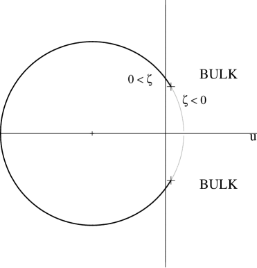
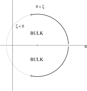
(a) Subcritical wall centered on $-u_{0}$.                  (b) Subcritical wall centered on $+u_{0}$.

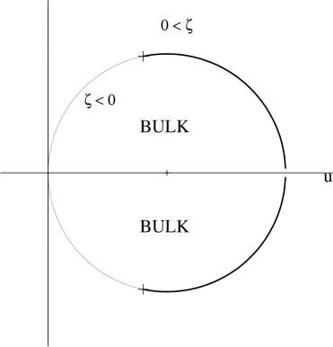
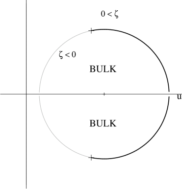
(c) Critical wall.                                            (d) Supercritical wall.

FIG. 1.: Wall trajectories given by equation 35, in euclidean signature. In each case the location of the bulk spacetime is indicated. In addition we have the simple critical wall trajectory given by $u=\text{const}$. Here the bulk lies to the right of the wall.

For subcritical walls, i.e., $\sigma_{n}<k_{n}$, $u_{0}<u_{1}$, and both branches of the hyperboloid (35) are allowed, which both intersect the adS boundary – see figure 1(a,b). An analysis of the normals to the braneworld shows that for a positive tension $Z_{2}$-symmetric braneworld, the upper root $Z^{\prime}>0$ corresponds to keeping the interior of the hyperboloid, whereas for $Z^{\prime}<0$ the exterior is kept. Supercritical walls on the other hand have only the upper root for $u_{0}$, and as $u_{0}>u_{1}$ in a euclidean signature they represent spheres which are entirely contained within the adS spacetime, the interior of the hyperboloid (or sphere) being kept for a positive tension braneworld (see figure 1(d)). For a critical wall, $\sigma_{n}=k_{n}$ there are once again two possible trajectories, one having the form of (35) but with $u_{0}=u_{1}=e^{k_{n}R_{0}}/2k_{n}$ (figure 1(c)), and the other having $u=$ const. – the RS braneworld.

To put a vortex on the braneworld, we require solutions with nonzero $\mu_{n}$, and hence a discontinuity in $Z^{\prime}$. To achieve this, we simply patch together different branches of the solutions (29) for $\zeta>0$ and $\zeta<0$. We immediately see that critical and supercritical walls can only support a vortex if $\kappa=1$, i.e., if the induced metric on the vortex itself is a de-Sitter universe. A subcritical wall on the other hand can support all induced geometries on the vortex. Defining $k_{n-1}^{2}=|a|$, these trajectories are

$$Z=\cases{{1\over 2k_{n-1}}\left[e^{\alpha-k_{n-1}|\zeta|}-\kappa e^{k_{n-1}|\zeta|-\alpha}\right]&subcritical wall\cr Z_{0}-|\zeta|&critical wall ($\kappa=1$)\cr{1\over k_{n-1}}\cos\left(k_{n-1}|\zeta|+\beta\right)&supercritical wall ($\kappa=1$)\cr}$$ (37)

where

$$\mu_{n}=\cases{{4k_{n-1}\over\sigma_{n}}\left[{e^{2\alpha}+\kappa\over e^{2\alpha}-\kappa}\right]&$\kappa=\pm 1,0$ subcritical wall\cr{4\over k_{n}Z_{0}}&critical wall\cr{4k_{n-1}\over\sigma_{n}}\tan\beta&supercritical wall\cr}$$ (38)

respectively.

A particularly useful example, for the purposes of illustrating the geometry of the ribbon, is to consider a vacuum bulk spacetime, which will obviously represent a supercritical braneworld. This removes any question of the warping of the bulk due to the cosmological constant, and shows particularly clearly the similarities and differences between the ribbon spacetime, an isolated vortex, and a domain wall in $(n-1)$-dimensional de-Sitter spacetime (the supercritical braneworld).

The case where there is no bulk cosmological constant has $k_{n}=0$, hence $k_{n-1}=\sigma_{n}$, and a pure domain wall universe would be a hyperboloid [37] – an accelerating bubble of proper radius $\sigma_{n}^{-1}$ in Minkowski spacetime, for which $\kappa=1$. For future comparison, we also note that a pure $\delta$-function vortex solution in a vacuum spacetime has a conical deficit metric

$$ds^{2}=dt^{2}-d{\bf x}^{2}-d\rho^{2}-\left(1-{\Delta\theta\over 2\pi}\right)^{2}\rho^{2}d\theta^{2}$$ (39)

where $\Delta\theta\simeq\mu_{n}$ for small $\mu_{n}$[38].

Reading off the domain ribbon trajectory from (37) gives in $(R,Z)$ space

$$Z = {1\over\sigma_{n}\sqrt{16+\mu_{n}^{2}}}\left[4\cos(\sigma_{n}\zeta)-\mu_{n}\sin(\sigma_{n}|\zeta|)\right]$$ (41)

$$R = {1\over\sigma_{n}\sqrt{16+\mu_{n}^{2}}}\left[4\sin(\sigma_{n}\zeta)\pm\mu_{n}[\cos(\sigma_{n}\zeta)-1]\right]$$ (42)

preserving the region $Z<Z(\zeta)$ of the bulk:

$$ds^{2}=Z^{2}\left[dt^{2}-\cosh^{2}\!t\ d\Omega_{n-3}^{2}\right]-dZ^{2}-dR^{2}$$ (43)

This is of course simply a coordinate transformation of Minkowski spacetime, with the appropriate limit of (31) being $({\tilde{t}},{\tilde{\bf x}})=(Z\sinh t,Z{\bf n}\cosh t)$. Transforming into Minkowski coordinates therefore, we find that the vacuum braneworld domain ribbon is given by two copies of the interior of the sliced hyperboloid

$${\tilde{\bf x}}^{2}-{\tilde{t}}^{2}+\left(|R|+{\mu_{n}\over\sigma_{n}\sqrt{16+\mu_{n}^{2}}}\right)^{2}={1\over\sigma_{n}^{2}}$$ (44)

If $\mu_{n}=0$ this is clearly the standard domain wall hyperboloid, however, for $\mu_{n}>0$ this now represents a hyperboloid which has had a slice of width $2\mu_{n}/\sigma_{n}\sqrt{16+\mu_{n}^{2}}$ removed from it (see figure 2).

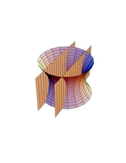
FIG. 2.: Constructing a domain ribbon on a vacuum domain wall. The hyperboloid interior has a slice of thickness $2\mu_{n}/\sigma_{n}\sqrt{16+\mu_{n}^{2}}$ removed from it, and is re-identified. The full spacetime consists of a second copy identified across the hyperboloid.

This corresponds rather well with the intuitive notion that walls are obtained by slicing and gluing spacetimes, and looking at a constant time slice (figure 3) we also see how the domain ribbon

FIG. 3.: Taking a constant time slice through the vacuum domain wall plus vortex spacetime shows how the deficit angle is built up.

looks like a vortex, with the identifications giving rise to a conical deficit angle in terms of the overall $n$-dimensional spacetime. A crucial difference here however appears to be that we can have an arbitrarily large energy per unit length of this vortex, as we simply cut out more and more of the hyperboloid. In terms of the conical deficit, we find

$$\Delta\theta=4\tan^{-1}\mu_{n}/4$$ (45)

and therefore the deficit angle approaches $2\pi$ only as $\mu_{n}$ approaches infinity! Contrast this with the spacetime of a pure vortex, (39), in which the deficit angle approaches $2\pi$ as $\mu_{n}\simeq 1$ [39], clearly the ribbon is not behaving as a vortex for large $\mu$. On the other hand, a domain wall has the effect of compactifying its spatial sections (the interior of the hyperboloid) and the transverse dimension only shrinks to zero size as the tension of the wall becomes infinite. Therefore in this sense, the ribbon spacetime really does behave as a domain wall.

We can also write down the induced metric on the domain wall brane-universe:

$$ds_{n-1}^{2}={[4\cos\sigma_{n}\zeta-\mu_{n}\sin\sigma_{n}|\zeta|]^{2}\over\sigma_{n}^{2}(16+\mu_{n}^{2})}\left[dt^{2}-\cosh^{2}td\Omega^{2}_{n-3}\right]-d\zeta^{2}$$ (46)

which is the metric of an $(n-2)$-dimensional domain wall in an $(n-1)$-dimensional de-Sitter universe of tension

$$G_{n-1}T={(n-3)\sigma_{n}G_{n}\over 2}\mu$$ (47)

i.e., with the identification (28) (using $\sigma_{n}$, rather than $k_{n}$ which is of course zero in this case) $T\equiv\mu$.

Having constructed this symmetric vacuum domain ribbon spacetime, we now see the general principle involved in having a domain ribbon. Whereas the braneworld consists of two segments of adS (or vacuum/dS) spacetime glued across a boundary, the domain ribbon consists of two copies of an adS spacetime with a kinked boundary (which could itself be viewed as two copies of an adS bulk glued together across a tensionless boundary making a kink) identified together. Therefore a domain ribbon on a critical wall in conformal coordinates is obviously the critical hyperboloid sliced by a critical flat RS wall (see figure 4).

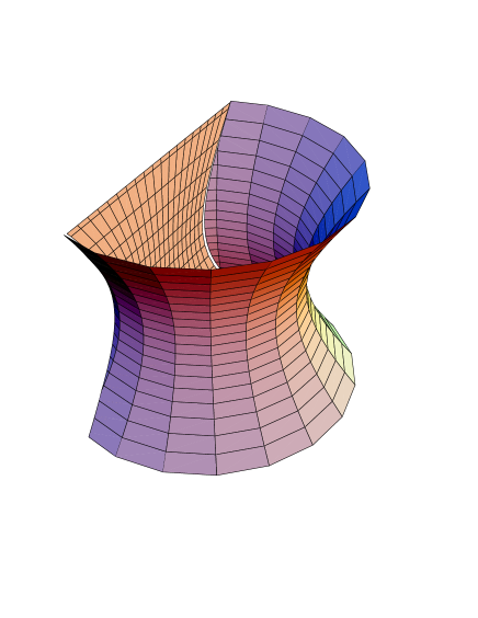
FIG. 4.: A representation of the domain ribbon in a critical RS universe.

Once more, as $\mu$ increases, more and more of the hyperboloid is removed, with the spacetime ‘disappearing’ only as $\mu\to\infty$.

We can also construct a range of nested Randall-Sundrum type configurations, i.e., flat ribbon geometries on adS braneworld trajectories within the bulk adS spacetime. From (30) we see that a flat ribbon geometry requires a subcritical wall, which in conformal coordinates has the form

$${\tilde{x}}^{1}=\pm{\sigma_{n}\over k_{n-1}}(u-u_{0})$$ (48)

For example, the original RSI domain ribbon would have the form (taking the universal covering) of a sawtooth trajectory:

$$R=2j(u_{1}-u_{0}){\sigma_{n}\over k_{n-1}}\pm{\sigma_{n}\over k_{n-1}}(u-u_{0})\;\;\;j\in Z$$ (49)

with alternate positive and negative tension ribbons. Similarly, one can construct a nested GRS scenario [40] :

$$u=\cases{u_{0}-{k_{n-1}|R|\over\sigma_{n}}&$|R|<{\sigma_{n}\over k_{n-1}}(u_{1}-u_{0})$\cr u_{1}&otherwise\cr}$$ (50)

although whether this displays a quasilocal graviton is not so easy to determine.

In principle one can construct all sorts of nested multibrane scenarios, however one suspects that the more baroque the model, the less stable or useful it is likely to be.

IV Instantons and tunneling on the brane

Traditionally, instantons correspond to classical euclidean solutions to the equations of motion. In many cases, they represent a quantum tunneling from a metastable false vacuum to a true vacuum. In  [31], Coleman and de Luccia discussed the effect of gravity on these decays. Such processes, of course have direct relevance for cosmology, as they correspond to a first order phase transition, and hence a dramatic change in the structure of our universe.

In  [31], the authors evaluated the probability of nucleation of a true vacuum bubble in a false vacuum background. They focussed on two particular configurations: a flat bubble spacetime in a de Sitter false vacuum; and an adS bubble spacetime in a flat false vacuum. This was before the idea of large extra dimensions was fashionable, so the analysis was done in just the usual four dimensions.

We now have the tools to develop these ideas in a brane world set up. To replicate the configurations of  [31], we just have to patch together our wall trajectories in the right way. Recall that these trajectories are given by equation (35), along with the critical wall solution, $u=\text{const}$. In euclidean signature, the former are shaped like spheres and were illustrated in figure 1. However, when patching these solutions together, we should be aware of a slight subtlety. In equation (25), the $\mu_{n}\sigma_{n}\delta(\zeta)$ term does not make sense if we have walls of different type either side of the vortex. Suppose we have a wall of tension $\sigma_{n}^{+}$ in $\zeta>0$, and $\sigma_{n}^{-}$ in $\zeta<0$, we must then modify equation (25) by replacing $\sigma_{n}$ with $\bar{\sigma}_{n}$, where

$$\bar{\sigma}_{n}={\sigma_{n}^{+}+\sigma_{n}^{-}\over 2}$$ (51)

It is easy to see that this is the right thing to do. Regard the vortex as a thin wall limit of some even energy distribution. Mathematically, this corresponds to $\mu_{n}\delta(\zeta)$ being the limit of some even function $\mu_{n}f(\zeta)$. The weight of the distribution is the same on either side of $\zeta=0$, so we pick up the average of the wall tensions.

We are now in a position to reproduce the work of  [31] in our higher dimensional environment. Let us consider first the decay of a de Sitter false vacuum, and the nucleation of a flat bubble spacetime.

A Nucleation of a flat bubble spacetime in a de Sitter false vacuum

We now describe the brane world analogue of the nucleation of a flat bubble spacetime in a de Sitter false vacuum. The de Sitter false vacuum is given by a supercritical wall of tension $\sigma_{n}^{dS}>k_{n}$ with no vortex (see figure 1(d)). This metastable state decays into a “bounce” configuration given by a critical wall (tension $\sigma_{n}^{flat}=k_{n}$) patched on to a supercritical wall (tension $\sigma_{n}^{dS}>k_{n}$). If we are to avoid generating an unphysical negative tension vortex we must patch together trajectories in the following way:

$$Z=\cases{{1\over k_{n-1}^{dS}}\cos(k_{n-1}^{dS}\zeta-\zeta_{0})&$\zeta>0$\cr\zeta+{1\over k_{n-1}^{dS}}\cos\zeta_{0}&$\zeta<0$\cr}$$ (52)

where $(k_{n-1}^{dS})^{2}=(\sigma_{n}^{dS})^{2}-k_{n}^{2}$. The vortex tension $\mu$, is related to the constant $\zeta_{0}$ in the following way:

$${\mu_{n}\bar{\sigma}_{n}\over 2k_{n-1}^{dS}}=\sec\zeta_{0}-\tan\zeta_{0}$$ (53)

It is useful to have a geometrical picture of this bounce solution. We just patch together the $u=$ const. critical wall trajectory and the supercritical wall trajectory given by figure 1(d) to get figure 5. Note that we have two copies of the bulk spacetime because we imposed $Z_{2}$-symmetry across the walls.

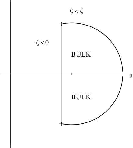
FIG. 5.: An example of a critical-supercritical wall “bounce” solution. This looks like a flat bubble spacetime has nucleated on a de Sitter wall.

It is natural to calculate the probability, $\mathcal{P}$, that this flat bubble spacetime does indeed nucleate on the de Sitter wall.

$${\mathcal{P}}\propto e^{-B}$$ (54)

where $B$ is the difference between the euclidean actions of the bounce solution and the false vacuum solution, that is:

$$B=S_{bounce}-S_{false}$$ (55)

Given our geometrical picture it is straightforward to write down an expression for the bounce action:

$$S_{bounce}=S_{bulk}+S_{flat}+S_{dS}+S_{vortex}$$ (56)

where the contribution from the bulk, critical wall (flat), supercritical wall (de Sitter), and vortex are as follows

$$S_{bulk} = -\frac{1}{16\pi G_{n}}\int_{bulk}d^{n}x\sqrt{g}(R-2\Lambda)$$ (58)

$$S_{flat} = -\frac{1}{16\pi G_{n}}\int_{flat}d^{n-1}x\sqrt{h}(-2\Delta K-4(n-2)\sigma_{n}^{flat})$$ (59)

$$S_{dS} = -\frac{1}{16\pi G_{n}}\int_{dS}d^{n-1}x\sqrt{h}(-2\Delta K-4(n-2)\sigma_{n}^{dS})$$ (60)

$$S_{vortex} = \mu\int_{vortex}d^{n-2}x\sqrt{\gamma}=-\frac{1}{16\pi G_{n}}\int_{vortex}d^{n-2}x\sqrt{\gamma}(-2\mu_{n})$$ (61)

Note that $\Delta K$, the jump in the trace of the extrinsic curvature across the wall, contains the Gibbons-Hawking boundary term [41] for each side of the wall, and $h_{ab}$, $\gamma_{\mu\nu}$ are the induced metrics on the wall and vortex respectively. We should point out that due to the presence of the vortex, there is a delta function in the extrinsic curvature that exactly cancels off the contribution of $S_{vortex}$. The expression for $S_{false}$ is similar except that there is no flat wall or vortex contribution, and no delta function in the extrinsic curvature. After some calculation (see Appendix), we find that our probability term, $B$ is given by:

$$B={4k_{n}^{2-n}\Omega_{n-2}\over 16\pi G_{n}}\left(I_{n}-\left({1\over n-1}\right)\left({k_{n}\cos\zeta_{0}\over k_{n-1}^{dS}}\right)^{n-1}\right)$$ (62)

where $\Omega_{n-2}$ is the volume of an $(n-2)$ sphere and the integral $I_{n}$ is given by:

$$I_{n}=\int_{u_{0}-u_{1}}^{u_{c}}du\quad\left(u_{0}{[\rho(u)]^{n-3}\over u^{n-1}}-{[\rho(u)]^{n-1}\over u^{n}}\right)$$ (63)

where

$$u_{0} = {\sigma_{n}^{dS}\over(k_{n-1}^{dS})^{2}}(\sigma_{n}^{dS}+k_{n}\sin\zeta_{0})u_{c}$$ (65)

$$u_{1} = {k_{n}\over\sigma_{n}^{dS}}u_{0}$$ (66)

$$\rho(u) = \sqrt{u_{1}^{2}-(u-u_{0})^{2}}$$ (67)

Note that $u_{c}$ is an arbitrary constant so we are free to choose it as we please (think of the flat wall as being at $u=u_{c}$). This integral is non trivial and although we can in principle solve it for any integer $n$ it would not be instructive to do so. Instead, we will restrict our attention to the case where $n=5$. This means that our braneworld is four dimensional, so comparisons with  [31] are more natural. Given that $\Omega_{3}=2\pi^{2}$, we find that:

$$B={8\pi^{2}k_{5}^{-3}\over 16\pi G_{5}}\Biggl{[}\log\left[{\sigma_{5}^{dS}+k_{5}\sin\zeta_{0}\over\sigma_{5}^{dS}+k_{5}}\right]-{1\over 2}\left({k_{5}\cos\zeta_{0}\over k_{4}^{dS}}\right)^{2}+{k_{5}\sigma_{5}^{dS}\over(k_{4}^{dS})^{2}}\left(1-\sin\zeta_{0}\right)\Biggr{]}$$ (68)

Equation (53) in five dimensions enables us to replace the trigonometric functions using:

$$\cos\zeta_{0} = {2\lambda\over 1+\lambda^{2}}$$ (70)

$$\sin\zeta_{0} = {1-\lambda^{2}\over 1+\lambda^{2}}$$ (71)

where

$$\lambda={\mu_{5}\bar{\sigma}_{5}\over 2k_{4}^{dS}}$$ (72)

This leads to a complicated expression. It is perhaps more instructive to examine the behaviour for small $\mu$ i.e., in the regime where we have a vortex with a low energy density. In this regime we find that:

$$B={256\pi^{5}\over(k^{dS}_{4})^{6}}(G_{5}\bar{\sigma}_{5})^{3}\mu^{4}+\mathcal{O}\rm(\mu^{5})={256\pi^{5}\over(k^{dS}_{4})^{6}}(\bar{G}_{4})^{3}\mu^{4}+\mathcal{O}\rm(\mu^{5})$$ (73)

where $\bar{G}_{4}$ is the average of the four dimensional Newton’s constants on the flat wall and the de Sitter wall. The presence of this average as opposed to a single four dimensional Newton’s constant is due to the difference in brane tension on either side of the vortex. From equation (28) we see that this induces a difference in the Newton’s constants on each wall.

We now compare this to the result we would have got had we assumed no extra dimensions. The analogous probability term, $B^{\prime}$, is calculated in  [31]. When the energy density of the bubble wall, $\mu$, is small, we now find that:

$$B^{\prime}={256\pi^{5}\over(k_{4})^{6}}(G_{4})^{3}\mu^{4}+\mathcal{O}\rm(\mu^{5})$$ (74)

If we associate $G_{4}$ in equation (74) with $\bar{G}_{4}$ in equation (73) we see that the approach of  [31], where no extra dimensions are present, yields exactly the same result to the braneworld setup, at least for small $\mu$.

Before we move on to discuss alternative instanton solutions we should note that in the above analysis we have assumed ${\pi\over 2}>\zeta_{0}>0$. The bounce solution presented is therefore really only valid if we have $\lambda<1$. However, the extension to regions where $\lambda>1$ corresponds to allowing $\zeta_{0}$ to take negative values and everything holds.

B Nucleation of an adS bubble spacetime in a flat false vacuum

We now turn our attention to the decay of a flat false vacuum, and the nucleation of an adS bubble spacetime. The braneworld analogue of the flat false vacuum is given by a critical wall of tension $\sigma_{n}^{flat}=k_{n}$ with no vortex ($u=$ const). This decays into a new “bounce” configuration given by a subcritical wall (tension $\sigma_{n}^{adS}<k_{n}$) patched onto a critical wall (tension $\sigma_{n}^{flat}=k_{n}$). Again, in order to avoid generating an unphysical vortex, we must patch together trajectories in the following way:

$$Z=\cases{\zeta+{1\over k_{n-1}^{adS}}\sinh\zeta_{0}&$\zeta>0$\cr{1\over k_{n-1}^{adS}}\sinh(k_{n-1}^{adS}\zeta+\zeta_{0})&$\zeta<0$}$$ (75)

where $(k_{n-1}^{adS})^{2}=k_{n}^{2}-(\sigma_{n}^{adS})^{2}$. The vortex tension $\mu$ is related to the constant $\zeta_{0}$ in the following way:

$${\mu_{n}\bar{\sigma}_{n}\over 2k_{n-1}^{adS}}=\textrm{coth}\zeta_{0}-\textrm{cosech}\zeta_{0}$$ (76)

By patching together $u=$ const. and figure 1(a) we again obtain a geometrical picture of our bounce solution (see figure 6).

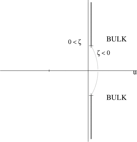
FIG. 6.: An example of a subcritical-critical wall “bounce” solution. This looks like an adS bubble spacetime has nucleated on a flat wall.

As before we now consider the probability term, $B$, given by the difference between the euclidean actions of the bounce and the false vacuum. We shall not go into great detail here as the calculation is very similar to that in the previous section. We should emphasize, however, that the bounce action will include as before an Einstein-Hilbert action with negative cosmological constant in the bulk, a Gibbons Hawking surface term on each wall, and tension contributions from each wall and the vortex. Again we find that the delta function in the extrinsic curvature of the brane exactly cancels off the contribution from the vortex tension. The false vacuum action omits the adS wall and vortex contributions, and contains no delta functions from extrinsic curvature. Recall that in each case we have two copies of the bulk spacetime because of $Z_{2}$-symmetry across the wall.

This time, we find that our probability term, $B$, is given by:

$$B={4k_{n}^{2-n}\Omega_{n-2}\over 16\pi G_{n}}\left(I_{n}+\left({1\over n-1}\right)\left({k_{n}\sinh\zeta_{0}\over k_{n-1}^{adS}}\right)^{n-1}\right)$$ (77)

where the integral $I_{n}$ is now given by:

$$I_{n}=\int_{-u_{0}+u_{1}}^{u_{c}}du\quad\left(u_{0}{[\rho(u)]^{n-3}\over u^{n-1}}+{[\rho(u)]^{n-1}\over u^{n}}\right)$$ (78)

where $u_{c}$ is an arbitrary constant corresponding to the position of the flat wall, and

$$u_{0} = {\sigma_{n}^{adS}\over(k_{n-1}^{adS})^{2}}(\sigma_{n}^{dS}+k_{n}\cosh\zeta_{0})u_{c}$$ (79)

$$u_{1} = {k_{n}\over\sigma_{n}^{adS}}u_{0}$$ (80)

$$\rho(u) = \sqrt{u_{1}^{2}-(u+u_{0})^{2}}$$ (81)

Again, although we could in principle solve this integral for any positive integer $n$, we shall restrict our attention to $n=5$. In this case we now find that:

$$B={8\pi^{2}k_{5}^{-3}\over 16\pi G_{5}}\Biggl{[}-\log\left[{\sigma_{5}^{adS}+k_{5}\cosh\zeta_{0}\over\sigma_{5}^{adS}+k_{5}}\right]+{1\over 2}\left({k_{5}\sinh\zeta_{0}\over k_{4}^{adS}}\right)^{2}+{k_{5}\sigma_{5}^{adS}\over(k_{4}^{adS})^{2}}\left(1-\cosh\zeta_{0}\right)\Biggr{]}$$ (82)

We can now replace the hyperbolic functions using equation (76):

$$\sinh\zeta_{0} = {2\lambda\over 1-\lambda^{2}}$$ (84)

$$\cosh\zeta_{0} = {1+\lambda^{2}\over 1-\lambda^{2}}$$ (85)

where

$$\lambda={\mu_{5}\bar{\sigma}_{5}\over 2k_{4}^{adS}}$$ (86)

This is again an ugly expression. It is more interesting to examine the behaviour at small $\mu$:

$$B={256\pi^{5}\over(k^{adS}_{4})^{6}}(G_{5}\bar{\sigma}_{5})^{3}\mu^{4}+\mathcal{O}\rm(\mu^{5})={256\pi^{5}\over(k^{adS}_{4})^{6}}(\bar{G}_{4})^{3}\mu^{4}+\mathcal{O}\rm(\mu^{5})$$ (87)

This is very similar to what we had for the nucleation of a flat bubble spacetime in a de Sitter false vacuum with $\bar{G}_{4}$ now representing the average of the Newton’s constants on the adS wall and the flat wall. Again we compare this to the result from  [31] where we have no extra dimensions. When the energy density of the bubble wall is small, the expression for the probability term is again given by equation (74), where ${1\over k_{4}}$ now corresponds to the radius of curvature of the adS spacetime. Once again we see that the braneworld result agrees exactly with  [31] in the small $\mu$ limit, provided we associate $G_{4}$ with $\bar{G}_{4}$.

Note that again we have assumed $\zeta_{0}>0$ and therefore, the bounce solution given here is only valid for $\lambda<1$. The extension to $\lambda>1$ is more complicated than for the nucleation of the flat bubble in the previous section. We now have to patch together figure 1(b) and figure 1(c). However, in  [31], the analogue of $\lambda>1$ violates conservation of energy as one tunnels from the false vacuum to the new configuration. In the braneworld set up we should examine what happens as $\lambda$ approaches unity from below. In this limit, $\zeta_{0}$ becomes infinite, and the adS bubble encompasses the entire brane. The probability, $\mathcal{P}$, of this happening is zero and so there is no vacuum decay. Beyond this, in analogy with  [31], we would suspect that the energy of the false vacuum is insufficient to allow the nucleation of a bubble with a large wall energy density. This is indeed the case. When we calculate the probability term, $B$, for the adS bubble in a flat, spherical false vacuum, we find that it is divergent and the probability of bubble nucleation vanishes. This divergence comes from the fact that the false vacuum touches the adS boundary whereas the bounce solution does not.

Finally, we could also have created an adS bubble in a flat spacetime using a $\kappa=0$ vortex. However, it is of no interest since the probability of bubble nucleation is exponentially suppressed by the vortex volume.

C Ekpyrotic Instantons

The notion of the Ekpyrotic universe [32] proposes that the Hot Big Bang came about as the result of a collision between two braneworlds. The model claims to solve many of the problems facing cosmology without the need for inflation. Although the authors work mainly in the context of heterotic M theory, they acknowledge that an intuitive understanding can be gained by considering Randall-Sundrum type braneworlds. In this context, we regard the pre-Big Bang era in the following way. We start off with two branes of equal and opposite tension: the hidden brane of positive tension, $\sigma$, and the visible brane of negative tension, $-\sigma$. A bulk brane with a small positive tension, ${\epsilon\over 2}$, then “peels off” the hidden brane causing its tension to fall to $\sigma-\epsilon$. The bulk brane is then drawn towards our universe, the visible brane, until it collides with us, giving rise to the Hot Big Bang.

The process of “peeling off” is not really considered in great detail in  [32]. They suggest that the hidden brane undergoes a small instanton transition with the nucleation of a bubble containing a new hidden brane with decreased tension, and the bulk brane. The walls of this bubble then expand at the speed of light until it envelopes all of the old hidden brane. Given that all the branes in this model are critical we can illustrate the instanton solution in the simplified RS set-up by using a suitable combination of critical wall solutions. In conformal coordinates, critical walls look like planes ($u=\text{const}$) or spheres (see figure 1(c)). In describing the Ekpyrotic instanton we present the visible and hidden branes (old and new) as planes. The bulk brane is given by a sphere that intersects the hidden brane, separating the old and new branches (see figure 7).

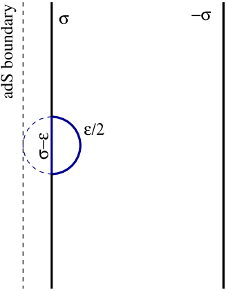
FIG. 7.: The Ekpyrotic Instanton

Given this geometrical picture we can calculate the probability of tunneling to this configuration from the initial two brane state. We proceed much as we did in the previous section, and obtain the following expression for the probability term:

$$B={\pi^{2}\epsilon\over 4}\left({3\over k^{3}}\ln(1+k^{2}Z_{0}^{2})-{2k^{-2}Z_{0}^{2}\over 1+k^{2}Z_{0}^{2}}-{Z_{0}^{2}\over k^{2}}-{Z_{0}^{4}\over 4}\right)+\mathcal{O}\rm(\epsilon^{2})$$ (88)

where $k$ is related to the cosmological constant in the bulk of the initial state ($\Lambda=-6k^{2}$), and $Z_{0}$ is a free parameter related to the “size” of the bubble: the larger the value of $Z_{0}$, the larger the bubble. We should not be worried by this freedom in $Z_{0}$, as we are working with Randall-Sundrum braneworlds which are much simpler than the M5 branes of heterotic M theory. When we return to the M theory context, we lose a number of degrees of freedom and one might expect the value of $Z_{0}$ to be fixed. However, since we are dealing with a “small’ instanton, we might expect $Z_{0}$ itself to be small, and the probability term approximates to the following:

$$B={\pi^{2}\over 16}\epsilon Z_{0}^{4}+\mathcal{O}\rm(\epsilon^{2},Z_{0}^{6})$$ (89)

We should once again stress however, that this is an extremely simple and naive calculation that ignores any dynamics of the additional scalars, or other fields, that result from a five-dimensional heterotic M-theory compactification [42]. Another point to note is that while we can have a small brane peel off from the positive tension braneworld, we cannot have one peel off from the negative tension braneworld, as a quick glance at figure 7 shows. Such a brane, being critical, must have the form of a sphere grazing the adS boundary, which therefore necessarily would intersect the positive tension brane as well.

V Discussion

In this paper we have derived the general spacetime of an infinitesimally thin braneworld containing a nested domain wall or domain ribbon. These results can be regarded as a “zero-thickness” limit of some thick braneworld (and ribbon) field theory model, in much the same way as the Randall-Sundrum model can be regarded as the limit of a thick brane. The ribbon can therefore be interpreted as a kink in a scalar condensate living on the brane. Cosmologically, this scalar plays the role of an inflaton, which can therefore potentially give rise to an old inflationary model. In section IV we determined the instanton for false vacuum decay, however, we found that the presence of the extra dimension does not ameliorate the usual problems afflicting old inflation.

Given that these results were obtained in the absence of the adS soliton c-term, a natural question might be to ask how they are modified for $c\neq 0$, in the canonical metric (10). The adS soliton was originally investigated by Horowitz and Myers [34] in the context of a modified positive energy conjecture in asymptotically locally adS spacetimes, and has also been used to obtain braneworld solutions in six dimensions [43, 44]. These models slice the flat ($\kappa=0$) soliton cigar in six dimensions at fixed ‘radius’ – which corresponds to a source consisting of a superposition of a 4-brane and a smeared 3-brane (i.e., smearing out our $\delta$-function source throughout the 4-brane). In addition these papers also included 3-branes located at the euclidean horizon $Z_{+}$, via conical deficits in the $R$-coordinate.

Clearly we can use our formalism to re-localize the 3-brane of [43, 44], as well as derive more general braneworlds with arbitrary $\kappa$, tension $\sigma$, and overall spacetime dimension $n$. Leaving a detailed study for later work, we now simply remark on the qualitative behaviour of such braneworlds. The equations of motion (II) for a $Z_{2}$-symmetric trajectory become:

$$Z^{\prime 2} = aZ^{2}+\kappa-{c\over Z^{n-3}}$$ (91)

$$Z^{\prime\prime} = aZ+\left({n-3\over 2}\right){c\over Z^{n-2}}-4\pi G_{n}\sum_{i}\mu_{i}\sigma_{n}Z\delta(\zeta-\zeta_{i})$$ (92)

$$R^{\prime} = {\sigma_{n}Z^{n-2}\over k_{n}^{2}Z^{n-1}+\kappa Z^{n-3}-c}$$ (93)

where $a=k_{n}^{2}-\sigma_{n}^{2}$ as before, and (92) now allows for a multitude of domain ribbons of tension $\mu_{i}$ located at $\zeta_{i}$.

We can quickly see the qualitative behaviour of solutions to these equations. The generic trajectory (which must be periodic in $R$) will consist of two segments of $Z(\zeta)$ of opposite gradient which patch together at a positive tension domain ribbon at $R=0$, say, and a negative tension domain ribbon at $R=\Delta R/2$. This is exactly analogous to the usual situation with a domain wall spacetime when we need both positive and negative tension walls to form a compact extra dimension. However, we see that with the bulk “mass” term, there are now also other possibilities, since (91) now has at least one root for $Z>Z_{+}$, and in fact two for supercritical walls. This root corresponds to a zero of $Z^{\prime}$, and hence the possibility for a smooth transition from the positive branch of $Z^{\prime}$ to the negative branch. We can therefore form a trajectory which loops symmetrically around the cigar, and has only one kink – which we can fix to be a positive tension vortex. Of course, the tension of this vortex will be determined by the other parameters of the set-up: the bulk mass, cosmological constant and the braneworld tension, but this is no worse a fine tuning than is already present in conventional RS models. Note that this is now distinct from a domain wall on a compact extra dimension, as we can construct a domain ribbon spacetime with only a single positive tension ribbon on all braneworld geometries i.e., with positive (supercritical), zero (critical) or negative (subcritical) induced cosmological constants. In addition, for a supercritical braneworld (i.e., a positive induced cosmological constant) we have the possibility of dispensing with the ribbon altogether, and having a smooth trajectory with two roots of $Z^{\prime}$, where the braneworld smoothly wraps the cigar, although this requires a fine tuned mass term.

In all cases the induced braneworld geometry has the form

$$ds^{2}=Z^{2}(\zeta)\left[dX_{n-2}^{2}\right]_{\kappa}-d\zeta^{2}$$ (94)

(where of course $\zeta$ has a finite range). The energy momentum tensor of this spacetime is

$$8\pi G_{n-1}T^{\mu}_{\nu} = \left[-(n-3){Z^{\prime\prime}\over Z}-{(n-3)(n-4)\over 2}{(Z^{\prime 2}-\kappa)\over Z^{2}}+{(n-3)\over 2}\mu_{n}\sigma_{n}\delta(\zeta)\right]\delta^{\mu}_{\nu}$$ (96)

$$= -{(n-3)\over 2}\left[(n-2)a+{c\over Z^{n-1}}-\mu_{n}\sigma_{n}\delta(\zeta)\right]\delta^{\mu}_{\nu}$$ (97)

$$8\pi G_{n-1}T^{\zeta}_{\zeta} = -{(n-2)(n-3)\over 2}{(Z^{\prime 2}-\kappa)\over Z^{2}}=-{(n-2)(n-3)\over 2}\left(a-{c\over Z^{n-1}}\right)$$ (98)

which has three distinct components: A cosmological constant (the $a$-term) which reflects the lack of criticality of the braneworld when it is nonvanishing. The domain ribbon terms ($\mu_{i}$) when present indicate the presence of a nested $(n-3)$-brane – note the normalization is precisely correct for the induced $(n-1)$-dimensional Newton’s constant. And the final $c$-term is in fact a negative stress-energy tensor, which is of Casimir form, and can be directly associated to the Casimir energy of the CFT living in the braneworld, in the same way as the stress-tensor of the radiation cosmology obtained by slicing a standard Schwarzschild-adS black hole can be interpreted as the energy of the CFT at finite Hawking temperature on the braneworld [24].

A Details of Instanton Calculation

In section IV we calculated the probability of bubble nucleation in a number of braneworld situations. The details of these calculations are remarkably similar for both the flat bubble and the AdS bubble. In this Appendix we shall present the calculation for the flat bubble spacetime forming in a de Sitter false vacuum.

Consider now equations (56a-d). Our solution satisfies the equations of motion both in the bulk and on the brane. The bulk equations of motion are just Einstein’s equations (in euclidean signature) with a negative cosmological constant:

$$R_{ab}-{1\over 2}Rg_{ab}=-\Lambda g_{ab}$$ (A1)

from which we can quickly obtain

$$R-2\Lambda={4\Lambda\over n-2}=-2(n-1)k_{n}^{2}$$ (A2)

where we have used the relation (12). The brane equations of motion are just the Israel equations given that we have a brane tension and a nested domain wall:

$$\Delta K_{\mu\nu}-\Delta Kh_{\mu\nu}=8\pi G_{n}\sigma h_{\mu\nu}+8\pi G_{n}\mu\delta(\zeta)\gamma_{\mu\nu}$$ (A3)

where $\sigma$ is $\sigma^{flat}$ and $\sigma^{dS}$ on the flat and de Sitter walls respectively. We can therefore read off the following expression:

$$\Delta K=-2(n-1)\sigma_{n}-\mu_{n}\delta(\zeta)$$ (A4)

where we have also used (18). We are now ready to calculate the action. Inserting (A2) and (A4) in (56), we immediately see that the contribution from the vortex is cancelled off by the delta function in the extrinsic curvature and we are left with

$$S_{bounce}={2(n-1)k_{n}^{2}\over 16\pi G_{n}}\int_{bulk}d^{n}x\sqrt{g}-{4\sigma_{n}^{flat}\over 16\pi G_{n}}\int_{flat}d^{n-1}x\sqrt{h}-{4\sigma_{n}^{dS}\over 16\pi G_{n}}\int_{dS}d^{n-1}x\sqrt{h}$$ (A5)

The expression for $S_{false}$ is similar except that there is of course no flat wall contribution and the limits for the bulk and de Sitter brane integrals run over the whole of the de Sitter sphere interior and surface respectively.

Working in euclidean conformal coordinates (i.e., the metric (31) rotated to euclidean signature) the bulk measure is simply

$$\sqrt{g}d^{n}x={\rho^{n-2}\over(k_{n}u)^{n}}du\,d\rho\,d\Omega_{n-2}$$ (A6)

where $d\Omega_{n-2}$ is the measure on a unit $n-2$ sphere. From (35) and (63), the de Sitter wall is given by

$$(u-u_{0})^{2}+\rho^{2}=u_{1}^{2}$$ (A7)

so the induced metric on this wall is given by:

$$ds^{2}_{n-1}={1\over k_{n}^{2}u^{2}}\left[\left({k_{n}u_{0}\over\sigma^{dS}_{n}\rho(u)}\right)^{2}du^{2}+\rho(u)^{2}d\Omega_{n-2}\right]$$ (A8)

where $\rho(u)$ is given in (67). As we did for the bulk, we can now read off the de Sitter wall measure:

$$\sqrt{h}d^{n-1}x=u_{1}{\rho(u)^{n-3}\over(k_{n}u)^{n-1}}\,du\,d\Omega_{n-2}\,.$$ (A9)

Now consider the flat wall. This is given by $u=u_{c}$ where $u_{c}$ is given by (65), and the measure can be easily seen to be

$$\sqrt{h}d^{n-1}x={\rho^{n-2}\over(k_{n}u_{c})^{n-1}}\,d\rho\,d\Omega_{n-2}.$$ (A10)

Now we are ready to evaluate the probability term $B=S_{bounce}-S_{false}$. Given each of the measures we have just calculated and taking care to get the limits of integration right for both the bounce action and the false vacuum action, we arrive at the following expression:

$$B = -{4(n-1)k_{n}^{2}\over 16\pi G_{n}}\Omega_{n-2}\int_{u_{0}-u_{1}}^{u_{c}}du\int_{0}^{\rho(u)}d\rho{\rho^{n-2}\over(k_{n}u)^{n}}$$ (A12)

$$-{4\sigma_{n}^{flat}\over 16\pi G_{n}}\Omega_{n-2}\int_{0}^{\rho(u_{c})}d\rho{\rho^{n-2}\over(k_{n}u_{c})^{n-1}}+{4\sigma_{n}^{dS}\over 16\pi G_{n}}\Omega_{n-2}\int_{u_{0}-u_{1}}^{u_{c}}duu_{1}{\rho(u)^{n-3}\over(k_{n}u)^{n-1}}$$

We should note that we have a factor of two in the bulk part of the above equation arising from the fact that we have two copies of the bulk spacetime. If we use the fact that:

$$\rho(u_{c})={k_{n}u_{c}\over k_{n-1}^{dS}}\cos\zeta_{0}$$ (A14)

along with $\sigma_{n}^{flat}=k_{n}$ and equation (66), we can simplify (A12) to arrive at equation (62).

REFERENCES

- [1] V. A. Rubakov and M. E. Shaposhnikov, Phys. Lett. B125, 136 (1983).
- [2] K. Akama, Lect. Notes Phys. 176, 267 (1982) [hep-th/0001113].
-
[3]
N. Arkani-Hamed, S. Dimopoulos and G. Dvali,
Phys. Lett. B429, 263 (1998)
[hep-ph/9803315].
N. Arkani-Hamed, S. Dimopoulos and G. Dvali, Phys. Rev. D 59, 086004 (1999) [hep-ph/9807344].
I. Antoniadis, N. Arkani-Hamed, S. Dimopoulos and G. Dvali, Phys. Lett. B 436, 257 (1998) [hep-ph/9804398]. - [4] L. Randall and R. Sundrum, Phys. Rev. Lett. 83, 3370 (1999) [hep-ph/9905221].
- [5] L. Randall and R. Sundrum, Phys. Rev. Lett. 83, 4690 (1999) [hep-th/9906064].
-
[6]
J. Polchinski,
“TASI lectures on D-branes,”
hep-th/9611050.
P. Horava and E. Witten, Nucl. Phys. B 460, 506 (1996) [hep-th/9510209].
A. Lukas, B. A. Ovrut, K. S. Stelle and D. Waldram, Phys. Rev. D59, 086001 (1999) [hep-th/9803235].
A. Lukas, B. A. Ovrut and D. Waldram, Phys. Rev. D 60, 086001 (1999) [hep-th/9806022]. -
[7]
M. Visser,
Phys. Lett. B 159, 22 (1985)
[hep-th/9910093].
E. J. Squires, Phys. Lett. B 167, 286 (1986). -
[8]
C. Charmousis, R. Emparan and R. Gregory,
JHEP 0105, 026 (2001)
[hep-th/0101198].
R. Sundrum, Phys. Rev. D59 (1999) 085010 [hep-ph/9807348]. -
[9]
A. Chodos and E. Poppitz,
Phys. Lett. B 471, 119 (1999)
[hep-th/9909199].
T. Gherghetta and M. Shaposhnikov, Phys. Rev. Lett. 85, 240 (2000) [hep-th/0004014]. -
[10]
A. G. Cohen and D. B. Kaplan,
Phys. Lett. B 470, 52 (1999)
[hep-th/9910132].
A. Chodos, E. Poppitz and D. Tsimpis, Class. Quant. Grav. 17, 3865 (2000) [hep-th/0006093].
T. Gherghetta, E. Roessl and M. Shaposhnikov, Phys. Lett. B 491, 353 (2000) [hep-th/0006251]. -
[11]
R. Gregory,
Phys. Rev. Lett. 84, 2564 (2000)
[hep-th/9911015].
I. Olasagasti and A. Vilenkin, Phys. Rev. D 62, 044014 (2000) [hep-th/0003300].
M. Giovannini, H. Meyer and M. Shaposhnikov, hep-th/0104118. -
[12]
J. Garriga and T. Tanaka,
Phys. Rev. Lett. 84, 2778 (2000)
[hep-th/9911055].
S. B. Giddings, E. Katz and L. Randall, JHEP0003, 023 (2000) [hep-th/0002091]. - [13] C. Charmousis, R. Gregory and V. A. Rubakov, Phys. Rev. D 62, 067505 (2000) [hep-th/9912160].
- [14] T. Chiba, Phys. Rev. D 62, 021502 (2000) [gr-qc/0001029].
- [15] A. Chamblin and G. W. Gibbons, Phys. Rev. Lett. 84, 1090 (2000) [hep-th/9909130].
- [16] A. Chamblin, S. W. Hawking and H. S. Reall, Phys. Rev. D61, 065007 (2000) [hep-th/9909205].
- [17] R. Gregory, Class. Quant. Grav. 17, L125 (2000) [hep-th/0004101].
-
[18]
R. Emparan, G. T. Horowitz and R. C. Myers,
JHEP0001, 007 (2000)
[hep-th/9911043].
R. Emparan, G. T. Horowitz and R. C. Myers, JHEP0001, 021 (2000) [hep-th/9912135].
R. Emparan, R. Gregory and C. Santos, Phys. Rev. D 63, 104022 (2001) [hep-th/0012100]. -
[19]
P. Binetruy, C. Deffayet and D. Langlois,
Nucl. Phys. B565, 269 (2000)
[hep-th/9905012].
P. Binetruy, C. Deffayet, U. Ellwanger and D. Langlois, Phys. Lett. B477, 285 (2000) [hep-th/9910219]. -
[20]
M. Gogberashvili,
Europhys. Lett. 49, 396 (2000)
[hep-ph/9812365].
N. Kaloper and A. Linde, Phys. Rev. D 59, 101303 (1999) [hep-th/9811141].
T. Nihei, Phys. Lett. B 465, 81 (1999) [hep-ph/9905487].
C. Csaki, M. Graesser, C. Kolda and J. Terning, Phys. Lett. B462, 34 (1999) [hep-ph/9906513].
J. M. Cline, C. Grojean and G. Servant, Phys. Rev. Lett. 83, 4245 (1999) [hep-ph/9906523].
D. J. Chung and K. Freese, Phys. Rev. D61, 023511 (2000) [hep-ph/9906542].
P. Kanti, I. I. Kogan, K. A. Olive and M. Pospelov, Phys. Lett. B468, 31 (1999) [hep-ph/9909481].
E. E. Flanagan, S. H. Tye and I. Wasserman, Phys. Rev. D 62, 044039 (2000) [hep-ph/9910498].
D. N. Vollick, Class. Quant. Grav. 18, 1 (2001) [hep-th/9911181]. -
[21]
H. A. Chamblin and H. S. Reall,
Nucl. Phys. B 562, 133 (1999)
[hep-th/9903225].
N. Kaloper, Phys. Rev. D60, 123506 (1999) [hep-th/9905210].
P. Kraus, JHEP9912, 011 (1999) [hep-th/9910149].
J. Khoury, P. J. Steinhardt and D. Waldram, Phys. Rev. D 63, 103505 (2001) [hep-th/0006069]. - [22] P. Bowcock, C. Charmousis and R. Gregory, Class. Quant. Grav. 17, 4745 (2000) [hep-th/0007177].
-
[23]
D. Ida,
JHEP0009, 014 (2000)
[gr-qc/9912002].
H. Stoica, S. H. Tye and I. Wasserman, Phys. Lett. B 482, 205 (2000) [hep-th/0004126]. A. Davis, S. C. Davis, W. B. Perkins and I. R. Vernon, Phys. Lett. B 504, 254 (2001) [hep-ph/0008132].
R. A. Battye, B. Carter, A. Mennim and J. Uzan, hep-th/0105091. -
[24]
S. S. Gubser,
Phys. Rev. D 63, 084017 (2001)
[hep-th/9912001].
E. Verlinde, “On the holographic principle in a radiation dominated universe,” hep-th/0008140.
I. Savonije and E. Verlinde, Phys. Lett. B 507, 305 (2001) [hep-th/0102042]. -
[25]
S. W. Hawking, T. Hertog and H. S. Reall,
Phys. Rev. D 62, 043501 (2000)
[hep-th/0003052].
L. Anchordoqui, C. Nunez and K. Olsen, JHEP 0010, 050 (2000) [hep-th/0007064].
A. Hebecker and J. March-Russell, “Randall-Sundrum II cosmology, AdS/CFT, and the bulk black hole,” hep-ph/0103214. -
[26]
A. Sen,
JHEP 9808, 012 (1998)
[hep-th/9805170].
A. Sen, “Non-BPS states and branes in string theory,” hep-th/9904207. -
[27]
J. R. Morris,
Int. J. Mod. Phys. A 13, 1115 (1998)
[hep-ph/9707519].
J. R. Morris, Phys. Rev. D 51, 697 (1995). -
[28]
D. Bazeia, R. F. Ribeiro and M. M. Santos,
Phys. Rev. D 54, 1852 (1996).
J. D. Edelstein, M. L. Trobo, F. A. Brito and D. Bazeia, Phys. Rev. D 57, 7561 (1998) [hep-th/9707016].
D. Bazeia, H. Boschi-Filho and F. A. Brito, JHEP 9904, 028 (1999) [hep-th/9811084]. - [29] R. Gregory and A. Padilla, “Nested braneworlds and strong brane gravity,” hep-th/0104262.
- [30] W. Israel, Nuovo Cim. B 44S10, 1 (1966) [Erratum-ibid. B 48, 463 (1966)].
- [31] S. Coleman and F. De Luccia, Phys. Rev. D 21, 3305 (1980).
- [32] J. Khoury, B. A. Ovrut, P. J. Steinhardt and N. Turok, “The ekpyrotic universe: Colliding branes and the origin of the hot big bang,” hep-th/0103239.
- [33] K. A. Bronnikov and V. N. Melnikov, Gen. Rel. Grav. 27, 465 (1995) [gr-qc/9403063].
- [34] G. T. Horowitz and R. C. Myers, Phys. Rev. D 59, 026005 (1999) [hep-th/9808079].
- [35] U. Gen and M. Sasaki, “Radion on the de Sitter brane,” gr-qc/0011078.
-
[36]
I. I. Kogan, S. Mouslopoulos and A. Papazoglou,
Phys. Lett. B 501, 140 (2001)
[hep-th/0011141].
A. Karch and L. Randall, Int. J. Mod. Phys. A 16, 780 (2001) [hep-th/0011156].
M. D. Schwartz, Phys. Lett. B 502, 223 (2001) [hep-th/0011177]. -
[37]
G. W. Gibbons,
Nucl. Phys. B 394, 3 (1993).
M. Cvetic, S. Griffies and H. H. Soleng, Phys. Rev. D 48, 2613 (1993) [gr-qc/9306005]. - [38] A. Vilenkin, Phys. Rev. D 23, 852 (1981).
- [39] P. Laguna and D. Garfinkle, Phys. Rev. D 40, 1011 (1989).
- [40] R. Gregory, V. A. Rubakov and S. M. Sibiryakov, Phys. Rev. Lett. 84, 5928 (2000) [hep-th/0002072].
- [41] G. W. Gibbons and S. W. Hawking, Phys. Rev. D 15, 2752 (1977).
- [42] A. Lukas, B. A. Ovrut, K. S. Stelle and D. Waldram, Nucl. Phys. B 552, 246 (1999) [hep-th/9806051].
-
[43]
J. Chen, M. A. Luty and E. Ponton,
JHEP 0009, 012 (2000)
[hep-th/0003067].
E. Ponton and E. Poppitz, JHEP 0102, 042 (2001) [hep-th/0012033]. -
[44]
F. Leblond, R. C. Myers and D. J. Winters,
“Consistency conditions for brane worlds in arbitrary dimensions,”
hep-th/0106140.
F. Leblond, R. C. Myers and D. J. Winters, “Brane world sum rules and the AdS soliton,” hep-th/0107034.