SISSA/54/2001/FM

Boundary Quantum Field Theories with
Infinite Resonance States

P. Mosconi^1,2, G. Mussardo^1,3 and V. Riva¹

¹International School for Advanced Studies, Trieste, Italy
²Istituto Nazionale di Fisica della Materia, Sezione di Trieste
³Istituto Nazionale di Fisica Nucleare, Sezione di Trieste

We extend a recent work by Mussardo and Penati on integrable quantum field theories with a single stable particle and an infinite number of unstable resonance states, including the presence of a boundary. The corresponding scattering and reflection amplitudes are expressed in terms of Jacobian elliptic functions, and generalize the ones of the massive thermal Ising model and of the Sinh-Gordon model. In the case of the generalized Ising model we explicitly study the ground state energy and the one–point function of the thermal operator in the short–distance limit, finding an oscillating behaviour related to the fact that the infinite series of boundary resonances does not decouple from the theory even at very short–distance scales. The analysis of the generalized Sinh-Gordon model with boundary reveals an interesting constraint on the analytic structure of the reflection amplitude. The roaming limit procedure which leads to the Ising model, in fact, can be consistently performed only if we admit that the nature of the bulk spectrum uniquely fixes the one of resonance states on the boundary.

1 Introduction

The study of resonances in relativistic models has provided important insights into the general problem of the dynamics of quantum field theories. Resonances are usually due to unstable bound states which therefore do not appear as asymptotic states. However, associated to them, there are mass scales which may induce interesting and unexpected phenomena. Al. Zamolodchikov, for instance, has shown in [1] that a single resonance state produces a remarkable pattern of roaming Renormalization Group trajectories, with the property that they pass by very closely all minimal unitary models of Conformal Field Theory, finally ending in the massive phase of the Ising model. The first model with an infinite number of resonance states is due to A. Zamolodchikov, in relation with a QFT characterized by a dynamical $Z_{4}$ symmetry [2] (see also [3]). A simpler class of models with infinitely many resonance states have been considered by Mussardo and Penati in [4]. The analysis performed in [4] of the Form Factors and the correlation functions of these theories has shown a rather rich and still unexplored behaviour of such theories. A further step in the analysis of infinite resonance models has been taken by Castro–Alvaredo and Fring in [5].

The aim of this paper is to extend the analysis of the physical effects induced by an infinite tower of resonance states, this time also placed at the boundary of a $1+1$ dimensional quantum field theory. We will consider, in particular, the boundary dynamics of two models which were previously defined in [4]. Those may be regarded as the generalizations of the massive thermal Ising model and of the Sinh-Gordon model, respectively. In the bulk both theories have a single stable excitation of mass M. Our main purpose is to analyse the boundary behaviour of these theories and to show some novel phenomena induced by the resonance states. In particular, for the generalization of the Ising model we study the ground state energy and the one–point correlator of the thermal operator in the short–distance limit. Contrary to the ordinary case, where these functions scale as a constant and as an inverse power respectively, here they both assume an oscillating behaviour, hinting to the fact that the infinite series of boundary resonances does not decouple from the theory even at very short distance scales. The oscillating nature of these quantities prevents a standard conformal field theory interpretation of the theory at short distances. Hence, the boundary seems to have a more drastic effect on the theory with respect to the bulk, where the presence of an infinite number of resonances has the effect to make softer its ultraviolet properties leaving, however, the possibility to recover a conformal behaviour and to define conformal data such as the central charge or the anomalous dimensions [4].

The scattering and reflection amplitudes of the two theories investigated in this paper can be expressed, in the rapidity variable $\theta$, in terms of Jacobian elliptic functions, which are periodic along both the complex axis. The resonance states correspond to poles in the unphysical sheet of the scattering amplitude. The choice of doubly periodic scattering amplitudes forces us to consider only theories without any genuine bound states, otherwise the presence of a pole on the imaginary axis inside the physical strip would imply a proliferation of infinite other poles located at the same imaginary position but at non vanishing real one, spoiling the causality of the theory.

A complete list of properties of the Jacobian elliptic functions can be found in [6]. Here we simply recall that these functions, indicated by $\textrm{sn}(u)$, $\textrm{cn}(u)$ and $\textrm{dn}(u)$, depend on a parameter $\ell$ (called modulus) which varies between 0 and 1, and have poles and zeroes located with double periodicity on the complex plane of $u$. In our notation the rapidity variable $\theta$ will enter the argument of these functions in the form $u=\frac{\textbf{K}}{i\pi}\,\theta$, where K is the complete elliptic integral of modulus $\ell$, defined as

$$\textbf{K}(\ell)=\int_{0}^{\frac{\pi}{2}}\frac{d\alpha}{\sqrt{1-\ell^{2}\sin^{2}\alpha}}\,.$$

We will also write many expressions in terms of the complementary modulus $\ell^{\prime}=\sqrt{1-\ell^{2}}$ and of the corresponding complete elliptic integral $\textbf{K}^{\prime}(\ell)=\textbf{K}(\ell^{\prime})$. In the limit $\ell\to 0$ only the periodicity along the imaginary axis in $\theta$ survives, and we recover the ordinary scattering theories without resonance states. The corresponding asymptotics of our functions are given by

$$\textbf{K}\to\frac{\pi}{2}\qquad\textbf{K}^{\prime}\rightarrow\infty$$

$$\textrm{sn}(u)\rightarrow\sin(u)\qquad\textrm{cn}(u)\rightarrow\cos(u)\qquad\textrm{dn}(u)\rightarrow 1$$

We anticipate here that all the physical quantities we have studied share the same qualitative behaviour for every $\ell>0$, while possible discontinous changes may occur for $\ell\to 0$.

2 Integrable Boundary Quantum Field Theories

Integrable quantum field theories with boundary (i.e. defined on half–line and with the boundary placed at $x=0$) have been defined and analyzed in [7, 8]. Here, we will focus on systems with a single bulk excitation and without any bulk or boundary bound states. In particular, we recall that the physical strip is given by $0\leq\textrm{Im}\,\theta\leq\pi$ for the bulk scattering matrix $S$ and by $0\leq\textrm{Im}\,\theta\leq\frac{\pi}{2}$ for the boundary reflection matrix $K$.

In our simple case, the two basic equations of unitarity and crossing, respectively, assume the form:

$$K\left(\theta\right)K\left(-\theta\right)=1\,\,\,;$$ (2.1)

$$K\left(\theta\right)K\left(\theta+i\pi\right)=S\left(2\theta\right)\,\,\,.$$ (2.2)

Following [4], where the $S$-matrix was assumed to have both an imaginary and a real periodicity, we will look for solutions to eq. (2.1) and (2.2) with the same property, i.e.

$$S(\theta+2\pi i)=S(\theta) \qquad;\qquad S(\theta+T_{S})=S(\theta)\,\,\,;$$ (2.3)

$$K(\theta+2\pi i)=K(\theta) \qquad;\qquad; K(\theta+T_{K})=K(\theta)\,\,\,.$$ (2.4)

Eq. (2.2) uniquely fixes the imaginary periodicity of $K$ to be $2\pi i$, while allows the real one to be $T_{K}=T_{S}$ or $T_{K}=\frac{1}{2}T_{S}$, thanks to the fact that $S$ is evaluated at $2\theta$; this observation will be useful in the following considerations.

3 The Elliptic Ising Model

The simplest elliptic $S$-matrix is given by $S(\theta)=-1$, which satisfies eq. (2.3) with any choice of $T_{S}$. Referring to [4], we interpret this as a particular analytic continuation of an $S$-matrix which possesses an infinite number of poles and zeroes, in the limit in which they all cancel each other.

A solution to eq. (2.1) and (2.2) in correspondence to $S(\theta)=-1$ is given by

$$K_{I}(\theta)=\sqrt{\ell^{\prime}}\;\;\frac{\textrm{sn}\left[\frac{\textbf{K}}{i\pi}\left(\theta-i\frac{\pi}{2}\right)\right]}{\textrm{cn}\left[\frac{\textbf{K}}{i\pi}\left(\theta-i\frac{\pi}{2}\right)\right]}\,\,\,.$$ (3.1)

This elliptic function has real period $T=2\pi\frac{\textbf{K}^{\prime}}{\textbf{K}}$ with the analytic structure shown in Figure 1, where circles and crosses represent, respectively, the positions of zeroes and poles.

The poles, located at

$$\theta_{n,m}=-\,i\,\frac{\pi}{2}+i\,2m\pi+nT\,,$$ (3.2)

correspond to an infinite set of boundary resonance states with masses and decay widths given by

$$M_{\textrm{res}}(n) = \sqrt{2}\,\textrm{M}\;\cosh\left(\frac{nT}{2}\right)\,,$$ (3.3)

$$\Gamma_{\textrm{res}}(n) = \sqrt{2}\,\textrm{M}\sinh\left(\frac{nT}{2}\right)\qquad n=1,2,...\,,$$ (3.4)

where M is the bulk mass parameter of the theory.

Figure 1: Analytic structure of $K_{I}(\theta)$ in the fundamental domain

In the ordinary limit $\ell\rightarrow 0$, $K_{I}(\theta)$ in (3.1) reduces to the amplitude $K_{\textrm{fixed}}(\theta)=i\tanh\left(i\frac{\pi}{4}-\frac{\theta}{2}\right)$ found in [7]. This is the reflection amplitude relative to the Ising model with fixed boundary conditions at $x=0$. The other ordinary solution $K_{\textrm{free}}(\theta)=-i\coth\left(i\frac{\pi}{4}-\frac{\theta}{2}\right)$, relative to the Ising model with free boundary condition at $x=0$, cannot be extended to the elliptic case, because it would have poles with real part in the physical strip.

The elliptic generalization of the factor interpolating between $K_{\textrm{fixed}}$ and $K_{\textrm{free}}$ given in [7] is

$$\frac{\textrm{sn}(2\textbf{K}c)-\textrm{sn}\left(\frac{i\textbf{K}}{\pi}2\theta\right)}{\textrm{sn}(2\textbf{K}c)+\textrm{sn}\left(\frac{i\textbf{K}}{\pi}2\theta\right)}=-\frac{\textrm{sn}\left[\frac{\textbf{K}}{i\pi}(\theta+i\pi c)\right]}{\textrm{sn}\left[\frac{\textbf{K}}{i\pi}(\theta-i\pi c)\right]}\frac{\textrm{cn}\left[\frac{\textbf{K}}{i\pi}(\theta-i\pi c)\right]}{\textrm{cn}\left[\frac{\textbf{K}}{i\pi}(\theta+i\pi c)\right]}\frac{\textrm{dn}\left[\frac{\textbf{K}}{i\pi}(\theta-i\pi c)\right]}{\textrm{dn}\left[\frac{\textbf{K}}{i\pi}(\theta+i\pi c)\right]}\,,$$ (3.5)

where the parameter $c$ is related to the “boundary magnetic field ”  $h$ by the relation

$$\textrm{sn}(2\textbf{K}c)=1-\frac{h^{2}}{2\,\textrm{M}}\,\,\,.$$ (3.6)

In order to describe the variation of $h$ from 0 to $\infty$, the parameter $c$ has to follow the path drawn in Figure 2, which displays the analytic structure of $\textrm{sn}(2\textbf{K}c)$.

Figure 2: Path of $c$

The important qualitative difference with the ordinary case is that now we have to impose a minimum boundary magnetic field $h_{\textrm{min}}=\sqrt{2\,\textrm{M}}$, in order to start from the point $c=0$ in the path of Figure 2. In fact, for $c\in[0,\frac{1}{2}]$ the factor (3.5) has poles with real part in the physical strip, and in particular the value $c=\frac{1}{2}$ (or equivalently $h=0$) would correspond to the ordinary reflection amplitude $K_{\textrm{free}}$. Hence, switching on the elliptic parameter $\ell$ from zero to a finite value, the minimum admitted value of $h$ changes discontinuously from 0 to $\sqrt{2\,\textrm{M}}$.

The general reflection amplitude assumes then the form

$$K_{I}^{(h)}(\theta)=\sqrt{\ell^{\prime}}\;\;\frac{\textrm{sn}\left[\frac{\textbf{K}}{i\pi}\left(\theta-i\frac{\pi}{2}\right)\right]}{\textrm{cn}\left[\frac{\textbf{K}}{i\pi}\left(\theta-i\frac{\pi}{2}\right)\right]}\cdot\frac{1-\frac{h^{2}}{2\textrm{M}}-\textrm{sn}\left(\frac{i\textbf{K}}{\pi}2\theta\right)}{1-\frac{h^{2}}{2\textrm{M}}+\textrm{sn}\left(\frac{i\textbf{K}}{\pi}2\theta\right)}\,,\qquad\sqrt{2\textrm{M}}\leq h<\infty\,,$$ (3.7)

and in the limit $h\to\infty$ it reduces to (3.1).

As it was noticed, $K_{I}(\theta)$ given by (3.1) has real period $T=2\pi\frac{\textbf{K}^{\prime}}{\textbf{K}}$, but eq. (2.2) with $S(\theta)=-1$ admits in principle solutions with any periodicity. In particular, it is easy to see that the same analytic structure of (3.1), but with half period $T^{\prime}=\pi\frac{\textbf{K}^{\prime}}{\textbf{K}}$, is realized by

$$K_{I}^{\prime}(\theta)=\ell^{\prime}\;\;\frac{\textrm{sn}\left[\frac{\textbf{K}}{i\pi}\left(\theta-i\frac{\pi}{2}\right)\right]}{\textrm{cn}\left[\frac{\textbf{K}}{i\pi}\left(\theta-i\frac{\pi}{2}\right)\right]\textrm{dn}\left[\frac{\textbf{K}}{i\pi}\left(\theta-i\frac{\pi}{2}\right)\right]}\,\,\,.$$ (3.8)

Since it will be used in the following, we also note that the function

$$K_{I}^{\prime\prime}(\theta)=-i\,K_{I}^{\prime}(\theta)K_{I}^{\prime}\left(\theta-\frac{T^{\prime}}{2}\right)$$ (3.9)

has again the same structure, but with real period $T^{\prime\prime}=\frac{\pi}{2}\frac{\textbf{K}^{\prime}}{\textbf{K}}$ .

It is worth to stress, however, that the various choices for the period of the reflection amplitude have a different physical meaning, corresponding to theories with distinct spectra of boundary excitations (see eq. (3.3) and (3.4)).

3.1 Ground State Energy

In [9] it was developed the technique to compute the ground state energy in integrable systems with boundary. In particular, in the case with $S(\theta)=-1$ the resulting expression for the effective central charge with equal boundary conditions at both sides of the strip takes the simple form:

$$c_{\textrm{eff}}=\frac{12}{\pi^{2}}\,\lim_{r\rightarrow 0}\,r\int_{0}^{\infty}d\theta\cosh\theta\ln\left(1+|\hat{K}(\theta)|^{2}\,e^{-2r\cosh\theta}\right)\,,$$ (3.10)

where $\hat{K}(\theta)=K\left(\frac{i\pi}{2}-\theta\right)$ is the amplitude relative to the boundary condition under consideration. We have studied the behaviour of this quantity choosing the elliptic reflection amplitude $K_{I}(\theta)$ in (3.1).

Performing the change of variable $x=r\cosh\theta$ in order to calculate the integral in (3.10), it is easy to see that the limit $r\rightarrow 0$ implies an evaluation of $|\hat{K}_{I}(\theta)|^{2}$ at $\theta\rightarrow\infty$. In the ordinary case this simply corresponds to $|\hat{K}_{\textrm{fixed}}(\theta)|^{2}\rightarrow 1$, but in the elliptic case $|\hat{K}_{I}(\theta)|^{2}$ is a periodic oscillating function also for real values of $\theta$, and this has the consequence that the limit procedure does not converge to a fixed value of $c_{\textrm{eff}}$. In particular, if we evaluate the limit $r\rightarrow 0$ on the sequence $\left\{r_{n}\right\}_{n=1,2,...}$, with $r_{n}=\frac{a}{\cosh\left(\frac{nT}{2}\right)}$, the corresponding sequence of integrals converges very rapidly to some fixed value which, however, depends on the choice of $a$. This indicates that the scaling function $c_{\textrm{eff}}(\textrm{M}r)$, which in the ordinary case tends to a constant as $\textrm{M}r\rightarrow 0$, keeps a dependence on the variable $\textrm{M}r$, assuming the same values for constant values of $M_{\textrm{res}}(n)\,r_{n}$. This situation has a clear physical interpretation in terms of the presence of boundary resonance states with infinitely increasing energies, which do not decouple from the theory even at very high energies.

Figures 3 and 4 show the behaviour of $c_{\textrm{eff}}$ as a function of the parameter $a$ for two values of $l$, i.e. $\ell=0.32$ and $\ell=0.95$, respectively. In both cases, the first plot corresponds to a variation of $a$ from 0 to 10, while the second one describes the variation of $w$ between 2 and 10, where we have defined $a=10^{-w}$. The logarithmic scale clearly displays the oscillating behaviour, which leads to the absence of a given limit.

Figure 3: $\ell=0.32$. $(a)$ $c_{\textrm{eff}}$ vs $a$, with $a\in[0,10]$, $(b)$ $c_{\textrm{eff}}$ vs $w$, with $a=10^{-w}$ and $w\in[2,10]$.

Figure 4: $\ell=0.95$. $(a)$ $c_{\textrm{eff}}$ vs $a$, with $a\in[0,10]$, $(b)$ $c_{\textrm{eff}}$ vs $w$, with $a=10^{-w}$ and $w\in[2,10]$.

3.2 One-point Function of the Energy Operator

It is equally interesting to analyse the behaviour of the correlators in the presence of an infinite number of boundary resonance states. Here we will consider the simplest correlation function.

The expression for the one-point function of the energy operator in the thermal Ising model with boundary has been studied in [10], and it is given by

$$\epsilon_{0}(t)=\sum_{n=0}^{\infty}{<0\,|\,\epsilon(x,t)\,|\,n><n\,|\,B>}\,,$$ (3.11)

where $|\,n>$ is the asymptotic bulk state with $n$ particles, and the boundary state $|\,B>$ is given by a superposition of two-particle states in which every couple consists of excitations with opposite rapidities:

$$|\,B>=\exp\left[\int_{0}^{\infty}\frac{d\theta}{2\pi}\hat{K}\left(\theta\right)A^{{\dagger}}(-\theta)A^{{\dagger}}(\theta)\right]|\,0>\,.$$ (3.12)

Using the corresponding elliptic form factor calculated in [4], we get the following expression for the matrix element of the energy operator on the two-particle state, which is the only non vanishing contribution:

$$<0\,|\,\epsilon(x,t)\,|\,\theta_{1},\theta_{2}> = 2\pi\textrm{M}\,\ell^{\prime}\,\frac{\textrm{sn}\left[\frac{\textbf{K}}{i\pi}(\theta_{1}-\theta_{2})\right]}{\textrm{dn}\left[\frac{\textbf{K}}{i\pi}(\theta_{1}-\theta_{2})\right]}\times$$

$$\exp{\left[-\textrm{M}t(\cosh{\theta_{1}}+\cosh{\theta_{2}})+i\textrm{M}x(\sinh{\theta_{1}}+\sinh{\theta_{2}})\right]}\,.$$

The correlator assumes then the form

$$\epsilon_{0}(t)=\ell^{\prime}\textrm{M}\int_{0}^{\infty}d\theta\,\frac{\text{sn}\left(\frac{\textbf{K}}{i\pi}2\theta\right)}{\text{dn}\left(\frac{\textbf{K}}{i\pi}2\theta\right)}\hat{K}\left(\theta\right)e^{-2\textrm{M}t\cosh{\theta}}\,.$$ (3.14)

As before, we choose to perform the calculation with the reflection amplitude $K_{I}(\theta)$ given by (3.1); hence, eq. (3.14) specializes to

$$\epsilon_{0}(t)=-\textrm{M}(\ell^{\prime})^{3/2}\int_{0}^{\infty}d\theta\,E(\theta)\,e^{-2\textrm{M}t\cosh\theta}\,\,\,,$$ (3.15)

where

$$E(\theta)=\frac{\textrm{sn}\left(\frac{\textbf{K}}{i\pi}2\theta\right)}{\textrm{dn}\left(\frac{\textbf{K}}{i\pi}2\theta\right)}\cdot\frac{\textrm{sn}\left(\frac{\textbf{K}}{i\pi}\theta\right)}{\textrm{cn}\left(\frac{\textbf{K}}{i\pi}\theta\right)}\,\,\,.$$ (3.16)

We are interested to study (3.15) in the short-distance limit. Contrary to the ordinary case ($\ell=0$), where this one-point function scales as a power law [10], now we expect at most a logarithmic divergence, due to the fact that $E(\theta)$, being a periodic function without poles on the real axis, is limited on the range of integration.

However, as it is shown in Figures 5 and 6 (with $\ell=0.71$), the correlator neither diverges nor goes to a finite limit as $\textrm{M}t\to 0$, but it has an oscillating behaviour, more visible on the logarithmic scale.

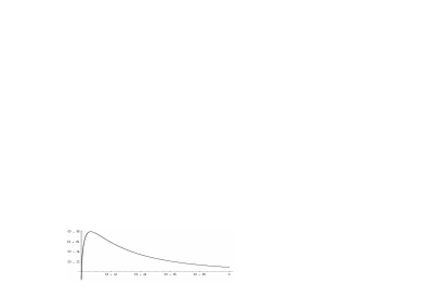
Figure 5: $\epsilon_{0}(r)$ for $r\in[0,1]$ ($r=2\textrm{M}t$),  $\ell=0.71$

Figure 6: $\epsilon_{0}(w)$ with $r=10^{-w}$, $w\in[2,10]$,  $\ell=0.71$

This can be easily understood analyzing the interplay between the two different factors present in the integrand. In fact, $E(\theta)$ oscillates assuming positive and negative values with the same amplitude (Figure 7), while for small values of $r$ the exponential $\exp(-r\cosh\theta)$ is approximately constant on an interval in $\theta$ of order $\ln\frac{1}{r}$, and then falls rapidly to zero. Hence, if we decompose the length of this interval as $\ln\frac{1}{r}=nT+x$, the integration on $nT$ gives roughly zero, while the remaining part corresponds to an integration of $E(\theta)$ on a certain fraction of its period, so that it oscillates depending on the value of $x$.

Figure 7: $E(\theta)$ with $\ell=0.71$

Let us now turn to the reflection amplitude (3.7) with the boundary parameter $h$. In this case the one-point function is given by (3.15) with

$$E(\theta)\;\longrightarrow\;\frac{1-\frac{h^{2}}{2\textrm{M}}-\textrm{sn}\left[\frac{2i\textbf{K}}{\pi}\left(i\frac{\pi}{2}-\theta\right)\right]}{1-\frac{h^{2}}{2\textrm{M}}+\textrm{sn}\left[\frac{2i\textbf{K}}{\pi}\left(i\frac{\pi}{2}-\theta\right)\right]}\,E(\theta)\,.$$ (3.17)

For every $h_{\textrm{min}}\leq h<\infty$, at short distances these correlators do not tend to a given limit, as before. Figure 8 shows the one-point correlator as a function of $r$ for different choices of $h$, in the case $\ell=0.55$. We note that the value $h=h_{\textrm{min}}$ corresponds just to a global change of sign with respect to case of $K_{I}(\theta)$ (equivalent to $h\to\infty$).

Summarizing, the common behaviour shared by all these correlators is not surprising in the light of the previous result about the dependence of the central charge on the scaling variable $\textrm{M}r$, even at short distances. Also in this case, the absence of a proper ultraviolet limit can be related to the fact that the infinite boundary resonance states never decouple from the theory. By using the Form Factors of the magnetic operator computed in [4], it is also easy to see that the same phenomenon occurs for its one–point function of this field.

Figure 8: $\ell=0.55$. One-point function of the energy operator with $(a)$ $h=h_{\textrm{min}}$, $(b)$ $h=1.60\,h_{\textrm{min}}$, $(c)$ $h=1.61\,h_{\textrm{min}}$ and $(d)$ $h=1.73\,h_{\textrm{min}}$.

4 The Sinh-Gordon Model

4.1 The Ordinary Case

The Sinh-Gordon model is defined by the field equation

$$\partial^{2}_{t}\phi-\partial^{2}_{x}\phi+\frac{\sqrt{8}m^{2}}{\beta}\sinh(\sqrt{2}\beta\phi)=0\,\,\,,$$ (4.1)

and has a bulk $S$-matrix of the form ([11])

$$S(\theta)=-\frac{1}{s_{a}(\theta)s_{1-a}(\theta)}\,\,\,,$$ (4.2)

where

$$s_{x}(\theta)=\frac{\sinh\left[\frac{1}{2}(\theta+i\pi x)\right]}{\sinh\left[\frac{1}{2}(\theta-i\pi x)\right]}\,\,\,,$$ (4.3)

and

$$a=\frac{\beta^{2}}{4\pi}\left(\frac{1}{1+\beta^{2}/4\pi}\right)\,\,\,.$$ (4.4)

In the presence of a boundary, this model is integrable if the boundary conditions have the form ([7], [12])

$$\partial_{x}\phi|_{0}=\frac{\sqrt{2}m}{\beta}\left(\varepsilon_{0}e^{-\frac{\beta}{\sqrt{2}}\phi(0,t)}-\varepsilon_{1}e^{\frac{\beta}{\sqrt{2}}\phi(0,t)}\right)\,,$$ (4.5)

where $\varepsilon_{0}$ and $\varepsilon_{1}$ are two boundary parameters, which can be alternatively parameterized by

$$\varepsilon_{i}=\cos\pi a_{i}\qquad\qquad 0\leq a_{1}\leq a_{0}\leq 1\,\,\,.$$ (4.6)

The reflection amplitude can be obtained by analytic continuation from the one of the sine-Gordon breather calculated in [13], and has been analyzed in [14]. It is given by

$$K(\theta)=\frac{s_{\frac{1}{2}}(\theta)s_{\frac{1+a}{2}}(\theta)s_{\frac{2-a}{2}}(\theta)}{s_{\frac{1-E}{2}}(\theta)s_{\frac{1+E}{2}}(\theta)s_{\frac{1-F}{2}}(\theta)s_{\frac{1+F}{2}}(\theta)}\,\,\,,$$ (4.7)

where

$$E=(a_{0}+a_{1})(1-a)\qquad;\qquad F=(a_{0}-a_{1})(1-a)\,\,\,.$$ (4.8)

In the case of Neumann boundary conditions, where $a_{0}=a_{1}=\frac{1}{2}$, eq. (4.7) becomes

$$K(\theta)=\frac{s_{\frac{1+a}{2}}(\theta)}{s_{\frac{1}{2}}(\theta)s_{\frac{a}{2}}(\theta)}\,\,\,.$$ (4.9)

4.2 The Elliptic Case

Let us consider the elliptic $S$-matrix

$$S(\theta,a)=\frac{\textrm{sn}\left[\frac{\textbf{K}}{i\pi}(\theta-i\pi a)\right]}{\textrm{sn}\left[\frac{\textbf{K}}{i\pi}(\theta+i\pi a)\right]}\frac{\textrm{cn}\left[\frac{\textbf{K}}{i\pi}(\theta+i\pi a)\right]}{\textrm{cn}\left[\frac{\textbf{K}}{i\pi}(\theta-i\pi a)\right]}\,\,\,,$$ (4.10)

which has real period $T=2\pi\frac{\textbf{K}^{\prime}}{\textbf{K}}$ and in the ordinary limit ($\ell\to 0$) reduces to the Sinh-Gordon $S$-matrix (4.2).

The analytic structure of $S(\theta,a)$ in shown in Figure 9.

Figure 9: Analytic structure of $S(\theta)$ in the fundamental domain

In [4] it was analyzed the generalization of the roaming limit, which leads to the $S$-matrix of the Ising model $S(\theta)=-1$. In particular, it consists in taking

$$a=m+i(2n+1)\frac{T}{2\pi}+\delta\qquad m\in\mathbb{Z},\,n\in\mathbb{Z}$$ (4.11)

and sending $\delta\rightarrow 0$. The arrows in Figure 9 refer to the case $m=n=0$ and indicate the final positions of poles and zeroes, which cancel each others.

We present now an elliptic reflection amplitude with real period $T^{\prime}=\pi\frac{\textbf{K}^{\prime}}{\textbf{K}}$ and without poles having a real part in the physical strip, which in the ordinary limit tends to the Neumann reflection amplitude of the Sinh-Gordon model (4.9):

$$K(\theta)=K_{I}^{\prime\prime}(\theta)f(\theta)N(\theta)$$ (4.12)

where $K_{I}^{\prime\prime}(\theta)$ is given by (3.9), the factor

$$N(\theta)=\quad\frac{\textrm{sn}\left[\frac{\textbf{K}}{i\pi}\left(\theta-i\frac{\pi}{2}a\right)\right]}{\textrm{sn}\left[\frac{\textbf{K}}{i\pi}\left(\theta+i\frac{\pi}{2}a\right)\right]}\frac{\textrm{sn}\left[\frac{\textbf{K}}{i\pi}\left(\theta+i\frac{\pi}{2}(1+a)\right)\right]}{\textrm{sn}\left[\frac{\textbf{K}}{i\pi}\left(\theta-i\frac{\pi}{2}(1+a)\right)\right]}\,\,\,,$$ (4.13)

is the direct generalization of the ordinary one, and

$$f(\theta)=\left\{\frac{\vartheta_{4}\left[\frac{1}{2i}\left(\theta-i\frac{\pi}{2}a\right)\right]\vartheta_{4}\left[\frac{1}{2i}\left(\theta+i\frac{\pi}{2}(1+a)\right)\right]}{\vartheta_{4}\left[\frac{1}{2i}\left(\theta+i\frac{\pi}{2}a\right)\right]\vartheta_{4}\left[\frac{1}{2i}\left(\theta-i\frac{\pi}{2}(1+a)\right)\right]}\right\}^{2}\,\,\,,$$ (4.14)

is a doubly periodic function necessary to satisfy the crossing equation (2.2), which tends to $1$ as $\ell\rightarrow 0$ (for the properties of Theta functions, see [6]).

The analytic structure of $K(\theta)$ is shown in Figure 10

Figure 10: Analytic structure of $K(\theta)$ in the fundamental domain

It is interesting to note that the initial Ising factor present in (4.12) is the one with period $T^{\prime\prime}=\frac{\pi}{2}\frac{\textbf{K}^{\prime}}{\textbf{K}}$, while (4.12) has altogether period $T^{\prime}=\pi\frac{\textbf{K}^{\prime}}{\textbf{K}}$. This choice, which may not seem very natural, is motivated by the requirement that the roaming limit applied on (4.12) produces the reflection amplitude of the Ising model.

In fact, considering $a=m+i(2n+1)\frac{T}{2\pi}+\delta$, in the limit $\delta\to 0$ poles and zeroes move according to Figure 11, leading to the Ising reflection amplitude (3.8) with period $T^{\prime}$.

Figure 11: Roaming limit $\left(a\to i\frac{T}{2\pi}\right)$

It is now clear the reason why we have to use a reflection amplitude with real period half of the $S$-matrix one. In fact, contrary to the ordinary roaming limit in which $a=1+iC$ and $C\to\infty$, now the imaginary part of $a$ is sent to a finite value $\frac{T}{2\pi}$. Hence, since in the reflection amplitude the parameter $a$ is multiplied by a factor $\frac{1}{2}$ absent in the expression of the $S$-matrix, poles and zeroes are shifted on the real axis by $\frac{T}{4}$ instead of $\frac{T}{2}$, and, in order to reach the same position, at the beginning they have to be located at half the initial distance.

Figure 11 refers to the case $m=n=0$, but the same final situation will take place for any $n\in\mathbb{Z}$ and for $m=0,3\,(\textrm{mod}\,4)$. On the other hand, in the case $m=1,2\,(\textrm{mod}\,4)$ we need to consider an initial $K(\theta)$ with an Ising factor $K_{I}^{\prime}(\theta)$ instead of $K_{I}^{\prime\prime}(\theta)$, recovering at the end $K_{I}^{\prime\prime}(\theta)$.

In principle, it is possible to extend to the elliptic case also the general reflection amplitude (4.7), defining

$$K(\theta)=K_{I}^{\prime\prime}(\theta)f(\theta)G(\theta)\,,$$ (4.15)

where

$$G(\theta) = \frac{\textrm{sn}\left[\frac{\textbf{K}}{i\pi}\left(\theta+i\frac{\pi}{2}(1+a)\right)\right]}{\textrm{sn}\left[\frac{\textbf{K}}{i\pi}\left(\theta-i\frac{\pi}{2}(1+a)\right)\right]}\frac{\textrm{sn}\left[\frac{\textbf{K}}{i\pi}\left(\theta+i\frac{\pi}{2}(2-a)\right)\right]}{\textrm{sn}\left[\frac{\textbf{K}}{i\pi}\left(\theta-i\frac{\pi}{2}(2-a)\right)\right]}$$ (4.16)

$$\times \frac{\textrm{sn}\left[\frac{\textbf{K}}{i\pi}\left(\theta-i\frac{\pi}{2}(1-E)\right)\right]}{\textrm{sn}\left[\frac{\textbf{K}}{i\pi}\left(\theta+i\frac{\pi}{2}(1-E)\right)\right]}\frac{\textrm{sn}\left[\frac{\textbf{K}}{i\pi}\left(\theta-i\frac{\pi}{2}(1+E)\right)\right]}{\textrm{sn}\left[\frac{\textbf{K}}{i\pi}\left(\theta+i\frac{\pi}{2}(1+E)\right)\right]}$$

$$\times \frac{\textrm{sn}\left[\frac{\textbf{K}}{i\pi}\left(\theta-i\frac{\pi}{2}(1-F)\right)\right]}{\textrm{sn}\left[\frac{\textbf{K}}{i\pi}\left(\theta+i\frac{\pi}{2}(1-F)\right)\right]}\frac{\textrm{sn}\left[\frac{\textbf{K}}{i\pi}\left(\theta-i\frac{\pi}{2}(1+F)\right)\right]}{\textrm{sn}\left[\frac{\textbf{K}}{i\pi}\left(\theta+i\frac{\pi}{2}(1+F)\right)\right]}$$

and

$$f(\theta) = \left\{\frac{\vartheta_{4}\left[\frac{1}{2i}\left(\theta+i\frac{\pi}{2}(1+a)\right)\right]}{\vartheta_{4}\left[\frac{1}{2i}\left(\theta-i\frac{\pi}{2}(1+a)\right)\right]}\frac{\vartheta_{4}\left[\frac{1}{2i}\left(\theta+i\frac{\pi}{2}(2-a)\right)\right]}{\vartheta_{4}\left[\frac{1}{2i}\left(\theta-i\frac{\pi}{2}(2-a)\right)\right]}\right\}^{2}$$ (4.17)

$$\times \left\{\frac{\vartheta_{4}\left[\frac{1}{2i}\left(\theta-i\frac{\pi}{2}(1-E)\right)\right]}{\vartheta_{4}\left[\frac{1}{2i}\left(\theta+i\frac{\pi}{2}(1-E)\right)\right]}\frac{\vartheta_{4}\left[\frac{1}{2i}\left(\theta-i\frac{\pi}{2}(1+E)\right)\right]}{\vartheta_{4}\left[\frac{1}{2i}\left(\theta+i\frac{\pi}{2}(1+E)\right)\right]}\right\}^{2}$$

$$\times \left\{\frac{\vartheta_{4}\left[\frac{1}{2i}\left(\theta-i\frac{\pi}{2}(1-F)\right)\right]}{\vartheta_{4}\left[\frac{1}{2i}\left(\theta+i\frac{\pi}{2}(1-F)\right)\right]}\frac{\vartheta_{4}\left[\frac{1}{2i}\left(\theta-i\frac{\pi}{2}(1+F)\right)\right]}{\vartheta_{4}\left[\frac{1}{2i}\left(\theta+i\frac{\pi}{2}(1+F)\right)\right]}\right\}^{2}$$

In order to avoid poles with real part in the physical strip, both the parameters $E$ and $F$ have to lie in the interval $[0,1]$. Furthermore, the roaming limit leads to an Ising reflection factor only for certain specific choices of $E$ and $F$ in terms of $a$.

5 Conclusions

In this paper we have studied the physical effects induced by an infinite number of boundary resonance states in certain integrable quantum field theories. The main result of our analysis regards the ultraviolet regime shown by such kind of theories. We have studied, in particular, in the elliptic generalization of the Ising model, the short–distance behaviour of the effective central charge and of the one–point function of the energy operator, which in the ordinary case scale, respectively, as a constant and as $\frac{1}{r}$. In the elliptic case, instead, both these quantities display oscillations as $r\to 0$, and do not have a definite limit. This leads to the physical interpretation that the infinite resonance states with increasing mass present on the boundary never decouple from the theory, even at very short distances, making meaningless in this case the concept of scaling limit.

The other interesting feature emerged from this work is the crucial role played by the choice of the real periodicity. In fact, various theories with different real periods for the scattering and the reflection amplitudes lead to the same theory in the limit $\ell\to 0$, because the ordinary case corresponds to $T\to\infty$. However, since for $\ell>0$ this period is finite, it is necessary to treat it carefully. Indeed, the roaming limit procedure, which connects the Sinh-Gordon model to the Ising model, can be consistently generalized to the elliptic case only imposing that the reflection amplitude has half real period with respect to the $S$-matrix. This has a physical implication on the nature of the spectra of the theory: once the bulk spectrum of resonance states is given, the boundary one is then automatically fixed.

Acknowledgements

V.R. thanks SISSA for a pre-graduate grant and for hospitality.

References

- [1] Al.B. Zamolodchikov, Resonance Factorized Scattering and Roaming Trajectories, ENS-LPS-335.
- [2] A.B. Zamolodchikov, Symmetric Factorized –Matrix in Two Space–Time Dimensions, Comm. Math. Phys. 69 (1979) 165.
- [3] S. Lukyanov and A.B. Zamolodchikov, Form–Factors of Soliton Creating Operators in the Sine–Gordon Model, hep-th/0102079.
- [4] G. Mussardo and S. Penati, A quantum field theory with infinite resonance states, Nucl. Phys. B 567 (2000) 454.
- [5] O.A. Castro–Alvaredo and A. Fring, Constructing Infinite Particle Spectra, hep-th/0103252.
- [6] I.S. Gradshteyn and I.M. Ryzhik, Table of integrals, series, and products, Academic Press (1992)
- [7] S. Ghoshal and A.B. Zamolodchikov, Boundary -matrix and Boundary State in Two-dimensional Integrable Quantum Field Theory, Int. J. Mod. Phys. A 9 (1994) 3841, Erratum-ibid. A 9 (1994) 4353.
- [8] A. Fring and R. Koberle, Factorized Scattering in the Presence of Reflecting Boundaries, Nucl. Phys. B 421 (1994) 159.
- [9] A. LeClair, G. Mussardo, H. Saleur and S. Skorik, Boundary Energy and Boundary States in Integrable Quantum Field Theories, Nucl. Phys. B 453 (1995) 581.
- [10] R. Konik, A. LeClair and G. Mussardo, On Ising Correlation Functions with Boundary Magnetic Field, Int. J. Mod. Phys. A11 (1996) 2765.
- [11] A.E. Arinshtein, V.A. Fateev and A.B. Zamolodchikov, Quantum S-matrix of the (1+1)-dimensional Todd Chain, Phys. Lett. B 87 (1979) 389.
- [12] A. MacIntyre, Integrable Boundary Conditions for Classical Sine-Gordon Theory, J. Phys. A 28 (1995) 1089.
- [13] S. Ghoshal, Bound State Boundary -matrix of the Sine-Gordon Model, Int. J. Mod. Phys. A 9 (1994) 4801.
- [14] E. Corrigan and A. Taormina, Reflection Factors and a Two Parameter Family of Boundary Bound States in the Sinh-Gordon Model, J. Phys. A 33 (2000) 8739.