SUSX-TH/01-029
hep-th/0106285
Moving Five-Branes in Low-Energy Heterotic M-Theory

We construct cosmological solutions of four-dimensional effective heterotic M-theory with a moving five-brane and evolving dilaton and $T$ modulus. It is shown that the five-brane generates a transition between two asymptotic rolling-radii solutions. Moreover, the five-brane motion always drives the solutions towards strong coupling asymptotically. We present an explicit example of a negative-time branch solution which ends in a brane collision accompanied by a small-instanton transition. The five-dimensional origin of some of our solutions is also discussed.

I Introduction

Brane-world models share a number of characteristic properties which make them a particularly interesting starting point for early universe cosmology. One common feature which has stimulated most of the work on brane-world cosmology [1, 2, 3, 4, 5, 6, 7, 8, 9] to date is the presence of stress energy localised on the brane leading to inhomogeneous additional dimensions. In this paper, we will be concerned with another generic property, namely the possibility that branes move as part of the cosmological evolution. While there have been some early proposals for moving brane cosmological scenarios [10] the problem has only recently received wider attention [11, 12, 13, 14, 15].

Here, we will not be so much concerned with cosmological scenarios but rather with constructing and analysing fundamental cosmological solutions with moving branes in a well-defined M-theory context. More specifically, we will consider heterotic M-theory [16, 17, 18] compactified on a Calabi-Yau three-fold. The resulting five-dimensional theory consists of an $N=1$ bulk supergravity theory on the orbifold $S^{1}/Z_{2}$ coupled to two four-dimensional $N=1$ theories residing on branes which are stuck to the two orbifold planes [19, 20, 21]. In addition, M-theory five-branes can be included in the vacuum of the 11-dimensional theory [16, 22, 23]. These five-branes are transverse to the orbifold direction and wrap complex cycles in the Calabi-Yau three-fold. Therefore, they appear as additional three-branes in the effective $D=5$ theory. Unlike the three-branes on the orbifold fix planes, these additional branes can move in the orbifold direction and it is this new possibility that we wish to analyse in a cosmological context. A five-brane may then collide with one of the boundaries in the course of the cosmological evolution. It is then converted into an instanton located on this boundary through a small-instanton transition [24, 25, 26].

Practically, we will be working in the context of the four-dimensional effective theory, obtained by further reduction on the domain-wall vacuum of the $D=5$ theory [19]. The simplest version of this $D=4$, $N=1$ theory contains three chiral superfields, namely the dilaton $S$, the universal $T$ modulus and the modulus $Z$ which specifies the position of the five-brane in the orbifold direction. This effective action constitutes a generalisation of the standard low-energy action for $E_{8}\times E_{8}$ heterotic string to include the five-bane modulus $Z$. In this paper, we will not explicitly include a non-perturbative superpotential for these moduli but rather focus on the simplest possibility of freely rolling fields.

As we will see, the axions in these superfields can be set to zero consistently. Our problem is then to study the cosmological evolution of the dilaton $\phi$ measuring the Calabi-Yau volume, the real part of the $T$ modulus $\beta$ measuring the orbifold size, the five-brane position $z$ and the scale factor $\alpha$ of the universe. It is immediately clear from the corresponding effective action, that the fields $\phi$ and $\beta$ cannot be set to constants as soon as the five-brane moves. Therefore, the evolution of $z$ cannot be studied in isolation and we must include the standard moduli $\phi$ and $\beta$ in our analysis as well.

Let us briefly summarise our main results. We present a general method of analysing systems with moving branes which is based on a cosmological moduli space Lagrangian [27]. This allows us to find the most general solution for our problem and makes it particularly simple to incorporate a number of generalisations. As usual, the solutions we find each exist for the negative as well as the positive time branch. Asymptotically, at either end of the negative or positive semi-infinite time ranges, our solutions reduce to the standard rolling radii solutions involving $\alpha$, $\beta$ and $\phi$ only. The five-brane is practically at rest in these limits. However, the early and late asymptotic regions correspond to two different rolling radii solutions, in general. The transition between these two solutions is generated by the five-brane which only moves during an intermediate period. Interestingly, not all rolling-radii solutions can be obtained asymptotically but only those which lead to strong coupling. Hence, while there are standard rolling radii solutions which approach weak coupling at one end of the time range, five-brane motion precludes this possibility. Another interesting feature of the solutions is that the five-brane only moves a finite (coordinate) distance. For each solution, one can therefore adjust whether or not the five-brane collides with one of the boundaries. We present an explicit example, where a negative time-branch solution ends with a brane collision accompanied by a small-instanton transition. Our solutions and their generalisations to include the effect of a potential provide a generalised framework for negative time branch cosmologies. As such they form the common ground between the “traditional” dilaton-driven pre-big-bang scenario [28] and the related “ekpyrotic” universe scenario [11] where the dilaton is replaced by the five-brane modulus.

II Four-dimensional effective action

To set the scene, we would first like to present the four-dimensional low-energy effective theory we will be using and explain its relationship to the underlying heterotic M-theory. Of particular importance for the interpretation of our results is the relation to heterotic M-theory in five dimensions, obtained from the 11-dimensional theory by compactification on a Calabi-Yau three-fold. This five-dimensional theory provides an explicit realisation of a brane-world theory.

Our starting point is 11-dimensional Horava-Witten theory [17, 18], that is 11-dimensional supergravity on the orbifold $S^{1}/Z_{2}\times M_{10}$ coupled to two 10-dimensional $E_{8}$ super-Yang-Mills theories each residing on one of the two orbifold fixed planes. Upon compactification of this theory on a Calabi-Yau three-fold to five-dimensions [19, 20] one obtains a five-dimensional $N=1$ gauged supergravity theory on the orbifold $S^{1}/Z_{2}\times M_{4}$. This bulk theory is coupled to two $D=4$, $N=1$ theories which originate from the ten-dimensional $E_{8}$ gauge theories and are localised on three-branes which coincide with the now four-dimensional orbifold fixed planes.

An important fact for the present paper is that in compactifying from 11 to five dimensions, additional five-branes can be included in the vacuum [22, 23]. These five-branes are transverse to the orbifold and wrap (holomorphic) two-cycles within the Calabi-Yau three-fold. Hence, they also appear as three-branes in the five-dimensional effective theory. Unlike the “boundary” three-branes which are stuck to the orbifold fix points, however, these three-branes are free to move in the orbifold direction. Altogether, the five-dimensional theory is then still a gauged $N=1$ supergravity theory on the orbifold $S^{1}/Z_{2}\times M_{4}$. It now couples to the two $N=1$ theories on the boundary three-branes as well as to a series of $N=1$ theories residing on the additional three-branes.

The vacuum of this five-dimensional theory is a non-trivial BPS domain wall solution with an associated effective four-dimensional theory which describes fluctuations around this vacuum state [19]. It is this four-dimensional effective theory, in its most elementary form, which we will use as a starting point for the present paper. First of all, for simplicity, we focus on the case of one additional five- (three)-brane in the bulk. The generalisation of our results to a more complicated configuration is straightforward and will be briefly discussed in the end. For our purpose, we can truncate the four-dimensional theory to three chiral superfields, namely the dilaton $S$, the universal $T$ modulus and the position modulus $Z$ which specifies the position of the additional brane in the orbifold direction. The Kähler potential which governs the dynamics of these fields has been computed in Ref. [23, 29] and is given by

$$K=-\ln\left(S+\bar{S}-q_{5}\frac{(Z+\bar{Z})^{2}}{T+\bar{T}}\right)-3\ln\left(T+\bar{T}\right)\;,$$ (1)

where $q_{5}$ is a constant. Let us briefly explain the meaning of (the bosonic components of) these superfields in terms of the fields in the underlying five-dimensional theory. To do this we introduce the six real fields $(\phi,\sigma)$, $(\beta,\chi)$ and $(z,\zeta)$ through

$$S = e^{\phi}+q_{5}z^{2}e^{\beta}-2i(\sigma-q_{5}z^{2}\chi)$$ (2)

$$T = e^{\beta}+2i\chi$$ (3)

$$Z = e^{\beta}z-2i(\zeta-z\chi)\;.$$ (4)

The field $\phi$ originates from the five-dimensional dilaton which is part of the universal $D=5$ hypermultiplet. It measures the size of internal Calabi-Yau three-fold (averaged over the orbifold) such that the Calabi-Yau volume is given by $ve^{\phi}$ with some fixed reference volume $v$. The corresponding dilatonic axion $\sigma$ is the other zero mode surviving from the universal hypermultiplet. The field $\beta$ is obtained as the zero mode of the $(55)$ component in the $D=5$ metric and as such measures the size of the orbifold. More precisely, this size is given by $\pi\rho e^{\beta}$ with a fixed reference size $\pi\rho$. The associated axion $\chi$ is related to the vector field in the five-dimensional gravity multiplet. Finally, the field $z$ originates from the world-volume of the additional three-brane and specifies the position of this brane in the orbifold direction. We have normalised this field to the interval

$$z\in[0,1]$$ (5)

where the two endpoints $z=0$ and $z=1$ correspond to the locations of the boundary branes. The associated axion $\zeta$ also originates from the additional three-brane and it is related to the self-dual two-form of the underlying five-brane. The constant $q_{5}$ in the above Kähler potential can be written as

$$q_{5}=\pi\epsilon_{0}\beta_{5}$$ (6)

where $\beta_{5}$ is the five-brane charge and $\epsilon_{0}$ is defined by

$$\epsilon_{0}=\left(\frac{\kappa}{4\pi}\right)^{2/3}\frac{2\pi\rho}{v^{2/3}}\;.$$ (7)

Here, $\kappa$ is the 11-dimensional Newton constant while $v$ and $\pi\rho$ have been introduced above. We note that the five-brane charge and, hence, the constant $q_{5}$ needs to be positive if the compactification is to preserve four-dimensional supersymmetry, as we have assumed.

The above Kähler potential is a lowest order expression in the strong-coupling expansion parameter $\epsilon$ defined by

$$\epsilon=\epsilon_{0}e^{\beta-\phi}\;.$$ (8)

This quantity measures the size of the loop corrections to the four-dimensional effective action, or, from a five-dimensional viewpoint, the warping of the domain wall vacuum solution. While the $S$, $T$ part of the Kähler potential does not receive any corrections at first order [30] in $\epsilon$, such corrections are expected for the $Z$-dependent part. To date, these corrections have not been computed and we will work with the lowest order expression which is valid as long as $\epsilon$ is sufficiently small.

When the five-brane collides with one of the boundaries, that is, if $z\rightarrow 0$ or $z\rightarrow 1$, one expects the appearance of new massless states which originate from membranes stretched between the five-brane and its $Z_{2}$ mirror and the five-brane and the boundary. The theory then undergoes a small-instanton transition [24, 25, 26], where the bulk five-brane is converted into an instanton (or a gauge five-brane) on the boundary. The particle content and other properties of the $N=1$ theory on the relevant boundary can change dramatically under this transition. At present, the dynamics are not well enough understood to be able to follow the cosmological evolution through this transition without additional ad-hoc assumptions. Here, we will not attempt to improve on this but we will merely analyse the conditions under which a brane-collision occurs.

Perturbatively, the superpotential for the moduli fields $S$, $T$ and $Z$ vanishes but non-trivial contributions are, of course, expected at the non-perturbative level [31, 32, 33, 34]. While there is a long history of analysing the phenomenology of non-perturbative superpotentials for $S$ and $T$, particularly those induced by gaugino condensation, only recently first efforts have been made to include the modulus $Z$ [11, 14, 15]. While this is an interesting direction for future research, here we focus on the simplest case of a vanishing superpotential. In our cosmological context, this amounts to finding generalisations of rolling-radii solutions to include the position modulus $Z$. In general, rolling-radii solutions constitute a basic and important class of string cosmological solutions and appear to be the natural starting point for a study of moving-brane cosmologies.

The component action of our model can be straightforwardly computed from the Kähler potential (1) together with the reparametrisation (3). To fix our conventions, we provide the relevant terms in the supergravity action which are given by

$$S=\frac{1}{2\kappa_{P}^{2}}\int\sqrt{-g}\left[\frac{1}{2}R+K_{\imath{\bar{\jmath}}}\partial_{\mu}\Phi^{\imath}\partial^{\mu}\bar{\Phi}^{\bar{\jmath}}\right]\;.$$ (9)

Here $K_{\imath\bar{\jmath}}=\partial^{2}K/\partial\Phi^{\imath}\partial\bar{\Phi}^{\bar{\jmath}}$ is the Kähler metric and $(\Phi^{\imath})=(S,T,Z)$. In terms of higher-dimensional quantities, the four-dimensional Newton constant $\kappa_{P}$ can be expressed as

$$\kappa_{P}^{2}=\frac{\kappa^{2}}{2\pi\rho v}\;.$$ (10)

It can be seen that all terms in the resulting component action are at least bilinear in the axion fields $\sigma$, $\chi$ and $\zeta$. Therefore, these fields can be consistently set to zero and we can work with an action that is further truncated to the fields $\phi$, $\beta$ and $z$. The component action then reads

$$S=-\frac{1}{2\kappa_{P}^{2}}\int\sqrt{-g}\left[\frac{1}{2}R+\frac{1}{4}\partial_{\mu}\phi\partial^{\mu}\phi+\frac{3}{4}\partial_{\mu}\beta\partial^{\mu}\beta+\frac{q_{5}}{2}e^{\beta-\phi}\partial_{\mu}z\partial^{\mu}z\right]\;.$$ (11)

It is for this simple action that we wish to study cosmological solutions in the following sections. Due to the non-trivial kinetic term for $z$, solutions with exactly constant $\phi$ or $\beta$ do not exist as soon as the five-brane moves. Therefore, the evolution of all three fields is linked and (except for setting $z=$ const) cannot be truncated consistently any further. Recently, this has also been pointed out in Ref. [15]. We remark that this statement remains true in the presence of a non-perturbative superpotential.

III Cosmological solutions with a moving five-brane

Let us now look for cosmological solutions to the field equations derived from the action (11). For simplicity, we assume the three-dimensional spatial space to be flat. Our Ansatz then reads

$$ds^{2} = -e^{2\nu}d\tau^{2}+e^{2\alpha}d{\bf x}^{2}$$ (12)

$$\phi = \phi(\tau)$$ (13)

$$\alpha = \alpha(\tau)$$ (14)

$$\beta = \beta(\tau)$$ (15)

$$z = z(\tau)$$ (16)

Later on, we will indicate how to include three-dimensional spatial curvature. The equation of motion for $z$ can be immediately integrated once, leading to

$$\dot{z}=ve^{-3\alpha+\nu-\beta+\phi}\;,$$ (17)

where the dot denoted the derivative with respect to $\tau$. This result may be substituted back into the rest of the system to obtain a closed set of equations for $\alpha$, $\beta$ and $\phi$. These equations can then be integrated in a manner closely analogous to the formalism for anti-symmetric tensor fields in cosmology developed in Ref. [27]. We will subsequently use this formalism which makes the general structure of the equations and their solutions particularly transparent. Also, several generalisations to be discussed later are most easily incorporated in this language.

A Equations of motion and their solutions

It turns out that the remaining equations of motion for our system can written in the elegant form

$$\frac{d}{d\tau}\left(EG{\mbox{\boldmath$\alpha$}}^{\prime}\right)+E^{-1}\frac{\partial U}{\partial{\mbox{\boldmath$\alpha$}}} = 0$$ (18)

$$\frac{1}{2}E{{\mbox{\boldmath$\alpha$}}^{\prime}}^{T}G{\mbox{\boldmath$\alpha$}}^{\prime}+E^{-1}U = 0\;.$$ (19)

Here, the scale factors have been arranged in a vector ${\mbox{\boldmath$\alpha$}}=\left(\alpha,\beta,\phi\right)$ which spans the moduli space of our cosmological model. The potential $U$ on this moduli space is given by

$$U=\frac{1}{2}u^{2}e^{{\bf q}.{\mbox{\boldmath$\alpha$}}}\;,\qquad u^{2}=\frac{q_{5}v^{2}}{2}\;$$ (20)

where the vector ${\bf q}$ is given by ${\bf q}=(0,-1,1)$. Further, the “Einbein” $E$ is defined by $E=e^{-\nu+{\bf d}\cdot{\mbox{\boldmath$\alpha$}}}$ with the dimension vector ${\bf d}=(3,0,0)$ and we have introduced a metric $G={\rm diag}\left(-3,\frac{3}{4},\frac{1}{4}\right)$. Clearly, these field equations can be obtained from the Lagrangian

$${\cal L}=\frac{1}{2}E{{\mbox{\boldmath$\alpha$}}^{\prime}}^{T}G{\mbox{\boldmath$\alpha$}}^{\prime}-E^{-1}U$$ (21)

which encodes the dynamics on our moduli space in a compact form. The presence of the potential $U$ is a direct consequence of the five-brane motion and its five-brane origin is encoded in the characteristic vector ${\bf q}$. In more complicated situations, for example when spatial curvature is included, the potential $U$ consists of more than one exponential. Even then, the Lagrangian (21) can sometimes be solved by employing Toda theory. We will return to such generalisations later on.

However, for now, we are dealing with the simple potential (20) containing one exponential due to the moving five-brane only. This system can always be integrated [27] and the general solution in the comoving gauge, $\nu=0$, written in vector notation, is given by

$${\mbox{\boldmath$\alpha$}}={\bf p}_{i}\ln\left|\frac{t-t_{0}}{T}\right|+\left({\bf p}_{f}-{\bf p}_{i}\right)\ln\left(\left|\frac{t-t_{0}}{T}\right|^{-\delta}+1\right)^{-\frac{1}{\delta}}+{\mbox{\boldmath$\alpha$}}_{0}$$ (22)

$$z=d\left(1+\left|\frac{T}{t-t_{0}}\right|^{-\delta}\right)^{-1}+z_{0}\;,$$ (23)

where $t$ is the proper time. Let us discuss the various integration constants in this solution. The time-scales $t_{0}$ and $T$ are clearly arbitrary as are the constants $d$ and $z_{0}$ which parameterise the motion of the five-brane. In contrast, the initial and final “expansion powers” ${\bf p}_{i}$ and ${\bf p}_{f}$ each satisfy the two constraints

$${\bf p}_{n}G{\bf p}_{n}=0\;,\qquad{\bf p}_{n}\cdot{\bf d}=1\;,$$ (24)

where $n=i,f$, and, moreover, they are mapped into one another by

$${\bf p}_{f}={\bf p}_{i}+\delta\frac{2G^{-1}{\bf q}}{<{\bf q},{\bf q}>}\;.$$ (25)

Here, the scalar product $<\cdot,\cdot>$ is defined by $<a,b>={\bf a}^{T}G^{-1}{\bf b}$. The power $\delta$ is defined by

$$\delta=-{\bf q}\cdot{\bf p}_{i}\;.$$ (26)

We note that the map (25) and the conditions (24) are consistent with one another in the sense that ${\bf p}_{f}$ as given by Eq. (25) will always satisfy the constraints (24) as long as the vector ${\bf p}_{i}$ does. As a consequence, the six expansion powers contained in ${\bf p}_{i}$ and ${\bf p}_{f}$ depend on one independent degree of freedom. Finally, the additive constants ${\mbox{\boldmath$\alpha$}}_{0}$ are subject to one further condition

$${\bf q}\cdot{\mbox{\boldmath$\alpha$}}_{0}=\ln\left(\frac{d^{2}q_{5}<{\bf q},{\bf q}>}{8}\right)\;.$$ (27)

Altogether, we have seven independent integration constants as expected on general grounds.

In order for the logarithms in Eq. (22) to be well defined the range of $t$ should be restricted to

$$t\in\left\{\begin{array}[]{clll}\left[-\infty,t_{0}\right]\;,&(-)\;{\rm branch}\\ \left[t_{0},+\infty\right]\;,&(+)\;{\rm branch}\end{array}\right.\;.$$ (28)

As usual, we, therefore, find a positive and a negative time branch for each solution. One can easily verify that the former always starts out in a past curvature singularity while the latter ends in a future curvature singularity.

A useful observation is that each of the above solutions is invariant under the mapping

$${\bf p}_{i}\rightarrow{\bf p}_{f}\;,\quad{\bf p}_{f}\rightarrow{\bf p}_{i}\;,\quad d\rightarrow-d\;,\quad z_{0}\rightarrow z_{0}+d\;.$$ (29)

At the same time, this map implies a sign change $\delta\rightarrow-\delta$ as can be seen from Eq. (25) and (26). In order to avoid having two different sets of integration constants associated to each solution we can, therefore, fix the sign of the parameter $\delta$. It proves convenient to adopt the convention

$$\begin{array}[]{cc}\delta>0\qquad(-)\;{\rm branch}\\ \delta<0\qquad(+)\;{\rm branch}\end{array}$$ (30)

Finally, for the sake of concreteness, let us present the explicit form of our solutions by inserting the particular values for the various general quantities which we have defined. From Eq. (22) the scale factors can be written in component form as

$$\alpha = \frac{1}{3}\ln\left|\frac{t-t_{0}}{T}\right|+\alpha_{0}$$ (31)

$$\beta = p_{\beta,i}\ln\left|\frac{t-t_{0}}{T}\right|+(p_{\beta,f}-p_{\beta,i})\ln\left(\left|\frac{t-t_{0}}{T}\right|^{-\delta}+1\right)^{-\frac{1}{\delta}}+\beta_{0}$$ (32)

$$\phi = p_{\phi,i}\ln\left|\frac{t-t_{0}}{T}\right|+(p_{\phi,f}-p_{\phi,i})\ln\left(\left|\frac{t-t_{0}}{T}\right|^{-\delta}+1\right)^{-\frac{1}{\delta}}+\phi_{0}$$ (33)

while the expression (23) for the five-brane modulus remains unchanged. We see that both expansion powers for the scale factor $\alpha$ are given by $1/3$, a fact which is expected in the Einstein frame and can easily be deduced from the second equation (24). The initial and final expansion powers for $\beta$ and $\phi$ are less trivial and are subject to the first constraint (24) which explicitly reads

$$3p_{\beta,n}^{2}+p_{\phi,n}^{2}=\frac{4}{3}$$ (34)

for $n=i,f$. From Eq. (25) it follows that they are mapped into one another by

$$\left(\begin{array}[]{c}p_{\beta,f}\\ p_{\phi,f}\end{array}\right)=P\left(\begin{array}[]{c}p_{\beta,i}\\ p_{\phi,i}\end{array}\right)\;,\qquad P=\frac{1}{2}\left(\begin{array}[]{rr}1&1\\ 3&-1\end{array}\right)\;.$$ (35)

We note that this map is its own inverse, that is $P^{2}=1$, which is a simple consequence of time reversal symmetry. The power $\delta$ is explicitly given by

$$\delta=p_{\beta,i}-p_{\phi,i}\;.$$ (36)

Finally, the condition (27) takes the explicit form

$$\phi_{0}-\beta_{0}=\ln\left(\frac{2q_{5}d^{2}}{3}\right)\;.$$ (37)

B Properties and asymptotic behaviour of the solutions

Let us now discuss the physical properties of our solutions in some detail. For both branches, the system behaves in a particularly simple manner at either end of the allowed t ranges. In these limits it is easy to see from our solution as presented in equation (22) that the ’Hubble parameters’ can be written as,

$${\bf H}\equiv\dot{{\mbox{\boldmath$\alpha$}}}\simeq\frac{{\bf p}}{t-t_{0}}$$ (38)

with constant expansion coefficients ${\bf p}$ satisfying,

$${\bf p}G{\bf p}=0\;,\quad{\bf d}\cdot{\bf p}=1\;.$$ (39)

In view of our convention (30), the expansion power ${\bf p}$ in these relations is given by ${\bf p}={\bf p}_{i}$ at early times (that is, at $t\rightarrow-\infty$ in the $(-)$ branch and $t\rightarrow t_{0}$ in the $(+)$ branch) and by ${\bf p}={\bf p}_{f}$ at late time (that is, at $t\rightarrow t_{0}$ in the $(-)$ branch and $t\rightarrow\infty$ in the $(+)$ branch). The above relations characterise the standard rolling radii solutions for $\alpha$, $\beta$ and $\phi$ which have been used as a basis for pre-big-bang cosmology [36]. They can be obtained as exact solutions of the action (11) when the five-brane is taken to be static. Their appearance as asymptotic limits of our full solutions can be understood from the five-brane evolution (23). This equation shows that, asymptotically, the five-brane does not move and effectively drops out of the dynamics thereby leaving us with freely rolling radii in these limits. This demonstrates that our solutions show inflationary behaviour at least in some region of the negative time branch.

Thus, we arrive at the following interpretation for our solutions. At early time, the system starts in the rolling radii solution characterised by the initial expansion powers ${\bf p}_{i}$ while the five-brane is practically at rest. When time approaches $|t-t_{0}|\sim|T|$ the five-brane starts to move significantly which leads to an intermediate period with a more complicated evolution of the system. Then, after a finite comoving time, in the late asymptotic region, the five-brane comes to a rest and the scale factors evolve according to another rolling radii solution with final expansion powers ${\bf p}_{f}$. Hence the five-brane generates a transition from one rolling radii solution into another one, a process which is formally described by the map (35). To illustrate the situation, in Fig. 1, we have plotted the allowed expansion powers for rolling radii solutions in the $p_{\beta}$–$p_{\phi}$ plane. The arrows indicate the map between early and late expansion powers generated by the five-brane.

FIG. 1.: It is shown how the ellipse of possible expansion powers $(p_{\beta},p_{\phi})$ is mapped into itself under the influence of the moving five-brane. Points related by the map may be joined with a straight line of slope $-3$ as indicated by the arrows. There are two fixed points under this map on the ellipse given by $\delta=p_{\beta}-p_{\alpha}=0$. These points correspond to solutions which are related to separating solutions in five dimensions. In these special cases the five-brane modulus $z$ is constant.

An obvious question to ask is whether all of the rolling radii solutions represented by the ellipse in Fig. 1 are available as asymptotic limits at, say, early time. Perhaps surprisingly, the answer is no. As can be seen from Eq. (30), the expansion powers at early time are subject to the constraint

$$p_{\beta,i}-p_{\phi,i}=\delta\;\left\{\begin{array}[]{lll}>0&&(-)\;{\rm branch}\\ <0&&(+)\;{\rm branch}\end{array}\right.$$ (40)

Therefore only the solid (dashed) half of the ellipse is available as the early time limit in the negative (positive) time branch. This can also be understood from the consistency requirement that the kinetic energy of $\beta$ and $\phi$ be much larger than the kinetic energy of the five-brane modulus asymptotically if the system is to approach a rolling radii solution. In fact, it can be easily seen that the ratio of these kinetic energies is proportional to the strong coupling expansion parameter $\epsilon$ defined in Eq. (8). For our set of solutions, the asymptotic time evolution of this parameter is specified by

$$\epsilon\sim\left\{\begin{array}[]{lll }|t-t_{0}|^{\delta_{i}}&&{\rm early}\\ |t-t_{0}|^{\delta_{f}}&&{\rm late}\end{array}\right.$$ (41)

where we have defined

$$\delta_{i}=\delta=-{\bf q}\cdot{\bf p}_{i}\;,\qquad\delta_{f}=-\delta_{i}=-{\bf q}\cdot{\bf p}_{f}\;.$$ (42)

We see that, the sign of the $\epsilon$ expansion power is inverted as we go from the early to the late asymptotic region. If we pick a solution with the “wrong” sign, for example a $\delta_{i}<0$ solution at early times in the minus branch, the share of the five-brane kinetic energy increases as $t-t_{0}\rightarrow-\infty$ which is inconsistent with the rolling radii nature of the solutions in this limit. Hence such solutions do not exist and we are restricted to the cases which respect (40). As a consequence, $\epsilon$ always grows asymptotically. This implies growing loop corrections asymptotically or, equivalently, an increasing warping in the orbifold direction. Hence, while there are perfectly viable rolling radii solutions which become weakly coupled in at least one of the asymptotic regions, the presence of a moving five-brane always leads to strong coupling asymptotically. A similar phenomenon has been observed when axion dynamics is added to the simple rolling radii set-up [36, 37].

We note that there two exceptional solutions, indicated by the solid dots in Fig. 1, which are the fix points under the map (35). In other words, for those solutions the early and late expansion powers are identical. It is clear from Eq. (25) that those solutions are characterised by $\delta=0$ or, equivalently, by $p_{\beta}=p_{\phi}=\pm\frac{1}{\sqrt{3}}$. Hence, for those solutions the orbifold and the Calabi-Yau space always evolve at the same rate and the size of the loop corrections is time-independent. However, it follows from Eq. (23) that also the five-brane is static in this case, so that these are really ordinary rolling radii solutions. They correspond to the two separating cosmological solutions of five-dimensional heterotic M-theory found in Ref. [1]. In conclusion, despite these exceptional cases, it remains true that the solutions are always driven to strong coupling asymptotically as soon as the five-brane moves.

Our simple effective action (11) remains valid only as long as loop and higher derivative corrections are sufficiently small and this limits the validity of our solutions in the usual way. Another, perhaps more interesting event leading to a break-down of the effective action is the collision of the five-brane with one of the boundaries, that is $z\rightarrow 0,1$. In this context, an important observation from Eq. (23) is, that the five-brane moves a finite coordinate distance given by $|d|$, only. Consequently, whether or not a brane collision takes place, depends on the choices for the arbitrary integration constants $d$ and $z_{0}$. This may be surprising, perhaps, as one could have expected that a collision is unavoidable in a cosmological setting and in the absence of any stabilising potentials. Of course, this is related to the system always becoming strong-coupling asymptotically which implies that the non-trivial kinetic term for five-brane modulus leads to damping terms in the $z$ equation of motion. We also remark that, for each solution, the five-brane can move in either direction, as specified by the sign of $d$. It can, therefore, collide with either one of the boundaries. This is, of course, a direct consequence of our simple effective action (11) which is invariant under $z\rightarrow-z$ and does not single out a particular direction.

IV An explicit example

We would now like to illustrate our general results by an explicit example. For concreteness, we focus on the negative-time branch and consider the solutions with an approximately static orbifold at early time. In the context of our formalism, these solutions can be singled out by setting the initial expansion power of the orbifold to zero, that is $p_{i,\beta}=0$. From Eq. (34) this implies two possibilities for the initial expansion power of the dilaton, namely $p_{i,\phi}=\pm\frac{2}{\sqrt{3}}$. Only one of these two expansion powers, $p_{i,\phi}=-\frac{2}{\sqrt{3}}$, leads to a positive value for $\delta=p_{i,\beta}-p_{i,\phi}=\frac{2}{\sqrt{3}}$ and can, therefore, be realised as the early time limit of one of our solutions in the negative time branch. Using the map (25), the complete set of initial and final expansion powers for our example is then given by

$${\bf p}_{i}=\left(\begin{array}[]{c}\frac{1}{3}\\ 0\\ -\frac{2}{\sqrt{3}}\end{array}\right)\quad\longrightarrow\quad{\bf p}_{f}=\left(\begin{array}[]{c}\frac{1}{3}\\ -\frac{1}{\sqrt{3}}\\ \frac{1}{\sqrt{3}}\end{array}\right)\;.$$ (43)

Recall here that the first entry in those vectors specifies the expansion power of the scale factor $\alpha$ (which always equals $\frac{1}{3}$) while the second and third entry refer to $\beta$ and $\phi$, respectively.

FIG. 2.: Time-behaviour of $\beta$ (upper curve) and $\phi$ (lower curve) for the example specified in the text.

At early times, $|t-t_{0}|\gg|T|$, the evolution is basically of power-law type with powers ${\bf p}_{i}$. As discussed, this happens because at early time the five-brane is effectively frozen at $z\simeq d+z_{0}$ and does not contribute a substantial amount of kinetic energy. This changes dramatically once we approach the time $|t-t_{0}|\sim|T|$. In a transition period around this time, the brane moves from its original position by a total distance $d$ and ends up at $z\simeq z_{0}$. At the same time, this changes the behaviour of the moduli $\beta$ and $\phi$ until, at late time $|t|\ll|T|$, they correspond to another rolling radii solution with powers controlled by ${\bf p}_{f}$. Concretely, the orbifold size described by $\beta$ turns from being approximately constant at early time to expanding at late time, while the Calabi-Yau size controlled by $\phi$ undergoes a transition from expansion to contraction. This behaviour has been illustrated in Fig. 2.

Recall from Eq. (41) that the expansion powers of the strong coupling expansion parameter $\epsilon$ in the initial and final asymptotic regions are given by $\delta_{n}=p_{\beta,n}-p_{\phi,n}$, where $n=i,f$. We have also seen in general that the transition induced by the brane is simply inverts the sign of this expansion power, so that $\delta_{f}=-\delta_{i}$. For our example, we find

$$\delta_{i}=2/\sqrt{3}\rightarrow\delta_{f}=-2/\sqrt{3}$$ (44)

so that $\epsilon$ decreases initially and increases after the transition. Consequently, the solution runs into strong coupling in both asymptotic regions $t-t_{0}\rightarrow-\infty$ and $t-t_{0}\rightarrow 0$ which illustrates our general result.

Of course, the range of validity of our solution is constrained by loop corrections, as well as higher curvature corrections, in a way that depends on the various integration constants involved. If the constants $d$ and $z_{0}$, characterising the five-brane motion, are chosen such that the five-brane does not collide with the boundary there is no further constraint. As discussed, this can always be arranged. However, we may also choose $d$ sufficiently large so that the five-brane does collides with one of the boundaries. Then the system undergoes a small-instanton transition and our classical solution is invalidated. This typically happens at the time $|t-t_{0}|\simeq|T|$ when the five-brane moves significantly. Depending on integration constants this may happen well before loop and higher-derivative corrections become relevant. In Fig. 3 we have shown a particular case for our example which leads to brane collision. The five-brane is initially located at $d+z_{0}\simeq 0.9$ and moves a total distance of $d=1.5$ colliding with the boundary at $z=0$ at the time $|t-t_{0}|/|T|\simeq 1$.

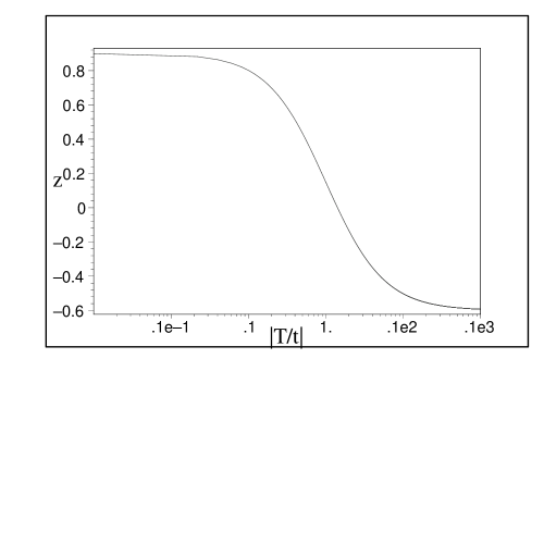
FIG. 3.: Time-behaviour of the five-brane position modulus $z$ for the example specified in the text. The boundaries are located at $z=0,1$ and the five-brane collides with the $z=0$ boundary at $|t/T|\simeq 1$.

This represents an explicit example of a negative-time branch solution which ends in a small-instanton brane-collision.

V Generalisations and Outlook

In this paper, we have presented and analysed the simplest class of cosmological solutions with moving five-branes in the context of four-dimensional effective heterotic M-theory. Clearly, there are a number of interesting generalisations and refinements some of which we would briefly like to discuss below.

• Including spatial curvature : Consider the case where, in addition to the elements included in the above discussion, we wish to include three-dimensional spatial curvature. One of the benefits of our general formalism is that this can be easily incorporated. One can simply continue to work with a moduli space Lagrangian of the form (21). The only change is that another exponential term proportional to $\exp({\bf q}_{c}\cdot{\mbox{\boldmath$\alpha$}})$ which accounts for the spatial curvature has to be added to the potential $U$. The characteristic vector ${\bf q}_{c}$ of this curvature term is different from the corresponding five-brane vector and is explicitly given by ${\bf q}_{c}=(4,0,0)$. Hence, the five-brane and curvature characteristic vectors are orthogonal with respect to our scalar product, that is, $<{\bf q},{\bf q}_{c}>=0$. Therefore, the system can be identified as an $SU(2)^{2}$ Toda model which can be integrated. In a different, but formally similar context, this has been explicitly carried out in Ref. [27].

• Add a perfect fluid : One may want to consider the cosmology of our simple model in the additional presence of a perfect fluid. As before, this can be done by simply adding an exponential term to the potential $U$. The characteristic vector for a perfect fluid with equation of state $p=w\rho$, where $w$ is a constant, is given by ${\bf q}_{\rm fluid}=(3(1-w),0,0)$ which is again orthogonal to the five-brane vector. Hence this situation is again described by an $SU(2)^{2}$ Toda model.

• More than one five-brane : We may also easily generalise our results to include more than one five brane. This simply involves including more potential terms with ${\bf q}=(0,-1,1)$. This, of course, simply amounts to replacing the expression for the normalisation $u^{2}$ of the potential $U$ in Eq. (20) by a generalisation which involves summing over all five-branes. Most of the qualitative features of our solutions will then be unchanged. In particular, all five-branes ’move at the same time’ collectively generating the transition between the two asymptotic regions. However, the initial position and the total distance of the motion can be different for the various five-branes. For example, some of the five-branes may collide with a boundary while the others do not. Of course the five-branes may also collide with one another.

• Include axions : Another obvious generalisation to attempt would be to try and include non-trivial axion dynamics in our solutions. In more simple string cosmology settings without five-branes this has been possible due to an $SL(2)$ symmetry of the string effective action [36, 37]. This symmetry allowed solutions with non-trivial axion dynamics to be generated from systems where the axion fields had been set to zero. However, the presence of the five-brane modulus $Z$ complicates the situation significantly. The only parts of $SL(2)$ which are obviously respected by the Kähler potential (1) are the axionic shift symmetries which do not lead new solutions. It is not clear, at present, whether the Kähler potential (1) has any further symmetries which could be used to generate new cosmological solutions from the ones obtained in this paper.

• Small instanton transition : Finally, an understanding of the dynamics of the small instanton transition whereby a five brane is emitted from or absorbed onto one of the fix point branes would be extremely useful. It would allow us to describe the system as it evolves through the transition which is vital in order to construct “complete” cosmological models.

• Fluctuations : It is known [35, 36] that there exist special rolling radii solutions which, in the context of pre-big-bang inflation, lead to perturbations consistent with a Harrison-Zeldovich spectrum. It is, therefore, expected that such cases with an acceptable fluctuation spectrum also exist in our generalised framework with moving five-branes. We will be analysing this in more detail.

Another possible direction for future work would be a search for five dimensional moving brane solutions of various kinds, including those that correspond to the four dimensional ones found here. It is, of course, straightforward to “oxidise” all our four-dimensional solutions to approximate solutions of five-dimensional heterotic M-theory following the procedure described in Ref. [3]. However, finding the exact solutions in five dimensions in the presence of additional five-branes is a much more difficult task. We have seen that the five-brane is static for the two exceptional solutions with $\delta=0$. In this sense, they are trivial extensions of $D=4$ rolling radii solutions. Finding their $D=5$ counterpart, however, is less trivial, since the presence of the additional five-brane changes the warping of the $D=5$ domain wall, an effect which is not directly visible in $D=4$. However, one can verify that the two separating $D=5$ cosmological solutions found in Ref. [1] can indeed be generalised to include five-branes. Hence, the $D=5$ counterparts of our two exceptional solutions can be obtained as exact solutions. More generally, we have shown that there exist only three $D=5$ solutions, based on the bulk BPS domain wall solution of Ref. [19], which include a single five-brane. These are the BPS domain wall solution with a single five-brane itself and the two aforementioned cosmological solutions. Hence, lifting the other solutions we have presented to exact $D=5$ solutions is not straightforward and requires the study of more complicated metrics in the bulk such as those found in Ref’s [38, 39].

Acknowledgements
A. L. is supported by a PPARC Advanced Fellowship. J. G.  is supported by PPARC.

REFERENCES

- [1] A. Lukas, B. A. Ovrut and D. Waldram, “Cosmological solutions of Horava-Witten theory,” Phys. Rev. D 60 (1999) 086001 [hep-th/9806022].
- [2] L. Randall and R. Sundrum, “An alternative to compactification,” Phys. Rev. Lett. 83 (1999) 4690 [hep-th/9906064].
- [3] A. Lukas, B. A. Ovrut and D. Waldram, “Boundary inflation,” Phys. Rev. D 61 (2000) 023506 [hep-th/9902071].
- [4] P. Binetruy, C. Deffayet, U. Ellwanger and D. Langlois, “Brane cosmological evolution in a bulk with cosmological constant,” Phys. Lett. B 477 (2000) 285 [hep-th/9910219].
- [5] C. Csaki, M. Graesser, L. Randall and J. Terning, “Cosmology of brane models with radion stabilization,” Phys. Rev. D 62 (2000) 045015 [hep-ph/9911406].
- [6] D. Ida, “Brane-world cosmology,” JHEP 0009 (2000) 014 [gr-qc/9912002].
- [7] S. W. Hawking, T. Hertog and H. S. Reall, “Brane new world,” Phys. Rev. D 62 (2000) 043501 [hep-th/0003052].
- [8] B. Carter and J. Uzan, “Reflection symmetry breaking scenarios with minimal gauge form coupling in brane world cosmology,” [gr-qc/0101010].
- [9] C. Deffayet, “Cosmology on a brane in Minkowski bulk,” Phys. Lett. B 502 (2001) 199 [hep-th/0010186].
- [10] G. Dvali and S. H. Tye, “Brane inflation,” Phys. Lett. B 450 (1999) 72 [hep-ph/9812483].
- [11] J. Khoury, B. A. Ovrut, P. J. Steinhardt and N. Turok, “The ekpyrotic universe: Colliding branes and the origin of the hot big bang,” [hep-th/0103239].
- [12] R. Kallosh, L. Kofman and A. Linde, “Pyrotechnic universe,” [hep-th/0104073].
- [13] C. P. Burgess, M. Majumdar, D. Nolte, F. Quevedo, G. Rajesh and R. J. Zhang, “The inflationary brane-antibrane universe,” [hep-th/0105204].
- [14] J. Khoury, B. A. Ovrut, P. J. Steinhardt and N. Turok, “A brief comment on ’The pyrotechnic universe’,” [hep-th/0105212].
- [15] R. Kallosh, L. Kofman, A. Linde and A. Tseytlin, “BPS Branes in Cosmology,” [hep-th/0106241].
- [16] E. Witten, “Strong Coupling Expansion Of Calabi-Yau Compactification,” Nucl. Phys. B 471 (1996) 135 [hep-th/9602070].
- [17] P. Horava and E. Witten, “Heterotic and type I string dynamics from eleven dimensions,” Nucl. Phys. B 460 (1996) 506 [hep-th/9510209].
- [18] P. Horava and E. Witten, “Eleven-Dimensional Supergravity on a Manifold with Boundary,” Nucl. Phys. B 475 (1996) 94 [hep-th/9603142].
- [19] A. Lukas, B. A. Ovrut, K. S. Stelle and D. Waldram, “The universe as a domain wall,” Phys. Rev. D 59 (1999) 086001 [hep-th/9803235].
- [20] A. Lukas, B. A. Ovrut, K. S. Stelle and D. Waldram, “Heterotic M-theory in five dimensions,” Nucl. Phys. B 552 (1999) 246 [hep-th/9806051].
- [21] A. Lukas and K. S. Stelle, “Heterotic anomaly cancellation in five dimensions,” JHEP 0001 (2000) 010 [hep-th/9911156].
- [22] A. Lukas, B. A. Ovrut and D. Waldram, “Non-standard embedding and five-branes in heterotic M-theory,” Phys. Rev. D 59 (1999) 106005 [hep-th/9808101].
- [23] J. Derendinger and R. Sauser, “A five-brane modulus in the effective N = 1 supergravity of M-theory,” Nucl. Phys. B 598 (2001) 87 [hep-th/0009054].
- [24] E. Witten, “Small Instantons in String Theory,” Nucl. Phys. B 460 (1996) 541 [hep-th/9511030].
- [25] O. J. Ganor and A. Hanany, “Small Instantons and Tensionless Non-critical Strings,” Nucl. Phys. B 474 (1996) 122 [hep-th/9602120].
- [26] B. A. Ovrut, T. Pantev and J. Park, “Small instanton transitions in heterotic M-theory,” JHEP 0005 (2000) 045 [hep-th/0001133].
- [27] A. Lukas, B. A. Ovrut and D. Waldram, “String and M-theory cosmological solutions with Ramond forms,” Nucl. Phys. B 495 (1997) 365 [hep-th/9610238].
- [28] M. Gasperini and G. Veneziano, “Pre - big bang in string cosmology,” Astropart. Phys. 1 (1993) 317 [hep-th/9211021].
- [29] M. Brandle and A. Lukas, In preparation.
- [30] A. Lukas, B. A. Ovrut and D. Waldram, “On the four-dimensional effective action of strongly coupled heterotic string theory,” Nucl. Phys. B 532 (1998) 43 [hep-th/9710208].
- [31] A. Lukas, B. A. Ovrut and D. Waldram, “Five-branes and supersymmetry breaking in M-theory,” JHEP 9904 (1999) 009 [hep-th/9901017].
- [32] J. A. Harvey and G. Moore, “Superpotentials and membrane instantons,” [hep-th/9907026].
- [33] E. Lima, B. Ovrut, J. Park and R. Reinbacher, “Non-perturbative superpotential from membrane instantons in heterotic M-theory,” [hep-th/0101049].
- [34] E. Lima, B. Ovrut and J. Park, “Five-brane superpotentials in heterotic M-theory,” [hep-th/0102046].
- [35] E. J. Copeland, R. Easther and D. Wands, “Vacuum fluctuations in axion-dilaton cosmologies,” Phys. Rev. D 56 (1997) 874 [hep-th/9701082].
- [36] J. E. Lidsey, D. Wands and E. J. Copeland, “Superstring cosmology,” Phys. Rept. 337 (2000) 343 [hep-th/9909061].
- [37] E. J. Copeland, A. Lahiri and D. Wands, “Low-energy effective string cosmology,” Phys. Rev. D 50 (1994) 4868 [hep-th/9406216].
- [38] H. A. Chamblin and H. S. Reall, Nucl. Phys. B 562 (1999) 133 [hep-th/9903225].
- [39] A. Feinstein, K. E. Kunze and M. A. Vazquez-Mozo, “Curved dilatonic brane worlds,” [hep-th/0105182].