Some Aspects of Brane Inflation

Abstract

The inflaton potential in four-dimensional theory is rather arbitrary, and fine-tuning is required generically. By contrast, inflation in the brane world scenario has the interesting feature that the inflaton potential is motivated from higher dimensional gravity, or more generally, from bulk modes or string theory. We emphasize this feature with examples. We also consider the impact on the spectrum of density perturbation from a velocity-dependent potential between branes in the brane inflationary scenario. It is likely that such a potential can have an observable effect on the ratio of tensor to scalar perturbations.

I Introduction

By now, the inflationary universe [1, 2] is generally recognized to be a likely scenario that leads to the big bang. So far, its predictions of the flatness and the scale-invariant power spectrum of the density perturbation that seeds structure formations are in good agreement with observations [3]. Future data will test inflationary predictions to a very high accuracy. In fact, there is widespread hope that the enormous growth in scale during inflation may provide a kind of Planck scale microscope, allowing us one day to probe stringy and/or brane world effects from precision cosmological measurements [4].

In conventional inflationary models, the physics lies in the inflaton potential. Although there are constraints from observations, such as enough number of e-foldings, the amplitude of the density perturbation etc., there are very few theoretical constraints on the underlying dynamics of the inflaton field. As a result, this scalar field potential can take a large variety of shapes. In hybrid inflation [5] or other variations, additional fields and/or parameters are introduced, allowing even more freedom. However, the problem in a conventional 4-dimensional theory is the difficulty of finding an appropriate inflaton potential. In general, a potential that yields the correct magnitude of density perturbation and satisfies the slow-roll condition is not well-motivated and requires some fine-tuning. Generically, such fine-tuning is not preserved by quantum corrections.

Recently, motivated by the idea of brane world [6, 7, 8, 9], the brane inflationary scenario[10] was proposed, where the inflaton is identified with an inter-brane separation: ${\bf\Phi}=M_{s}^{2}{\bf r}$. Inflation ends when the branes collide, heating the universe that starts the big bang. In this scenario, the inflaton potential has a geometric interpretation. In particular, higher dimensional gravity (or more generally, bulk modes or closed string states) dictates the form of the inflaton potential. For example, the inflaton potential may simply be the Newton’s potential between branes. This visualization of the brane dynamics allows one to implement inflation physics pictorially. Suitable inflaton potentials naturally appear in the brane world scenario, and their forms are robust under quantum corrections. In this paper, we demonstrate further this unusual feature of brane inflation. If the fundamental string scale is substantially above a few TeV, brane inflation will be a valuable testing ground for the brane world scenario.

The motion of the branes is dictated by interbrane (which can be brane-brane, brane-orientifold or brane-antibrane) forces. Moreover, a velocity-dependent term in the potential is present generically. So when branes move, this term may become important. This velocity-dependent term is calculable in string theory; the precise values of the parameters that appear in this term depend on the details of the model. In fact, one might expect such a velocity-dependent term from the post-Newtonian approximation in higher dimensional gravity. In this paper, we also examine the impact of such a velocity-dependent force on the slow-roll and the power spectrum of the density perturbation. We find that the effect on the tilt of the spectral index of the density perturbations may be small. However, such a term is likely to have an observable effect on the ratio of the tensor to scalar perturbations. Moreover, the scale dependence of the spectral index is also modified. Therefore, a global analysis of data from various measurements may allow us to distinguish these effects from that of the conventional inflationary scenario.

II Dynamics of the Inflaton

Our starting part is the effective action $\Gamma(\phi)$ for the canonically normalized inflaton $\phi$ of the form:

$$\Gamma(\phi)=\int d^{4}x\sqrt{-g}\left(-V(\phi)+\frac{1}{2}Z(\phi)\partial_{\mu}\phi\partial^{\mu}\phi+\dots\right)$$ (1)

where $V$ is the effective potential. The precise form of $V(\phi)$ will be specified later on. Note that the field $\phi$ in the brane world is related to the separation $r$ between the branes by $\phi=M_{s}^{2}r$, where $M_{s}$ is the string scale. To lowest order $Z(\phi)=1$. There are also higher order corrections to $Z(\phi)$. In the usual inflationary scenario, the deviation of $Z(\phi)$ from unity is due to quantum effects. Typically, it takes the form of $Z(\phi)\sim 1+c~{}g^{2}~{}\log(\phi)$, where $c$ is a constant and $g$ is the coupling constant. Here, we will consider a different type of contribution to $Z(\phi)$ which is motivated by brane world physics (or higher dimensional gravity).

In an expanding universe, $ds^{2}=dt^{2}-a^{2}(t)d\vec{x}^{2}$, then,

$$\Gamma(\phi)=\int d^{4}x\left(-a^{3}V(\phi)+\frac{1}{2}{a}^{3}Z(\phi)\dot{\phi}^{2}-\frac{1}{2}aZ(\phi)(\nabla\phi)^{2}\right)$$ (2)

For inflation to take place, there is some choice of $\phi$ so that the potential $V(\phi)$ satisfies the slow-roll conditions:

$$\epsilon = \frac{1}{2}M_{P}^{2}\left(\frac{V^{\prime}}{V}\right)^{2}<<1$$ (3)

$$|\eta| = |M_{P}^{2}\frac{V^{\prime\prime}}{V}|<<1$$ (4)

where prime indicates derivative with respect to $\phi$. The spatially inhomogeneous terms will be redshifted away by inflation, so they are ignored at this stage. For slow-roll, we also expect

$$\frac{1}{2}Z(\phi)\dot{\phi}^{2}<<V(\phi)~{}.$$ (5)

as long as $Z(\phi)$ is not too far from unity. The slow-roll conditions imply that (5) is satisfied. The equation of motion for $\phi$ is

$$Z\left(\ddot{\phi}+3H\dot{\phi}\right)-\frac{1}{2}Z^{\prime}\dot{\phi}^{2}+V^{\prime}=0$$ (6)

where the Hubble constant is given by, during the slow-roll epoch,

$$H^{2}=\left(\frac{\dot{a}}{a}\right)^{2}=\frac{V}{3M_{P}^{2}}$$ (7)

With the condition $\frac{1}{2}Z^{\prime}\dot{\phi}^{2}<<V^{\prime}$, we have:

$$\dot{\phi}\sim-\frac{V^{\prime}}{3HZ(\phi)}$$ (8)

The fluctuation $\delta\phi(\vec{x})$ results in a position-dependent time delay in the evolution of $\phi$, which in turn gives rise to the density fluctuation. A crucial step in this time-delay formalism [11] is the observation that in the de Sitter case, $\delta\phi$ and $\dot{\phi}$ obeys the same time dependent differential equation when the scale is outside the horizon. This allows us to write $\delta\phi(\vec{x},t)\sim-\delta\tau(\vec{x})\dot{\phi}(t)$, where $\tau(\vec{x})$ is time-independent. The fourier modes $|\delta_{k}|$ of the density perturbation $\delta\rho/\rho$ can then be expressed in terms of the quantum fluctuations $\delta\phi_{k}$ and $\dot{\phi}$ (see Appendix):

$$|\delta_{k}|=H\frac{\delta\phi_{k}}{\dot{\phi}}$$ (9)

where $k$ is the comoving wavenumber. In a more general setting, we can apply the gauge-invariant formulation [12] to calculate unambiguously the density perturbation.

We note that after the scale crosses the horizon (hence the $\nabla\phi$ term for $\delta\phi$ is unimportant), $\delta\phi$ obeys the same equation as $\dot{\phi}$ in brane inflation, even the velocity-dependent potential is included. In the de Sitter case, $\delta\phi_{k}$ is given by $\delta\phi_{k}={H}/{2\pi}$. Then

$$|\delta_{k}|=\frac{3H^{3}Z}{2\pi V^{\prime}}$$ (10)

since the velocity of the inflaton is modified. We can consider a more general case where the factor $Z$ is raised to a power.

In the absence of velocity-dependent potential, the ratio of tensor to scalar fluctuations is predicted by the inflationary scenario [13]. Here, we note that the velocity dependent potential affects only the scalar fluctuation but not the tensor perturbation. The reason is that the scalar and tensor fluctuation have different origins. The scalar fluctuation comes from the quantum fluctuation of a brane mode, and hence from Eq.(8) and the fact that $\delta\phi_{k}$ is not modified (see Appendix), the amplitude $\delta_{S}^{2}$ is increased by a factor of $Z^{2}$. (We denote $\delta_{k}$ for the scalar perturbation by $\delta_{S}$). On the other hand, the tensor fluctuation arises from the fluctuation of the bulk (or closed string) modes which is independent of $Z$, hence the fourier modes of the tensor perturbations $\delta_{T}$:

$$\delta_{T}^{2}\sim\frac{H^{2}}{M_{P}^{2}}\sim\frac{V}{M_{P}^{4}}$$ (11)

is not affected by (8). Therefore, we expect the prediction of [13] to be modified:

$$\frac{\delta_{T}^{2}}{\delta_{S}^{2}}=12.4~{}\epsilon\quad\longrightarrow\quad\frac{\delta_{T}^{2}}{\delta_{S}^{2}}=12.4~{}\frac{\epsilon}{Z^{2}}$$ (12)

As a result, the ratio of tensor to scalar perturbations by itself does not give a measurement of $\epsilon$. As an illustration, let us take $Z\sim 0.7$, the ratio of tensor to scalar perturbations is increased by a factor of $2$.

Let us now consider the effect on the density perturbation power spectrum index $n$ due to the new factor $Z$ from the velocity-dependent term. There is a weak $k$ dependence due to the fact that different scales cross the horizon at different times, and hence at different values of $\phi$. In particular, scale with the smallest $k$ crosses the horizon first, and hence the corresponding $\phi$ is larger. Whether the spectrum is tilted to the blue or to the red depends on the form of $Z$.

By definition, the spectral index

$$n-1=\frac{d\log|\delta_{k}|^{2}}{d\log k}$$ (13)

where $n$ is in general a function of $k$. We can equivalently express the spectral index $n$ in terms of the number of e-foldings $N$ when the scale $k$ crosses the horizon. One can show that

$$n-1=2\eta-6\epsilon+2\frac{d\ln Z}{d\ln k}$$ (14)

Since $d\ln k=d\ln(aH)\sim d\ln a=Hdt$,

$$\frac{d\ln Z}{d\ln k}=\frac{1}{Z}\frac{dZ}{d\ln k}=\frac{1}{Z}\frac{dZ}{d\phi}\frac{d\phi}{d\ln k}=\frac{1}{Z}\frac{dZ}{d\phi}\frac{\dot{\phi}}{H}=\frac{1}{Z}\frac{dZ}{d\phi}\left(-\frac{M_{P}}{Z}\sqrt{2\epsilon}\right)=-\sqrt{2\epsilon}\left(M_{P}\frac{Z^{\prime}}{Z^{2}}\right)$$ (15)

Let us define the parameters $\lambda$ and $\kappa$:

$$\lambda=M_{P}\frac{Z^{\prime}}{Z},\quad\quad\kappa=M_{P}^{2}\frac{Z^{\prime\prime}}{Z}$$ (16)

Unlike the slow-roll parameters, $\lambda$, $\kappa$ are not required to be smaller than $1$. We have assumed that $|\frac{1}{2}Z^{\prime}\dot{\phi}^{2}|<<V$ in deriving the equation of motion, this implies

$$|\sqrt{2\epsilon}\lambda|<<Z$$ (17)

Since $Z$ is of order $1$, and $\epsilon<<1$, it is easy to satisfy the above condition. To summarize:

$$n-1=2\eta-6\epsilon-\frac{2}{Z}\sqrt{2\epsilon}\lambda$$ (18)

Therefore, whether the velocity-dependent term tilts the spectrum to the red or to the blue depends on the sign of $\lambda$. If $Z$ has the same functional depenence on $\phi$ as $V$, then $\lambda\sim\sqrt{\epsilon}$. Hence, the velocity-dependent term has the same $k$ dependence as $\epsilon$. This is the case if $V$ is due to higher dimensional gravity, where the post-Newtonian approximation [14] implies that

$$Z(\phi)\approx 1-V(\phi)/M_{s}^{4},$$ (19)

where $M_{s}$ is the higher dimensional Planck mass or the string scale. Since $V>0$ to provide inflation, $Z<1$, an important property of brane inflation. If $Z$ is too small (not close to unity), higher terms in the effective action must be included. In string theory, when branes are moving with respect to each other, there is a velocity-dependent potential of the form ${\cal V}=C\dot{\phi}^{p}/{\phi^{q}}+constant$, where $C$ is a model-dependent constant, $p$ and $q$ are positive integers. We expect that $p$ is even by time reversal invariance. In general, if supersymmetry is broken, the $p=2$ term is non-vanishing. If, on the other hand, $Z(\phi)$ and $V(\phi)$ takes different functional form, then the contribution of the velocity-dependent potential to the spectral index can be bigger or smaller than $\epsilon$.

Another quantity of interest is the $k$ dependence of $n$. It is also modified to:

$$\frac{dn}{d\ln k}=\frac{1}{Z}\left(-2\xi+16\epsilon\eta-24\epsilon^{2}\right)+\frac{1}{Z^{2}}\left(4\epsilon\kappa-8\epsilon\lambda^{2}+2\eta\sqrt{2\epsilon}\lambda-4\epsilon\sqrt{2\epsilon}\lambda\right)$$ (20)

where

$$\xi=M_{P}^{4}\frac{V^{\prime}V^{\prime\prime\prime}}{V^{2}}$$ (21)

Typically, $\xi$ is the dominant contribution. Here, we note that even though the effects of $Z$ is small in the spectral index $n$, it can have a measurable effect on ${dn}/{d\ln k}$.

To express the above in terms of $N$, we first need an expression of $\phi_{N}$ as a function of $N$. It takes $N$ e-foldings for $\phi_{N}$ to reach $\phi_{end}$.

$$N=\int_{t_{N}}^{t_{end}}Hdt=\int_{\phi_{N}}^{\phi_{end}}H\frac{d\phi}{\dot{\phi}}=-\int_{\phi_{N}}^{\phi_{end}}\frac{3H^{2}Zd\phi}{V^{\prime}}=-\frac{1}{M_{P}^{2}}\int_{\phi_{N}}^{\phi_{end}}\frac{V}{V^{\prime}}Zd\phi$$ (22)

The value of $\phi_{end}$ is determined when the slow-roll condition breaks down. Typically, $\epsilon<\eta$, as we will see in the examples, and so the slow-roll condition breaks down when $\eta\sim 1$.

III Brane Inflation

In the brane inflationary scenario [10], the inflaton potential is generated by the interaction between branes. This is naturally realized in Type I string theory since its classical vacua contain D-branes and orientifold planes [15]. When the theory is compactified, the RR charges carried by the D-branes are canceled by that of the orientifold planes, which must sit at orbifold fixed points. An ordinary orientifold plane ${\cal O}$ (corresponding to the worldsheet parity transformation $\Omega$) carries negative RR charges as well as negative tension (NS-NS charges). When the D-branes are on top of an orientifold plane, the total energy density and RR charges cancel. On the other hand, an anti-orientifold plane $\widetilde{\cal O}$ carries positive RR charge and negative tension, and so it cancels the energy density as well as RR charges of anti D-branes. An ${\cal O}_{+}$ plane corresponding to a frozen $D_{8}$ singularity [17] in F theory (and hence does not generate gauge symmetry) carries positive RR charge and positive tension. More generally, there are four different types of orientifold planes (which carry positive/negative tension, and positive/negative RR charges respectively) corresponding to four different orientifold projections [7, 16, 17]. If the internal manifold is smooth so there are no orientifold planes where the curvature is localized, F theory provides a proper description of such vacua.

We consider brane inflation when the extra dimensions are compactified, so that the four-dimensional Planck scale is finite. In the early universe, the branes and the orientifold planes do not have to be exactly on top of one another. For parallel and static $D$-branes, and before supersymmetry is broken, there is no force between the branes. However, if supersymmetry is broken, we expect a static potential between the branes. This is the case, for example, when branes are not exactly parallel. In general, the interbrane separations are parametrized by a matrix-valued scalar field ${\bf\Phi}$. The diagonal values of ${\bf\Phi}$ correspond to the location of the branes. The problem is usually quite involved if branes are intersecting at angles (e.g., the brane configuration in [7]), as briefly discussed in [21]. It is convenient to simplify the problem by considering a single brane or a stack of branes moving together. A simplistic potential has the form

$$V(r)=\left(T_{1}+T_{2}\right)\pm M_{s}^{6-d_{\perp}}r^{2-d_{\perp}}\left(1+\sum_{i}e^{-m_{i}r}-\sum_{j}e^{-m_{j}^{\prime}r}\right)$$ (23)

where $d_{\perp}$ is the number of dimensions transverse to the branes, $m_{i}$ and $m_{j}^{\prime}$ are the masses of the NS-NS and the RR states respectively. Here, $T_{1,2}$ are the tension of the two stacks of branes (and/or orientifold planes) respectively. For simplicity, we consider $3$-branes, although the analysis can be trivially generalized to arbitrary $p$-branes. The $-$ sign corresponds to $T_{1}T_{2}>0$. The $+$ sign corresponds to branes with $T_{1}T_{2}<0$ since the potential between the branes is repulsive if they have opposite tensions. Note that there is no (light) open strings ending on orientifold planes. So there is no brane mode associated with brane-orientifold plane separations. So here, one should view a negative $T_{1}$ as due to a brane sitting on top of an orientifold plane. For $d_{\perp}=2$, the potential is not inverse-power like but logarithmic. In any case, for sufficiently large $r$, the potential $V(r)$ is flat. Very crudely, the magnitude of the density perturbation is $\delta\rho/\rho=|\delta_{k}|\approx M_{s}/M_{P}$. In the brane world scenario, both $M_{s}$ and the effective Planck scale $M_{P}$ during inflation can take a wide range of values. To obtain the correct magnitude, typically $M_{s}\approx 10^{12}$ GeV. If $M_{s}$ is much smaller, then the size of compactification must vary such that the effective Planck scale during inflation is substantially smaller than that at present. The dynamics of such a radion mode is discussed in Ref[18]. Here we shall simply take $M_{s}\approx 10^{12}$ GeV.

One may also consider (non-supersymmetric) models with both branes and anti-branes [19, 20, 21]. The potential for small brane-anti-brane separation ${\bf{r}}-{\bf{r}}_{i}$ has the form

$$V({\bf{r}})=A-\frac{B_{i}}{|{\bf{r}}-{\bf{r}}_{i}|^{m}}$$ (24)

where $m=d_{\perp}-2$. This is the case considered in Ref[19, 20]. For generic values of $A$ and $B_{i}$ given by string theory, the slow-roll conditions cannot be satisfied due to the physical requirement that $r=|{\bf{r}}-{\bf{r}}_{i}|<r_{\perp}$, where $r_{\perp}$ is the extra dimension compactification size, and the relative large value of $B$[20]. (We note here that for $d_{\perp}=2$, a priori, it is possible to have $\eta<1$. Unfortunately, the allowed values of $\eta$ will give rise to a tilt too large to be in agreement with the observational results $|n-1|<0.1$.) However, depending on the distribution of branes and orientifold planes, there are regions in the extra dimensions in which the potential may be sufficiently flat. For example, if the branes are close to an orientifold plane, the tension is screened; to the anti-brane, the brane-orientifold plane system behaves like a dipole, so $B_{i}$ is essentially the dipole moment and $m=d_{\perp}-1$ (or more generally, higher moment if the dipole moment vanishes). In this case, $B_{i}$ can be made as small as one wants to satify the slow-roll conditions, and the analysis in Ref[19] is applicable. In reality, the separation between the brane and the orientifold plane (that is, the dipole moment $B_{i}$) should also be treated as a dynamical field.

When the brane separation $r$ is comparable to the the compactifaction radius, the contribution of the image charges (dipoles) become important:

$$V({\bf{r}})=A-\sum_{i}\frac{B_{i}}{|{\bf{r}}-{\bf{r}}_{i}|^{m}}$$ (25)

where the sum is over all the branes and orientifold planes in the covering space. In general, the value of $m$ can even be different for different clusters of branes and orientifold planes. A few comments on this potential are in order. First of all, the sum may be divergent, for example, when all $B_{i}$ have the same sign as in [20]. One should regulate the above sum so that it is finite. After the regularization, the sum becomes finite but can still be non-zero if the sum of tensions of the branes do not cancel. The non-zero constant can renormalize the value of $A$, thereby changing the predictions of the power spectrum.

Following Ref[20], let us suppose that at ${\bf r}={\bf r}_{0}$, the force from various branes and orientifold planes cancel. We expand $V({\bf r})$ for small $z\equiv|{\bf r}-{\bf r}_{0}|$, The linear term vanishes since the force is zero at ${\bf r}_{0}$. In general, the $z^{2}$ term is non-zero. However, in some special cases, the compactification implies certain discrete symmetries which forbid the quadratic terms to contribute. For example, in the case of ${\bf Z}_{4}$ orientifold, the orbifold symmetry requires the compactified dimensions be a product of two-dimensional square lattices. For concreteness, let us take ${\bf r}_{0}$ to be the center of the lattice, and the potential has the form

$$V(r)=A-Cz^{4}+\dots$$ (26)

During inflation, $z$ may start out small, described by $V(z)$ (26), but end up with small ${\bf{r}}-{\bf{r}}_{i}$, described by V(r) (24). This means that the correct potential $V(r)$ should have the form:

$$V(r)=\nu M_{s}^{4}\left[1-\frac{\zeta}{4}\frac{z^{4}}{r^{m}}f(r)\left(1+\sum_{i}e^{-m_{i}r}-\sum_{j}e^{-m_{j}r}\right)\right]$$ (27)

where $\nu$ is a dimensionless number of order $1$, and $f(r)$ is a smooth function. The precise form of $f(r)$ depends on the distribution of the branes. In reality, since the compactification (the lattice) breaks spherical symmetry, V(r) is a function of the vector ${\bf r}$ (and not simply $r$). This is similar to hybrid inflation since there are $d_{\perp}$ number of fields. The set of inflatons can wander around before falling onto one of the branes. In other words, different paths that the inflaton fields follow will yield different numbers of e-foldings. This resembles hybrid inflation.

This potential interpolates from $V(z)$ at small $z$ to $V(r)$ when the anti-brane is close to the brane. Finally, when $r$ is even smaller, the stringy modes begin to contribute. Therefore, inflation ends sharply since the exponentials are no longer small. When a stack of $N_{p}$ $p$-branes and a stack of $N_{a}$ anti-$p$-branes annihilate, we may end up with (for $N_{p}>N_{a}$) a stack of $(N_{p}-N_{a})$ $p$-branes, or if $N_{p}=N_{a}$, we may end up with $(p-2)$-branes (depending on the details of the situation).

As the form of the potential changes as the branes move (since they are at different locations), different physical scales sample a different form of the inflation potential since they cross the horizon at different time. The density perturbation spectrum can be tilted rather differently for small and large scales. The precise form depends on the distribution of the branes, as well as the path that the branes follow.

As the branes are in relative motion, generically supersymmetry is broken. Therefore, in addition to the static potential, there is a velocity-dependent potential [22] (see also [15] for a detail discussion). Generically, the velocity-dependent potential has the same form as the static potential. Assuming that the density perturbation were generated before the stringy modes become important, $Z(\phi)$ takes the form

$$Z=1-\frac{\widetilde{\zeta}}{4}\frac{z^{4}}{r^{m}}f(r)$$ (28)

Following the general analysis in the previous section, we see that its contribution to the tilt is of the same order as $\epsilon$.

IV Examples

A An Interpolating Potential

Let us study the effects on density perturbation from (27). In general, $m\leq d_{\perp}-2$ since there is cancellation between positive and negative tension objects. In particular, $m=d_{\perp}-1$ for dipoles. For simplicity, we consider $m=d_{\perp}-2$.

We can see from Eq.(12) that the amplitude of the tensor to scalar perturbations is modified by a factor of $1/Z^{2}$, whose value is model-dependent.

Let us consider a potential of the form

$$V(r)=\nu M_{s}^{4}\left(1-\frac{\zeta}{4}\frac{z^{4}}{r^{d_{\perp}-2}}\right)$$ (29)

For small $r$, $z\sim\sqrt{d_{\perp}}r_{\perp}/2$, and so $V(r)\sim A-{B}/{r^{d_{\perp}-2}}$. To compare with [20]:

$$\zeta=2\left(\frac{2}{\sqrt{d_{\perp}}}\right)^{4}\alpha\beta g_{s}M_{s}^{2-d_{\perp}}r_{\perp}^{-4}$$ (30)

where $g_{s}$ is the string coupling, and $\beta$ is given by

$$\beta=\pi^{-d_{\perp}}\Gamma(\frac{d_{\perp}}{2}-1)$$ (31)

On the other hand, for small $z$, $r\sim r_{\perp}/2$ and hence

$$V(r)\sim A-\frac{C}{4}z^{4}$$ (32)

where

$$C=\left(\frac{2}{\sqrt{d_{\perp}}r_{\perp}}\right)^{d_{\perp}-2}\zeta=2\left(\frac{2}{\sqrt{d_{\perp}}r_{\perp}}\right)^{d_{\perp}+2}\alpha\beta g_{s}M_{s}^{2-d_{\perp}}$$ (33)

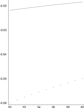
FIG. 1.: The tilt of the density perturbation spectral index $n-1$ for $d_{\perp}=6$ as a function of the number of e-foldings $N$ from the end of inflation. The solid line corresponds to the full potential of the form $1-\zeta z^{4}/{4r^{d_{\perp}-2}}$. The set of points correspond to $-3/N$, the tilt for the approximate potential $A-Cz^{4}/4$.

Let us define

$$\gamma=4\beta\left(\frac{2}{\sqrt{d_{\perp}}}\right)^{d_{\perp}+2}$$ (34)

Suppose we can approximate the potential by (32) all the way to the end of slow-roll, then

$$\eta=-3\gamma\left(\frac{z}{r_{\perp}}\right)^{2}$$ (35)

The slow-roll ends when $z_{end}=r_{\perp}/{\sqrt{3\gamma}}$. For example, if $d_{\perp}=6$, $z\sim 3.6r_{\perp}\sim 3\sqrt{d_{\perp}}r_{\perp}/2$. Therefore, before the end of slow-roll is reached (and before tachyonic instability is developed since it was assumed that $M_{S}r_{\perp}>>1$ in [20]), the approximation (32) breaks down. Moreover, since the branes almost collide at the end of inflation, there is not enough time for the branes to reheat. One should use the full inflaton potential (29).

It is useful to define $y=2z/(\sqrt{d}r_{\perp})$, so that $y_{end}<<1$ implies that the approximation (32) is valid. The slow-roll parameter $\eta$ is given by

$$\eta\sim-4\beta\left(\frac{2}{\sqrt{d_{\perp}}}\right)^{d_{\perp}}\frac{y^{2}}{\left(1-y\right)^{d_{\perp}}}\left[\left(3+\left(d_{\perp}-4\right)y\right)\left(1+\left(\frac{d_{\perp}}{4}-\frac{3}{2}\right)y\right)+y\left(1-y\right)\left(\frac{d_{\perp}}{4}-\frac{3}{2}\right)\right]$$ (36)

The slow-roll parameter $\epsilon\sim y^{6}$ and so $\epsilon<<\eta$. Hence, we will ignore it in what follows. As discussed, the velocity-dependent term has the same form as the static potential, and so its contribution to the spectral index is also negligible.

The number of e-foldings is

$$N=\frac{1}{4\beta\left(\frac{2}{\sqrt{d_{\perp}}}\right)^{d_{\perp}}}~{}\int_{y_{N}}^{y_{end}}\frac{(1-y)^{d_{\perp}-1}dy}{y^{3}\left(1+(\frac{d_{\perp}}{4}-\frac{3}{2})y\right)}$$ (37)

The tilt in the spectral index as a function of $N$ for $d_{\perp}=6$ is depicted in Figure 1. With the full potential (29), the value of $z_{end}$ at the end of slow-roll is smaller than the naive answer $r_{\perp}/\sqrt{3\gamma}$. Therefore, there is enough time to reheat, without having to invoke tachyonic instability. However, the initial condition of $z_{N}$ at $N=60$ is also smaller with the full potential. Hence the branes has to be closer to $z\sim 0$ in the beginning of inflation.

B Inverse Power Potential

A potential of the form

$$V(\phi)=\nu M_{s}^{4}\left(1-\frac{c}{\phi^{m}}\right)$$ (38)

was considered in [19, 20] when branes and anti-branes collide. The slow-roll parameters,

$$\epsilon=\frac{1}{2}M_{P}^{2}\frac{m^{2}c^{2}}{\phi^{2m+2}},\quad\quad\eta=-M_{P}^{2}\frac{m(m+1)c}{\phi^{m+2}}$$ (39)

As discussed, $m$ does not have to be $d_{\perp}-2$; for dipoles, $m=d_{\perp}-1$. Here, we can phenomenologically model the behavior of the potential with an arbitrary $c$ since its precise value depends on the brane distribution. The slow-roll condition breaks down when $\eta\sim 1$:

$$\phi_{end}\sim\left(M_{P}^{2}cm(m+1)\right)^{1/(m+2)}$$ (40)

Let us consider a velocity-dependent potential:

$$Z=1-\frac{\tilde{c}}{\phi^{m}}$$ (41)

then

$$N = -\frac{1}{M_{P}^{2}}\frac{1}{mc}\int_{\phi_{N}}^{\phi_{end}}\phi^{m+1}\left(1-\frac{\tilde{c}}{\phi^{m}}\right)d\phi$$ (42)

$$= \left(\frac{m+1}{m+2}\right)\left[\left(\frac{\phi_{N}}{\phi_{end}}\right)^{m+2}-1\right]-\frac{\tilde{c}}{\phi_{end}^{m}}\left(\frac{m+1}{2}\right)\left[\left(\frac{\phi_{N}}{\phi_{end}}\right)^{2}-1\right]$$ (43)

The solution of $\phi_{N}/\phi_{end}$ does not change greatly with the velocity-dependent term,

$$\left(\frac{\phi_{N}}{\phi_{end}}\right)^{m+2}\sim\left(\frac{m+2}{m+1}\right)N$$ (44)

Furthermore, $\epsilon<<\eta$ and so the velocity-dependent term is also negligible. Therefore,

$$n-1\sim-\frac{2}{N}\left(\frac{m+1}{m+2}\right)$$ (45)

where $m\leq d_{\perp}-2$. The spectrum is tilted to the red. If the lowest non-vanishing contribution to the potential comes from the dipole of a brane-orientifold plane system, $m=d_{\perp}-1$ which gives a slightly larger red tilt.

V Discussion

In this paper, we have examined the density perturbation spectrum in the brane inflationary scenario. We have also studied the effect of a velocity-dependent potential. The form of the inflation potential as well as the velocity-dependent potential is strongly motivated from higher dimensional gravity (in particular, string theory). In the usual four-dimensional inflationary scenario, the deviation of $Z(\phi)$ from unity is due to quantum effects and is usually small. In brane inflation, however, the velocity-dependent potential can give rise to a significant effect in $Z(\phi)$. Generically, the effect on the spectral index is comparable with that from the slow-roll parameter $\epsilon$ (from Eq.(18)). Therefore, in models where $\epsilon$ is not small, this may be a measurable effect. Even though this effect on $n$ can be small in a generic model, the scale-dependence of $n$ has a stronger dependence on the velocity dependent term, as it scales $dn/d\ln k$ by a factor of $1/Z$ (see Eq. (20)). More importantly, the velocity-dependent potential can also modify the ratio of tensor to scalar fluctuations (see Eq.(12)). With a global analysis of data from various measurements, one should be able to distinguish these effects from those that can be obtained from a conventional inflationary scenario. We expect that a few percent deviation of $Z$ from unity may be measurable.

It seems that the power spectrum index in a generic inflationary scenario in the brane world has a red tilt of a few percent. The velocity dependent potential can further tilt the density perturbation spectrum to the red or to the blue, depending on the specific form of the potential. The blue tilt due to the velocity-dependent term does not require extra fields, in contrast to other inflationary models (e.g., hybrid inflation).

The velocity-dependent potential in the brane flationary scenario is similar to that appears in k-inflation [23]. However, unlike k-inflation, in our scenario, inflation is still driven by the static potential. The additional velocity dependent term provides modifications of the usual slow-roll inflation. Furthermore, the kinetic term and the static potential in the brane inflation scenario are related by string theory or by post-Newtonian approximation (see Eq.(19)).

Potential of the type $1/\phi^{m}$ has been studied in the context of quintessence [24]. It was argued in [25] that this type of potential appear naturally in supersymmetric theory. As we have described, this type of potential is also motivated when we study cosmology involving branes. Furthermore, the velocity dependent term has a close resemblance to that in k-essence [26]. It would be interesting to explore whether the specific form of k-essence motivated by brane dynamics may offer an explanation for the present accelerating universe.

Quantum Fluctuations

In this appendix, we derive the equation for the quantum fluctuation $\delta\phi$ in the presence of a non-trivial $Z(\phi)$, and show that at late time, $\delta\phi$ and $\dot{\phi}$ obey the same differential equation with respect to time. We used this fact to derive Eq.(9) analogous to the original derivation of [11].

To study quantum fluctuations, we split $\phi$ into the classical piece $\phi_{c}$ (which satisfies (6)) and the quantum piece $\delta\phi$:

$$\phi=\phi_{c}+\delta\phi$$ (46)

The classical piece is homogeneous, whereas the fluctuations satisfy:

$$Z\left(\delta\ddot{\phi}+3H\delta\dot{\phi}\right)+Z^{\prime}\left(\ddot{\phi}+3H\dot{\phi}\right)\delta\phi-\frac{Z}{a^{2}}\nabla^{2}\delta\phi+V^{\prime\prime}\delta\phi=0$$ (47)

where we have dropped the subscript $c$ for the classical part of $\phi$. We note that for scales outside the horizon (hence the gradient term is negligible), $\delta\phi$ and $\dot{\phi}$ obeys the same time-dependent differential equation. By expanding $\delta\phi$ in fourier modes:

$$\delta\phi(x,t)=\int\frac{d^{3}k}{\sqrt{2k}}\left(a_{\bf k}\delta\phi_{\bf k}(t)e^{i{\bf k}\cdot{\bf x}}+a_{\bf k}^{\dagger}\delta\phi_{\bf k}^{*}(t)e^{-i{\bf k}\cdot{\bf x}}\right)$$ (48)

The equation of motion for $\delta\phi_{\bf k}$ is

$$Z\left(\delta\ddot{\phi}_{k}+3H\delta\dot{\phi}_{k}\right)+Z^{\prime}\left(\ddot{\phi}+3H\dot{\phi}\right)\delta\phi_{k}+\left(Z\frac{k^{2}}{a^{2}}+V^{\prime\prime}\right)\delta\phi_{k}=0$$ (49)

It is convenient to rewrite it in terms of $u_{\bf k}=a\delta\phi_{\bf k}$. In the conventional case, $Z(\phi)=1$,

$$u_{\bf k}^{\prime\prime}+\left(k^{2}-\frac{a^{\prime\prime}}{a}+a^{2}V^{\prime\prime}\right)u_{\bf k}=0$$ (50)

where prime denotes derivative with respect to conformal time $\eta=-H^{-1}e^{-Ht}$. For de Sitter space, the solution is

$$u_{\bf k}(\eta)=\frac{1}{2}\sqrt{-\pi\eta}H_{3/2}(-k\eta)$$ (51)

which reduces to $u_{\bf k}\rightarrow\frac{1}{\sqrt{2k}}e^{-ik\eta}$ for $k>>aH$ and $u_{\bf k}\sim a$ for $k<<aH$.

In the presence of a velocity-dependent potential,

$$u_{\bf k}^{\prime\prime}+\left(k^{2}-\frac{a^{\prime\prime}}{a}+\frac{a^{2}}{Z}V^{\prime\prime}-\frac{a^{2}V^{\prime}Z^{\prime}}{Z^{2}}\right)u_{\bf k}=0$$ (52)

For scales inside the horizon, when the fluctuations are generated, the dominant term is still $k^{2}$. Therefore, $u_{\bf k}$ is still given by the Bunch-Davies vacuum,

$$u_{\bf k}=\frac{1}{\sqrt{2k}}e^{-ik\eta}$$ (53)

Hence the quantum fluctuations $\delta\phi_{\bf k}$ is still given by the de Sitter temperature,

$$\delta\phi_{\bf k}=\frac{H}{2\pi}$$ (54)

REFERENCES

- [1] A. H. Guth, Phys. Rev. D 23, 347 (1981).
-
[2]
A. D. Linde,
Phys. Lett. B 108, 389 (1982);
A. Albrecht and P. J. Steinhardt, Phys. Rev. Lett. 48, 1220 (1982). -
[3]
A.T. Lee et. al. (MAXIMA-1),
astro-ph/0104459;
C.B. Netterfield et. al. (BOOMERANG), astro-ph/0104460;
C. Pryke, et. al. (DASI), astro-ph/0104490. - [4] R. Easther, B. R. Greene, W. H. Kinney and G. Shiu, hep-th/0104102.
- [5] A. Linde, Phys. Rev. D 49, 748 (1994).
-
[6]
N. Arkani-Hamed, S. Dimopoulos, G. Dvali,
Phys. Lett. B429, 263 (1998);
I. Antoniadis, N. Arkani-Hamed, S. Dimopoulos, G. Dvali, Phys. Lett. B436, 257 (1998). - [7] G. Shiu and S.-H. H. Tye, Phys. Rev. D58, 106007 (1998).
- [8] Z. Kakushadze and S.-H. H. Tye, Nucl. Phys. B548, 180 (1999).
- [9] A. Lukas, B. A. Ovrut, K. S. Stelle and D. Waldram, Phys. Rev. D 59, 086001 (1999).
- [10] G. Dvali and S.-H. H. Tye, Phys. Lett. B450, 72 (1999).
- [11] A.H. Guth, S.-Y. Pi, Phys. Rev. Lett. 49, 1110 (1982).
-
[12]
V.F. Mukhanov, G.V. Chibisov, JETP Lett. 33, 532 (1981); Sov. Phys. JETP 56, 258 (1982);
S.W. Hawking, Phys. Lett. B115, 295 (1982);
A.A. Starobinsky, ibid, B117, 175 (1982);
J. Bardeen, P.J. Steinhardt, M. Turner, Phys. Rev. D28, 679 (1983);
V.F. Mukhanov, JETP Lett. 41, 493 (1985). - [13] A.A. Starobinsky, Sov. Astr. Lett., 11, 133 (1985).
- [14] See e.g., S. Weinberg, “Gravitation and Cosmology”, Chapter 9, John Wiley & Sons, Inc., 1972.
- [15] J. Polchinski, “String Theory”, Volume II, Cambridge University Press, 1998.
-
[16]
M. Bianchi, G. Pradisi and A. Sagnotti,
Nucl. Phys. B 376, 365 (1992);
M. Bianchi, Nucl. Phys. B 528, 73 (1998) ;
Z. Kakushadze, G. Shiu and S.-H. H. Tye, Phys. Rev. D 58, 086001 (1998) ;
Z. Kakushadze, Int. J. Mod. Phys. A 15, 3113 (2000). - [17] E. Witten, JHEP 9802, 006 (1998).
-
[18]
G. Dvali, Phys. Lett. B459, 489 (1999);
N. Arkani-Hamed, S. Dimopoulos, N. Kaloper and J. March-Russell, Nucl. Phys. B 567, 189 (2000);
E.E. Flanagan, S.-H. H. Tye and I. Wasserman, Phys. Rev. D62, 024011 (2000). - [19] G. Dvali, Q. Shafi and S. Solganik, hep-th/0105203.
- [20] C. P. Burgess, M. Majumdar, D. Nolte, F. Quevedo, G. Rajesh and R. J. Zhang, hep-th/0105204.
-
[21]
S.H.S. Alexander, hep-th/0105032;
E. Halyo, hep-ph/0105341. -
[22]
C. Bachas,
Phys. Lett. B 374, 37 (1996)
;
M. R. Douglas, D. Kabat, P. Pouliot and S. H. Shenker, Nucl. Phys. B 485, 85 (1997). -
[23]
C. Armendariz-Picon, T. Damour and V. Mukhanov,
Phys. Lett. B 458, 209 (1999);
J. Garriga and V. F. Mukhanov, Phys. Lett. B 458, 219 (1999);
T. Chiba, T. Okabe and M. Yamaguchi, Phys. Rev. D 62, 023511 (2000). -
[24]
B. Ratra and P. J. Peebles,
Phys. Rev. D 37, 3406 (1988);
I. Zlatev, L. Wang and P. J. Steinhardt, Phys. Rev. Lett. 82, 896 (1999). - [25] P. Binetruy, Phys. Rev. D 60, 063502 (1999).
- [26] C. Armendariz-Picon, V. Mukhanov and P. J. Steinhardt, Phys. Rev. Lett. 85, 4438 (2000); Phys. Rev. D 63, 103510 (2001).