Magnetic susceptibility of the 2D Ising model
on a finite lattice

Abstract

Form factor representation of the correlation function of the 2D Ising model on a cylinder is generalized to the case of arbitrary disposition of correlating spins. The magnetic susceptibility on a lattice, one of whose dimensions ($N$) is finite, is calculated in both para- and ferromagnetic regions of parameters of the model. The singularity structure of the susceptibility in the complex temperature plane at finite values of $N$ and the thermodynamic limit $N\rightarrow\infty$ are discussed.

1 Introduction

The Ising model has long been a subject of great interest. The computation of the free energy [1] and spontaneous magnetization [2], Toeplitz determinant representations [3], form factor expansions [4] and nonlinear differential equations [5, 6] for the correlation functions are among the most important advances of the modern mathematical physics. The partition function of the 2D Ising model in zero field was calculated exactly [7] not only in the thermodynamic limit but also for finite lattices with different boundary conditions. The simplicity of the corresponding expressions enables one to get an idea about the mechanism of appearance of critical singularities in thermodynamic quantities from both mathematical and physical points of view.

Analytical expressions for thermodynamic quantities, which contain the dependence on lattice size, have numerous applications. For example, in computer simulation of thermodynamic systems or quantum field models one often needs such expressions to estimate the number of degrees of freedom for which a discrete numerical model is adequate to the initial continuous and infinite system. It is worth mentioning that modern experiments and technologies often deal with finite-size systems. Theoretical analysis of such systems experiences the lack of exactly solvable examples.

In this paper we present exact expressions for the 2-point correlation function and the susceptibility of the 2D Ising model on a lattice with one finite ($N={\mathrm{const}}$) and the other infinite ($M\to\infty$) dimension. These expressions are very similar to well-known form factor expansions [8], [9]. We investigate the singularity structure of the susceptibility for finite values of $N$ and discuss the thermodynamic limit $N\to\infty$.

2 Correlation function $\langle\sigma(0,0)\sigma(x,0)\rangle$

The Ising model on $M\times N$ square lattice (Fig. 1)

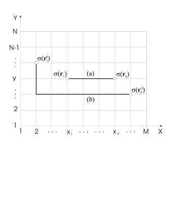
Figure 1: The numbering of the lattice sites and the variants of the disposition of correlating spins: a) along the cylinder axis, b) arbitrary disposition of spins on the lattice.

is defined by the hamiltonian $H[\sigma]$

$$H[\sigma]=-J\sum_{{\mathbf{r}}}\sigma({\mathbf{r}})(\nabla_{x}+\nabla_{y})\sigma({\mathbf{r}}),$$

where the two-dimensional vector ${\mathbf{r}}=(x,y)$ labels the lattice sites: $x=1,2,\ldots,M$, $y=1,2,\ldots,N$; the Ising spin $\sigma({\mathbf{r}})$ in each site takes on the values $\pm 1$; the parameter $J>0$ defines the energy of the coupling of adjacent spins. Shift operators $\nabla_{x}$, $\nabla_{y}$ act as follows:

$$\nabla_{x}\sigma(x,y)=\sigma(x+1,y),\quad\nabla_{y}\sigma(x,y)=\sigma(x,y+1).$$

Partition function at the temperature $\beta^{-1}$

$$Z=\sum_{[\sigma]}{\mathrm{e}}^{-\beta H[\sigma]},$$ (1)

and 2-point correlation function

$$\langle\sigma({\mathbf{r}}_{1})\sigma({\mathbf{r}}_{2})\rangle=Z^{-1}\sum_{[\sigma]}{\mathrm{e}}^{-\beta H[\sigma]}\sigma({\mathbf{r}}_{1})\sigma({\mathbf{r}}_{2})$$ (2)

are given by the sums over all possible spin configurations. It is convenient to introduce the following dimensionless parameters:

$$K=\beta J,\quad t=\tanh K,\quad s=\sinh 2K.$$ (3)

We will impose periodic boundary conditions on both axes. This gives two equations for the shift operators $\nabla_{x}$, $\nabla_{y}$:

$$(\nabla_{x})^{M}=1,\quad(\nabla_{y})^{N}=1.$$

For such boundary conditions the partition function (1) can be written as a sum of four terms [7]:

$$Z=(2\cosh^{2}K)^{MN}\cdot\frac{1}{2}\biggl{(}Q^{(f,f)}+Q^{(f,b)}+Q^{(b,f)}-Q^{(b,b)}\biggr{)}.$$ (4)

Each of them is given by the pfaffian of the operator $\widehat{D}$ (a lattice analogue of the Dirac operator)

$$Q={\mathrm{Pf\,}}\widehat{D},$$ (5)

defined by

$$\widehat{D}=\left(\begin{array}[]{cccc}0&1&1+t\nabla_{x}&1\\ -1&0&1&1+t\nabla_{y}\\ -1-t\nabla_{-x}&-1&0&1\\ -1&-1-t\nabla_{-y}&-1&0\end{array}\right).$$ (6)

The upper indices $(f,b)$ of the quantities $Q$ in (4) correspond to different types (antiperiodic or periodic) of boundary conditions for the operators $\nabla_{x},\nabla_{y}$ in (6):

$$(\nabla_{x}^{(b)})^{M}=(\nabla_{y}^{(b)})^{N}=1,\quad(\nabla_{x}^{(f)})^{M}=(\nabla_{y}^{(f)})^{N}=-1.$$ (7)

When, for example, $M\gg N$ (i.e. the torus transforms into a cylinder), then in the right hand side of (4) only the “antiperiodic” term survives:

$$Z=(2\cosh^{2}K)^{MN}Q^{(f,f)}.$$ (8)

Since the operator $\widehat{D}$ is translationally invariant, the pfaffian (5) can be easily computed. Using Fourier transformation, one finds the following factorized representation for the partition function (8):

$$Z=2^{MN}{\prod_{{\mathbf{q}}}}^{(f,f)}(s^{2}+1-s\cdot\cos q_{x}-s\cdot\cos q_{y})^{1/2}.$$ (9)

The superscript $(f)$ in the products (or sums below) implies that the quasimomentum components $q_{x}$ and $q_{y}$ run in the Brillouin zone over half-integer values in the units $2\pi/M$ and $2\pi/N$, respectively; integer values correspond to the superscript $(b)$. For example,

$${\prod_{q_{y}}}^{(f)}{\mathcal{F}}(q_{y})=\prod_{l=1}^{N}{\mathcal{F}}\biggl{(}\frac{2\pi}{N}(l+\tfrac{1}{2})\biggr{)},\qquad{\prod_{q_{y}}}^{(b)}{\mathcal{F}}(q_{y})=\prod_{l=1}^{N}{\mathcal{F}}\biggl{(}\frac{2\pi}{N}l\biggr{)}.$$

The product over one of the quasimomentum components in the right hand side of (9) can be calculated in an explicit form, so that for the partition function one has

$$Z=(2s)^{MN/2}{\prod_{q}}^{(f)}{\mathrm{e}}^{-M\gamma(q)/2}\bigl{(}1+{\mathrm{e}}^{-M\gamma(q)}\bigr{)},$$ (10)

where the function $\gamma(q)$ is the positive root of the equation

$$\sinh^{2}\frac{\gamma(q)}{2}=\sinh^{2}\frac{\mu}{2}+\sin^{2}\frac{q}{2},$$ (11)

and the parameter $\mu$ is the following function of $s$:

$$\sinh\frac{\mu}{2}=\frac{1}{\sqrt{2}}\bigl{(}\sqrt{s}-1/\sqrt{s}\bigr{)}.$$ (12)

For $q\neq 0$ $\gamma(q)$ remains positive in the whole range of the parameter $s$ ($0<s<\infty$), but $\gamma(0)$ changes its sign after crossing the critical point $s=1$. Since the product in (10) is taken over fermionic spectrum, which does not contain the value $q=0$, this does not cause any problem there. However, we will see that the ambiguity in the definition of $\gamma(0)=\pm\mu$ leads to two different representations for the correlation function.

The sum over spin configurations in the right hand side of the expression (2) for the correlation function can also be written in terms of pfaffians [10]. Corresponding matrices, however, are not translationally invariant. This fact drastically complicates the calculations. Nevertheless, the computation of the correlation function can be reduced to the computation of the determinant of a matrix

$$\langle\sigma(0)\sigma({\mathbf{r}})\rangle=\det A^{(\mathrm{dim})},$$ (13)

of considerably smaller size ${\mathrm{dim}}={\mathrm{dim}}({\mathbf{r}})$, defined by the distance between correlating spins. Further work is needed to transform the representation (13) into a representation with analytic dependence on the distance.

Form factor representation for the correlation function of the Ising model is the most acceptable from physical point of view. First it was obtained in [8] for the infinite lattice in the ferromagnetic region ($K>K_{c}$, $s>1$). Later it was extended [9] to the paramagnetic case ($K<K_{c}$, $s<1$). We note that somewhat earlier a similar representation for the 2-point Green function was deduced in [11] via $S$-matrix approach [12] for a quantum field theory model with factorized $S$-matrix ($S_{2}=-1$), which is usually associated with the scaling limit of the Ising model. The discovery of the form factor representation for the correlation function has led to the whole trend [13] in the integrable quantum field theory.

For the finite lattice the problem seems to be more difficult, but the result [14] is, in a sense, even simpler. If correlating spins are located along one of the lattice axes, the matrix in the right hand side of (13) has Toeplitz form. For example, when correlating spins are located along the horizontal axis (Fig. 1a), then

$$\langle\sigma({\mathbf{r}}_{1})\sigma({\mathbf{r}}_{2})\rangle=\det A^{(|x|)},\qquad{\mathbf{r}}_{2}-{\mathbf{r}}_{1}=(x,0),$$ (14)

and the elements of $|x|\times|x|$ matrix $A^{(|x|)}_{k,k^{\prime}}$ are given by [14]

$$A^{(|x|)}_{k,k^{\prime}}=\frac{1}{MN}{\sum_{{\mathbf{p}}}}^{(f,f)}\ \frac{{\mathrm{e}}^{ip_{x}(k-k^{\prime})}[2t(1+t^{2})-(1-t^{2})({\mathrm{e}}^{ip_{x}}+t^{2}{\mathrm{e}}^{-ip_{x}})]}{(1+t^{2})^{2}-2t(1-t^{2})(\cos p_{x}+\cos p_{y})},$$ (15)

$$\ \qquad k,k^{\prime}=0,\,1,\,\ldots,\,|x|-1.$$

As it was shown in [14] via Wiener-Hopf integral equations technique [7] adjusted to finite-size lattice, the determinant (14) can be computed analytically and for the correlation function one obtains

$$\langle\sigma{({\mathbf{r}}_{1})}\sigma{({\mathbf{r}}_{2})}\rangle = (\xi\cdot\xi_{T}){\mathrm{e}}^{-|x|/\Lambda}\sum_{l=0}^{[N/2]}g_{2l}(x),\quad\hskip 28.45274pt{\text{for\ \ }}\gamma(0)=\mu,$$ (16)

$$\langle\sigma{({\mathbf{r}}_{1})}\sigma{({\mathbf{r}}_{2})}\rangle = (\xi\cdot\xi_{T}){\mathrm{e}}^{-|x|/\Lambda}\sum_{l=0}^{[(N-1)/2]}g_{2l+1}(x),\quad{\text{for\ \ }}\gamma(0)=-\mu,$$ (17)

$$g_{n}(x) = \frac{{\mathrm{e}}^{-n/\Lambda}}{n!N^{n}}{\sum_{[q]}}^{(b)}\biggl{(}\prod_{i=1}^{n}\frac{{\mathrm{e}}^{-|x|\gamma_{i}-\eta_{i}}}{\sinh\gamma_{i}}\biggr{)}F_{n}^{2}[q],\quad g_{0}=1,$$ (18)

$$F_{n}[q] = \prod_{i<j}^{n}\frac{\sin((q_{i}-q_{j})/2)}{\sinh((\gamma_{i}+\gamma_{j})/2)},\quad F_{1}=1,$$ (19)

where $\gamma_{i}=\gamma(q_{i})$, $\eta_{i}=\eta(q_{i})$. The expressions (16), (17) are finite sums. However, the upper limits of summation can be set infinite, since it follows from (19) that the form factor $F_{n}[q]$ vanishes for $n>N$. Note an important detail — the summation over the phase volume in (18) is taken over bosonic spectrum of quasimomenta, in contrast with the initial fermionic spectrum, which determines the matrix (15). The other quantities in (16)–(19) are given by

$$\xi = |1-s^{-4}|^{1/4},$$ (20)

$$\ln\xi_{T} = \frac{N^{2}}{2\pi^{2}}\int\limits_{0}^{\pi}\frac{dp\,dq\,\gamma^{\prime}(p)\gamma^{\prime}(q)}{\sinh(N\gamma(p))\sinh(N\gamma(q))}\ln\biggl{|}\frac{\sin((p+q)/2)}{\sin((p-q)/2)}\biggr{|},$$ (21)

$$\Lambda^{-1} = \frac{1}{\pi}\int\limits_{0}^{\pi}dp\,\ln\coth({N\gamma(p)/2}),$$ (22)

$$\eta(q) = \frac{1}{\pi}\int\limits_{0}^{\pi}\frac{dp\>(\cos p-{\mathrm{e}}^{-\gamma(q)})}{\cosh\gamma(q)-\cos p}\ln\coth(N\gamma(p)/2).$$ (23)

“Cylindrical parameters” $\xi_{T}$, $\Lambda^{-1}$, $\eta(q)$ explicitly depend on the number of sites $N$ on the base of the cylinder. Their asymptotic behaviour for $N|\mu|\gg 1$ is the following:

$$\ln\xi_{T} \simeq \frac{1}{\pi}{\mathrm{e}}^{-2N|\mu|},$$ (24)

$$\Lambda^{-1} \simeq e^{-N|\mu|}\sqrt{\frac{2\sinh|\mu|}{\pi N}}$$ (25)

$$\eta(q) \simeq \frac{4{\mathrm{e}}^{-N|\mu|}}{({\mathrm{e}}^{\gamma(q)}-1)}\sqrt{\frac{\sinh|\mu|}{2\pi N}}.$$ (26)

Thus outside the critical point cylindrical parameters $\Lambda^{-1}$, $\ln\xi_{T}$ and $\eta(q)$ exponentially decrease for large $N$ and tend to zero for infinite lattice. Finite sums (16), (17) transform into series, summation over the phase volume in (18) is substituted by integration and, as a result, form factor representations on the cylinder transform into form factor representations on the infinite lattice [8], [9]. For any finite $N$ both expansions — over even $n$ (16) and over odd $n$ (17) — are valid in both ferromagnetic $(s>1)$ and paramagnetic $(s<1)$ regions. However, for $N\rightarrow\infty$, the first series is well-defined and converges in the ferromagnetic region and the second one does so in the paramagnetic region.

Recall that we started from the determinant (14) of a $|x|\times|x|$ matrix. The number of terms in its formal definition rapidly increases when $x$ grows. However, the form factor representations (16)–(19) are finite sums for any fixed $N$, and the number of terms in these sums does not depend on $|x|$. This gives a unique opportunity to verify (16)–(19) by comparing these representations with the results of transfer matrix calculations for $N$-row Ising chains. For fixed $N$ the dimension of the corresponding transfer matrix is equal to $2^{N}\times 2^{N}$. One can find analytically all eigenvectors and eigenvalues if $N$ is not too large. We have successfully performed such check analytically for $N=2,3,4$ and numerically — for $N=5,6$.

3 Correlation function $\langle\sigma(0,0)\sigma(x,y)\rangle$

The rigorous derivation of the form factor representation on the cylinder was performed in [14] only for the spins located along the cylinder axis. We have not yet succeeded in generalization of the method for arbitrary disposition of correlating spins (Fig. 1b). Meanwhile, the calculation of the momentum representation of correlation function

$$\widetilde{G}({\mathbf{p}})=\sum_{{\mathbf{r}}}{\mathrm{e}}^{i{\mathbf{p}}{\mathbf{r}}}\langle\sigma(0)\sigma({\mathbf{r}})\rangle,$$ (27)

or the susceptibility (which is related to $\widetilde{G}({\mathbf{p}}=0)$) requires an explicit dependence on both components of the vector ${\mathbf{r}}$. Form factor representations  (16)–(19) have a transparent physical content. This allows to make reasonable assumptions for corresponding generalizations. The above mentioned possibility of independent check allows to eliminate wrong hypotheses and to make correct choice. In principle, when $y$-component of the vector ${\mathbf{r}}$ is not equal to zero, all quantities in (16)–(19) could change their form. However, corresponding expressions for free bosons and fermions on the lattice prompt one of the simplest generalizations — just the substitution

$${\mathrm{e}}^{-|x|\gamma(q)}\to{\mathrm{e}}^{-|x|\gamma(q)-iyq}.$$

Suprisingly enough, this turns out to be sufficient. If instead of $g_{n}(x)$ (18) one uses the expression

$$g_{n}({\mathbf{r}})=\frac{{\mathrm{e}}^{-n/\Lambda}}{n!N^{n}}{\sum_{[q]}}^{(b)}\prod_{j=1}^{n}\left(\frac{{\mathrm{e}}^{-|x|\gamma_{j}-iyq_{j}-\eta_{j}}}{\sinh\gamma_{j}}\right)F_{n}^{2}[q],\quad g_{0}=1,$$ (28)

then the correlation functions (16) and (17) exactly coincide with the transfer matrix results for $N=2,3,4$ in the whole range of the variables $x$, $y$, $K$. Numerical calculations confirm this for $N=5,6$ as well. The validity of  (28) is out of doubts and we hope that the known answer will simplify the problem of its rigorous derivation.

As an illustration, consider the example of $N=3$. The expansions (16)–(17) are very similar to the representation of the correlation function in terms of the transfer matrix eigenvalues

$$\langle\sigma(0)\sigma({\mathbf{r}})\rangle=a_{1}(y)(\lambda_{1}/\lambda_{0})^{|x|}+a_{2}(y)(\lambda_{2}/\lambda_{0})^{|x|}+\cdots,$$ (29)

where $\lambda_{0}$ is the largest eigenvalue and the coefficients $a_{j}(y)$ are given by some bilinear combinations of the components of eigenvectors. To reduce, for example, (17) to (29), we use the following expressions for the cylindrical parameters $\xi_{T}$, $\Lambda^{-1}$, $\eta(q)$:

$$\Lambda^{-1} = \frac{1}{2}\biggl{(}{\sum_{q}}^{(f)}\gamma(q)-{\sum_{q}}^{(b)}\gamma(q)\biggr{)},$$ (30)

$${\mathrm{e}}^{-\Lambda^{-1}-\eta(q_{i})} = \frac{{\prod\limits_{q}}^{(b)}\sinh\left(\frac{\gamma(q)+\gamma(q_{i})}{2}\right)}{{\prod\limits_{q}}^{(f)}\sinh\left(\frac{\gamma(q)+\gamma(q_{i})}{2}\right)},$$ (31)

$$\xi_{T}^{4} = \frac{{\prod\limits_{q}}^{(b)}{\prod\limits_{p}}^{(f)}\sinh^{2}\left(\frac{\gamma(q)+\gamma(p)}{2}\right)}{{\prod\limits_{q}}^{(b)}{\prod\limits_{p}}^{(b)}\sinh\left(\frac{\gamma(q)+\gamma(p)}{2}\right){\prod\limits_{q}}^{(f)}{\prod\limits_{p}}^{(f)}\sinh\left(\frac{\gamma(q)+\gamma(p)}{2}\right)}.$$ (32)

One can derive these expressions from (21)–(23) by passing to contour integrals in the variable $z={\mathrm{e}}^{iq}$ and computing the residues.

For $N=3$ we have from (30)–(32) and (20)

$$\Lambda^{-1} = \frac{1}{2}\bigl{[}\gamma(\pi)+2\gamma({\pi}/{3})-\gamma(0)-2\gamma({2\pi}/{3})\bigr{]},$$ (33)

$$\xi\xi_{T} = \frac{\sinh\frac{\gamma(0)+\gamma(\pi/3)}{2}\sinh\frac{\gamma(\pi)+\gamma(2\pi/3)}{2}\sinh^{2}\frac{\gamma(2\pi/3)+\gamma(\pi/3)}{2}}{\sinh\frac{\gamma(0)+\gamma(2\pi/3)}{2}\sinh\frac{\gamma(\pi)+\gamma(\pi/3)}{2}\sinh\gamma(\pi/3)\sinh\gamma(2\pi/3)},$$ (34)

$$e^{-\Lambda^{-1}-\eta(q)} = \frac{\sinh\frac{\gamma(0)+\gamma(q)}{2}\sinh^{2}\frac{\gamma(2\pi/3)+\gamma(q)}{2}}{\sinh\frac{\gamma(\pi)+\gamma(q)}{2}\sinh^{2}\frac{\gamma(\pi/3)+\gamma(q)}{2}}.$$ (35)

Then one finds

$$\ln(\lambda_{0}/\lambda_{1}) = \Lambda^{-1}+\gamma(0),$$ (36)

$$\ln(\lambda_{0}/\lambda_{2}) = \Lambda^{-1}+\gamma(2\pi/3),$$ (37)

$$\ln(\lambda_{0}/\lambda_{3}) = \Lambda^{-1}+\gamma(0)+2\gamma(2\pi/3),$$ (38)

$$a_{1}(y) = \frac{1}{3}\frac{\sinh\frac{\gamma(0)+\gamma(2\pi/3)}{2}\sinh\frac{\gamma(\pi)+\gamma(2\pi/3)}{2}\sinh^{2}\frac{\gamma(2\pi/3)+\gamma(\pi/3)}{2}}{\sinh\frac{\gamma(0)+\gamma(\pi/3)}{2}\sinh\frac{\gamma(\pi)+\gamma(\pi/3)}{2}\sinh\gamma(\pi/3)\sinh\gamma(2\pi/3)},$$ (39)

$$a_{2}(y) = \frac{2}{3}\frac{\sinh\frac{\gamma(0)+\gamma(\pi/3)}{2}\sinh\frac{\gamma(0)+\gamma(\pi)}{2}}{\sinh\gamma(\pi/3)\sinh\frac{\gamma(\pi/3)+\gamma(\pi)}{2}}\cos(2\pi y/3),$$ (40)

$$a_{3}(y) = \frac{1}{64}\frac{1}{\sinh\frac{\gamma(0)+\gamma(\pi/3)}{2}\sinh\frac{\gamma(\pi)+\gamma(\pi/3)}{2}\sinh\frac{\gamma(0)+\gamma(2\pi/3)}{2}\sinh\frac{\gamma(\pi)+\gamma(2\pi/3)}{2}}\times$$

$$\times\frac{1}{\sinh\gamma(\pi/3)\sinh\gamma(2\pi/3)\sinh^{2}\frac{\gamma(\pi/3)+\gamma(2\pi/3)}{2}}.$$

Our $2^{3}\times 2^{3}$ transfer matrix has 8 eigenvalues, and some of them are equal. Besides that, some eigenvectors have zero components. As a result, the expression for the correlation function (29) contains only three (not seven) independent terms. If we take into account the definition (11), (12) of the function $\gamma(q)$ for particular values of quasimomentum $q=0,\ \pi/3,\ 2\pi/3,\ \pi$, we get an exact correspondence between these three terms and (36)–(3).

4 Momentum representation of the correlation
function

Since we have the expression (28) for $g_{n}({\mathbf{r}})$, which explicitly depends on both components of ${\mathbf{r}}$, we can make the Fourier transform. Let us write the momentum representation of (27) in a form similar to (16)–(17):

$$\widetilde{G}({\mathbf{p}})=\xi\xi_{T}\sum_{n}\widetilde{g}_{n}({\mathbf{p}}),$$ (42)

$$\widetilde{g}_{n}({\mathbf{p}})=\sum_{{\mathbf{r}}}{\mathrm{e}}^{-|x|/\Lambda}g_{n}({\mathbf{r}}){\mathrm{e}}^{i{\mathbf{p}}{\mathbf{r}}},$$ (43)

where

$$\sum_{{\mathbf{r}}}=\sum_{x=-\infty}^{\infty}\sum_{y=1}^{N}.$$ (44)

Performing the summation in (43), we find

$$\widetilde{g}_{n}({\mathbf{p}})=\frac{{\mathrm{e}}^{n/\Lambda}}{n!N^{n-1}}{\sum_{[q]}}^{(b)}\biggl{(}\prod_{j=1}^{n}\frac{{\mathrm{e}}^{-\eta_{j}}}{\sinh\gamma_{j}}\biggr{)}\frac{\sinh\biggl{(}\Lambda^{-1}+\sum\limits_{j=1}^{n}\gamma_{j}\biggr{)}F_{n}^{2}[q]}{\cosh\biggl{(}\Lambda^{-1}+\sum\limits_{j=1}^{n}\gamma_{j}\biggr{)}-\cos p_{x}}\delta\biggl{(}p_{y}-\sum_{j=1}^{n}q_{j}\biggr{)}.$$ (45)

The $x$-component of the quasimomentum has a continuous spectrum, $p_{x}\in[-\pi,\pi]$, but $p_{y}$ is discrete:

$$p_{y}=\frac{2\pi l}{N},\qquad l=1,\,2\,\,\ldots\,N.$$

Corresponding $\delta$-function in the right hand side of (45) has the meaning of the Kronecker symbol

$$\delta\biggl{(}p_{y}-\sum_{j=1}^{n}q_{j}\biggr{)}=\delta\biggl{(}l-\sum_{j=1}^{n}l_{j}\biggr{)}\biggm{|}_{\displaystyle{{\rm{mod}}\,N}}\,.$$

The function $\widetilde{g}_{n}({\mathbf{p}})$ is periodic in $p_{x}$, $p_{y}$ with the period $2\pi$. Inserting the “unity”

$$1=\int\limits^{\Lambda^{-1}+n\gamma(\pi)}_{\Lambda^{-1}+n\gamma(0)}d\omega\,\delta\biggl{(}\Lambda^{-1}+\sum^{n}_{j=1}\gamma_{j}-\omega\biggr{)},$$

into the sum (45) (here $\delta$ denotes Dirac $\delta$-function) and interchanging the order of summation and integration, we obtain

$$\widetilde{g}_{n}({\mathbf{p}})=\int\limits^{\Lambda^{-1}+n\gamma(\pi)}_{\Lambda^{-1}+n\gamma(0)}d\omega\frac{\sinh\omega}{\cosh\omega-\cos p_{x}}\rho_{n}(\omega,p_{y}),$$ (46)

$${\rho}_{n}(\omega,p_{y})=\frac{{\mathrm{e}}^{-n/\Lambda}}{n!N^{n-1}}{\sum_{[q]}}^{(b)}\biggl{(}\prod_{j=1}^{n}\frac{{\mathrm{e}}^{-\eta_{j}}}{\sinh\gamma_{j}}\biggr{)}F^{2}_{n}[q]\delta\biggl{(}\Lambda^{-1}+\sum_{j=1}^{n}\gamma_{j}-\omega\biggr{)}\delta\biggl{(}p_{y}-\sum_{j=1}^{n}q_{j}\biggr{)}.$$ (47)

On the infinite lattice in the scaling limit the rotational symmetry is restored and (46), (47) transform into the classical Lehmann representation in the quantum field theory.

5 Magnetic susceptibility

On $M\times N$ square lattice with equal horizontal and vertical coupling parameters the partition function $Z$ depends on four variables

$$Z=Z(K,h,N,M)=\sum_{[\sigma]}{\mathrm{e}}^{-\beta H[\sigma]+h\sum\limits_{{\mathbf{r}}}\sigma({\mathbf{r}})},$$ (48)

where dimensionless parameter $h=\beta{\mathcal{H}}$, ${\mathcal{H}}$ — magnetic field. The magnetization ${\mathfrak{M}}$ and magnetic susceptibility $\chi$ can be expressed in terms of the derivatives of the partition function with respect to $h$:

$${\mathfrak{M}}(K,h,N,M)=\frac{1}{MN}\frac{\partial\ln Z}{\partial h}=\langle\sigma\rangle,$$ (49)

$$\beta^{-1}\chi(K,h,N,M)=\frac{\partial{\mathfrak{M}}}{\partial h}=\sum_{{\mathbf{r}}}\biggl{(}\langle\sigma(0)\sigma({\mathbf{r}})\rangle-\langle\sigma\rangle^{2}\biggr{)}.$$ (50)

The magnetization for $h=0$ and finite $M$, $N$ is equal to zero due to $\mathbb{Z}_{2}$-symmetry of the Ising model. This holds even when one of the dimensions is set infinite. In the last case, when, for example, $M\to\infty$, $N={\mathrm{const}}$, 2D Ising model transforms into a 1D chain with $N$ rows, for which the spontaneous symmetry breaking is impossible. The susceptibility can be easily computed from (42)–(45)

$$\chi = \chi_{0}+\sum_{l=1}^{[N/2]}\chi_{2l}\ {\text{\hskip 65.44142pt for\ \ }}\gamma(0)=\mu,$$ (51)

$$\beta^{-1}\chi_{0} = \xi\xi_{T}N\coth(1/2\Lambda),$$ (52)

$$\chi = \sum_{l=0}^{[(N-1)/2]}\chi_{2l+1}\ {\text{\hskip 65.44142pt for\ \ }}\gamma(0)=-\mu,$$ (53)

$$\beta^{-1}\chi_{n} = \frac{{\mathrm{e}}^{-n/\Lambda}}{n!N^{n-1}}{\sum_{[q]}}^{(b)}\biggl{(}\prod_{i=1}^{n}\frac{{\mathrm{e}}^{-\eta_{i}}}{\sinh\gamma_{i}}\biggr{)}F_{n}^{2}[q]\coth\biggl{[}\frac{1}{2}\biggl{(}\Lambda^{-1}+\sum_{i=1}^{n}\gamma_{i}\biggr{)}\biggr{]}\delta\biggl{(}\sum_{i=1}^{n}q_{i}\biggr{)}.$$ (54)

In the paramagnetic region $(s<1)$ the expression (53) admits the limit $N\to\infty$ and tends to the susceptibility on the infinite lattice. However, in the ferromagnetic region $(s>1)$ one can consider the limit $N\to\infty$ only for the quantity

$$\chi_{F}=\chi-\chi_{0}=\sum_{l=1}^{\infty}\chi_{2l},$$ (55)

which reproduces well-known zero-field ferromagnetic susceptibility of the Ising model in thermodynamic limit. For large but finite $N$ the main contribution to the susceptibility is given by the term $\chi_{0}$

$$\beta^{-1}\chi_{0}\simeq 2\xi N\Lambda\simeq\frac{\sqrt{\pi}\xi N^{3/2}}{\sqrt{\sinh|\mu|}}{\mathrm{e}}^{N|\mu|},$$ (56)

which exponentially increases with the growth of the size of the cylinder base. It follows from (56) that the larger $N$ — the smaller field $\delta h\sim{\mathrm{e}}^{-N|\mu|}$ is needed to order all spins on the lattice.

Unfortunately, the exact solution for the partition function of the Ising model in external field is not known. However, the appearance of spontaneous magnetization can be deduced from the analysis of high- and low-temperature expansions. The rigorous definition of spontaneous magnetization is given by the following order of limits according to the Bogolyubov concept of quasiaverages:

$${\mathfrak{M}}_{0}(K)=\lim_{h\to 0}\bigl{[}\lim_{M,N\to\infty}{\mathfrak{M}}(K,h,N,M)\bigr{]}.$$ (57)

However, if we conjecture the decreasing of correlations at large distances and the possibility of interchanging of the corresponding limits, we can find exact solution for the squared spontaneous magnetization. It is equal to spin-spin correlation function (20) with infinite distance between correlating spins

$${\mathfrak{M}}^{2}_{0}(K)=\lim_{|{\mathbf{r}}|\to\infty}\langle\sigma(0)\sigma({\mathbf{r}})\rangle=\langle\sigma(0)\rangle\langle\sigma(\infty)\rangle=\langle\sigma\rangle^{2}=\xi.$$ (58)

Meanwhile, the sums over lattice of each summand in the right hand side of (50) do not converge in the thermodynamic limit. Therefore, the substitution of ${\mathfrak{M}}^{2}(K,0,\infty,\infty)$ by the limiting value of the correlation function (which equals $\xi$) under the (infinite) sum in the last step of the limits $h\to 0$, $M,N\to\infty$ requires not only (58), but also the existence of the limit

$$\lim_{h\to 0}\bigl{\{}\lim_{M,N\to\infty}MN\bigl{[}{\mathfrak{M}}^{2}(K,h,M,N)-\xi\bigr{]}\bigr{\}}=f(K),$$ (59)

and, moreover,

$$f(K)=0.$$ (60)

The explicit dependence of the correlation function on the size $N$, namely, the exponential tending of cylindrical parameters to their limiting values (24)–(26), can be viewed as an argument in favor of the equalities (59), (60).

The behaviour of the correlation function at large distances in the ferromagnetic region is mainly determined by the first term in the expansion (16). Note that it does not depend on $y$-projection of ${\mathbf{r}}$

$$G_{0}(|{\mathbf{r}}|)=\xi\xi_{T}{\mathrm{e}}^{-|x|/\Lambda}.$$ (61)

Therefore, the distance $\sim\Lambda$, for which spins are strongly correlated, rapidly increases (cf. with (25)) with the growth of $N$. Physically it means that for “ferromagnetic” temperatures the cylinder is divided into “domains” of size $\sim\Lambda$ with nonzero magnetization, the magnetization of the whole infinite cylinder being equal to zero. It is clear that the squared spontaneous magnetization would be more naturally defined by the value of the correlation function at large distances $|{\mathbf{r}}|=R(N)$, which do not exceed the size of the domain

$$N\ll R(N)\ll\Lambda.$$

It follows from (25) that for sufficiently large $N$ these inequalities can be satisfied. In accordance with this, the sum over $x$ with infinite limits in the definition of the thermodynamic limit of the susceptibility (50) should be substituted by a sum with the limits that do not exceed the size of the domain. In this case the condition

$$\sum_{x=-R}^{R}\sum_{y=1}^{N}[G_{0}(|{\mathbf{r}}|)-G_{0}(R)]\simeq\xi NR^{2}/\Lambda\mathop{\to}_{N\to\infty}0,$$

can be treated as a formal substantiation of the definition (55) of the susceptibility in the ferromagnetic phase. We can now estimate the “thermodynamic cutoff parameter” $R(N)$:

$$R(N)\ll\sqrt{\Lambda/N\xi}\simeq{\mathrm{e}}^{N|\mu|/2}[\pi/(2N\sinh|\mu|)]^{1/4}.$$

We believe that these estimates slightly clarify the physical content of the formal thermodynamic limit procedure.

6 Singularity structure

The initial expression (1) for the partition function of the Ising model is a polynomial in $s$, and the solution (9) is the factorized form of this polynomial. It provides an example of the mechanism of Lee-Yang “zeros” [15], which stipulates the appearance of critical singularities in the thermodynamic limit. The roots of the polynomial (9) are located on the unit circle $|s|=1$ in the complex $s$ plane. For any finite $M$ and $N$ the zero $s=1$ on the real axis does not appear, since the fermionic spectrum does not contain the value of quasimomentum $q_{x}=q_{y}=0$. When one of the dimensions increases then zeros are concentrated on the circle $|s|=1$, forming a dense set. In the limit $M\to\infty$, $N={\mathrm{const}}$ they are transformed into a finite number (equal to $N$) of the root type branchpoints, located on the circle $|s|=1$. To see this, one has to use the representation (10) and the definition (11), (12) of the function $\gamma(q)$. These branchpoints, in turn, form a dense set with the growth of $N$, but in the limit $N\to\infty$ they are transformed into four isolated logarithmic branchpoints $s=\pm 1,\,\pm i$. As a result, the specific heat in the thermodynamic limit acquires a logarithmic divergence $\sim\ln|1-s|$. It is worth noticing that the specific heat is expressed through the same function in both ferromagnetic and paramagnetic regions of $s$.

One could think that a similar picture holds for susceptibility. Indeed, the initial expression (2) for the correlation function for finite $M$ and $N$ is a ratio of polynomials in $s$. The formation of the singularities of the partition function, which stands in the denominator, we have just briefly described. Unfortunately, the polynomial in the numerator cannot be written in such simple factorized form. Nevertheless, our form factor representation for $M\to\infty$ and finite $N$ shows that the correlation function has a finite number of root branchpoints on the circle $|s|=1$. Their number is doubled in comparison with the case of partition function, since the expressions (16)–(19), (28) contain the functions $\gamma(q)$ (11), corresponding to both bosonic and fermionic values of quasimomentum. The susceptibility on the cylinder is given by the infinite sum of correlation functions and this can lead to the appearance of additional singularities. One can show, however, that these singularities do not appear on the first sheet of the appropriate Riemann surface.

As an example, let us write down the susceptibility $\chi$ (51) for $N=3$, using the expressions (39)–(3) and representations (33)–(35) for cylindrical parameters

$$\beta^{-1}\chi = \frac{\sinh\frac{\gamma(0)+\gamma(2\pi/3)}{2}\sinh\frac{\gamma(\pi)+\gamma(2\pi/3)}{2}\sinh^{2}\frac{\gamma(2\pi/3)+\gamma(\pi/3)}{2}}{\sinh\frac{\gamma(0)+\gamma(\pi/3)}{2}\sinh\frac{\gamma(\pi)+\gamma(\pi/3)}{2}\sinh\gamma(\pi/3)\sinh\gamma(2\pi/3)}\>\coth\left(\tfrac{\Lambda^{-1}+\gamma(0)}{2}\right)+$$

$$+\frac{1}{64}\frac{1}{\sinh\frac{\gamma(0)+\gamma(\pi/3)}{2}\sinh\frac{\gamma(\pi)+\gamma(\pi/3)}{2}\sinh\frac{\gamma(0)+\gamma(2\pi/3)}{2}\sinh\frac{\gamma(\pi)+\gamma(2\pi/3)}{2}}\times$$

$$\times\frac{1}{\sinh\gamma(\pi/3)\sinh\gamma(2\pi/3)\sinh^{2}\frac{\gamma(\pi/3)+\gamma(2\pi/3)}{2}}\,\coth\left(\tfrac{\Lambda^{-1}+\gamma(0)+2\gamma(2\pi/3)}{2}\right).$$

The singularities in $s$ could appear due to zero denominator in (6). It is easily seen, however, that the corresponding factors

$$\sinh\frac{\gamma(q)+\gamma(q^{\prime})}{2}=(\cos q^{\prime}-\cos q)/\sinh\frac{\gamma(q)-\gamma(q^{\prime})}{2}$$

for $q\neq q^{\prime}$ are not equal to zero. It can also be shown that on the first sheet of Riemann surface (which is determined by the condition of positivity of $\gamma(q)$, treated as functions of $s$, for real $s>0$) the arguments of cotangents in (6) also have non-zero values: these factors appear as the result of summation over coordinate $x$. Therefore, the complete set of singularities of the susceptibility is exhausted by the branchpoints contained in the functions

$${\mathrm{e}}^{\gamma(q)}=\biggl{[}\sqrt{\frac{1}{2}(s+s^{-1})+\sin^{2}\frac{q}{2}}+\sqrt{\frac{1}{2}(s+s^{-1})-\cos^{2}\frac{q}{2}}\biggr{]}^{2}$$ (63)

For each value of quasimomentum $q\neq 0,\pi$ the function (63) has four branchpoints. If we denote them by $s_{c}=|s_{c}|{\mathrm{e}}^{\pm i\varphi_{c}}$, then

$$|s_{c}|=1,\quad\cos\varphi_{c}=\left\{\begin{array}[]{r}\cos^{2}q/2\\ -\sin^{2}q/2\end{array}\right.\,.$$ (64)

It is seen from (63), that for $q=0,\pi$ there exist only two branchpoints $s_{c}=\pm i$. One can now show that for any fixed $N$ the total number of singularities is equal to $4N-2$, and all singularities are located on the unit circle $|s|=1$. We represent the corresponding picture for $N=3$ in the Fig. 2.

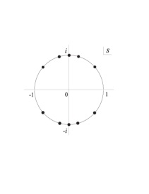
Figure 2: The location of the singularities of susceptibility $\chi$ in the complex plane $s=\sinh 2\beta J$ for $N=3$.

We do not discuss the limit $N\to\infty$, when the singularities on the circle $|s|=1$ form a dense set. This problem was seriously analyzed in [16]–[17], where the authors conjecture that the singularities form a natural boundary $|s|=1$ for the susceptibility.

We thank V. N. Shadura for his assistance in our work and helpful discussions; we are also grateful to Professor B. M. McCoy for useful comments on the form factor representation of the correlation function and for bringing the problem of singularities of the susceptibility to our attention.

This work was supported by the INTAS program under grant INTAS-00-00055.

References

- [1] L. Onsager, Crystal statistics. I. A two-dimensional model with an order-disorder transition Phys. Rev. 65, (1944), 117–149.
- [2] C. N. Yang, The spontaneous magnetization of a two-dimensional Ising model, Phys. Rev. 85, (1952), 808–816.
- [3] E. W. Montroll, R. B. Potts, and J. C. Ward, Correlations and spontaneous magnetization of the two-dimensional Ising model, J. Math. Phys. 4, (1963), 308–322.
- [4] T. T. Wu, B. M. McCoy, C. A. Tracy, and E. Barouch, Spin-spin correlation functions for the two-dimensional Ising model: Exact theory in the scaling region, Phys. Rev. B13, (1976), 316–374.
- [5] C. A. Tracy, B. M. McCoy, Neutron scattering and the correlation functions of the Ising model near , Phys. Rev. Letts. 31, (1973), 1500–1504.
- [6] M. Sato, T. Miwa, M. Jimbo, Holonomic quantum fields. IV, Publ. RIMS, Kyoto Univ. 15, (1979), 871–972.
- [7] B. M. McCoy, T. T. Wu, The Two-Dimensional Ising Model, Harvard University Press, (1973).
- [8] J. Palmer, C. A. Tracy, Two-dimensional Ising correlations: convergence of the scaling limit, Adv. Appl. Math. 2, (1981), 329–388.
- [9] K. Yamada, On the spin-spin correlation function in the Ising square lattice and the zero field susceptibility, Prog. Theor. Phys. 71, (1984), 1416–1418.
- [10] A. I. Bugrij, V. N. Shadura, Duality relation for the 2D Ising model on a finite lattice, JETP 82, (1996), 552 [Zh. Eksp. Teor. Phys. 109, (1996), 1024].
- [11] B. Berg, M. Karowski, P. Weisz, Construction of Green’s functions from an exact S matrix, Phys. Rev. D19, (1979), 2477–2479.
- [12] A. B. Zamolodchikov, Al. B. Zamolodchikov, Factorized -matrices in two dimensions as the exact solutions of certain relativistic quantum field theory models, Ann. Phys. 120, (1979), 253–291.
- [13] F. A. Smirnov, Form factors in completely integrable models of quantum field theory, Adv. Series in Math. Phys. 14, World Scientific, (1992).
- [14] A. I. Bugrij, Correlation function of the two-dimensional Ising model on the finite lattice. I, Theor. Math. Phys. 127, (2001), 528–548; hep-th/0011104.
- [15] C. N. Yang, T. D. Lee, Statistical theory of equations of state and phase transitions. I. Theory of condensation, Phys. Rev. 87, (1952), 404–409.
- [16] B. Nickel, On the singularity structure of the 2D Ising model susceptibility, J. Phys. A: Math. Gen. 32, (1999), 3889–3906.
- [17] B. Nickel, Addendum to “On the singularity structure of the 2D Ising model susceptibility”, J. Phys. A: Math. Gen. 33, (2000), 1693–1711.