Stability of ${\rm AdS}_{p}\times{\rm S}^{n}\times{\rm S}^{q-n}$ Compactifications

Abstract

We examine the stability of ${\rm AdS}_{p}\times{\rm S}^{n}\times{\rm S}^{q-n}$. The initial data constructed by De Wolfe et al [1] has been carefully analyised and we have confirmed that there is no lower bound for the total mass for $q<9$. The effective action on ${\rm AdS}_{p}$ has been derived for dilatonic compactification of the system to describe the non-linear fluctuation of the background space-time. The stability is discussed applying the positive energy theorem to the effective theory on AdS, which again shows the stability for $q\geq 9$.

]

I Introduction

Related to the bosonic M-theory[2], there is a much interest in the stability of ${\rm AdS}_{p}\times{\rm M}_{q}$ space-times with $p+q$ dimensions higher than eleven. This type of space-time appears through so-called Freund-Rubin compactifications [3] or near horizon geometry of extreme black-brane solutions. From the AdS/CFT correspondence[4] including holographic renormalisation[5] or the brane-world point of view[6], the stability of this system is a fundamental and important issue. In addition, the understanding of de Sitter (dS) space-time in string theory might be able to be accomplished by using AdS/CFT correspondence [7, 8]: How can we explain the dS entropy in the string theory? Therein our universe is assumed to be ${\rm dS}_{q}$ after Wick rotation of ${\rm S}^{q}$ of ${\rm AdS}_{p}\times{\rm S}^{q}$. In the sense of Ref [7], this means that the stability of our space-time might be related to that of the full space-time, ${\rm AdS}_{p}\times{\rm S}^{q}$, which is known to be stable.

It is well known that the full space-time will in general be unstable for ${\rm M}_{q}$ having non-trivial topology (For example, see old references [9]). This type of instability frequently happens in asymptotically flat space-times, for example, Kaluza-Klein bubble is famous one [10, 11]. The recent analysis of ${\rm AdS}_{p}\times{\rm S}^{n}\times{\rm S}^{q-n}$ shows, however, stability against linear perturbations for $q\geq 9$ [1]. They have also performed a non-linear realisation of stability in terms of the initial data [1]. Furthermore, it is shown that the energy become arbitrary negative regardless of the size of the compactified space for unstable cases ($q<9$). These discussions indicate that the instability of the higher dimensional universe, such as ${\rm dS}_{4}\times{\rm S}^{q-4}$, depends on the dimension $q$ in the sense of Ref. [7]. Here ${\rm dS}_{4}\times{\rm S}^{q-4}$ is assumed to realise as the Wick rotated ${\rm AdS}_{p}\times{\rm S}^{4}\times{\rm S}^{q-4}$ space-time.

In this paper, first of all, we reanalyse in detail the feature of the initial data presented in Ref [1] in Sec. II. We evaluate the critical dimension of the stability in several cases. Due to non-linear effects, the critical dimension might be different from that expected by the linear perturbative analysis. In Sec. III, we consider the dilatonic compactifications of ${\rm AdS}_{p}\times{\rm S}^{n}\times{\rm S}^{q-n}$ and derive the effective action on ${\rm AdS}_{p}$ to describe the non-linear effect of fluctuations, which can also describe the subsequent evolution of the initial data. Due to the curvature of the compactified space, ${\rm S}^{n}\times{\rm S}^{q-n}$, we have non-trivial effective potential for the dilatonic field. In principle, we can use the potential to justify the stability. The potential, however, does not have the lower bound. Then, we might be able to conclude that the system is always unstable, though this is not the case, since there are stable tachyonic fields in AdS [12]. In Sec. IV, we discuss this issue at the non-linear level by using the positive energy theorem for asymptotically ${\rm AdS}_{p}$ space-times. Our result shows that the system will be stable for $q\geq 9$. Finally, we give the summary in Sec. V.

II The initial data

A Freund-Rubin compactifications

We begin with the action

$$S_{p+q}=\int d^{p+q}x\sqrt{|g|}\left(\frac{1}{2}R-\frac{1}{4q!}{F_{q}}^{2}\right),$$ (1)

where $R$ is the ($p+q$)-dimensional Ricci scalar and $F_{q}$ is the field strength of the $q$-form field. The field equations are given by

$$dF_{q}=0,~{}~{}~{}d*F_{q}=0,$$ (2)

and

$$R_{MN} = \frac{1}{2(q-1)!}F_{MI_{2}\cdots I_{q}}F_{N}^{~{}~{}I_{2}\cdots I_{q}}$$ (4)

$$~{}~{}~{}-\frac{q-1}{2(p+q-2)q!}g_{MN}{F_{q}}^{2}.$$

This system admits the Freund-Rubin (FR) solution [3]. The metric of the FR solution consists of the direct sum of the $p$- and $q$-dimensional Einstein space metrics:

$$ds^{2}=g_{\mu\nu}dx^{\mu}dx^{\nu}+g_{ij}dx^{i}dx^{j},$$ (5)

where $g_{\mu\nu}$ and $g_{ij}$ are the metrics of the $p$- and $q$-dimensional Einstein spaces satisfying

$${}^{(p)}\!R_{\mu\nu}=-\frac{(p-1)}{L^{2}}g_{\mu\nu}$$ (6)

and

$${}^{(q)}\!R_{ij}=\frac{(q-1)}{R^{2}}g_{ij},$$ (7)

respectively. The field strength is given by

$$F_{q}=f*_{q}1,$$ (8)

where $f$ is a constant which is related to the curvature radii $L$ and $R$ as

$$f^{2}=\frac{2(p+q-2)(q-1)}{(p-1)R^{2}}=\frac{2(p+q-2)(p-1)}{(q-1)L^{2}},$$ (9)

and $*_{q}1$ denotes the volume form of the $q$-dimensional Einstein space.

According to the linear perturbation analysis around FR solutions [1], ${\rm AdS}_{p}\times{\rm S}^{q}$ is always stable. On the other hand, the situation changes when the $q$-dimensional space has non-trivial topology; For ${\rm AdS}_{p}\times{\rm S}^{n}\times{\rm S}^{q-n}$ with $q\geq 9$, the system is stable, while unstable for $q<9$. We shall call $q=9$ the critical dimension. It is also considered an initial data of ${\rm AdS}_{p}\times{\rm S}^{n}\times{\rm S}^{q-n}$ to demonstrate the instability of the system at non-linear level. We will describe and carefully anaylse the initial data in the next subsection.

B Time-symmetric initial data

The time-symmetric initial data considered in Ref. [1] is assumed to have the following form

$$d\ell^{2} = \frac{1}{h(r)}dr^{2}+r^{2}d\Omega_{p-2}^{2}$$ (11)

$$+e^{(q-n)\phi(r)}d\Omega_{n}^{2}+e^{-n\phi(r)}d\Omega_{q-n}^{2},$$

where

$$h(r)=1-\frac{m(r)}{r^{p-3}}+\frac{r^{2}}{L^{2}},$$ (12)

and $d\Omega_{n}^{2}$ and $d\Omega_{q-n}^{2}$ are the metrics of $S^{n}$ and $S^{q-n}$, respectively. If $\phi$ approaches zero sufficiently fast as $r\to+\infty$, the hypersurface is expected to be asymptotically ${\rm AdS}_{p}\times{\rm S}^{n}\times{\rm S}^{q-n}$.

Since we are considering the time-symmetric initial data, the equation to be solved is just the Hamiltonian constraint

$$(p-2)\frac{m^{\prime}(r)}{r^{p-2}} = \frac{1}{4}qn(q-n)h(r)\phi^{\prime 2}-\frac{q-1}{R^{2}}\left[ne^{-(q-n)\phi(r)}\right.$$ (14)

$$\left.~{}~{}~{}+(q-n)e^{n\phi(r)}-q\right].$$

The momentum constraint is automatically satisfied.

We set $\phi(r)=\phi_{0}e^{-r/a}$ $(\phi_{0}={\rm constant})$ and numerically solve the equation for $m(r)$ with the regular boundary condition at the center, $m(r\sim 0)=O(r^{\lambda})$, where $\lambda\geq p-1$. This regularity condition is important when one argues the positivity of the total mass (c.f. Schwarzschild solution with $M<0$). For convenience’ sake, we introduce dimensionless variables:

$$\ell:=L/a,~{}~{}\rho:=r/a,~{}~{}y:=m/L^{p-3}.$$ (15)

Then, Eq. (14) becomes

$$(p-2)\frac{\ell^{p-3}}{\rho^{p-2}}y^{\prime}(\rho)=\frac{qn(q-n)}{4}\left[1-\frac{\ell^{p-3}}{\rho^{p-3}}y(\rho)+\frac{\rho^{2}}{\ell^{2}}\right]\phi^{2}$$ (16)

$$-\frac{(p-1)^{2}}{\ell^{2}(q-1)}\left[ne^{-(q-n)\phi}+(q-n)e^{n\phi}-q\right].$$ (17)

This system is characterized by five parameters $\{p,q,n,\ell,\phi_{0}\}$. Typical behavior of the mass function $y(\rho)$ is shown in Fig. 1. We have computed the asymptotic values of the mass function $y_{\infty}:=\lim_{\rho\rightarrow+\infty}y(\rho)$ for a sufficiently wide range of parameters, and confirmed that a negative mass solution can arise only when $q<9$. The tables I-IV shows this critical dimension $q=9$. We can see from these tables that a negative mass solution likely arises when (i) $p$ is small, (ii) $q$ is small, and (iii) $n$ is close to $q/2$. For $\ell\ll 1$, Eq. (17) takes the form

$$y^{\prime}\simeq\varphi(p,q,n,\phi_{0},\rho)\ell^{-p+1},$$ (18)

which implies that $y_{\infty}\propto\ell^{-p+1}$ for fixed values of the other parameters. Hence if we find a negative mass solution for $\ell\ll 1$, then we can also obtain solutions with arbitrarily large negative mass, which indicates the instability of the system.

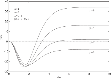
FIG. 1.: The mass function $y(\rho)$ with parameters $p=6,7,8,9$, $q=4$, $n=2$, $\ell=0.1$, $\phi_{0}=0.1$.

Here we must have a minor comment on the evaluation of the critical dimension. For $\phi\ll 1$, Eq. (14) becomes

$$\frac{p-2}{qn(q-n)}\frac{m^{\prime}(r)}{r^{p-2}}\simeq h(r)\phi^{\prime 2}-2\frac{(p-1)^{2}}{L^{2}(q-1)}\phi^{2}.$$ (19)

In Ref. [1] there is a rough argument to evaluate the critical dimension by assuming the positive signature of $m(r)$ in $h(r)$ in the right-hand side. However, $m(r)$ does not have a definite signature.

III Effective theory on AdS

From now on we derive the effective theory which describes the time evolution of the initial data presented in the previous section. To do so, we consider only zero-modes. Since we are interested in the dynamics of the full space-time, we adopt the following standard dimensional reduction:

$$ds^{2}=g_{\mu\nu}(x)dx^{\mu}dx^{\nu}+e^{2\phi_{1}(x)}d\Omega_{n}^{2}+e^{2\phi_{2}(x)}d\Omega_{q-n}^{2}.$$ (20)

The curvature radii of $S^{n}$ and $S^{q-n}$ are normalized such that Eq. (20) gives the Freund-Rubin metric when $\phi_{1}=\phi_{2}=0$. Then, the following form of the $q$-form field

$$F_{q}=f*_{n}1\wedge*_{q-n}1,$$ (21)

where $*_{n}1$ and $*_{q-n}1$ are the volume forms of $S^{n}$ and $S^{q-n}$, respectively, solves the field equations (2). Then, the Einstein equation becomes

$${}^{(p)}\!R_{\mu\nu} = -\frac{(p-1)}{L^{2}}e^{-2\psi}g_{\mu\nu}+\nabla_{\mu}\nabla_{\nu}\psi$$ (23)

$$+n\nabla_{\mu}\phi_{1}\nabla_{\nu}\phi_{1}+(q-n)\nabla_{\mu}\phi_{2}\nabla_{\nu}\phi_{2},$$

and

$$\nabla^{2}\Phi^{X}+\nabla_{\mu}\psi\nabla^{\mu}\Phi^{X}=\frac{(q-1)}{R^{2}}(e^{-2\Phi^{X}}-e^{-2\psi}),$$ (24)

where $\nabla$ denotes the covariant derivative with respect to $g_{\mu\nu}$, $\Phi^{X}$ represents $\phi_{1}$ and $\phi_{2}$, and

$$\psi:=n\phi_{1}+(q-n)\phi_{2}$$ (25)

has been defined. To eliminate terms including second derivative of $\psi$ in Eq. (23), we perform the conformal transformation:

$$g_{\mu\nu}\mapsto\bar{g}_{\mu\nu}=e^{2\psi/(p-2)}g_{\mu\nu}$$ (26)

Then, Eqs. (23), (24) become

$${}^{(p)}\!\bar{R}_{\mu\nu} = \frac{n(p+n-2)}{p-2}\bar{\nabla}_{\mu}\phi_{1}\bar{\nabla}_{\nu}\phi_{1}$$ (27)

$$+ \frac{2n(q-n)}{p-2}\bar{\nabla}_{(\mu}\phi_{1}\bar{\nabla}_{\nu)}\phi_{2}$$ (28)

$$+ \frac{(q-n)(p+q-n-2)}{p-2}\bar{\nabla}_{\mu}\phi_{2}\bar{\nabla}_{\nu}\phi_{2}$$ (29)

$$+ \frac{f^{2}}{2(p-2)}\biggl{\{}e^{-\frac{2(p-1)}{p-2}\psi}$$ (31)

$$-\frac{(p-1)[ne^{-2\phi_{1}}+(q-n)e^{-2\phi_{2}}]}{(p+q-2)}e^{-\frac{2}{p-2}\psi}\biggr{\}}\bar{g}_{\mu\nu},$$

$$\bar{\nabla}^{2}\Phi^{X}+\frac{f^{2}(p-1)}{2(p+q-2)}\left\{e^{-\frac{2(p-1)}{p-2}\psi}\right.\left.-e^{-2\Phi^{X}}e^{-\frac{2}{p-2}\psi}\right\}=0.$$ (33)

These are derived by variation of the effective action in Einstein frame:

$$\bar{S}=\int d^{p}x\sqrt{|\bar{g}|}\left[\frac{1}{2}{}^{(p)}\!\bar{R}-\frac{1}{2}G_{XY}\bar{g}^{\mu\nu}{\Phi^{X}}_{\!\!,\mu}{\Phi^{Y}}_{\!\!,\nu}-V(\Phi)\right],$$ (34)

where

$$G = \frac{n(p+n-2)}{p-2}d{\phi_{1}}^{\!\!2}+\frac{2n(q-n)}{p-2}d\phi_{1}d\phi_{2}$$ (36)

$$+\frac{(q-n)(p+q-n-2)}{p-2}d{\phi_{2}}^{\!\!2}$$

and

$$V(\Phi) = \frac{f^{2}}{4}e^{-\frac{2(p-1)}{p-2}\psi}-\frac{f^{2}(p-1)}{4(p+q-2)}$$ (38)

$$\times[ne^{-2\phi_{1}}+(q-n)e^{-2\phi_{2}}]e^{-\frac{2}{p-2}\psi}.$$

Unstable modes in Ref. [1] corresponds to the $\psi=0$ case with the potential

$$V(\Phi) = \frac{f^{2}}{4}\left\{1-\frac{p-1}{4(p+q-2)}\right.$$ (40)

$$\times\left[ne^{-2\phi_{1}}+(q-n)e^{\frac{2(q-n)}{n}\phi_{1}}\right]\biggr{\}}$$

For ${\rm AdS}_{p}\times{\rm S}^{q}$ the potential can be obtained by setting $n=q$ and $\phi_{2}=0$ ($\psi=q\phi_{1}$);

$$V(\Phi)=\frac{f^{2}}{4}\left[e^{-\frac{2q(p-1)}{p-2}\phi_{1}}-\frac{q(p-1)}{p+q-2}e^{-\frac{2(p+q-2)}{p-2}\phi_{1}}\right].$$ (41)

This has the lower bound $V(0)=-(p-1)(p-2)/2L^{2}$ at $\phi_{1}=0$ and the system is definitely stable (See Fig. 2).

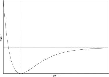
FIG. 2.: This is the typical profile of the potential $V(\Phi)$ for ${\rm AdS}_{p}\times{\rm S}^{q}$. It is definitely stable.

At first glance, the system seems to be unstable because the potential (38) does not have the lower bound. However, we must carefully analyse the stability because we are thinking of the asymptotically AdS space-times, in which case a tachyonic field may be stable [12]. Correspondingly, the system can be stable if the potential satisfies a certain condition [13].

IV Implications from the positive energy theorem

In this section, we discuss the stability of the ${\rm AdS}_{p}\times{\rm S}^{n}\times{\rm S}^{q-n}$ space-time by applying the positive energy theorem [13, 14] to the effective theory on ${\rm AdS}_{p}$.

If the scalar potential can be written in the form

$$V=2(p-2)^{2}G^{XY}\frac{\delta W}{\delta\Phi^{X}}\frac{\delta W}{\delta\Phi^{Y}}-2(p-1)(p-2)W^{2},$$ (42)

we can show the positivity of the total energy in the Einstein frame [13]. Indeed, the total energy can be expressed as

$$M_{\rm AD}=\int_{\Sigma}d^{p-1}x\biggl{[}2|\hat{D}\epsilon|^{2}+\sum_{X}|\delta\lambda^{(X)}|^{2}\biggr{]},$$ (43)

where $\Sigma$ is the asymptotically ${\rm AdS}_{p}$ space-like hypersurface, $\hat{D}_{\mu}:=D_{\mu}+iW(\Phi)\gamma_{\mu}$ with the spinor covariant derivative $D_{\mu}$, and $\epsilon$ is the spinor satisfying the Witten equation, $\sum_{a=1}^{p-1}\gamma^{a}\hat{D}_{a}\epsilon=0$. The spinor $\delta\lambda^{(X)}$ is defined by

$$\delta\lambda^{(X)}=\frac{1}{\sqrt{2}}\left[if^{(X)}_{Y}\gamma^{\mu}\partial_{\mu}\Phi^{Y}+2(p-2)f^{(X)Y}\frac{\delta W}{\delta\Phi^{Y}}\right]\epsilon,$$ (44)

where $f^{(X)}_{Y}$ is such that

$$G_{XY}=\sum_{Z}f^{(Z)}_{X}f^{(Z)}_{Y}$$ (45)

holds, which can be thought of as the orthonormal basis of the target space.

For simplicity, we consider the situation in which the effective theory is described by a single scalar field $\Phi$ defined by

$$\phi_{1}=\frac{\alpha}{n}\Phi,~{}~{}~{}\phi_{2}=\frac{\beta}{q-n}\Phi.$$ (46)

By the scaling property of the scalar field, we can put

$$\alpha+i\beta=e^{i\theta},~{}~{}~{}(0\leq\theta<\pi),$$ (47)

without loss of generality. This contains both of the typical stable and unstable systems. The parameter adopted in Sec. IIB corresponds to $\alpha=-\beta$, $(\theta=3\pi/4)$. The target space metric and the effective potential become

$$G = \left[\frac{(\alpha+\beta)^{2}}{p-2}+\frac{\alpha^{2}}{n}+\frac{\beta^{2}}{q-n}\right]d\Phi^{2}$$ (48)

and

$$V(\Phi) = \frac{f^{2}}{4}e^{-\frac{2(p-1)(\alpha+\beta)}{p-2}\Phi}$$ (51)

$$-\frac{f^{2}(p-1)}{4(p+q-2)}[ne^{-2\alpha\Phi/n}+(q-n)e^{-2\beta\Phi/(q-n)}]$$

$$\times e^{-\frac{2(\alpha+\beta)}{p-2}\Phi}.$$

The asymptotically AdS condition requires that the scalar field approaches $\Phi=0$ at spatial infinity, where the effective potential has a stationary point. To confirm whether there exist a functional $W(\Phi)$ satisfying Eq. (42), we expand the effective potential in terms of $\Phi$ under the assumption $|\Phi|\ll 1$. Up to the second order in $\Phi$, the effective potential becomes

$$V(\Phi)=V_{0}+V_{1}\Phi+\frac{1}{2}V_{2}\Phi^{2}+O(|\Phi|^{3}),$$ (52)

where

$$V_{0} = -\frac{f^{2}(p-2)(q-1)}{4(p+q-2)},$$ (53)

$$V_{1} = 0,$$ (54)

$$V_{2} = \frac{f^{2}(p-1)}{(p+q-2)}$$ (56)

$$\times\left[\frac{(\alpha+\beta)^{2}(p+q-3)}{p-2}-\frac{\alpha^{2}}{n}-\frac{\beta^{2}}{q-n}\right].$$

The functional $W(\Phi)$ is also expanded as

$$W(\Phi)=W_{0}+W_{1}\Phi+\frac{1}{2}W_{2}\Phi^{2}+O(|\Phi|^{3}).$$ (57)

From Eq. (42) we find

$$W_{0} = \pm\frac{f}{2}\sqrt{\frac{q-1}{2(p-1)(p+q-2)}},$$ (58)

$$W_{1} = 0,$$ (59)

and $W_{2}$ is determined by solving the following algebraic equation:

$$G^{\Phi\Phi}{W_{2}}^{2}-\frac{W_{0}(p-1)}{p-2}W_{2}-\frac{1}{4(p-2)^{2}}V_{2}=0,$$ (60)

which has real solutions if

$$\frac{(\alpha+\beta)^{2}(8p+9q-25)}{p-2}+\left(\frac{\alpha^{2}}{n}+\frac{\beta^{2}}{q-n}\right)(q-9)\geq 0$$ (61)

is satisfied. The condition that the above inequality holds for every values of $\alpha$, $\beta$ is

$$\frac{(p+q-2)(q-9)(q-1)}{n(q-n)(p-2)}\geq 0.$$ (62)

This means that the total energy is always positive for small fluctuation of $\Phi$ if $q\geq 9$ is satisfied, which is consistent with the linear analysis in Ref. [1]. When $q=9$, a double real root appears for $\theta=3\pi/4$, of which direction the potential $V$ shows negative mass squared.

FIG. 3.: (a) The functional $W$ and (b) the potential $V$ of the scalar field with the parameter $(p,q,n)=(4,10,4)$ and $\theta=0$ (solid line), $\pi/4$ (dashed line), $\pi/2$ (dotted line), $3\pi/4$ (dot-dashed line). Even if the potential shows negative mass squared when $\theta=3\pi/4$, we can find $W$.

For large fluctuations of $\Phi$, we need numerical calculations to confirm the existence of the functional $W(\Phi)$. This seems to be almost promising work, because we can have the asymptotic solutions of $W(\Phi)$ at $\Phi\to\pm\infty$ and all the higher order terms for $|\Phi|\ll 1$ as Eq. (57). The numerical analysis shows that there is always the functional $W(\Phi)$ when $q\geq 9$. Some cases are shown in Fig. 3.

Thus, we expect that the ${\rm AdS}_{p}\times{\rm S}^{n}\times{\rm S}^{q-n}$ for $q\geq 9$ is stable even for large fluctuations. The advantages of the use of the positive energy theorem are (i) one can confirm stability of the background geometry beyond linear perturbative analysis, (ii) one can argue the semi-classical or quantum mechanical stability without topology change of the space-time, and (iii) the background geometry need not be exactly ${\rm AdS}_{p}\times{\rm S}^{n}\times{\rm S}^{q-n}$; the positive energy theorem can be applied to the case of the non-trivial spatial topology such as black hole space-times [17].

V Summary

In this paper we examined the stability of ${\rm AdS}_{p}\times{\rm S}^{n}\times{\rm S}^{q-n}$, that is, generalised Freund-Rubin compactifications. We confirmed that there are initial data having the arbitrary negative total mass for $q<9$.

We have constructed the effective theory on AdS and then considered the condition that the positivity of the total mass can be confirmed. We can expect that the ${\rm AdS}_{p}\times{\rm S}^{n}\times{\rm S}^{q-n}$ for $q\geq 9$ is also stable under quantum mechanical or non-linear fluctuations. Furthermore, this argument will also hold for AdS-black hole background, which might be relevant for the stability of some thermal ${\rm CFT}_{p-1}$ according to the AdS/CFT correspondence.

We are interested in the time evolution of the initial data with the negative energy. In the case of Kaluza-Klein bubble with the negative energy, it is remembered that we can see the tendency of the appearance of the naked singularity, although we cannot have the definite answer since this relies on numerical analysis [19]. Similarly, such a problem for the present situation will be also shared. We need systematic and numerical analysis to clarify this point.

$q\backslash n$	$2$	$3$	$4$
4	4	*	*
5	5	*	*
6	5	5	*
7	7	6	*
8	11	10	9
9	+	+	+

TABLE I.: $\ell=0.01$, $\phi_{0}=1$ case. The figures displayed denote the maximum dimension $p$ for the negative mass. $+$ means that the mass is positive. $*$ denotes redundant cases.

$q\backslash n$	$2$	$3$	$4$
4	4	*	*
5	4	*	*
6	5	5	*
7	7	6	*
8	11	10	9
9	+	+	+

TABLE II.: $\ell=0.1$, $\phi_{0}=1$.

$q\backslash n$	$2$	$3$	$4$
4	4	*	*
5	5	*	*
6	6	6	*
7	8	8	*
8	12	12	11
9	+	+	+

TABLE III.: $\ell=1$, $\phi_{0}=1$.

$q\backslash n$	$2$	$3$	$4$
4	4	*	*
5	4	*	*
6	4	4	*
7	5	5	*
8	9	9	9
9	+	+	+

TABLE IV.: $\ell=0.01$, $\phi_{0}=0.01$.

REFERENCES

• [1] O. DeWolfe, D. Z. Freedman, S. S. Gubser, G. T. Horowitz and I. Mitra, hep-th/0105047.
• [2] G. T. Horowitz and L. Susskind, hep-th/0012037.
• [3] P. G. O. Freund and M. A. Rubin, Phys. Lett. 97B, 233(1980).
• [4] J. Maldacena, Adv. Theor. Math. Phys., 2, 231(1998); O. Aharony, S. S. Gubser, J. Maldacena, H. Ooguri and Y. Oz, Phys. Rep. 323, 183(2000).
• [5] J. de Boer, E. Verlinde and H. Verlinde, JHEP 0008, 003(2000).
• [6] L.Β Randall and R.Β Sundrum, Phys. Rev. Lett. 83, 3370(1999); 83, 4690(1999).
• [7] V. Balasubramanian, P. HoΕ™ava and D. Minic, JHEP 0105,043(2001).
• [8] A. Strominger, hep-th/0106113.
• [9] K. Ito and O. Yasuda, Phys. Rev. Lett. 52, 1849(1984); O. Yasuda, Nucl. Phys. B246, 170(1984).
• [10] E. Witten, Nucl. Phys. B195, 481(1982).
• [11] D. Brill and G. T. Horowitz, Phys. Lett. B262, 437(1991).
• [12] P. Breitenlohner and D. Z. Freedman, Phys. Lett. B115, 197(1982).
• [13] P. K. Townsend, Phys. Lett. 148B, 55(1984).
• [14] R. Schoen and S. T. Yau, Commun. Math. Phys. 79, 23(1981); E. Witten, Commun. Math. Phys. 80, 381(1981); J. M. Nester, Phys. Lett. 83A, 241(1981).
• [15] L. F. Abbott and S. Deser, Nucl. Phys. B195, 76(1982).
• [16] A.Β Ashtekar and A.Β Magnon, Class. Quantum Grav. 1, L39(1984); A.Β Ashtekar and S.Β Das, Class. Quantum. Grav. 17, L17(2000).
• [17] G. W. Gibbons, S. W. Hawking, G. T. Horowitz and M. J. Perry, Commun. Math. Phys. 88, 295(1983)
• [18] G. W. Gibbons, C. M. Hull and N. P. Warner, Nucl. Phys. B218, 173(1983).
• [19] S. Corley and T. Jacobson, Phys. Rev. D49, 6261(1994); H. Shinkai and T. Shiromizu, Phys. Rev. D62, 024010(2000).
Β