We study D-branes on Calabi-Yau manifolds, carrying charges which are torsion elements of the K-theory. Interesting physics ensues when we follow these branes into nongeometrical phases of the compactification. On the level of K-theory, we determine the monodromies of the group of charges as we circle singular loci in the closed string moduli space. Going beyond K-theory, we discuss the stability of torsion D-branes as a function of the Kähler moduli. When the fundamental group of the Calabi-Yau is nonabelian, we find evidence for new threshold bound states of BPS branes. In a two-parameter example, we compare our results with computations in the Gepner model. Our study of the torsion D-branes in the compactification of [1] sheds light on the physics of that model. In particular, we develop a proposal for the group of allowed D-brane charges in the presence of discrete RR fluxes.

Return of the Torsion D-Branes

1 Introduction

It is by now well established that D-brane charges are classified by K-theory. More precisely, for branes on a Calabi-Yau, the even dimensional holomorphic branes are determined by $K^{0}$ theory, whereas the charges of the branes wrapping middle dimensional special Lagrangian cycles are given by $K^{1}$. As one moves around in the closed string moduli space, the group of charges is expected to vary. In particular, if one traverses non-contractible loops in the bulk moduli space, the group of charges comes back only up to an automorphism. K-theory provides a natural framework to study such monodromies, since those act within $K^{0}$ and within $K^{1}$. Monodromy actions on the free part of K-theory $K^{0}/K^{0}_{tor}$ ( or $K^{1}/K^{1}_{tor}$) have been studied using mirror symmetry. Restricting to the free part of K-theory, it was sufficient to study the dependence of $K^{0}/K^{0}_{tor}$ on the Kähler moduli and $K^{1}/K^{1}_{tor}$ on complex structure moduli.

The investigation of the dependence of the torsion part of K-theory on the bulk moduli was started in [2]. There, examples were presented in which the monodromies acted trivially on the torsion subgroup $K^{\bullet}_{tor}$. As predicted in [2] this is not the case in general, as will be shown in this paper in examples. It turns out that both $K^{0}_{tor}$ and $K^{1}_{tor}$ undergo monodromy as we vary the Kähler moduli. Since the monodromies act nontrivially on the torsion subgroup, it follows that they act nontrivially also on the full K-theory. Similarly, we will find that $K^{0}$ undergoes nontrivial automorphisms in the complex structure moduli space.

In addition to D-brane charge, K-theory also classifies the fluxes of the RR-fields. The presence of torsion classes in K-theory allows one to turn on discrete RR-fluxes. As a result, one might expect that the full moduli space of a theory has several branches, corresponding to turning on different fluxes. In [3] it was shown that such fluxes can alter the spectrum of allowed D-brane charges. We will see an example of such a phenomenon, though our criterion for which fluxes survive is different from theirs.

In general, one is also interested in the physics of D-branes beyond K-theory, such as moduli spaces, brane dynamics and stability. In section 3 we start the investigation of the physics of torsion D-branes, discussing the stability of brane configuration carrying torsion charge at various points in moduli space. Since these questions depend on Kähler moduli, we cannot use large volume concepts everywhere, but have to employ other techniques, such as boundary conformal field theory, to get information about the stringy regime.

We then move on to discuss three different examples, each of which is suitable to highlight certain features of torsion D-branes. In §4, we study one of the very few examples of a Calabi-Yau with a non-abelian fundamental group. This example motivates a conjecture for the general form of the monodromy about (the mirror of) the conifold locus, which generalizes a previous conjecture which – we now see – holds when the Calabi-Yau is simply-connected.

In [2], we found that, when the Calabi-Yau, $X$, is not simply-connected, there are stable BPS branes carrying 6-brane charge. These are distinguished from the usual wrapped 6-brane by a discrete conserved charge – a torsion element in K-theory. These branes were associated to one-dimensional irreps of the fundamental group of $X$. In the example if §4, we also “discover” the existence of stable BPS branes corresponding to higher dimensional irreps of the fundamental group. In contrast to the previous case, these are not distinguished by any conserved (discrete) charge from a collection of wrapped 6-branes. Nonetheless, we argue that they must be present as threshold bound states in the multiple 6-brane system in order to account for the monodromies that we find.

The second example, discussed in §5, is a model whose Kähler moduli space has complex dimension 2. As usual in studying such two-parameter models, the structure of the Kähler moduli space is rather more complicated than in the one-parameter case, and it is interesting to see that one can produce a consistent set of monodromies acting on the K-theory. We do have an advantage in this case; the moduli space contains a Gepner point. So we can compare the results of our topological calculations with the results from CFT.

The first two examples are two more examples where the monodromies act trivially on the torsion subgroup of the K-theory. The third example, discussed in §6 is a free $\BZ_{2}$ orbifold of $K3\times T^{2}$. This manifold played a major role in the context of heterotic-IIA duality, and D-branes on it were discussed in [4, 5]. It was shown in [1] that IIA theory on this manifold, with a discrete RR Wilson line turned on, has a heterotic dual.

This manifold introduces several new features. Unlike previous cases, the torsion in $K^{0}(X)$ is not captured by the flat line bundles on $X$. Second (and related) is the possibility of turning on a flat, but topologically nontrivial $H$-field, which leads to D-brane charge taking values in the twisted K-theory (which we also compute). Third, the monodromies do act nontrivially on the torsion subgroups.

The effect of turning on discrete RR flux is nontrivial. First of all, it changes the global structure of the moduli space (the moduli space is a finite cover of the moduli space without the RR flux). Second, it restricts the spectrum of allowed D-branes. In §6.3, we make a proposal for the precise form of this restriction. In §6.4, we investigate the physics near various singular loci in the moduli space. In particular, we see that our proposed restriction on D-brane charges in the presence of discrete RR flux is precisely what is required to make sense of the physics near the singularity. This “explains” from the Type IIA perspective why it was necessary to turn on the discrete flux.

2 Review

In this section, we collect some of the results of [2] which will be useful for our present investigations.

Every Calabi-Yau manifold, $X$, whose holonomy group is $SU(3)$, has a finite fundamental group, and is the quotient of a simply-connected Calabi-Yau, $Y$ by a finite group, $G$, of freely-acting holomorphic automorphisms (which preserve the holomorphic 3-form). The most familiar constructions of Calabi-Yau manifolds – as hypersurfaces or complete intersections in toric varieties – yield simply-connected Calabi-Yau manifolds, which are candidates for the covering space, $Y$. The K-theory of such a $Y$ is torsion-free. So, to find a suitable Calabi-Yau manifold, $X$, with torsion in its K-theory, we look for a freely-acting group $G$ to mod out by.

The first problem is to compute the K-theory of $X=Y/G$. For this, we used a pair of spectral sequences, the Cartan-Leray Spectral Sequence – which computes the homology of $X$ from the homology of $Y$ – and the Atiyah-Hirzebruch Spectral sequence, which computes the K-theory of $X$ from the cohomology of $X$. Some very useful discussions of the AHSS have appeared in the recent physics literature [2, 6, 7, 8].

For a Calabi-Yau manifold (indeed, for a 6-manifold with $H^{1}(X)=0$), the AHSS converges at the $E_{2}$ term,

$$E_{2}^{p,q}=\coho{p}{X,\pi_{q}(BU)}$$ (2.1)

where $\pi_{2n}(BU)=\BZ$, $\pi_{2n+1}(BU)=0$. And, after a bit of computation, one finds that the torsion subgroups of the K-theory (our main interest) fit into exact sequences

$$0\to\coho{4}{X}_{tor}\to K^{0}(X)_{tor}\to\coho{2}{X}_{tor}\to 0$$ (2.2)

$$0\to\coho{5}{X}\to K^{1}(X)_{tor}\to\coho{3}{X}_{tor}\to 0$$ (2.3)

(note that 5X is pure torsion).

The Universal Coefficients Theorem and Poincaré duality determine

$$\coho{5}{X}_{tor}=\homo{1}{X}_{tor}=(\coho{2}{X}_{tor})$$

$$\coho{4}{X}_{tor}=\homo{2}{X}_{tor}=(\coho{3}{X}_{tor})^{*}$$ (2.4)

and the homology groups can be determined from the CLSS, a homology spectral sequence with $E^{2}$ term

$$E^{2}_{p,q}=\homo{p}{G,\CH_{q}(Y)}$$ (2.5)

the homology with twisted coefficients.

Define the coinvariant quotient, $\homo{2}{Y}_{G}=\homo{q}{Y}/\CA$, where $\CA$ is the subgroup of $\homo{2}{Y}$ generated by elements of the form $x-g\cdot x$. Assuming that $\homo{2}{Y}_{G}$ is torsion-free, we find the needed homology groups to be given by

$$\homo{1}{X}=\homo{1}{G}=G/[G,G]$$ (2.6)

and the exact sequence

$$0\to\homo{2}{Y}_{G}\xrightarrow{\pi_{*}}\homo{2}{X}\to\homo{2}{G}\to 0$$ (2.7)

where $\pi_{*}$ is the push-forward by the projection $\pi:Y\to X$. With this, the K-theory of the various examples can be calculated.

One notational point. We will frequently be interested in the class in $K^{0}(X)$ corresponding to a D-brane wrapped on a (holomorphic) submanifold $Y\stackrel{{\scriptstyle i}}{{\hookrightarrow}}X$. This class is the push-forward in K-theory and should probably be written as $i_{!}\CO_{Y}$. We will abbreviate this as $\CO_{Y}$. Some readers will note that this is the same notation used for a certain coherent sheaf on $X$ – the structure sheaf of $Y$. We hope that any confusion that arises because of this similarity in notation will prove to be beneficial.

As we move away from large-radius, into the interior of the moduli space, the group of D-brane charges is no longer given by topological K-theory. Still, as a discrete abelian group, it is locally constant. When we traverse some incontractible cycle in the moduli space (circle some singular locus), the group of D-brane charges comes back to itself up to an automorphism.

These monodromies must satisfy the following properties

• They descend to the known action on on $K^{\bullet}(X)/K^{\bullet}(X)_{tor}$, which can be computed, say, using Mirror Symmetry.

• They preserve the skew-symmetric intersection pairing

  $$(.,.):K^{0}(X)\times K^{0}(X)\to\BZ$$

  given by

  $$\begin{split}(v,w)&=Ind(\overline{\partial}_{v\otimes\overline{w}})\\ &=\int_{X}ch(v\otimes\overline{w})Td(X)\end{split}$$ (2.8)

  which annihilates $K^{0}_{tor}(X)$ and is nondegenerate on $K^{0}(X)/K^{0}_{tor}(X)$. They also preserve the corresponding skew-symmetric pairing on $K^{1}(X)$.

• They preserve the nondegenerate torsion-pairing [9, 10, 11, 12]

  $$\langle.,.\rangle:K^{0}(X)_{tor}\times K^{1}(X)_{tor}\to\BR/\BZ$$

• They commute with the quantum symmetry of the $Y/G$ orbifold [13]. Since $G$ acts freely, there are no massless states in the twisted sectors. Still, in the full CFT, we have an action of the quantum symmetry group, $G_{Q}$. $G_{Q}$ is the character group of $G$ which, in turn, is isomorphic to $G_{ab}=G/[G,G]$. Any character $\chi$ acts by phase rotation of the states in the $g$-twisted sector by $\chi(g)$. (If $G$ is nonabelian, the twisted sectors are labeled by conjugacy classes; $\chi(g)$ only depends on the conjugacy class of $g$.) Such characters correspond to the holonomy of connections on flat line bundles, so the quantum symmetry group acts on the K-theory by

  $$v\mapsto v\otimes\CL$$ (2.9)

  for $\CL$ a flat line bundle. The flat line bundles form a group under tensor products, isomorphic to $G_{Q}$.

Some of the monodromies we encountered can be described rather generally. Near large radius, shifting $B$ by an integral class $\xi\in\coho{2}{X}$ is a symmetry of the CFT, which acts on the D-brane charges as

$$v\mapsto v\otimes L$$

where $L$ is the line bundle with $c_{1}(L)=\xi$.

Another locus, at which one has a bona fide conformal field theory, but nonetheless finds some nontrivial monodromy is given, for example by Landau-Ginzburg or orbifold loci. Say one finds that, at some locus, the quantum symmetry group $G_{Q}$ is enlarged to $\hat{G}_{Q}$. One then finds that this locus is a $\hat{G}_{Q}/G_{Q}$ orbifold locus in the moduli space. The monodromy about it has finite order,

$$M^{k}=1$$

where $k=|\hat{G}_{Q}/G_{Q}|$.

At the (mirror of the) conifold locus, certain wrapped D-branes become massless, giving rise to massless hypermultiplets in the 4-d effective theory. On $Y$, it is the D6-brane, whose K-theory class is the trivial line bundle, $\CO$ which becomes massless. By the Witten effect, circling this locus in the moduli space shifts the charges of all the other D-branes by

$$v\mapsto v-(v,\CO)\CO$$ (2.10)

In [2], we saw that, for abelian $G$, all of the flat line bundles (D6-branes carrying torsion charge) become massless, and (2.10) should be replaced by

$$v\mapsto v-|G|(v,\CO)\CO$$ (2.11)

For nonabelian $G$, the number of flat line bundles is $|G_{ab}|<|G|$. But, as we shall see in §4, at the conifold locus there are other branes, corresponding to flat bundles of higher rank which also become massless, and (2.11) is the correct formula even when $G$ is nonabelian.

More generally, say that at some singular locus in the moduli space there is a collection of D-branes, $W_{i}$, which become massless. Provided the $W_{i}$ are mutually local i.e.  provided $(W_{i},W_{j})=0$, the monodromy about this locus is

$$v\mapsto v-\sum_{i}(v,W_{i})W_{i}$$ (2.12)

This certainly does not exhaust the list of possible classes of monodromies. One, which will appear in slightly disguised form in §6 is as follows. Say one has two K-theory classes, $x,y$, with $(x,y)=-2$. Then let

$$v\mapsto v-(v,x-ny)y+(v,y)x$$ (2.13)

be the monodromy. This gives rise to extra vector multiplets, enhancing one of the $U(1)$s to $SU(2)$ (at higher codimension in the moduli space, one can get higher rank gauge groups), and $n+1$ massless hypermultiplets in the adjoint (see [14, 15] for $n\geq 1$). We will see other examples later.

Further insight was gained studying boundary states at the Gepner point. Building on [16, 17], a set of A-type and B-type branes for the orbifold X was found. Relative to the states at the Gepner point of the covering space, these states have extra labels, corresponding to the torsion charge. By comparing the intersection form (the Witten index in the open string sector, $tr_{R}(-1)^{F}$) and the action of the quantum symmetry with the geometrical calculations, the K-theory classes of these branes could be explicitly identified. By stacking these branes together, it was possible to construct the torsion branes at the Gepner point.

3 Beyond K-theory

K-theory, of course, classifies only the conserved charges carried by D-branes. We would ultimately like to know about the branes themselves – which are stable, which are unstable – and not just about their charges. In the topologically-twisted theory, a complete classification of the D-branes themselves is given by the derived category. Here, one keeps track of all the massless Ramond fields propagating between a given pair of D-branes. The “topological” D-branes described by the derived category do not depend on the Kähler moduli. To proceed from topological to physical branes one therefore has to add in all Kähler dependent information, in particular a notion of stability.

Here, we are interested in physical D-brane systems carrying only torsion charge. As a first step, we examine those in the context of the derived category. Moving on to the physical theory, we discuss the physics at large and small volume separately. As opposed to the theory of BPS branes, where $\Pi$ [18] and $\sigma$-stability [19] have been formulated as stability criteria depending on Kähler moduli, a similar criterion for non-BPS or torsion branes has not been formulated. Here, we therefore look for tachyon-free systems, which are stable classically. Beyond that, we try to find the energetically favorable configurations of a given charge, arguing that those provide the stable ground states.

3.1 The derived category

One important class of torsion branes is constructed as follows. Given a flat, but nontrivial, line bundle, $\CL$, we can construct a torsion class in K-theory by subtracting the trivial line bundle

$$\alpha=\CL-\CO$$

This cancels the 6-brane charge, and $\alpha$ is a torsion element of the K-theory. If $\chi=c_{1}(\CL)$ satisfies $n\chi=0$, then $n^{\prime}\alpha=0$ for some $n^{\prime}$ such that $n$ divides $n^{\prime}$.

There’s an obvious object in the derived category whose K-theory class is $\alpha$, namely

$$\{0\to\CO\stackrel{{\scriptstyle 0}}{{\to}}\CL\to 0\}$$ (3.1)

a two-term complex, consisting of $\CO$ and $\CL$, with the zero map between them.

In the physical theory, one would like to condense the tachyon field in the $\overline{D6}D6$ system and reach the “pure” torsion brane, which is supported on a tubular neighborhood of the (torsion) 4-cycle Poincaré dual to $\chi$.

In the derived category approach, one “understands” the decay of this $\overline{D6}D6$ system by first passing to another object which is isomorphic to it in the derived category (nucleating some brane-antibrane pairs). Then one deforms that object by turning off certain maps in the complex and turning on others (turning off and on certain tachyon fields). One then shows that the resulting object is isomorphic in the derived category (quasi-isomorphic in the original category of complexes of coherent sheaves) to another object which is the end product of tachyon condensation. The first step (nucleating some brane-antibrane pairs) is sometimes dispensable.

Of course, whether this decay is actually favoured energetically is not a question the topological string theory can answer – the “tachyons” are not actually tachyonic in the topological theory. But, assuming that the decay is energetically-favoured, the interpretation of what happens in the physical theory depends radically on whether we had to nucleate some $\overline{D6}D6$ pairs in order to facilitate the decay. If all we had to do was turn on some tachyon fields, then – in the physical theory – the decay can proceed by classically rolling down the potential hill. If we had to nucleate some $\overline{D6}D6$ pairs first (which would have an energy cost which scaled like the volume of the Calabi-Yau), then the decay actually proceeds by barrier-penetration.

Let us apply this procedure to (3.1). Can we turn on a nontrivial map $\CO\stackrel{{\scriptstyle\phi}}{{\to}}\CL$? In the derived category approach, the answer is no. $\CL$ has no holomorphic sections, so, in the topological theory, there is no tachyon field, $\phi$, that we can turn on. ($\CL$ does have meromorphic sections, but those do not correspond to allowed deformations of the object in the derived category.) Instead, the decay must proceed by barrier-penetration.

For concreteness, let us work with the first example of [2], which is the quintic in $\BP^{4}$ modded out by the freely-acting $\BZ_{5}$,

$$(x_{1},x_{2},x_{3},x_{4},x_{5})\to(x_{1},\omega x_{2},\omega^{2}x_{3},\omega^{3}x_{4},\omega^{4}x_{5}),\qquad\omega^{5}=1$$

The divisor $[x_{k+1}]-[x_{k}]$ is a representative of the divisor class corresponding to the nontrivial flat line bundle $\CL$. We start with (3.1), which we write as

$$\{0\to 0\to\CO\to\CO([x_{2}]-[x_{1}])\to 0\}$$

where maps without explicit labels over them denote the zero map. We nucleate a 6-brane-anti-6-brane pair and pass to the isomorphic object

$$\{0\to\CO(-[x_{1}])\stackrel{{\scriptstyle c}}{{\to}}\CO\oplus\CO(-[x_{1}])\to\CO([x_{2}]-[x_{1}])\to 0\}$$

where $c$ is multiplication by a constant. Now we deform this object by turning off the tachyon field $c$,

$$\{0\to\CO(-[x_{1}])\to\CO\oplus\CO(-[x_{1}])\to\CO([x_{2}]-[x_{1}])\to 0\}$$

and then turn on the tachyon fields $\phi\in\coho{0}{X,\CO([x_{1}])}$ and $\phi^{\prime}\in\coho{0}{X,\CO([x_{2}])}$,

$$\{0\to\CO(-[x_{1}])\stackrel{{\scriptstyle\phi}}{{\to}}\CO\oplus\CO(-[x_{1}])\stackrel{{\scriptstyle\phi^{\prime}}}{{\to}}\CO([x_{2}]-[x_{1}])\to 0\}$$

Finally, we condense these tachyons and pass to the isomorphic object

$$\{0\to 0\to\CO_{[x_{1}]}\to\CO_{[x_{2}]}\otimes\CL\to 0\}$$ (3.2)

The object (3.2) has the interpretation of an anti-D4-brane wrapped on the divisor $[x_{1}]$ and a D4-brane, with a flat line bundle on its world-volume, wrapped on the divisor $[x_{2}]$. This configuration is supported purely on the divisor $[x_{2}]-[x_{1}]$ and, at least at large radius, it is energetically favorable for (3.1) to decay to it.

3.2 Physics at large volume

While this description of the decay of (3.1) was extremely pretty (or extremely ugly, depending on your tastes), it is not the dominant decay mode in the physical string theory. In the physical string theory, at large radius, there is a tachyon in the $\overline{D6}D6$ system, and we can classically roll down the potential hill. This classical rolling dominates over any decay process, such as the one described above, which proceeds by barrier-penetration. This tachyon, however, is not related by spectral flow to a Ramond ground state, so it does not appear in the topological theory. That is why the above description of the decay had to proceed by such a circuitous route – the relevant tachyon was absent from the derived category description.

So the derived category is not as helpful as one would like in studying the decay of (3.1). We need to work directly in the physical string theory. Let us proceed physically and estimate the mass of the tachyon in the $\overline{D6}D6$ system (3.1). For a large Calabi-Yau, of volume $V$, the mass of the tachyon behaves like $m^{2}=-\tfrac{M_{s}^{2}}{2}+\tfrac{c}{V^{1/3}}$, for some positive numerical constant $c$. This becomes less and less tachyonic as we shrink the Calabi-Yau. One might wonder whether, at sufficiently small volumes, this mode ceases to be tachyonic at all. We will turn back to that question in the next section. For now, we see that the $\overline{D6}D6$ system will decay due to the presence of the tachyon. It is energetically favorable to decay to a torsion $D4$ brane.

We have already seen one such configuration, the $\overline{D4}D4$ system (3.2). Naively, this is a 2-particle state and, in the topological theory, there is no tachyon that can condense to form a single-particle bound state. But, since we have already noted that not all of the potential tachyons in the physical theory have corresponding fields in the topological theory, we need to look more carefully.

The divisors $[x_{1}]$ and $[x_{2}]$ intersect along a holomorphic curve in $X$. If the volume of $X$ is sufficiently large, we can treat the region of intersection of these 4-branes as approximately flat. Let’s say the D4 brane extends in the directions 1256, and the $\overline{D4}$ in 3456. The curve along which the divisors intersect turns into the 56 plane. Since the number of ND+DN directions is $4$, the flat space limit has exactly marginal operators, parametrizing two branches of the moduli space. In a T-dual setup, this is like the $\overline{D0}D4$ system, where the Coulomb branch corresponds to the branes separating and the Higgs branch corresponds to the $\overline{D0}$ dissolving as an anti-instanton inside the $D4$. Here the locus of intersection of the branes has real codimension-two inside the world-volume of one of the branes. The Higgs branch corresponds to puffing it up to a finite-size vortex.

When the volume of $X$ is not strictly infinite, the exact degeneracy along these two branches is lifted. The branes are no longer precisely orthogonal, and so they carry (equal and opposite) charges under the same RR sector $U(1)$. Thus the degeneracy along the Coulomb branch is lifted and there is a net attractive force between the branes. The Higgs branch is harder to analyse, but typically one expects the vortices of the non-supersymmetric 2+1 dimensional gauge theory to have a characteristic (nonzero) scale size. Thus, one expects to find the wave function localized on the Higgs branch – i.e. one expects that these 4-branes form a bound state.

3.3 Physics near the conifold point

When there is a tachyon in the open string spectrum between the brane and antibrane, the depth of the tachyon potential represents the binding energy of the bound state that they form. At large radius, the binding energy is large because the masses of the 6-branes scale like $V$, while the mass of the 4-brane scales like $V^{2/3}$ (the $\alpha^{\prime}$ corrections are small for large $V$). Whether the end-product of the decay of the $\overline{D6}D6$ system is a $\overline{D4}D4$ pair, or whether the latter form a single-particle bound state is a more delicate matter, involving subleading corrections to the above formulæ.

At sufficiently small volumes, the energetics that lead to these conclusions can change completely. Near the conifold point, the volume of the Calabi-Yau becomes very small, and the D6-brane becomes the lightest BPS particle in the spectrum. At least in the examples of [2], it has been shown that the torsion D-brane is unstable to decay into a $\overline{D6}D6$ pair, carrying net torsion charge [20] (see also [21]). So there is a curve of marginal stability for the torsion D-brane and this curve contains the conifold point.

3.4 Physics near the Gepner point

Let us now go beyond the naive estimate for the tachyon masses at small volume and investigate the physics of the D-branes using the methods of boundary conformal field theory. More specifically, we are considering free $\BZ_{N}$ orbifolds of theories with $\CN=2$ worldsheet supersymmetry. We will argue that in this context tachyon-free brane-anti-brane pairs can be found, indicating that this is a stable two particle system. Since there is no other charge present in this setup, its stability shows that there is a net conserved torsion charge. This is of some importance, since it is not known how to detect the torsion charge of a boundary state in BCFT by direct measurement, like for example taking the overlap with a vertex operator.

At small volume, D-branes are described as boundary conditions preserving an $\CN=2$ worldsheet supersymmetry. B-type boundary conditions for BPS D-branes can be regarded as Neumann boundary conditions for the boson representing the $U(1)$ current of the supersymmetry algebra. Accordingly, BPS D-branes preserving different space-time supersymmetry are distinguished by “Wilson lines” for that boson, determining the phase of the central charge of the BPS state. The charges of the fields propagating in the open string sector are modulo $2\BZ$ given by the difference of the Wilson lines characterizing their boundary conditions. In particular, the open string fields propagating between a brane and an anti-brane (those have anti-parallel central charges) carry even integer charge. Such configurations do in general allow for tachyons, since the vacuum has charge 0 and is not removed from the open string sector.

To find a stable system, an additional projection is needed in the open string sector. We can find free $\BZ_{N}$ orbifold where there are $N$ branes carrying the same RR charges. The individual branes are distinguished by representations $\rho_{i}$ of the orbifold group. Open strings in the $\BZ_{N}$ projected theory transform in the representation $\rho_{i}^{*}\otimes\rho_{j}$. This projection is therefore suitable to project out the vacuum from the brane-antibrane system. All that needs to be done is to attach different representation labels to the brane and anti-brane.

A concrete example which makes this idea work is the small volume limit (described by a Gepner model CFT) of the orbifold of the quintic considered in the previous section. A set of basic brane constituents is given by the rational $L=0$ boundary states. These branes are labeled by two integers $M=0,2,4,6,8$ and $M^{\prime}=0,2,4,6,8$, which can be understood as irreducible representations of the $\BZ_{5}\times\BZ_{5}$ orbifold group. One factor originates in the GSO projection and the other one represents the additional geometric scaling orbifold. Accordingly, the quantum symmetry of the model is $\BZ_{5}\times\BZ_{5}$, generated by $g:M\to M+2,\,M^{\prime}\to M^{\prime}$ and $h:M\to M,\,M^{\prime}\to M^{\prime}+2$. A tachyon free brane-antibrane system can be found by taking a fractional brane $(M,M^{\prime})$ and its $h$-transformed anti-brane $\overline{(M,M^{\prime}+2)}$. the GSO-projection in the open string channel is then on even integer charges and the only potential tachyon, the vacuum, is removed from the open string spectrum by the $\BZ_{5}$ orbifold action. In this way, we found a tachyon-free two particle system that is stabilized by the conservation of torsion charge. Since we started with an arbitrary brane $(M,M^{\prime})$ there are altogether $25$ configurations of this type, which are related by symmetry operations.

All of these are two-particle states. We have seen earlier that at large volume there is a one-particle state carrying only torsion charge, which becomes unstable as we approach the conifold. An obvious question to ask is what exactly the range of stability for the single particle state is, in particular, if it includes the Gepner point.

There is an altogether different way to cancel the RR charge while keeping net torsion charge [2]: One can use a $g$-orbit of $5$ fractional branes (not including anti-branes) with suitable $h$ dependence, such as

$$|T>=h|B>+\sum_{n=1}^{4}g^{n}|B>.$$ (3.3)

There are $5$ tachyons involved in this configuration of branes, meaning that it is unstable. The decay product has to carry the conserved torsion charge. Condensing four of the tachyons would lead to a brane-antibrane pair; as discussed previously, this removes the fifth tachyon. An inequivalent decay process is induced if all five tachyons are turned on at once. This should lead to a different decay product and it is suggestive that this is an $h$-invariant single particle state. Processes involving all five tachyons (or more generally all links in a quiver diagram) are rather special, and one usually excludes one type of fractional brane from the discussion. In the discussion of [22] removing a link from the quiver enabled a map of the small volume quiver to the Beilinson quiver describing bundles on $\BP^{n}$. Exactly which link was removed singled out a particular large volume limit and a particular conifold locus. Also here, we see that the condensation of only four tachyons produces a stable brane-antibrane pair, which forms the preferred configuration at the conifold point.

In the derivation of the low-energy theories of combinations of $L=0$ branes by adapting orbifold techniques [23] the presence of all links prevented a consistent assignment of boson masses. In [23] it was proposed that this signals the breakdown of the low energy field theory description. Our analysis has shown that such processes are relevant for a full understanding of torsion branes at small volume.

4 The Beauville Manifold

In [2], we were careful not to assume that the fundamental group of the Calabi-Yau was abelian. But there are, in fact, very few known examples of Calabi-Yau’s whose fundamental group is a nonabelian finite group.

The main example is due to Beauville [24]. Let $Q$ be the group of unit quaternions,

$$Q=\{\pm 1,\pm I,\pm J,\pm K\}$$ (4.1)

with multiplication law

$$\begin{split}IJ&=K\qquad\text{(and cyclic)}\\ I^{2}&=J^{2}=K^{2}=-1\end{split}$$ (4.2)

Let $Q$ act on $\sheaf{V}=\BC^{8}$ via the regular representation. This induces an action of $Q$ on the complex projective space, $\BP^{7}=\BP[\sheaf{V}]$. Let $Y=\BP^{7}[2,2,2,2]$ be the intersection of four homogeneous quadrics in $\BP^{7}$. Beauville showed that it is possible to choose quadrics such that $Y$ is smooth and $Q$ acts freely on $Y$. The quotient, $X=Y/Q$ is a Calabi-Yau manifold with fundamental group $\pi_{1}(X)=Q$.

Let us recall some facts about the group theory of $Q$. First, there is an exact sequence,

$$0\to\BZ_{2}\to Q\to\BZ_{2}\times\BZ_{2}\to 0$$ (4.3)

where the commutator subgroup of $Q$ is the $\BZ_{2}$ subgroup, $\{1,-1\}$ and its abelianization, $Q/[Q,Q]=\BZ_{2}\times\BZ_{2}$.

The irreducible representations of $Q$ are as follows. There are four 1-dimensional irreps: the trivial rep $V_{1}$ and the representations $V_{I},V_{J},$ and $V_{K}$. In $V_{I}$, $\pm 1$ and $\pm I$ are represented by $1$ while $\pm J$ and $\pm K$ are represented by $-1$ (and similarly for $V_{J,K}$). There is also a 2-dimensional representation, $V_{2}$ by Pauli matrices.

The representation ring is

$$\begin{split}V_{2}\otimes V_{2}&=V_{1}\oplus V_{I}\oplus V_{J}\oplus V_{K}\\ V_{\alpha}\otimes V_{2}&=V_{2}\qquad\alpha=1,I,J,K\\ V_{I}\otimes V_{J}&=V_{K}\qquad\text{(and cyclic)}\end{split}$$ (4.4)

The group homology of $Q$ is

$$\homo{1}{Q}=Q/[Q,Q]=\BZ_{2}\oplus\BZ_{2},\qquad\homo{2}{Q}=0$$ (4.5)

The Hodge numbers of the covering space, $Y$, are $h^{1,1}(Y)=1$, $h^{2,1}(Y)=65$. In particular, $Q$ must act trivially on $\homo{2}{Y}$. Plugging into the Cartan-Leray Spectral Sequence,

$$\begin{split}\homo{1}{X}=\BZ_{2}\oplus\BZ_{2}\\ \homo{2}{X}_{tor}=0\end{split}$$ (4.6)

$\coho{ev}{X}$ is generated by $1,\xi,\chi_{1},\chi_{2},\eta$ and $\rho$, with relations

$$\xi^{2}=2\eta,\qquad\xi\eta=\rho$$

The $\chi_{i}\in\coho{2}{X}$ are two-torsion, $2\chi_{1}=2\chi_{2}=0$. The total Chern class of $X$ is

$$c(X)=1+8\eta-16\rho$$

A basis for $K^{0}(X)$ is

	$r$	$c_{1}$	$c_{2}$	$c_{3}$
$\CO$	$1$	$0$	$0$	$0$
$\CO_{D}=H-\CO$	$0$	$\xi$	$0$	$0$
$\alpha_{1}=\CL_{1}-\CO$	$0$	$\chi_{1}$	$0$	$0$
$\alpha_{2}=\CL_{2}-\CO$	$0$	$\chi_{2}$	$0$	$0$
$\CO_{C}$	$0$	$0$	$-\eta$	$2\rho$
$\CO_{p}$	$0$	$0$	$0$	$2\rho$

Here $H$ is the hyperplane line bundle, $\CL_{i}$ are nontrivial flat line bundles on $X$. $C$ is a genus-zero curve in $X$ and, by $\CO_{C}$, we denote the K-theory class of a 2-brane wrapped on $C$. $\CO_{p}$ is the class of a D0-brane at a point $p\in X$.

In the above basis (omitting the $\alpha_{i}$, which are torsion elements of the K-theory) the intersection form, $(v,w)=Ind(\overline{\partial}_{v\otimes\overline{w}})$ is given by the matrix

$$\Omega=\begin{pmatrix}0&-1&-1&-1\\ 1&0&1&0\\ 1&-1&0&0\\ 1&0&0&0\end{pmatrix}$$ (4.7)

The quantum symmetry group, $G_{Q}$, is isomorphic to the abelianization of $Q$

$$G_{Q}=\BZ_{2}\times\BZ_{2}$$ (4.8)

and acts on the D-branes by tensoring with a flat line bundle,

$$v\mapsto v\otimes\CL_{i}$$ (4.9)

The Kähler moduli space is the 3-punctured sphere. About the large-radius point, the monodromy is generated by

$$M_{r}:v\mapsto v\otimes H$$ (4.10)

At the conifold point, certain branes become massless. From our previous experience, we expect that these are the flat line bundles. There are four such line bundles, $\CO,\CL_{1},\CL_{2}$ and $\CL_{1}\otimes\CL_{2}$. These do, indeed, become massless at the conifold. But, in addition, there’s something else which becomes massless. As we saw above, $\pi_{1}(X)$ has a 2-dimensional irrep, out of which one can build a rank-2 flat bundle on $X$. This rank-2 bundle (a threshold bound state of a pair of 6-branes, if you wish) also becomes massless at the conifold.

Indeed, we conjecture that this is a general phenomenon. Given any Calabi-Yau manifold, $X$, whose holonomy group is $SU(3)$ (and not a proper subgroup thereof), we can always write it as $X=Y/G$, for $Y$ a simply-connected Calabi-Yau, and $G$ a finite group. The monodromy about the conifold locus (principal component of the discriminant locus) is always of the form

$$v\to v-\sum_{R}(v,W_{R})W_{R}$$ (4.11)

where the sum is over all irreps, $R$, of $G$ and $W_{R}$ is the flat bundle built using the irrep $R$ of $G$. On the level of K-theory, it is not hard to see that this can be simplified to

$$M_{c}:v\to v-|G|(v,\CO)\CO$$ (4.12)

This generalizes an old conjecture of Morrison (see [25] and [26, 27]).

In the present case, this is

$$M_{c}:v\to v-8(v,\CO)\CO$$ (4.13)

Finally, the monodromy about the third point,

$$M_{h}=(M_{r}M_{c})^{-1}$$ (4.14)

has, in our example, the property that its square is unipotent of index 4,

$$(M_{h}^{2}-1)^{4}=0$$ (4.15)

A more refined characterization is

$$(M_{h}+1)^{4}=0$$ (4.16)

i.e. that $M_{h}$ has a single Jordan block with eigenvalue $-1$. Note that the multiplicity 8 in (4.13) was crucial to obtaining (4.16).

The existence of the flat rank-2 bundle as a stable single-particle state was not guaranteed by the BPS condition (it is degenerate with a pair of D6-branes), nor by K-theory (it does not carry any K-theory charge by which it might be distinguished from a pair of D6-branes). Nonetheless, we deduced its existence from the consistency of the monodromies that we compute. This is another example of how studying the behaviour of string theory near singularities can shed light on many subtle issues (in this case, on the existence of certain threshold bound states).

5 A Two-Parameter Example

In this section we will study an example of torsion D-branes in which the Kähler moduli space is 2-dimensional.

Table 1: Homogeneous coordinates for the resolved model

The covering space, $Y$, is the toric resolution of a hypersurface in weighted projective space, $Y=\BP^{4}_{1,1,1,3,3}[9]$. Resolving the orbifold singularities of the weighted projective space yields a smooth toric variety, $\CT$, which can be realized (in the language of Gauged Linear $\sigma$-Models) by six chiral multiplets (the homogeneous coordinates of $\CT$), charged under $U(1)\times U(1)$, with charges given in Table 1. Adding one more field, $p$, of charge $(0,-3)$ and a gauge-invariant superpotential, $W=pP(z_{i})$, we obtain the GL$\sigma$M for $Y$.

To obtain $X=Y/\BZ_{3}$, we mod out by a $\BZ_{3}$ action,

$$(z_{1},z_{2},z_{3},z_{4},z_{5},z_{6})\mapsto(z_{2},z_{3},z_{1},z_{4},\ex{2\pi i/3}z_{5},\ex{4\pi i/3}z_{6})$$ (5.1)

The Kähler moduli space of $Y$ is 4-dimensional. The exceptional divisor of $\CT$, $[z_{4}]$, intersects the Calabi-Yau hypersurface in three disjoint $\BP^{2}$s, and there is a Kähler modulus corresponding, roughly, to the size of each of the $\BP^{2}$s. Only a 2-dimensional subspace (in which each of the $\BP^{2}$s has the same “size”) is represented by toric deformations. This subspace of the moduli space is parametrized by the complexified Fayet-Iliopoulos parameters of the $U(1)\times U(1)$ gauge theory in Table 1.

Happily, the orbifold projection (5.1) projects out the nontoric Kähler deformations, and the (2-dimensional) Kähler moduli space of $X$ coincides with the subspace of toric Kähler deformations of $Y$.

5.1 Phases of the model

Let us start out with a brief discussion of the phase structure of Gauged Linear $\sigma$-Model for this manifold. Actually, we’ll describe the Gauged Linear $\sigma$-model for the covering space, $Y$, understanding that we will have to mod out by (5.1) by hand.

As described above, the linear sigma model has gauge group $U(1)\times U(1)$ and $7$ chiral multiplets $z_{1},\dots z_{6},p$. A choice of gauge-invariant (and $\BZ_{3}$-invariant) superpotential is given by

$$W=pP(z_{i})=p(z_{1}^{9}z_{4}^{3}+z_{2}^{9}z_{4}^{3}+z_{3}^{9}z_{4}^{3}+z_{5}^{3}+z_{6}^{3}).$$ (5.2)

The possible vacuum configurations have to fulfill the D- and F-flatness conditions:

$$\begin{split}F&=|P|^{2}+|p|^{2}\sum_{i}\left|\frac{\partial P}{\partial z_{i}}\right|^{2}\\ D_{1}&=|z_{1}|^{2}+|z_{2}|^{2}+|z_{3}|^{2}-3|z_{4}|^{2}-r_{1}\\ D_{2}&=|z_{4}|^{2}+|z_{5}|^{2}+|z_{6}|^{2}-3|p|^{2}-r_{2}\end{split}$$ (5.3)

The model has four phases, depending on the values of the parameters $r_{i}$. The limit points of each phase lie at the origin of coordinates for certain readily-defined coordinate patches on the moduli space. We will discuss the structure of the moduli space and define the coordinate patches $U_{ij}$ in §5.3. In the meantime, we just label the phases by the corresponding patches:

$U_{34}$ Phase: $r_{1}>0,r_{2}>0$. The excluded gauge orbits in this case are the orbits with $\{z_{1}=z_{2}=z_{3}=0\}$ and $\{z_{4}=z_{5}=z_{6}=0\}$. The F-terms require the vanishing of $P$ and $p$. As a consequence, the low energy modes in this limit are a nonlinear $\sigma$-model on the (smooth) Calabi-Yau manifold.

$U_{13}$ Phase: $r_{1}<0,3r_{2}+r_{1}>0$. The orbits $\{z_{4}=0\}$ and $\{z_{1}=z_{2}=z_{3}=z_{5}=z_{6}=0\}$ have to be excluded. In a generic D-flat configuration, $z_{4}$ is not zero. The Calabi-Yau develops a $\BZ_{3}$ orbifold singularity at the location of the blown-down exceptional divisor.

$U_{12}$ Phase: $r_{1}<0,3r_{1}+r_{2}<0$. To fulfill D-flatness, the orbits $\{z_{4}=0\}$ and $\{p=0\}$ have to be excluded. The F-terms require that $z_{1}=z_{2}=z_{3}=z_{4}=z_{5}=z_{6}=0$. A gauge transformation by $\ex{i\theta q_{1}}$ leaves $p$ invariant, while rotating $z_{4}$. A gauge transformation by $\ex{i\theta^{\prime}(q_{1}+3q_{2})}$ leaves $z_{4}$ invariant, while rotating $p$. We can use these two $U(1)$ actions to fix the values of $z_{4}$ and $p$ completely, so that the vacuum consists of one point. Around this vacuum, there are fluctuation of the fields $z_{1},z_{2},z_{3},z_{5},z_{6}$. The VEVs for $z_{4}$ and $p$ leave unbroken a $\BZ_{9}$ subgroup of the $U(1)\times U(1)$, generated by $\ex{2\pi i(q_{1}+3q_{2})/9}$. In addition, we have to mod out the theory by the $\BZ_{3}$ action (5.1). Altogether, we arrive at a $\BC^{5}/\BZ_{9}\times\BZ_{3}$ orbifold model. Taking into account the superpotential, the resulting model is a $\BZ_{9}\times\BZ_{3}$ orbifold of a Landau-Ginzburg model. This Landau-Ginzburg model has an IR description in terms of the Gepner model $(k=7)^{3}(k=1)^{2}$, on which (5.1) translates into a permutation of the first three minimal model factors accompanied by a phase multiplication in the two remaining factors.

$U_{24}$ Phase: $r_{1}>0,r_{2}<0$. The orbits $\{p=0\}$ and $\{z_{1}=z_{2}=z_{3}=0\}$ have to be removed. This phase corresponds to a hybrid phase: The fields $z_{1},z_{2},z_{3}$ parametrize a $\BP_{2}$, over which the fluctuations of the fields $z_{4},\dots,z_{6}$ behave like in a LG theory. The model has to be modded out by (5.1).

5.2 The K-theory

Since $\homo{2}{\BZ_{3}}=0$, the CLSS tells us that $\homo{1}{X}=\BZ_{3}$, $\homo{2}{X}=\BZ\oplus\BZ$. We can write a basis for $\coho{ev}{X}$, $1,\xi_{1},\xi_{2},\chi,\eta_{1},\eta_{2}$ and $\rho$. The ring structure is

$$\begin{gathered}\xi_{1}^{2}=\eta_{2},\quad\xi_{1}\xi_{2}=\eta_{1}+3\eta_{2},\quad\xi_{2}^{2}=3(\eta_{1}+3\eta_{2})\\ \xi_{i}\eta_{j}=\delta_{ij}\rho\end{gathered}$$ (5.6)

where $\chi\in\coho{2}{X}$ is 3-torsion, $3\chi=0$.

A basis for $K^{0}(X)$ is

	$r$	$c_{1}$	$c_{2}$	$c_{3}$
$\CO$	$1$	$0$	$0$	$0$
$\CO_{D_{1}}=L_{1}-\CO$	$0$	$\xi_{1}$	$0$	$0$
$\CO_{D_{2}}=L_{2}-\CO$	$0$	$\xi_{2}$	$0$	$0$
$\alpha=\CL-\CO$	$0$	$\chi$	$0$	$0$
$\CO_{C}$	$0$	$0$	$-\eta_{1}$	$2\rho$
$\CO_{E}$	$0$	$0$	$-\eta_{2}$	$0$
$\CO_{p}$	$0$	$0$	$0$	$2\rho$

Here $C$ is a genus-zero curve representing the cohomology class $\eta_{1}$ and $E$ is an elliptic curve representing the cohomology class $\eta_{2}$.

In this basis (omitting, as always, the torsion class, $\alpha$), the intersection form is

$$\Omega=\begin{pmatrix}0&-1&-4&-1&0&-1\\ 1&0&1&1&0&0\\ 4&-1&0&0&1&0\\ 1&-1&0&0&0&0\\ 0&0&-1&0&0&0\\ 1&0&0&0&0&0\end{pmatrix}$$ (5.15)

5.3 The monodromies

Table 2: Homogeneous coordinates for Kähler moduli space, $\CM$.

Now, before discussing the monodromies, we need to explain a bit about the structure of the Kähler moduli space, $\CM$. $\CM$ is, itself, a toric variety. Again, we can describe it most succinctly by giving the GL$\sigma$M data necessary to construct it: a $U(1)\times U(1)$ gauge theory, with charged fields (homogeneous coordinates for $\CM$) listed in Table 2. $\CM$ is constructed by taking the Fayet-Iliopoulos parameters $\zeta_{1,2}>0$, imposing the D-flatness conditions

$$\begin{split}3|s_{1}|^{2}-|s_{2}|^{2}+|s_{4}|^{2}&=\zeta_{1}\\ |s_{2}|^{2}+|s_{3}|^{2}=\zeta_{2}\end{split}$$ (5.16)

and modding out by $U(1)\times U(1)$ gauge transformations. Note that the loci $\{s_{1}=s_{4}=0\}$ and $\{s_{2}=s_{3}=0\}$ are excluded, as one cannot satisfy (5.16) there. Also note that the locus $\{s_{4}=0\}$ is a $\BZ_{3}$ orbifold locus in $\CM$, as $s_{1}\neq 0$ leaves an unbroken $\BZ_{3}$ subgroup of the first $U(1)$.

$\CM$ can be covered by coordinate patches $U_{ij}$ in which $s_{i}$ and $s_{j}$ are nonvanishing. Each of these coordinate patches corresponds to a “phase” of the GL$\sigma$M analysis of $X$, which we reviewed in §5.1.

The boundaries of the moduli space are the four divisors $[s_{i}]$ as well as the “discriminant locus”, which has two components, the conifold locus, $\Delta_{0}=[s_{1}s_{2}^{3}-\tfrac{1}{27}(s_{2}s_{4}-\tfrac{1}{27}s_{3})^{3}]$, and another locus, $\Delta_{1}=[s_{1}-\tfrac{1}{27}s_{4}^{3}]$. The intersections of these divisors are depicted in Figure 1. The figure is a bit deceptive. $\Delta_{0}$ intersects almost every divisor represented by a horizontal line in the figure in three points. The exceptions are $[s_{1}]$, which it meets tangentially, and the orbifold locus, $[s_{4}]$. We placed an extra white dot on $\Delta_{1}$ to remind you that it intersects twice more (off this real slice) with $\Delta_{0}$.

The divisors $[s_{1}]$ and $[s_{2}]$ correspond, respectively, to the $r_{1}\to\infty$ and $r_{2}\to\infty$ limits on the Calabi-Yau $X$. The “large radius limit” is located at the intersection of these two divisors. The monodromies about these divisors are

$$\begin{split}M_{r_{1}}&:v\mapsto v\otimes L_{1}\\ M_{r_{2}}&:v\mapsto v\otimes L_{2}\end{split}$$ (5.17)

In the basis of (5.15), these are represented by the matrices

$$M_{r_{1}}=\begin{pmatrix}1&0&0&0&0&0\\ 1&1&0&0&0&0\\ 0&0&1&0&0&0\\ 0&0&1&1&0&0\\ 0&1&3&0&1&0\\ 0&0&1&1&0&1\end{pmatrix},\qquad M_{r_{2}}=\begin{pmatrix}1&0&0&0&0&0\\ 0&1&0&0&0&0\\ 1&0&1&0&0&0\\ 0&1&3&1&0&0\\ 0&3&9&0&1&0\\ 0&1&6&0&1&1\end{pmatrix}$$ (5.18)

In specifying the monodromies about more “distant” divisors in the moduli space, we need to specify what path we take in circling them. It will be useful to choose a (real) 2-surface homotopic to one of our coordinate divisors, passing through our chosen basepoint near large radius, and specify that the path is constrained to lie on that 2-surface.

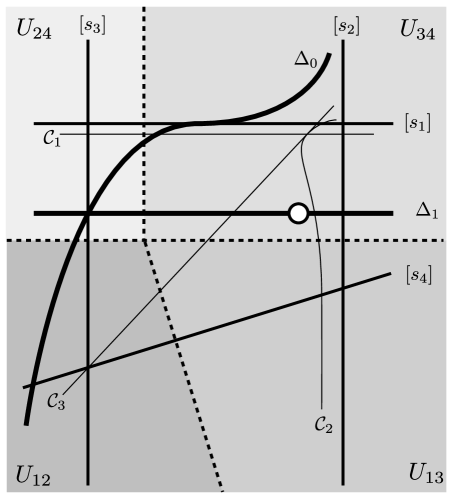
Figure 1: Schematic depiction of the moduli space of the 2-parameter model. Shown are the divisors $[s_{i}]$ and $\Delta_{0,1}$, and their mutual intersections, the coordinate patches $U_{ij}$ and the 2-surfaces $\CC_{i}$ along which our monodromy calculations are done.

To this end, we can choose

$$\begin{split}\CC_{1}&=\{s_{1}-\epsilon_{1}s_{4}^{3}=0\}\\ \CC_{2}&=\{s_{2}-\epsilon_{3}\overline{s_{4}}s_{3}=0\}\\ \CC_{3}&=\{s_{2}s_{4}-\epsilon_{2}s_{3}=0\}\end{split}$$ (5.19)

The $\CC_{i}$ are chosen to meet at our basepoint near the large radius limit, located at $(q_{1},q_{2})=(\epsilon_{1},\epsilon_{2})$, where

$$q_{1}=\frac{s_{1}}{s_{4}^{3}},\qquad q_{2}=\frac{s_{2}s_{4}}{s_{3}}$$

are the good local coordinates in the patch $U_{34}$. Note that $\CC_{2}$ is homotopic to, but is not itself a holomorphic curve in $\CM$. In the local coordinates in $U_{34}$, it is given by

$$C_{2}=\{q_{2}=\epsilon_{3}|s_{4}(q_{1},q_{2})|^{2}\}$$

where $|s_{4}(q_{1},q_{2})|^{2}$ is a complicated function of $q_{1},q_{2}$, given by solving the D-flatness condition (5.16) and

$$\epsilon_{3}=\frac{\epsilon_{2}}{|s_{4}(\epsilon_{1},\epsilon_{2})|^{2}}$$

First consider the 2-surface $\CC_{1}$. It is easy to see that it intersects $\Delta_{0}$ three times, $[s_{2}]$ and $[s_{3}]$ once each, and does not intersect $[s_{1}]$, $[s_{4}]$ or $\Delta_{1}$.

The monodromy around the conifold locus is

$$M_{c}:v\mapsto v-3(v,\CO)\CO$$ (5.20)

As usual, the “3” is because there are three flat line bundles (6-branes) which become massless at the conifold locus. The monodromies about the other two points of intersection with $\Delta_{0}$ are related to this by conjugation with $M_{r_{1}}$,

$$\begin{split}M_{c^{\prime}}:&\ v\mapsto v-3(v,L_{1})L_{1}\\ &=M_{r_{1}}M_{c}M_{r_{1}}^{-1}\\ M_{c^{\prime\prime}}:&\ v\mapsto v-3(v,L_{1}^{2})L_{1}^{2}\\ &=M_{r_{1}}^{2}M_{c}M_{r_{1}}^{-2}\\ \end{split}$$ (5.21)

The monodromy about $[s_{3}]$, therefore is

$$M_{[s_{3}]}=M_{r_{2}}M_{c}M_{c^{\prime}}M_{c^{\prime\prime}}$$ (5.22)

and satisfies

$$M_{[s_{3}]}^{3}=1$$ (5.23)

Similarly, consider $\CC_{2}$. This intersects $[s_{1}]$, $\Delta_{1}$ and $[s_{4}]$. The monodromy about $\Delta_{1}$ is

$$M_{\Delta_{1}}:v\mapsto v-(v,x)x$$ (5.24)

where $x=\CO_{D_{2}}-3\CO_{D_{1}}-3\CO_{E}$. So the monodromy about $[s_{4}]$ is

$$M_{[s_{4}]}=M_{r_{1}}M_{\Delta_{1}}$$ (5.25)

and satisfies

$$M_{[s_{4}]}^{3}=M_{r_{2}}$$ (5.26)

Finally, we turn to $\CC_{3}$. Unlike the previous cases, $\CC_{3}$, or any 2-surface homotopic to it, necessarily crosses $[s_{3}]$ at the LG point (the intersection of $[s_{3}]$ and $[s_{4}]$). Thus it makes sense to talk about the monodromy “about the LG point”. $\CC_{3}$ also intersects $[s_{1}]$, $\Delta_{0}$ and $\Delta_{1}$ each once. So we find the monodromy about the $LG$ point is

$$M_{LG}=M_{r_{1}}M_{c}M_{\Delta_{1}}$$ (5.27)

which satisfies

$$M_{LG}^{9}=1$$ (5.28)

The quantum symmetry at the LG point is enhanced from $\BZ_{3}$ to $\BZ_{3}\times\BZ_{9}$. The $\BZ_{3}$ generator is, of course, tensoring with the flat line bundle $\CL$. The $\BZ_{9}$ generator is $M_{LG}$. The ($L=0$) $B$-type fractional branes at the LG point are the orbit under $\BZ_{3}\times\BZ_{9}$ of the D6-brane, $\CO$. They fall into the K-theory classes,

$$\begin{split}V_{k,m}&=V_{k,3}-m\alpha\\ V_{k,3}&=M_{LG}^{-k}\ V_{9,3}\\ V_{9,3}&=\CO\end{split}$$ (5.29)

or, explicitly,

$$\begin{split}V_{1,3}&=-2\CO-\CO_{D_{1}}+\CO_{E}\\ V_{2,3}&=\CO+\CO_{D_{1}}=L_{1}\\ V_{3,3}&=\CO+3\CO_{D_{1}}-\CO_{D_{2}}+3\CO_{E}\\ V_{4,3}&=-2\CO-7\CO_{D_{1}}+2\CO_{D_{2}}+\CO_{C}-5\CO_{E}\\ V_{5,3}&=\CO+4\CO_{D_{1}}-\CO_{D_{2}}-\CO_{C}+3\CO_{E}-\CO_{p}\\ V_{6,3}&=-2\CO-3\CO_{D_{1}}+\CO_{D_{2}}-3\CO_{E}\\ V_{7,3}&=4\CO+8\CO_{D_{1}}-2\CO_{D_{2}}-\CO_{C}+4\CO_{E}\\ V_{8,3}&=-2\CO-5\CO_{D_{1}}+\CO_{D_{2}}+\CO_{C}-3\CO_{E}+\CO_{p}\\ V_{9,3}&=\CO\end{split}$$

The intersection form

$$(V_{k,m},V_{k^{\prime},m^{\prime}})=f_{k-l}$$ (5.30)

where $f_{n}$ takes values

$n$	$1$	$2$	$3$	$4$	$5$	$6$	$7$	$8$	$9$
$f_{n}$	$-1$	$1$	$-1$	$2$	$-2$	$1$	$-1$	$1$	$0$

The other limit points of the model are as follows. There is the aforementioned large radius point (at the intersection of $[s_{1}]$ and $[s_{2}]$). There’s a hybrid point, consisting of a LG model (with a cubic superpotential) fibered over a $\BP^{2}$, at the intersection of $[s_{1}]$ and $[s_{3}]$. Circling this point about the $[s_{3}]$, we detected in (5.23) the enhanced $\BZ_{3}$ quantum symmetry of the LG fiber; circling this point about $[s_{1}]$, we detect the monodromy, $M_{r_{1}}$, associated to shifting the B-field on the $\BP^{2}$ base. Finally, at the intersection of $[s_{2}]$ and $[s_{4}]$, the Calabi-Yau develops a $\BZ_{3}$ orbifold singularity. The Calabi-Yau isn’t globally a quotient by this $\BZ_{3}$, so we don’t really have an enhanced $\BZ_{3}$ quantum symmetry. Rather, circling $[s_{4}]$ three times is equivalent to shifting the B-field (5.26).

5.4 Branes in the small volume phase

According to the above discussion, D-branes in the small volume phase can be investigated by studying D-branes on the orbifold $\BC^{5}/\BZ_{9}\times\BZ_{3}$. Those can be studied in terms of quiver gauge theory. A basic set of D-branes (with Dirichlet conditions in all directions of the orbifold) is given by the fractional branes, which are labeled by irreducible representations of the orbifold theory. Those form the nodes of the quiver. The chiral matter multiplets, which can be determined in the usual way by projection, give rise to the links of the quiver. Their number can be computed from the index theorem and is equal to the intersection number. This should therefore be compared to the result of a geometric index computation. The continuation of the fractional brane basis to large volume sheaves has been discussed in the literature [23, 28, 29, 30]. In this paper, our focus is on the K theory classes and we’d like to compare the fractional branes to large volume branes whose K-theory classes are $V_{k,m}$.

Let us make this more concrete for the model at hand. Since the $\BZ_{9}\times\BZ_{3}$ orbifold group is abelian, all irreducible representations are one-dimensional and can be labeled by two phases: $\rho=(\exp 2\pi ik/9,\exp 2\pi m/3)$. Working out the representation theory yields the following result: The number of chiral multiplets between a brane $(k,m)$ and a brane $(k^{\prime},m^{\prime})$ depends only on the difference $\Delta k=k-k^{\prime}$. In particular, it is independent of the $m$ label. The dependence on $\Delta k$ is summarized in the following table:

$\Delta k$	1	2	3	4	5	6	7	8	9
	-1	1	-1	2	-2	1	-1	1	0

Comparison with the table in the previous section shows that this exactly reproduces the geometrical intersection numbers of the K-theory classes $V_{k,m}$.

The index computations performed above can be taken to the IR fixed point of the model, which is described by the Gepner model. Let us make the connection to boundary CFT results more explicit.

According to [23], the fractional branes of the quiver discussion should be directly compared to the set of $L=0$ rational Gepner boundary states. For the covering theory, the Gepner model $(k=7)^{3}(k=1)^{2}$, these B-type boundary states have been computed in [17]. The Gepner model itself is a $\BZ_{9}$ orbifold of a tensor product of minimal models (+ other projections, which are currently not of importance to us), the $\BZ_{9}$ being the GSO projection. Accordingly, there is a $\BZ_{9}$ quantum symmetry, which we denote $g$. The boundary states are labeled by a single label $M$, $M=0,2,4,\dots 18$, which can be interpreted as discrete $\BZ_{9}$ Wilson lines. This label should be directly compared to the representation label $k$ in the quiver discussion, $M=2k$. The quantum symmetry acts on the boundary states by $g:M\mapsto M+2$. In geometrical terms this action maps to the action of the Gepner monodromy on six-branes $\CO$.

To determine the intersection matrix, the Witten index ${\rm tr}_{R}(-1)^{F}$ has to be evaluated in the open string Ramond sector. This is related by a modular transformation to the closed string amplitude $<M_{1}|(-1)^{F_{L}}|M_{2}>_{RR}$ between boundary states. To compute the intersection matrix on the covering theory, the formulas given in [16] can be used. Due to the symmetry of the model, it can be written in terms of the shift matrix $g$:

$$I=-3g^{-1}+3g^{-2}-3g^{-3}+6g^{-4}-6g^{-5}+3g^{-6}-3g^{-7}+3g^{-8}$$ (5.35)

From this, the intersection matrix of the orbifold model can be obtained directly. The boundary states of the covering theory are invariant under the $\BZ_{3}$ orbifold action. To obtain consistent boundary states of the orbifold theory, one adds a twisted sector contribution to the boundary states. This part of the boundary state contains only Ishibashi states built on fields in the twisted sector. In the open string sector they lead to projection operators, since the modular transformation of a twisted sector character leads to an insertion of a group element. The boundary states are distinguished by $\BZ_{3}$ representations, which determine how the projections act in the open string sector.

The index in the orbifold model can be determined without explicit knowledge of that boundary state. It is sufficient to know that the orbifold acts freely, which means that there are no RR ground states in the twisted sector. Therefore, the twisted part of the boundary state cannot give rise to new contributions to the index. All that happens is that there is a projection in the open string sector, picking out an invariant combination of the R-ground states counted in (5.35). To write the new intersection matrix, we introduce the operation $h$, which is the quantum symmetry corresponding to the $\BZ_{3}$. In terms of the two quantum symmetry operators the intersection matrix reads:

$$I=\left(g^{-1}+g^{-2}-g^{-3}+2g^{-4}-2g^{-5}+g^{-6}+g^{-7}+g^{-8}\right)(1+h+h^{2}).$$ (5.36)

This matrix is just a different form of presenting the contents of the table in the quiver-based discussion.

The form of the intersection matrix shows that transforming a fractional brane by $h$ cannot change the $\BZ$-valued RR charge, but only the torsion charge.

We are now ready to apply our general considerations of section 3 to construct a torsion brane as a bound state of BPS states.

There are two ways to do so: One way is to take a fractional brane and its $h$-transformed anti-brane. The general discussion of section 3 applies to this example, and this system is tachyon-free. It therefore presents a classically stable state carrying only torsion charge.

Another way is to take a superposition of fractional branes in the following way:

$$|T>=h|B>+\sum_{n=1}^{8}g^{n}|B>,$$ (5.37)

where $|B>$ is any of the fractional branes. There are tachyons propagating between the individual branes, making this configuration unstable. Mapping the brane charges to large volume shows explicitly that there is a net torsion charge and the decay product is therefore non-trivial.

6 The Self-Mirror Example

So far, all of our examples have had $H^{4}(X)_{tor}=0$. This had several simplifying consequences. First, we had that the torsion subgroup $K^{0}(X)_{tor}=H^{2}(X)_{tor}$. That is, torsion elements of the K-theory were just labeled by their (torsion) first Chern classes. Second, the quantum symmetry group acted trivially on $K^{0}(X)_{tor}$, because tensoring with a (flat) line bundle does not change the first Chern class of an object of rank zero.

Table 3: Action of $\BZ_{2}$ on the homology of $K3\times T^{2}$.

Further, because $H^{3}(X)_{tor}$ also vanished (by Poincaré duality), there was no possibility for adding topologically nontrivial discrete torsion. Even in cases (such as the second example of [2]) where the orbifold conformal field theory admitted discrete torsion, the resulting CFT was continuously connected to the CFT without discrete torsion. They lay in the same connected component of the moduli space.

Finally, we had the property that the monodromies in the Kähler moduli space acted trivially on $K^{1}(X)$ (which is why, heretofore, we have mostly talked about $K^{0}(X)$), while the monodromies in the complex structure moduli space acted trivially on $K^{0}(X)$.

To see some of the possibilities when $H^{4}(X)_{tor}\neq 0$, we turn to the Calabi-Yau example of [1]. Here $X=(K3\times T^{2})/\BZ_{2}$ where the $\BZ_{2}$ acts as $(-1)$ on the $T^{2}$ and as a freely-acting holomorphic involution of the $K3$ (under which the holomorphic 2-form is necessarily odd).

Without the $T^{2}$, the quotient $K3/\BZ_{2}$ would be an Enriques surface; with the $T^{2}$, we obtain a Calabi-Yau which has the structure of a $T^{2}$ bundle over the Enriques surface. The holonomy group is $SU(2)\times Z_{2}$ which, being smaller than $SU(3)$, means that the fundamental group is not finite. Rather, $\pi_{1}(X)=\BZ_{2}\semidir(\BZ\times\BZ)$, where $\BZ_{2}:(n,m)\in\BZ\times\BZ\to(-n,-m)$.

The commutator subgroup $[\pi_{1}(X),\pi_{1}(X)]=\BZ^{2}$ of elements of the form $(0,(2m,2n))$. The quotient

$$\homo{1}{X}=\pi_{1}(X)/[\pi_{1}(X),\pi_{1}(X)]=\BZ_{2}^{3}$$ (6.1)

The involution acts on the homology of $K3\times T^{2}$ as in Table 3, where $1$ is the trivial representation, $\sigma$ is the sign representation and $R$ is the regular representation (which, over the integers, is irreducible).

6.1 Computation of the K-theory

Since the cohomology of $X$ was computed in [31], we will just hit the high points of the computation. The $E^{2}$ term of the CLSS is

$$E^{2}_{p,q}=\homo{p}{\BR P^{\infty},\CH_{q}(K3\times T^{2})}$$

where the trivial representation, $1$, leads to the ordinary homology of $\BR P^{\infty}$,

$$\homo{n}{\BR P^{\infty},\BZ}=\begin{cases}\BZ&n=0\\ \BZ_{2}&n=2k+1,\quad k\geq 0\\ 0&\text{otherwise}\end{cases}$$

The sign representation, $\sigma$, leads to the homology with twisted coefficients,

$$\homo{n}{\BR P^{\infty},\widetilde{\BZ}}=\begin{cases}\BZ_{2}&n=2k\\ 0&\text{otherwise}\end{cases}$$

and the regular representation to

$$\homo{n}{\BR P^{\infty},\sheaf{R}}=\begin{cases}\BZ&n=0\\ 0&\text{otherwise}\end{cases}$$

Putting these together with Table 3, yields the $E^{2}$ term,

$$E^{2}_{p,q} \BZ \BZ_{2} 0 \BZ_{2} 0 \BZ_{2}^{2} 0 \BZ_{2}^{2} 0 \BZ_{2}^{2} \BZ^{11}\oplus\BZ_{2}^{2} \BZ_{2} \BZ_{2}^{2} \BZ_{2} \BZ_{2}^{2} \BZ^{24} \BZ_{2}^{4} 0 \BZ_{2}^{4} 0 \dots \BZ^{11}\oplus\BZ_{2}^{2} \BZ_{2} \BZ_{2}^{2} \BZ_{2} \BZ_{2}^{2} \BZ_{2}^{2} 0 \BZ_{2}^{2} 0 \BZ_{2}^{2} \BZ \BZ_{2} 0 \BZ_{2} 0 \dots$$

6

5

4

3

2

1

0

0 1 2 3 4

(6.2)

The differential $d_{2}$ vanishes, but $d_{3}$ is nontrivial. The spectral sequence converges at the $E^{4}$ term, which looks like,

$$E^{4}_{p,q} \BZ 0 0 0 0 0 0 0 0 0 \BZ^{11}\oplus\BZ_{2} \BZ_{2} \BZ_{2} 0 0 \BZ^{24} \BZ_{2}^{2} 0 0 0 \dots \BZ^{11}\oplus\BZ_{2} \BZ_{2} \BZ_{2} 0 0 \BZ_{2}^{2} 0 \BZ_{2}^{2} 0 0 \BZ \BZ_{2} 0 0 0 \dots$$

6

5

4

3

2

1

0

0 1 2 3 4

(6.3)

So we find a filtration of $\homo{1}{X}$ which gives

$$0\to\BZ_{2}^{2}\to\homo{1}{X}\to\BZ_{2}\to 0$$

We have already computed in (6.1) that the extension must be trivial. We also find directly that

$$\homo{2}{X}_{tor}=\BZ_{2}$$

So we have

$$\begin{aligned} \coho{2}{X}&=\BZ^{11}\oplus\BZ_{2}^{3}\\ \coho{4}{X}&=\BZ^{11}\oplus\BZ_{2}\end{aligned}\qquad\begin{aligned} \coho{3}{X}&=\BZ^{24}\oplus\BZ_{2}\\ \coho{5}{X}&=\BZ_{2}^{3}\end{aligned}$$

We can choose a basis for $\coho{2}{X}$ as follows. Let the index $I$ run over ten values, $I=+,-,i=1,\dots,8$. We have generators, $\xi_{0},\xi_{I}$, as well as the torsion generators, $\chi_{0},\chi_{A}$, for $A=1,2$. For $\coho{4}{X}$, we choose: $\eta^{0},\eta^{I}$ and the torsion generator $\phi$. Finally, let $\rho$ be the generator of $\coho{6}{X}$. The ring structure on $\coho{ev}{X}$ is

$$\begin{aligned} \xi_{I}\cup\xi_{J}&=-2C_{IJ}\eta^{0}\\ \xi_{I}\cup\xi_{0}&=-2C_{IJ}\eta^{J}\end{aligned}\qquad\begin{aligned} \xi_{0}\cup\chi_{0}&=\phi\\ \chi_{1}\cup\chi_{2}&=\phi\end{aligned}\qquad\begin{aligned} \xi_{0}\cup\eta^{0}&=\rho\\ \xi_{I}\cup\eta^{J}&=\delta_{I}{}^{J}\rho\end{aligned}$$ (6.4)

where $C_{IJ}$ is a symmetric matrix, whose nonzero entries are $C_{ij}$, the Cartan matrix of $E_{8}$, and $C_{+-}=C_{-+}=-1$.

For $\coho{3}{X}$, we can choose a basis: $\zeta_{AI^{\prime}},\zeta_{Aa}$, for $a=1,2$, and torsion generator $\sigma$. $\coho{5}{X}$ is pure torsion, with generators: $\kappa_{A},\kappa_{0}$.

The ring structure is

$$\begin{aligned} \zeta_{AI^{\prime}}\cup\zeta_{BJ^{\prime}}=-2\epsilon_{AB}C_{I^{\prime}J^{\prime}}\ \rho\\ \zeta_{Aa}\cup\zeta_{Bb}=\epsilon_{AB}(\sigma_{1})_{ab}\ \rho\end{aligned}\qquad\begin{aligned} \xi_{0}\cup\sigma&=\kappa_{0}\\ \chi_{A}\cup\sigma&=\kappa_{A}\end{aligned}$$ (6.13)

where $C_{I^{\prime}J^{\prime}}$ is the same $10\times 10$ matrix as the one which appeared in (6.4) and $\sigma_{1}$ is the Pauli matrix.

Since $\coho{3}{X}_{tor}=\BZ_{2}$, we have the possibility of turning on a topologically-nontrivial flat $B$ field, with $[H]\in\coho{3}{X}_{tor}=\BZ_{2}$. The moduli space has two disconnected components, depending on whether we turn on a nontrivial $[H]$. If we do so, D-brane charge takes values in the twisted K-theory, $K^{\bullet}_{[H]}(X)$. The $E_{2}$ term of the AHSS is exactly the same as in the untwisted case; only the differentials are modified. For our purposes, it suffices to know that

$$d_{3}=Sq^{3}+[H]$$ (6.14)

In our previous paper, we showed rather generally that, for a 6-manifold $X$ with $H^{1}(X)=0$, all of the higher differentials in the AHSS vanish. Since our argument did not invoke the specific form of $d_{3}$ (merely that its image is torsion), it works just as well when $[H]$ is a nonzero torsion element as when it vanishes.

So, in both the twisted and the untwisted cases, we have

$$0\to\coho{5}{X}\to K^{1}(X)\to\coho{3}{X}\to 0$$ (6.15)

for $K^{1}(X)$ and

$$0\to\coho{4}{X}_{tor}\to K^{0}(X)_{tor}\to\coho{2}{X}_{tor}\to 0$$ (6.16)

for the torsion in $K^{0}(X)$. We need to decide whether the extension

$$0\to\BZ_{2}\to K^{0}(X)_{tor}\to\BZ_{2}^{3}\to 0$$

is trivial ($K^{0}(X)_{tor}=\BZ_{2}^{4}$) or nontrivial ($K^{0}(X)=\BZ_{2}^{2}\oplus\BZ_{4}$). That is, we want to know if there is an element of order 4 in the torsion subgroup.

In fact, it is easy to see that no elements of $K^{0}(X)_{tor}$ are order 4. We can explicitly construct the generators

$$\begin{split}\alpha_{A}&=\CL_{A}-\CO\\ \alpha_{0}&=\CL_{0}-\CO\end{split}$$ (6.17)

where $\CL_{A}$ and $\CL_{0}$ are the flat line bundles with first Chern class $\chi_{A}$ and $\chi_{0}$, respectively. The remaining generator is

$$\tilde{\alpha}=\CL_{0}\otimes L+\CO-\CL_{0}-L=a_{0}\otimes\alpha_{0}$$ (6.18)

where $L$ is the line bundle with $c_{1}(L)=\xi_{0}$ and $a_{0}=L-\CO$. This generator has $c_{1}(\tilde{\alpha})=0$, $c_{2}(\tilde{\alpha})=\phi$. Since $\phi$ is not the square of some class in $\coho{2}{X}_{tor}$, $\tilde{\alpha}$ cannot be written as twice some linear combination of the other generators, which is what we would have if (6.16) were a nontrivial extension.

6.2 The moduli space

The vector multiplet and hypermultiplet moduli space is

$$\begin{split}\CM_{V}&=\Gamma_{V}\!\!\left\backslash\frac{O(10,2)}{O(10)\times(2)}\right.\times\frac{SL(2)}{U(1)}\\ \CM_{H}&=\Gamma_{H}\!\!\left\backslash\frac{O(12,4)}{O(12)\times O(4)}\right.\end{split}$$

The modular group $\Gamma_{V}\times\Gamma_{H}$ is roughly the subgroup of the modular group of $K3\times T^{2}$ compactifications which survives the orbifold projection. We will discuss the more precise definition in the following; it will depend on whether certain RR fluxes are turned on.

The symplectic form on $K^{1}(X)/K^{1}(X)_{tor}$ coincides with the standard intersection form on $\coho{3}{X}/$torsion. That is,

$$\Omega=(-2C\oplus\sigma_{1})\otimes(i\sigma_{2})$$ (6.19)

where $C_{I^{\prime}J^{\prime}}$ is the matrix in(6.13) and the $\sigma_{i}$ are the Pauli matrices.

A similar result holds for the intersection form on $K^{0}(X)$, which can be best understood as follows. Let $\pi:X\to\sheaf{E}$ be the projection from $X$ to the Enriques surface, $\sheaf{E}$. Any element $v\in K^{0}(X)$ can be uniquely decomposed as

$$v=\pi^{!}u+(L-\CO)\otimes\pi^{!}\tilde{u}+c^{A}\alpha_{A}$$ (6.20)

where, as above, $L$ is the line bundle with $c_{1}(L)=\xi_{0}$, $u,\tilde{u}\in K^{0}(\sheaf{E})$ and the $c^{A}=0$ or $1$. Representing $v$ by the quadruple $(u,\tilde{u},c^{1},c^{2})$ and $w$ by the quadruple $(x,\tilde{x},d^{1},d^{2})$, a simple computation yields

$$(v,w)=Q(\tilde{u},x)-Q(u,\tilde{x})$$ (6.21)

where $Q(x,y)$ is the symmetric quadratic form on $K^{0}(\sheaf{E})$ given by taking the Dolbeault index on $\sheaf{E}$,

$$Q(x,y)=Ind_{\sheaf}{E}\overline{\partial}_{x\otimes\overline{y}}$$ (6.22)

For later use, it will be helpful to tabulate this quadratic form in some explicit basis for $K^{0}(\sheaf{E})$ (modulo torsion). Choose $\CO,x_{I}=L_{I}-\CO$ and $\CO_{p}$ as a basis. Then

$$\begin{aligned} Q(\CO,\CO)&=1\\ Q(\CO,x_{I})&=-C_{II}\\ Q(\CO,\CO_{p})&=1\end{aligned}\qquad\begin{aligned} Q(x_{I},x_{J})&=2C_{IJ}\\ Q(x_{I},\CO_{p})&=0\\ Q(\CO_{p},\CO_{p})&=0\end{aligned}$$ (6.23)

As we said, $X$ is a $T^{2}$-bundle over an Enriques surface, $\sheaf{E}$. $T^{2}$ has a T-duality group $SL(2,\BZ)\times SL(2,\BZ)$. Doing fiber-wise T-duality is a symmetry of the theory. One of these $SL(2,\BZ)$’s becomes a subgroup of $\Gamma_{V}$; the other is a subgroup of $\Gamma_{H}$. Which is which depends on whether we are studying Type IIA or Type IIB on $X$.

The modular group $\Gamma_{V}=O(10,2,\BZ)\times SL(2,\BZ)$. In the Type IIB description, where the vector multiplet moduli space is the space of complex structures, the $SL(2,\BZ)\subset\Gamma_{V}$ is the “geometrical” one, acting on $\coho{1}{T^{2}}$, i.e. the one which acts on the ‘$A$’ index. In the Type IIA description, the $SL(2,\BZ)\subset\Gamma_{V}$ is the one which permutes $\coho{0}{T^{2}}$ and $\coho{2}{T^{2}}$.

Modulo the (torsion) subgroup of $K^{0}(X)$ generated by the $\alpha_{A}$ (and the corresponding subgroup of $K^{1}(X)$ generated by $\beta_{A}$, the images of the $\kappa_{A}$ in (6.15)), this $SL(2,\BZ)$ is generated by

$$\begin{split}T&:v\mapsto v\otimes L\\ S&:v\mapsto v\otimes(L-\CO)-\pi^{!}\pi_{!}v\end{split}$$ (6.24)

The expression for $S$ is not quite correct as an action on all of $K^{\bullet}(X)$, since it annihilates the $\alpha_{A}$ and the $\beta_{A}$. More correctly, $S$ acts on $K^{0}(X)$ as

$$S:(u,\tilde{u},c^{1},c^{2})\mapsto(-\tilde{u},u,c^{1},c^{2})$$ (6.25a)

and on $$K^{1}(X)$$ as

$$S:\beta_{0}\leftrightarrow\tilde{\beta}$$ (6.25b)

leaving the other generators fixed. Here $$\beta_{0} \kappa_{0} \tilde{\beta} K^{1}(\sheaf{E}) T$$ is the image of in (6.15) and is the pullback of the torsion class in . In the same notation, the action of is

$$\begin{split}T:\ (u,\tilde{u},c^{1},c^{2})&\mapsto(u,\tilde{u}+u,c^{1},c^{2})\\ \tilde{\beta}&\mapsto\tilde{\beta}+\beta_{0}\end{split}$$ (6.25c)

leaving the rest of $K^{1}(X)$ fixed.

It is easy to see that $S,T$ satisfy the desired relations

$$\begin{split}S^{2}&=-1\\ (ST)^{3}&=1\end{split}$$ (6.26)

and preserve both the intersection pairing and the torsion pairing.

More subtly, they also commute with the $\BZ_{2}$ quantum symmetry (when one views the theory on $X$ as a $\BZ_{2}$ orbifold of the theory on $K3\times T^{2}$). The action of the quantum symmetry is generated by

$$v\mapsto v\otimes\CL_{0}$$ (6.27)

Clearly, this commutes with the action of $T$. In the above decomposition, it acts as

$$(\BZ_{2})_{Q}:(u,\tilde{u},c^{1},c^{2})\mapsto(u\otimes\CL,\tilde{u}\otimes\CL,c^{1},c^{2})$$ (6.28)

where $\CL$ is the flat nontrivial line bundle on the Enriques surface, and it acts trivially on $K^{1}(X)$. Thus it also commutes with the action of $S$.

Note that the first $SL(2,\BZ)$ acts trivially on $K^{0}(X)/K^{0}(X)_{tor}$ and the second acts trivially on $K^{1}(X)/K^{1}(X)_{tor}$ But both act nontrivially on the torsion subgroups. The torsion elements, $\alpha_{A}=\CL_{A}-\CO\in K^{0}(X)_{tor}$ and $\beta_{A}\in K^{1}(X)_{tor}$, transform as doublets under the first $SL(2,\BZ)$.

Under the second $SL(2,\BZ)$, the torsion classes $\alpha_{0}$ and $\tilde{\alpha}$ transform as a doublet as do torsion branes, $\beta_{0},\tilde{\beta}\in K^{1}(X)_{tor}$.

Note that this is exactly the situation anticipated in [2]. It is simply not true that $K^{0}$ is held fixed when we move about in the complex structure moduli space, and $K^{1}$ is held fixed as we move about in the Kähler moduli space. Rather, both undergo monodromies. Only after modding out by the torsion do we find that $K^{0}/K^{0}_{tor}$ is held fixed when we move about in the complex structure moduli space, and $K^{1}/K^{1}_{tor}$ is held fixed as we move about in the Kähler moduli space.

6.3 Fluxes

In [1], the authors argue that, to obtain a simple heterotic dual, one needs to turn on certain RR fluxes. In the Type IIA description (so that the fluxes are elements of $K^{0}(X)$), we can turn on a flux in class $\alpha_{0}$. That is, we consider turning on a $\BZ_{2}$ Wilson line for the RR gauge field.

Under the action of the modular group, $\alpha_{0}$ is not invariant. Its orbit under the $SL(2,\BZ)\subset\Gamma_{V}$ consists of three elements, $\alpha_{0},\tilde{\alpha}$ and $\alpha_{0}+\tilde{\alpha}$. Before modding out by $\Gamma_{V}$, the moduli space consists of four disconnected components, one with no RR flux turned on, and three more with the above RR fluxes turned on. The subgroup $\Gamma(2)\subset SL(2,\BZ)$ preserves these RR fluxes and the quotient group $SL(2,\BZ)/\Gamma(2)$ identifies the different components. The upshot is that the moduli space with RR flux turned on, rather than having three disconnected components, has a single connected component

$$\CM_{V}^{RR}=\tilde{\Gamma}_{V}\!\!\left\backslash\frac{O(10,2)}{O(10)\times O(2)}\right.\times\frac{SL(2)}{U(1)}$$ (6.29)

where

$$\tilde{\Gamma}_{V}=O(10,2,\BZ)\times\Gamma(2)$$ (6.30)

In particular, $\CM_{V}^{RR}$ is a finite cover of the previously-discussed vector multiplet moduli space with no RR flux turned on.

In [3], it was argued that turning on a discrete RR flux $f\in K^{\bullet}(X)_{tor}$ restricts the allowed D-brane charges in the theory. It is a little hard to directly compare their results to ours, as they are interested in the equivariant K-theory of orbifolds which cannot be resolved to smooth manifolds. The condition they proposed was that only those charges, $v$, which satisfy

$$f\otimes v=0$$ (6.31)

are allowed. The set of such $v$’s forms a subgroup of $K^{\bullet}(X)$. As we will see in the next section, this proposal does not seem to give the right answer in the case we are interested in. Instead, we propose that the correct group of D-brane charges is

$$K^{\bullet}(X)/\Gamma_{f}$$ (6.32a)

where $$\Gamma_{f} K^{\bullet}(X)$$ is the (torsion) subgroup of given by

$$\Gamma_{f}=\{v\in K^{\bullet}(X)\ \text{such that}\ v=f\otimes w\ \text{for some}\ w\}$$ (6.32b)

In the present instance, $f=\alpha_{0}$, and the restriction (6.31) is that the coefficient of $a_{0}=L-\CO$ in the charge must be even. There is no restriction on the charges in $K^{1}(X)$. In terms of the decomposition $v=(u,\tilde{u},c^{1},c^{2})$ of (6.20), it means that the element $\tilde{u}\in K^{0}(\sheaf{E})$ has even rank. And, indeed, the $\Gamma(2)$ subgroup of $SL(2,\BZ)$ preserves this condition on $\tilde{u}$.

The restriction (6.32) in our case is less drastic. The image of $f\otimes$ is

$$\Gamma_{f}=\{0,\tilde{\alpha}\}$$ (6.33)

and our proposal for the group of D-brane charges is the quotient of the K-theory by this $\BZ_{2}$ subgroup.

In terms of the decomposition $v=(u,\tilde{u},c^{1},c^{2})$, this quotient is simply expressed by saying that $\tilde{u}\in K^{0}(\sheaf{E})/K^{0}(\sheaf{E})_{tor}$. The quantum symmetry (6.28) should, then, be thought of as acting by

$$(\BZ_{2})_{Q}:(u,\tilde{u},c^{1},c^{2})\mapsto(u\otimes\CL,\tilde{u},c^{1},c^{2})$$ (6.34)

The quantum symmetry in this Type IIA description seems to be related in a simple, but nontrivial way to the quantum symmetry of the heterotic dual theory,

$$(\BZ_{2})_{Q}^{HET}=(\BZ_{2})_{Q}\cdot(-1)^{\text{rank}(\tilde{u})}$$

6.4 Singularities

6.4.1 $\CN=4$ degenerations

Recall that $X$ is a $T^{2}$ fiber bundle over the Enriques surface, $\sheaf{E}$. Say, in Type IIA, we tune the Kähler moduli so that a genus-zero curve in the base, $C\subset\sheaf{E}$, shrinks to zero size. The local geometry of $X$ at such a singularity is just $T^{2}\times(\BC^{2}/\BZ_{2})$. This local geometry preserves $d=4$, $\CN=4$ supersymmetry. D2-branes wrapping the curve $C$ become massless in this limit and give rise to an $\CN=4$ $SU(2)$ gauge theory [1]. That is, quantizing these D2-branes yields (in $\CN=2$ language) massless vector multiplets and a massless hypermultiplet in the adjoint.

The monodromy about this locus is easy to compute. From (6.23), we have $Q(\CO_{C},\CO_{C})=4$ and $Q(u,\CO_{C})\in 2\BZ$ for any $u\in K^{0}(\sheaf{E})$. The monodromy is

$$M_{C}:(u,\tilde{u},c^{1},c^{2})\mapsto(u-\tfrac{1}{2}Q(u,\CO_{C})\CO_{C},\tilde{u}-\tfrac{1}{2}Q(\tilde{u},\CO_{C})\CO_{C},c^{1},c^{2})$$ (6.35)

By the above remark, $\tfrac{1}{2}Q(x,\CO_{C})$ is always an integer, so the above formula makes sense. As expected, since the singular locus in question is a $\BZ_{2}$ orbifold locus in the moduli space, $M_{C}$ satisfies

$$M_{C}^{2}=1$$ (6.36)

If you wish, you can cast (6.35) in the form of (2.13), for $n=0$, by taking

$$\begin{split}y&=(0,\CO_{C},0,0)\\ x\ ``&{=}"\ \tfrac{1}{2}(\CO_{C},0,0,0)\end{split}$$

If we were considering $K3\times T^{2}$, instead of its quotient, $X$, we would have $Q(\CO_{C},\CO_{C})=2$ and we could write down an honest formula of the form (2.13), with no pesky factors of $\tfrac{1}{2}$.

The attentive reader will note that the monodromy (6.35) does not commute with the $SL(2,\BZ)$ action (6.25) (or even with its $\Gamma(2)$ subgroup). This should be obvious from the physical description that we have given of the singularity. The $SL(2,\BZ)$ of (6.25) mixes D2-branes wrapped on $C$ with D4-branes wrapped on $T^{2}\times C$. (6.35) describes the monodromy along a path circling the complex codimension-one locus where the D2-brane wrapped on $C$ becomes massless. Conjugating $M_{C}$ with $S$ in (6.35a), we obtain the monodromy along a different path through the moduli space: the one such that, at the singularity, D4-branes wrapped on $T^{2}\times C$ become massless.

At higher codimension in the moduli space, we obtain $\CN=4$ ADE singularities, of a form that should now be quite familiar.

6.4.2 $\CN=2$ degenerations

As studied in [1, 31, 33], there is another class of singularity in the moduli space, associated to the entire Enriques surface $\sheaf{E}$ collapsing to zero size. Because the singularity is no longer localized on $\sheaf{E}$, the physics of the singularity is sensitive to the fact that the $T^{2}$ bundle over $\sheaf{E}$ is twisted. So, instead of obtaining an $\CN=4$ supersymmetric spectrum of massless states (a vector multiplet and an adjoint hypermultiplet), the twisting breaks $\CN=4$ to $\CN=2$ and the massless states are an $SU(2)$ vector multiplet with $N_{f}=4$ hypermultiplets in the fundamental representation [1].

How does this come about? To understand it, we need to make a little digression about divisors on $X$, in particular those which, under the projection $\pi:X\to\sheaf{E}$, cover the Enriques.

A section of this fiber bundle would give an embedding of Enriques in $X$, whose image would be a divisor in $X$ which projects down to a single copy of $\sheaf{E}$. Since the fiber bundle is nontrivial, there “generically” won’t be a section. However, the transition functions of the fiber bundle act as $-1$ on the $T^{2}$ fibers. This has 4 fixed points on $T^{2}$ and, if we choose the local section to land at one of these fixed points, the result pieces together to a global section $i:\sheaf{E}\hookrightarrow X$. This gives us four divisors, $D_{i,j}$, $i,j=0,1$, in $X$ labeled by the fixed points of the $\BZ_{2}$ action on $T^{2}$. If we wrap a D4-brane on one of these divisors, we have a BPS brane with charge

$$\begin{split}\CO_{D_{0,0}}&=L-\CO\\ \CO_{D_{1,0}}&=L-\CO+\alpha_{1}\\ \CO_{D_{0,1}}&=L-\CO+\alpha_{2}\\ \CO_{D_{1,1}}&=L-\CO+\alpha_{1}+\alpha_{2}\end{split}$$ (6.37)

where the $\alpha_{A}$ of (6.17) are the torsion elements of $K^{0}(X)$ which transform under the “geometrical” $SL(2,\BZ)$ action on the torus (the $SL(2,\BZ)$ which is part of $\Gamma_{H}$).

These branes had a trivial line bundle on their world-volume. But the Enriques surface also has a flat, but nontrivial, line bundle, $\CL$, and we would just as well have gotten a BPS brane by wrapping a D-brane with $\CL$ on its world-volume. These give four more BPS brane, with charges

$$\begin{split}\CL_{D_{0,0}}&=L-\CO+\tilde{\alpha}\\ \CL_{D_{1,0}}&=L-\CO+\alpha_{1}+\tilde{\alpha}\\ \CL_{D_{0,1}}&=L-\CO+\alpha_{2}+\tilde{\alpha}\\ \CL_{D_{1,1}}&=L-\CO+\alpha_{1}+\alpha_{2}+\tilde{\alpha}\end{split}$$ (6.38)

The quantum symmetry (6.27) acts to exchange the branes (6.37) with the corresponding branes (6.38).

Another possibility for finding a divisor in $X$ which covers $\sheaf{E}$ is to choose a pair of points $(z,-z)$ in the fiber, which are exchanged by the $\BZ_{2}$ transition functions. This pieces together to a divisor, $D_{W}$ in $X$ which double-covers $\sheaf{E}$. The normal bundle to $D_{W}$ in $X$ is trivial (we can vary $z$), so $D_{W}$ has trivial canonical bundle. $D_{W}$ double-covers $\sheaf{E}$, so it is a K3 surface. A D4-brane wrapped on $D_{W}$ has charge

$$\CO_{D_{W}}=2(L-\CO)$$ (6.39)

This is twice the charge of one of the branes in (6.37),(6.38). (Multiplying by 2 wipes out the torsion charge.)

This is almost the spectrum of wrapped D-branes that we want. The branes wrapped on $D_{W}$ give rise to massive vector multiplets which, when the Enriques shrinks to zero size, produce an enhanced $SU(2)$ gauge symmetry. The branes wrapped on the $D_{i,j}$ yield hypermultiplets in the fundamental of $SU(2)$.

Unfortunately, between (6.37) and (6.38), we seem to have produced two times too many of them. But, of course, we have yet to implement the fact that we have turned on a discrete RR flux.

Turning on the RR flux $f=\alpha_{0}$ changes the spectrum of allowed D-branes. In §6.3, we discussed two proposals, (6.31),(6.32), for what this restriction might be. Let us see what each of them imply in the present context.

Imposing the condition (6.31) has no effect on the branes wrapped on $D_{W}$. But it does project out all of the singly-wrapped branes on the $D_{i,j}$. If you took a trivial rank-2 bundle on one of the $D_{i,j}$, this could simply decay into a rank-1 trivial bundle on the double-cover and move off the fixed point to become a rank-1 trivial bundle on $D_{W}$. In other words, that does not correspond to a brane “stuck” to this divisor. Instead, we can take the flat, but nontrivial rank-2 bundle $\CO\oplus\CL$ on $D_{i,j}$. This cannot decay to a rank-1 bundle on $D_{W}$; it is genuinely stuck on the Enriques. Unfortunately, it also has twice the charge of a field in the fundamental (i.e. it has the same charge as the $W$ bosons which come from wrapping a 4-brane on $D_{W}$). That is clearly not what the physics requires.

Instead, let us see what (6.32) implies. Here we find that we must mod out by $\Gamma_{f}=\{0,\tilde{\alpha}\}$. That is, we should identify the branes (6.37) with the corresponding branes (6.38). This also gives us four distinct branes wrapping the different $D_{i,j}$, but this time these branes have the right charges to be in the fundamental representation of $SU(2)$. Note also that the modular group (the subgroup of $SL(2,\BZ)$ which commutes with the flavour symmetry) for $N_{f}=4$ was found by Seiberg and Witten [34] to be $\Gamma(2)$. This, too, is in accord with (6.32), rather than (6.31), which is invariant under the larger group, $\Gamma_{0}(2)$.

While we don’t have a rigorous proof, we believe that the monodromy about this locus takes the form

$$M:(u,\tilde{u},c^{1},c^{2})\mapsto(u-2Q(u,\CO)\CO,\tilde{u}-2Q(\tilde{u},\CO)\CO,c^{1},c^{2})$$ (6.40)

This preserves the relevant pairings and gives the right monodromy in the field theory limit [34].

References

- [1] S. Ferrara, J. Harvey, A. Strominger, and C. Vafa, “Second quantized mirror symmetry,” Phys. Lett. B361 (1995) 059, hep-th/9505162.
- [2] J. Distler and I. Brunner, “Torsion D-branes in nongeometrical phases,” hep-th/0102018.
- [3] J. de Boer et al., “Triples, fluxes, and strings,” hep-th/0103170.
- [4] J. Majumder and A. Sen, “Non-BPS D-branes on a Calabi-Yau orbifold,” JHEP 09 (2000) 047, hep-th/0007158.
- [5] M. Mihailescu, K. Oh, and R. Tatar, “Non-BPS branes on a Calabi-Yau threefold and Bose-Fermi degeneracy,” JHEP 02 (2000) 019, hep-th/9910249.
- [6] D.-E. Diaconescu, G. Moore, and E. Witten, “ gauge theory, and a derivation of K-theory from M-theory,” hep-th/0005090.
- [7] O. Bergman, E. Gimon, and S. Sugimoto, “Orientifolds, RR torsion, and K-theory,” JHEP 05 (2001) 047, hep-th/0103183.
- [8] O. Bergman, E. Gimon, and B. Kol, “Strings on orbifold lines,” JHEP 05 (2001) 019, hep-th/0102095.
- [9] M. Atiyah, V. Patodi, and I. Singer, “Spectral asymmetry and Riemannian geometry. I,” Math. Proc. Camb. Phil. Soc. 77 (1975) 43.
- [10] M. Atiyah, V. Patodi, and I. Singer, “Spectral asymmetry and Riemannian geometry. II,” Math. Proc. Camb. Phil. Soc. 78 (1975) 405.
- [11] M. Atiyah, V. Patodi, and I. Singer, “Spectral asymmetry and Riemannian geometry. III,” Math. Proc. Camb. Phil. Soc. 79 (1976) 71.
- [12] J. Lott, “ index theory,” Comm. Anal. Geom. 2 (1994) 279–311.
- [13] C. Vafa, “Quantum symmetries of string vacua,” Mod. Phy. Lett. A4 (1989) 1615.
- [14] S. Katz, D. R. Morrison, and M. R. Plesser, “Enhanced gauge symmetry in type II string theory,” Nucl. Phys. B477 (1996) 105–140, hep-th/9601108.
- [15] A. Klemm and P. Mayr, “Strong coupling singularities and non-abelian gauge symmetries in string theory,” Nucl. Phys. B469 (1996) 37–50, hep-th/9601014.
- [16] I. Brunner, M. R. Douglas, A. Lawrence, and C. Römelsberger, “D-branes on the quintic,” JHEP 08 (2000) 015, hep-th/9906200.
- [17] A. Recknagel and V. Schomerus, “D-branes in Gepner models,” Nucl. Phys. B531 (1998) 185–225, hep-th/9712186.
- [18] M. R. Douglas, B. Fiol, and C. Römelsberger, “Stability and BPS branes,” hep-th/0002037.
- [19] Y. Oz, T. Pantev, and D. Waldram, “Brane-antibrane systems on Calabi-Yau spaces,” hep-th/0009112.
- [20] H. Park. private communication and to appear.
- [21] R. Gopakumar and C. Vafa, “Branes and fundamental groups,” Adv. Theor. Math. Phys. 2 (1998) 399–411, hep-th/9712048.
- [22] M. R. Douglas, B. Fiol, and C. Römelsberger, “The spectrum of BPS branes on a noncompact Calabi-Yau,” hep-th/0003263.
- [23] D.-E. Diaconescu and M. R. Douglas, “D-branes on stringy Calabi-Yau manifolds,” hep-th/0006224.
- [24] A. Beauville, “A Calabi-Yau threefold with non-Abelian fundamental group,” alg-geom/9502003.
- [25] D. R. Morrison, “Geometric aspects of mirror symmetry,” math.ag/0007090.
- [26] M. Kontsevich, “Homological algebra of mirror symmetry,” ICM Zurich (1994) alg-geom/9411018.
- [27] R. P. Horja, “Hypergeometric functions and mirror symmetry in toric varieties,” math.AG/9912109.
- [28] P. Mayr, “Phases of supersymmetric D-branes on Kähler manifolds and the McKay correspondence,” hep-th/0010223.
- [29] S. Govindarajan and T. Jayaraman, “D-branes, exceptional sheaves and quivers on Calabi-Yau manifolds: From Mukai to McKay,” hep-th/0010196.
- [30] A. Tomasiello, “D-branes on Calabi-Yau manifolds and helices,” hep-th/0010217.
- [31] P. Aspinwall, “An dual pair and a phase transition,” Nucl. Phys. B460 (1996) 057, hep-th/9510142.
- [32] J. Distler and J. Gomis. work in progress.
- [33] J. A. Harvey and G. Moore, “Exact gravitational threshold correction in the FHSV model,” Phys. Rev. D57 (1998) 2329–2336, hep-th/9611176.
- [34] N. Seiberg and E. Witten, “Monopoles, duality and chiral symmetry breaking in supersymmetric QCD,” Nucl. Phys. B431 (1994) 484–550, hep-th/9408099.