Abstract

We study domain walls in two different extensions of super Yang–Mills characterized by the absence of a logarithmic term in their effective superpotential. The models, defined by the usual gaugino condensate and an extra field $Y$, give different patterns of domain walls despite both leading to the same effective limit for heavy $Y$, i.e. the Veneziano–Yankielowicz effective Lagrangian of super Yang–Mills. We explain the origin of those differences and also give a physical motivation for introducing the field $Y$.

1 Introduction

The dynamics of strongly coupled theories is a very interesting topic which has been the subject of detailed investigation for many years. It is now believed that the presence of supersymmetry (SUSY) helps in improving our understanding of these theories, by giving us a better insight into issues such as non-perturbative effects and the dynamics of confinement. In that respect SUSY would be not so much a phenomenologically relevant symmetry but a tool through which we could improve our knowledge of the structure of the theory.

In particular supersymmetric Yang–Mills theory (SYM), the theory of gluons and their SUSY partners, the gluinos, offers a very attractive feature, namely the possibility of obtaining exact results despite it being a strongly coupled theory. In 1996 Dvali and Shifman [1] studied the formation of domain walls in this model and estimated the energy of such objects when the walls were BPS-saturated (in which case also one half of the supersymmetry is preserved on the wall). Domain walls arise because SYM has $T({\rm G})$ degenerate vacua, where $T({\rm G})$ is the Dynkin index for the group G in the adjoint representation . At some scale $\Lambda$ the theory enters a strong coupling regime and gaugino condensates form, breaking the $Z_{2N}$ symmetry down to $Z_{2}$. The gaugino condensate has been studied in detail for many years and by several groups using different methods [2]. Given $\lambda_{a}$, the gaugino field, we define the condensate as

$$\langle\lambda\lambda\rangle\equiv\langle{\rm Tr}\lambda^{a}\lambda_{a}\rangle=\Lambda^{3}e^{i\frac{2\pi}{N}k}\;\;\;,k=0,\ldots,N-1\;\;.$$ (1)

However if one wants to study SYM any further, it is necessary to find an effective description in terms of composite superfields. This was done in the early Eighties by Veneziano and Yankielowicz (VY) [3] and the resulting Lagrangian is

$${\cal L}=\frac{1}{4}\int d^{4}\theta{\cal K}+\frac{1}{2}\left[\int d^{2}\theta{\cal W}+{\rm h.c.}\right]\;\;,$$ (2)

where

$${\cal K}=(S\bar{S})^{1/3}\;\;,$$ (3)

is the Kähler potential and

$${\cal W}=\frac{2}{3}S\left(\ln\left(\frac{S}{\Lambda^{3}}\right)^{N}-N\right)\;\;,$$ (4)

is the superpotential, where $S$ is the composite chiral superfield whose lowest component is the gaugino condensate

$$S\equiv\frac{3}{32\pi^{2}}\langle{\rm Tr}(\omega_{\alpha}\omega^{\alpha})\rangle=\frac{3}{32\pi^{2}}\langle{\rm Tr}(\lambda_{\alpha}\lambda^{\alpha})\rangle+\ldots$$ (5)

The structure of ${\cal W}$ is uniquely determined by the anomaly and the symmetries of the theory. Although this Lagrangian is perfectly adequate to reproduce the vacuum structure of SYM, two major problems arise when one tries to use it to study the dynamics of the gaugino condensates. The first one is the lack of $Z_{N}$ invariance of the superpotential (4), which was pointed out by Kovner and Shifman [4] a few years back. The second problem is related to the presence of the logarithm in Eq. (4), which results in the multivaluedness of the scalar potential. This problem was addressed (and solved) in the context of the linear multiplet formulation of gaugino condensation with a field dependent coupling [5]. In the chiral formulation, the concept of the glued potential was proposed in Ref. [4], and further developed in Ref. [6], to cure both problems. However, it was pointed out in this latter reference how the presence of cusps (points where the effective potential is continuous but non-differentiable) between the different vacua of the model would constitute a problem when trying to construct domain walls.

It therefore seems that the VY approach is somehow incomplete and we should be trying to incorporate new degrees of freedom in the effective description of SYM. Several proposals along this line have been put forward in previous years, and a certain degree of success has been achieved in applying them to the construction of domain walls. Promoting the scale parameter $\Lambda$ to a dynamical field (the glueball order parameter) was one of them [7], which resulted in the construction of BPS-saturated domain walls in the large-$N$ limit [8] by exploiting the similarity of these models to a certain kind of Landau–Ginzburg construction. Another option is to incorporate chiral matter fields to the VY Lagrangian, something that was already considered in the Eighties by Taylor, Veneziano and Yankielowicz (TVY) [9]. The idea is to study this model in its Higgs phase (i.e. for small values of the masses of the matter fields) and try to recover the VY limit when this mass parameter gets large. A lot of work has been devoted to following this approach in the context of building domain walls [10, 11, 12, 13, 14]. In particular [11] it is possible to construct BPS-saturated domain walls for any value of the mass parameter (and, therefore, obtain an effective VY limit) only when the number of matter flavours, $N_{f}$, is less than $N/2$ and, moreover, the logarithmic branch of the superpotential is crossed if $N_{f}>1$. Although ways were found of circumventing these obstructions [12, 14], the presence of the logarithm with its different possible branches is still not totally understood, and it would be desirable to find an alternative formulation where no logarithms were present other than in the limit were the VY theory was recovered. This is precisely the goal of this paper. A more ambitious objective would be to identify the extended models and new fields we introduce with already known physical systems. In particular, there has been a lot of work in recent years devoted to the connection between BPS-saturated domain walls and branes, starting with the work of Witten [15], and we shall explore whether any connections are possible between our constructions, done in the low-energy field theory, and other studies performed in the context of string or M-theory [16], and also in the presence of higher supersymmetries [17, 18].

In Section 2 we present two interpolating models, which we denote as Landau–Ginzburg-like, with their different interesting limits, one of which is precisely VY. In Section 3 we start by presenting a simple example, with $N=3$, in order to illustrate the different aspects of the calculation, followed by a detailed discussion of more general results obtained in both models. In Section 4 we motivate them from the physical point of view, and in Section 5 we study the large-$N$ expansion in the VY effective limit. We conclude in Section 6. We have also included a pair of Appendices, one explaining the numerical methods used to construct the domain walls, and the other supplying a detailed analysis of the BPS constraint equations.

2 Interpolating models

In this section we present two model supersymmetric field theories which interpolate between the Veneziano–Yankielowicz (VY) effective Lagrangian for supersymmetric Yang–Mills theory (SYM), and the so-called $A_{N}$ Landau–Ginzburg models.

Let us consider the following superpotential which, from now on, will be referred to as Model I,

$${\cal W}(S,Y)=S\left(\left(\frac{\Lambda^{3}}{S}\right)^{N}e^{-Y/M+N-1}+\frac{Y}{M}\right)\;\;,$$ (6)

with $\Lambda$ and $M$ two mass parameters. We will assume a canonical Kähler potential for the dimension one fields $\phi=S^{1/3}$ and Y, i.e.

$${\cal K}(S,\bar{S},Y,\bar{Y})=(S\bar{S})^{1/3}+Y\bar{Y}\;\;.$$ (7)

Notice that the superpotential transforms as ${\cal W}\rightarrow e^{i\,2\pi/N}\,{\cal W}$ when $S\rightarrow e^{i\,2\pi/N}\,S$, which generates a $Z_{N}$ symmetry in the Lagrangian. The supersymmetric vacua of this theory are given by solutions to the equations ${\mathcal{W}}_{S}=0$ and ${\mathcal{W}}_{Y}=0$, where

$${\mathcal{W}}_{S} = (1-N)\left(\frac{\Lambda^{3}}{S}\right)^{N}e^{-Y/M+N-1}+\frac{Y}{M}\;\;,$$ (8)

$${\mathcal{W}}_{Y} = \frac{S}{M}\left(-\left(\frac{\Lambda^{3}}{S}\right)^{N}e^{-Y/M+N-1}+1\right)\;\;.$$ (9)

There are $N$ such solutions,

$$Y^{a}_{*}=M(N-1),\quad S^{a}_{*}=\Lambda^{3}e^{i2\pi a/N},$$ (10)

with $a=0,1,\dots,N-1$, which spontaneously break the $Z_{N}$ symmetry. In these minima, the superpotential is given by ${\mathcal{W}}_{a}=NS^{a}_{*}$.

The mass eigenstates are most easily found in terms of the $\phi$ and $Y$ fields. The mass matrix ${\mathbf{M}}$ is given by ${\mathbf{M}}={\mathbf{W}}{\mathbf{W}}^{\dagger}$, where ${\mathbf{W}}$ is the matrix of second derivatives of the superpotential

$${\mathbf{W}}=\left(\begin{array}[]{cc}{\mathcal{W}}_{\phi\phi}&{\mathcal{W}}_{\phi Y}\\ {\mathcal{W}}_{Y\phi}&{\mathcal{W}}_{YY}\end{array}\right).$$ (11)

In the vacuum $(S_{*}^{0},Y_{*})$,

$${\mathbf{W}}_{*}^{0}=\left(\begin{array}[]{cc}9N(N-1)\Lambda&3N\Lambda^{2}/M\\ 3N\Lambda^{2}/M&\Lambda^{3}/M^{2}\end{array}\right).$$ (12)

In the limits of small and large $\Lambda/M$, one can straightforwardly show that

$$~{}m^{2}_{Y}\to{\Lambda^{6}}/{M^{4}(N-1)^{2}}, m^{2}_{\phi}\to 81N^{2}(N-1)^{2}\Lambda^{2}\quad(\Lambda\to 0)$$

$$m^{2}_{Y}\to\Lambda^{6}/M^{4},\phantom{N-1)^{2}} m^{2}_{\phi}\to 81N^{2}\Lambda^{2}\phantom{N-1)^{2}}\quad(\Lambda\to\infty)\;\;.$$

Hence

$$\frac{m_{Y}}{m_{\phi}}\sim{\cal O}\left[\frac{\Lambda}{M}\right]^{2}\;\;.$$ (14)

From now on we will work in $M=1$ units. Then, for large values of $\Lambda$, $Y$ is a heavy field. We can therefore integrate it out by imposing ${\mathcal{W}}_{Y}=0$, where ${\mathcal{W}}_{Y}$ is given in Eq. (9). Substituting the resulting solution for $Y$ in terms of $S$ into the superpotential (6) we get the VY superpotential of Eq. (4), up to an unimportant constant factor,

$${\cal W}_{\rm VY}(S)=S\left(\ln\frac{S^{N}}{\Lambda^{3N}}-N\right)\;\;.$$ (15)

On the other hand, if we assume $\Lambda\ll 1$, then $S$ is a heavy field, and we could impose ${\mathcal{W}}_{S}=0$ to obtain

$${\cal W}_{\rm eff}(Y)=N\Lambda^{3}\left(\frac{Y}{N-1}\right)^{1-1/N}e^{-Y/N+1-1/N}\;\;.$$ (16)

The resulting potential has a single minimum at $Y=N-1$, as is expected, which means that the trajectories described by $Y$ start and end up at the same point. Moreover, it can be checked that, in the limit $\Lambda\to 0$, the field barely moves from that point. Therefore it is a good approximation to freeze $Y$ at its vacuum value, to obtain an effective superpotential

$${\mathcal{W}}_{\rm LG1}=S\left(\left(\frac{\Lambda^{3}}{S}\right)^{N}+N-1\right)\;\;.$$ (17)

The effective theory now has a form similar to a $Z_{N}$ symmetric Landau–Ginzburg model (hence the notation), although it is not usual to see negative powers of the field.

Alternatively, one can consider the following superpotential (our, from now on, Model II),

$${\cal W}(S,Y)=S\left(\left(\frac{S}{\Lambda^{3}}\right)^{N}e^{Y/M-N-1}-\frac{Y}{M}\right)\;\;,$$ (18)

which can be obtained from Eq. (6) by just changing ($N\rightarrow-N,\,Y\rightarrow-Y$ ). Hence, there are also $N$ minima

$$Y^{a}_{*}=N+1,\quad S^{a}_{*}=\Lambda^{3}e^{i2\pi a/N}\;\;,$$ (19)

with $a=0,1,\dots,N-1$, which spontaneously break the $Z_{N}$ symmetry. The superpotential in these minima is given by ${\mathcal{W}}_{*}=-NS_{*}$. It is easy to check that the same hierarchy between the $S$ and $Y$ masses appears in the large/small $\Lambda$ limit. On top of that, there is also a $Z_{N}$ conserving minimum given by $(Y_{*}=0,S_{*}=0)$. Whereas for large $\Lambda$ we get the same VY limit of Eq. (15), at small values of $\Lambda$ the model approaches a conventional Landau–Ginzburg model

$${\mathcal{W}}_{\rm LG2}=S\left(\left(\frac{S}{\Lambda^{3}}\right)^{N}-N-1\right).$$ (20)

Hence we have come up with two different two-field models which, in the limit $\Lambda\gg 1$ coincide with the VY Lagrangian, without the ambiguity of a multivalued logarithm and, as far as solutions to the field equations for $S$ go, become Landau–Ginzburg models in the limit $\Lambda\ll 1$.

3 Construction of the domain walls

Let us study the domain wall spectrum of these models. As we are considering static solutions, we wish to minimize the static surface energy functional

$$\sigma=\frac{1}{2}\int dz\left({\mathcal{K}}_{S\bar{S}}\partial_{z}S\partial_{z}\bar{S}+{\mathcal{K}}_{Y\bar{Y}}\partial_{z}Y\partial_{z}\bar{Y}+V(S,Y,\bar{S},\bar{Y})\right)\;\;,$$ (21)

where ${\mathcal{K}}_{J\bar{J}}=\partial^{2}{\mathcal{K}}/\partial J\partial\bar{J}$, $J=S,Y$ is the corresponding Kähler metric. From now on we assume that the wall spreads along the $xy$ plane and, therefore, the profile is calculated along the $z$ direction. The scalar potential $V$ is given by

$$V={\mathcal{K}}^{-1}_{S\bar{S}}|{\mathcal{W}}_{S}|^{2}+{\mathcal{K}}^{-1}_{Y\bar{Y}}|{\mathcal{W}}_{Y}|^{2}\;\;.$$ (22)

As is well known  [19, 20], this can be rewritten as

$$\sigma=\frac{1}{2}\int dz\left({\mathcal{K}}_{S\bar{S}}\left|\partial_{z}\bar{S}-{\mathcal{K}}^{-1}_{S\bar{S}}e^{i\gamma}{{\mathcal{W}}}_{S}\right|^{2}+{\mathcal{K}}_{Y\bar{Y}}\left|\partial_{z}\bar{Y}-{\mathcal{K}}^{-1}_{Y\bar{Y}}e^{i\gamma}{{\mathcal{W}}}_{Y}\right|^{2}\right)+\left.{\rm Re}\;[e^{i\gamma}{\mathcal{W}}]\right|_{-\infty}^{+\infty}\;\;,$$ (23)

where $\gamma$ is an arbitrary constant. Consider a domain wall interpolating between vacuum $a$ and vacuum $b$. If we assume that it is BPS, it will be described by the following equations

$${\cal K}_{S\bar{S}}\partial_{z}\bar{S} = e^{i\gamma}\frac{\partial{\cal W}}{\partial S}\;\;,$$

$${\cal K}_{Y\bar{Y}}\partial_{z}\bar{Y} = e^{i\gamma}\frac{\partial{\cal W}}{\partial Y}\;\;,$$

where now $e^{-i\gamma_{ab}}=({\cal W}_{b}-{\cal W}_{a})/|{\cal W}_{b}-{\cal W}_{a}|$, and ${\cal W}_{a(b)}$ is the value of the superpotential at vacuum $a(b)$. One can easily show that, in that case, the energy functional saturates the BPS bound

$$\sigma=|{\cal W}_{b}-{\cal W}_{a}|\;\;,$$ (25)

and

$$\partial_{z}(e^{i\gamma_{ab}}{\mathcal{W}})=V\;\;.$$ (26)

Hence the solution to the BPS equations (if any) interpolates between ${\cal W}_{a}$ and ${\cal W}_{b}$ following a straight line in the ${\cal W}$-space, obeying the constraint

$${\rm Im}(e^{i\gamma}{\cal W}(S,Y))={\rm constant}\;\;.$$ (27)

This constraint equation is the key to classifying the solutions to the BPS equations.

From now on we shall adopt the following parametrization for the fields $S$ and $Y$

$$S = |S_{*}|R(z)e^{i\beta(z)}\;\;,$$

$$Y = {\rm Re}\;[Y](z)+i\,{\rm Im}\;[Y](z)\;\;,$$

where $R$ and $\beta$ are real functions. It is therefore easy to see that, when going from a vacuum $a$ situated at $z=-\infty$, to another one, $b$, which is $k$ neighbours away (i.e. $b=a+k$), situated at $z=+\infty$, the following boundary conditions apply

• for the $S$ field,

  $R(-\infty)=R(+\infty)=1$, $\beta(-\infty)=0$, $\beta(+\infty)=2\pi k/N$

• for the $Y$ field,

  ${\rm Re}\;[Y](-\infty)={\rm Re}\;[Y](+\infty)=N\mp 1$, ${\rm Im}\;[Y](-\infty)={\rm Im}\;[Y](+\infty)=0$

while the phase $\gamma$ is given by $\gamma=\mp\pi/2-\pi k/N$ depending on which model (I or II) we are considering. We will take $k$ in the range $0<k<N$. Notice that there are two possible domain walls connecting two given vacua corresponding to the two paths defined by $k$ and $N-k$.

3.1 An example: N=3

Before explaining how the different effective limits emerge, it is interesting to work out an explicit example. Let us consider the simplest case, the extension of SU(3) super Yang–Mills. Since there are three vacua, we can always connect any two of them through a domain wall that interpolates between nearest neighbours. We want to find these domain walls and study their BPS character. In order to do that, we have to minimize the energy of a static configuration with the required boundary conditions. Our problem involves two mass scales and, therefore, the discretization has to be done in an optimal way to include them both. The details of the minimization algorithm and our convergence criteria are given in Appendix A. On the other hand, if we assume that the domain wall is BPS-saturated, we can try to solve the corresponding first order differential equations given by Eq. (LABEL:TVY_bps). To do that, we have to find the appropriate (if any) initial conditions for the fields at the centre ($z=0$) of the domain wall. Using a symmetric ansatz allows us to fix the phases of the fields at this point. We are then left with two parameters, the absolute values of the fields ($R$ and ${\rm Re}\;[Y]$) but, since they have to obey the constraint Eq. (27), only one of them is free. If there is a BPS domain wall, we can use the usual overshooting-undershooting method to fix that parameter, and then obtain the profile.

We have used both methods. Of course, minimizing the energy gives more information since it allows us to explore also non-BPS domain walls. We have found that there is a BPS domain wall for all values of $\Lambda$, irrespective of which extension we are using. The domain wall path in $S$ and $Y$ space for the first model, defined by Eq. (17), can be seen in Figs 1a and 1b respectively, where we plot the Argand diagrams for different values of $\Lambda$. Notice that they get stabilized both in the small and in the large $\Lambda$ limits.

As we will see, the same applies to the profiles when we plot them as a function of the relevant ($z$ or $\Lambda z$ ) variable.

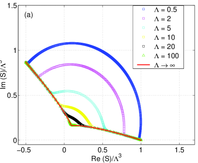
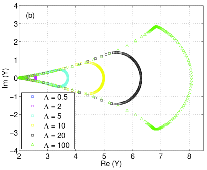
Figure 1:

(a) Argand diagram of the profiles of the gaugino condensate $S$ for $N=3$ and several values of $\Lambda$ in Model I. The continuous line represents the effective VY limit; (b) Argand diagram of the profiles of the $Y$ field for the same model and values of the parameters as before.

Let us first focus on the large $\Lambda$ case. The profile for $S$ is made out of two branches, $z>0$ and $z<0$. According to our theoretical analysis of Section 2, this configuration should be also described by an effective VY Lagrangian. In fact, we have checked that it can be obtained by solving the BPS equations for the VY Lagrangian with an appropriate prescription for the logarithm. In particular, the $z<0$ ($z>0$) branch is obtained using $\ln S^{N}=\ln(\Lambda^{3}R)^{N}+Ni\arg(S)\;(-2\pi i)$. The profile for $Y$ can be divided in three regions. The central one corresponds to the core, where $S$ remains almost constant but $Y$ changes very quickly, as can be seen in Figs 2. Notice that the width of this core goes to zero when we increase $\Lambda$. Moreover, the $Y$ profile can be calculated from the $S$ one. This is because, as expected in this limit, the condition ${\mathcal{W}}_{Y}=0$ is satisfied almost everywhere (it is only violated in the region where the phase is forced to change almost in an abrupt way to connect the two $S$ branches, as can be seen in Fig. 2b).

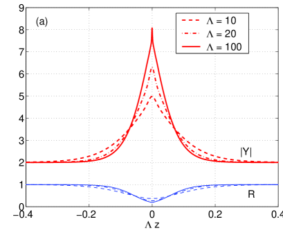
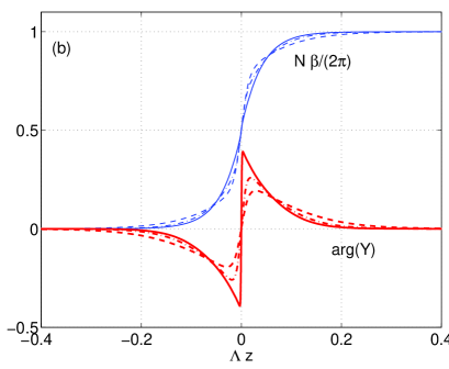
Figure 2:

(a) Profiles of $R$ (absolute value of $S$) and $|Y|$ as a function of $\Lambda z$ for $N=3$ and large values of $\Lambda$ in Model I (solid: $\Lambda=100$, dot-dashed: $\Lambda=20$, dashed: $\Lambda=10$); (b) profiles of $N\beta/(2\pi)$ and ${\rm arg}(Y)$ for the same model and values of the parameters as before.

In the small $\Lambda$ limit, the $Y$ field is frozen to its value at the minimum, $N\mp 1$ depending on the model we are considering (as can be clearly seen in Fig. 1b). We have checked that the profile for the $S$ field coincides with the corresponding BPS domain walls in the effective Landau–Ginzburg models of Eqs (17,20). This is illustrated in Figs 3, where we show both the absolute value $R$ (Fig. 3a) and the phase $\beta$ (Fig. 3b) of the $S$ field in Model I as a function of the rescaled position, $\Lambda z$, for small values of $\Lambda$, as well as its theoretical $\Lambda\rightarrow 0$ limit.

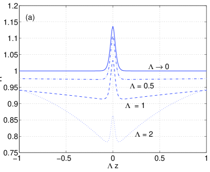
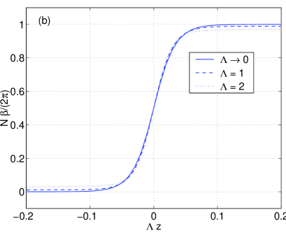
Figure 3:

(a) Profiles of $R$ (absolute value of $S$), as a function of $\Lambda z$, for $N=3$ and small values of $\Lambda$ (dotted: $\Lambda=2$, dashed: $\Lambda=1$, dot-dashed: $\Lambda=0.5$, solid: LG limit $\Lambda\rightarrow 0$) in Model I; (b) profiles of $N\beta/(2\pi$) for the same model and values of the parameters as before. The $\Lambda=0.5$ curve is not shown explicitly as it is indistinguishable from the LG limit on the graph.

We have therefore found a uniparametric family of BPS domain walls for the case $(N=3,k=1)$. The theory describing these walls interpolates between the super Yang–Mills Veneziano–Yankielowicz model (with some given rules about how to glue the different sectors of the potential) and a Landau–Ginzburg model. On the other side, we have also analyzed the $(N=3,k=2)$ case. There are no BPS domain walls with these boundary conditions (see Appendix B), in other words the domain wall connects the two vacua through the shortest path in $S$ space.

Let us now try to extend this result for higher values of $N$, where a richer pattern of domain walls is possible. Notice that BPS domain walls have to satisfy the constraint given by Eq. (27). This equation involves two fields which, in the limits explained before ($\Lambda\rightarrow\infty$ and $\Lambda\rightarrow 0$), should split into two simple -more restrictive- equations, since the dynamics are controlled only by one field. As we will see, the compatibility of these equations is the key to understanding the pattern of domain walls for arbitrary $N$ values.

3.2 General analysis: results

When considering domain walls in models with $N>3$, the possibility of having different types of walls, connecting the different vacua, arises. We first consider complex walls, which connect different vacua with $|S|=\Lambda^{3}$, and briefly discuss real walls (connecting the vacuum in Model II at $|S|=0$ to a vacuum at $|S|=\Lambda^{3}$) at the end of the section.

For the moment we shall exclude the cases where $k=N/2$ (with $N$ even). They correspond to $S(-\infty)=-S(\infty)$ and give a constraint that includes $S=0$ as a possible point in their trajectory, where we have seen that the two models we are considering (I and II) have radically different behaviour. For a detailed study of these cases the reader is referred to Appendix B.

In our numerical searches for both BPS and non-BPS solutions, we have found just one domain wall solution interpolating between two given vacua. Our conclusions from these results and from our analysis of the BPS constraint equations detailed below are that, for finite $\Lambda$,

• the domain walls found in Model I are BPS-saturated only for $k=1$;

• in Model II we have found BPS-saturated walls for any value of $k$ in the range $1\leq k<N/2$. This actually covers all possible situations given that, for any $N$, there is always a path with $k<N/2$ that links any two chirally asymmetric vacua.

These statements are proved in Appendix B by going to the limit $\Lambda\to 0$ and appealing to the continuity of the solutions as a function of $\Lambda$. Moreover they are illustrated in Figs 4 for $N=5$ and $k=2$, where we plot, in Fig. 4a, the Argand diagram for the superpotential Eq. (6) of Model I. As we can see the larger $\Lambda$ is, the more the curve tends to a straight line, which corresponds to a BPS-saturated solution. Therefore, it looks likely that, in the $\Lambda\rightarrow\infty$ (VY) limit, these domain walls of Model I will turn into BPS ones.

In Figs. 4b,c we turn to Model II and plot the profiles of the fields $R$ (Fig. 4b) and ${\rm Re}\;[Y]$ (Fig. 4c) as a function of $\Lambda z$, for several values of $\Lambda$. The behaviour of the different curves is very similar to that of the $N=3$, $k=1$ case plotted before, and we have also appended in Fig. 4b the effective $\Lambda\rightarrow 0$ (Landau–Ginzburg) and $\Lambda\rightarrow\infty$ (VY) limits, which we shall discuss in a moment.

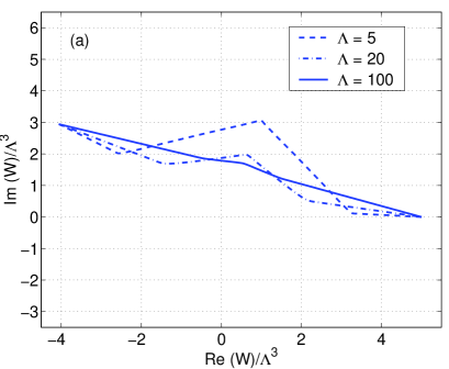
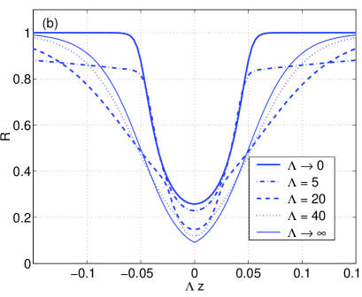
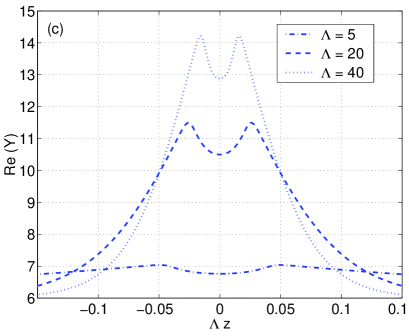
Figure 4:

(a) Argand diagram of ${\cal W}$ in Model I, $N=5$, $k=2$ for different values of $\Lambda$ (solid: $\Lambda=100$, dot-dashed: $\Lambda=20$, dashed: $\Lambda=5$); (b) profiles of $R$ (absolute value of $S$) as a function of $\Lambda z$ for $N=5$, $k=2$ and different values of $\Lambda$ in Model II (dot-dashed: $\Lambda=5$, dashed: $\Lambda=20$, dotted: $\Lambda=40$). The two limits are also plotted: VY $\Lambda\rightarrow\infty$ (thin solid) and LG $\Lambda\rightarrow 0$ (thick solid); (c) Profiles of ${\rm Re}\;[Y]$ as a function of $\Lambda z$ for the same model and values of the parameters as before.

Therefore we have seen that the pattern of domain walls for $k>1$ is totally different in Models I and II, although it looks like both are able to give BPS-saturated domain walls in the VY effective limit. In order to clarify this point further let us turn to the study of the constraint equation, Eq. (27).

Let us consider the walls connecting the vacua labelled by integers $a$ and $a+k$ (i.e. $S(+\infty)=S(-\infty)e^{i{2\pi k}/{N}}$). Using the parametrization of Eq. (LABEL:param), the constraint function for Model I is given by

$$C_{\rm I}(S,Y) = R^{1-N}e^{-{\rm Re}\;[Y]+N-1}\cos\left[(1-N)\beta-\frac{\pi k}{N}-{\rm Im}\;[Y]\right]$$ (29)

$$+ R\;{\rm Re}\;[Y]\,\cos\left(\beta-\frac{\pi k}{N}\right)-R\;{\rm Im}\;[Y]\,\sin\left(\beta-\frac{\pi k}{N}\right)-N\cos\left(\frac{\pi k}{N}\right)\;\;,$$

and, for Model II,

$$C_{\rm II}(S,Y) = R^{N+1}e^{{\rm Re}\;[Y]-N-1}\cos\left[(N+1)\beta-\frac{\pi k}{N}+{\rm Im}\;[Y]\right]$$ (30)

$$- R\;{\rm Re}\;[Y]\,\cos\left(\beta-\frac{\pi k}{N}\right)+R\;{\rm Im}\;[Y]\,\sin\left(\beta-\frac{\pi k}{N}\right)+N\cos\left(\frac{\pi k}{N}\right)\;\;.$$

The full constraint equations Eqs (29,30) are too complicated to study in general, but we can still gain some information about how the solutions interpolate between domain walls in the Landau–Ginzburg models and the VY limit by studying the corresponding constraint equations at $z=0$.

We are considering symmetric walls therefore, at the origin, $\beta_{0}=\pi k/N$ and ${\rm Im}\;[Y_{0}]$ = 0, where we use the subscript 0 to denote fields evaluated at $z=0$. For Model I the constraint equation takes the form

$$C_{\rm I}(R_{0},Y_{0})\equiv R_{0}^{1-N}e^{-Y_{0}+N-1}(-1)^{k}+R_{0}\,Y_{0}-N\cos\left(\frac{\pi k}{N}\right)=0\;\;,$$ (31)

and, for Model II,

$$C_{\rm II}(R_{0},Y_{0})\equiv R_{0}^{N+1}e^{Y_{0}-N-1}(-1)^{k}-R_{0}\,Y_{0}+N\cos\left(\frac{\pi k}{N}\right)=0\;\;.$$ (32)

In these equations $Y_{0}$ is real.

We can now plot the relationship between $R_{0}$ and $Y_{0}$ for both models, as a function of $N$ and $k$. Falling on the constraint curve is necessary, but not sufficient, for the existence of a BPS solution. Figure 5 shows the curve given by Eq. (31) for $N=5$ and $k=1$ (a) and $k=2$ (b), and that given by by Eq. (32) for $N=5$ and $k=1$ (c) and $k=2$ (d). The horizontal lines represent the value of $Y_{0}$ for which the corresponding Landau–Ginzburg ($\Lambda\rightarrow 0$) limit is reached ($Y_{0}=N-1$ in the first two plots and $Y_{0}=N+1$ in the last two). Note that, in all but Fig. 5b, the constraint equation intersects the $\Lambda\rightarrow 0$ horizontal line at either one (Figs 5a,c) or two (Fig. 5d) points. The intersection at larger $R_{0}$ for Model II ($N=5$, $k=2$) does not in fact correspond to a BPS wall, as is shown in Appendix B.

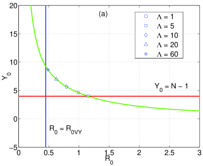
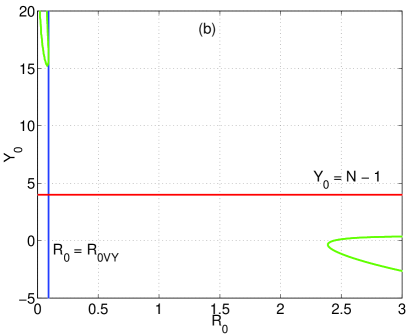
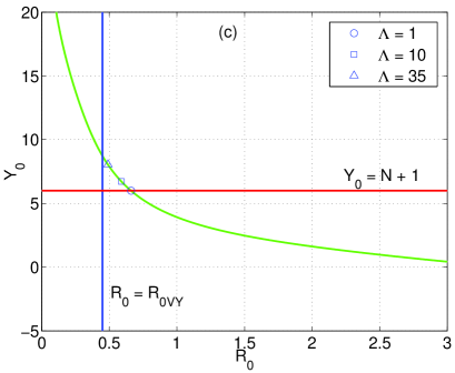
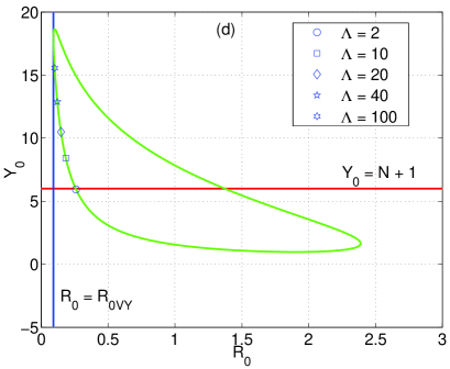
Figure 5:

(a) Contour plot of the constraint equation at $z=0$ as a function of $R_{0}$ and $Y_{0}$ (which is real) for $N=5$ and $k=1$ in Model I; (b) same for $k=2$; (c) same for Model II, $k=1$; (d) same for Model II, $k=2$. The horizontal lines represent the corresponding values for $Y_{0}$ at the LG ($\Lambda\rightarrow 0$) limit, whereas the vertical ones represent the values of $R_{0}$ in the VY ($\Lambda\rightarrow\infty$) one. The annotated symbols indicate the BPS-saturated solutions found in each case.

Let us consider now the VY (large $\Lambda$) limit, where the dynamics near the minima are governed by the light field, $S$. The $Y$ field just follows the evolution of the $S$ field, as dictated by the ${\mathcal{W}}_{Y}=0$ condition, $Y=N\mp 1-\ln({S^{N}}/{\Lambda^{3N}})$, with the minus (plus) sign taken for Model I (Model II). However, this condition must be violated in a region near $z=0$, as it is not consistent with ${\rm Im}\;[Y_{0}]=0$, $\beta_{0}=\pi k/N$. We denote the width of the region by $\Delta$, such that (with a suitable choice of the branch of the logarithm)

$$\begin{array}[]{ccccc}Y&=&\displaystyle N\mp 1-\ln\frac{S^{N}}{\Lambda^{3N}}\phantom{+i2\pi k}&&z<-\Delta\;\;,\\ &&\\ Y&=&\displaystyle N\mp 1-\ln\frac{S^{N}}{\Lambda^{3N}}+i\,2\pi k&&z>\Delta\;\;.\end{array}$$

As we will see, in that region $R$ is approximately constant but ${\rm Im}\;[Y]+N\beta$ changes very quickly to connect the two ${\mathcal{W}}_{Y}=0$ branches. We would expect the width of the region to be governed by the larger of the two masses in the theory, given in Eqs (LABEL:e:m2largeL), in which case it vanishes as $\Lambda^{-3}$ in the limit $\Lambda\to\infty$.

In this limit, and using Eqs (LABEL:VYlimit), the constraint equation becomes,

$$R_{0}(1-\ln R_{0})=\cos\left(\frac{\pi k}{N}\right)\;\;.$$ (33)

This equation has two solutions, one with $R_{0}<1$, and the other with $R_{0}>1$. Our analysis in Appendix B shows that there is, at most, only one BPS wall for finite $\Lambda$, and that it must be the solution with smaller $R_{0}$. It follows that, in the $\Lambda\to\infty$ limit, only one of these solutions to Eq. (33) corresponds to a domain wall, which is represented in Figs 5 by a vertical line, and denoted by $R_{0VY}$. Note also that the equation is identical to that obtained in Ref. [11] for the effective VY limit, with $k$ replaced by $N_{f}$, the number of matter flavours introduced in that case to study the model in its Higgs phase. There the effective VY limit was obtained when $m\rightarrow\infty$, with $m$ the mass of the matter condensates. Again, in that case, only the solutions with $N_{f}/N<1/2$ (i.e. $R_{0}<1$) would yield meaningful domain wall profiles, placing a restriction on the amount of matter one could consider. Here, as we mentioned before, the fact that it is only possible to define the effective VY limit for $k<N/2$ does not prevent us from building domain walls between any two neighbours (with the exception of $N$ even, $k=N/2$).

Once we have defined the effective VY limit, let us go back to the discussion of our results, for which we focus again on Figs 5. It is noticeable how, in all but Fig. 5b, not only do the constraint curves intersect the Landau–Ginzburg ($\Lambda\rightarrow 0$) limit, but also they connect continuously both the Landau–Ginzburg and VY ($\Lambda\rightarrow\infty$) limits. These are precisely the curves along which we have found BPS-saturated solutions at finite $\Lambda$, which are indicated by the annotated symbols, whereas the absence of such solutions is obvious in Fig. 5b, where the constraint curve does not connect the two limits. There is, therefore, a straightforward criterion to decide whether a particular model would yield BPS-saturated solutions for finite $\Lambda$, and that is given by the fact that the corresponding constraint equation interpolates continuously between the two existing limits. In the particular case of Fig. 5d, where there are actually two branches of the constraint equation that link the VY and Landau–Ginzburg limits, it is shown in Appendix B that only one of them gives BPS domain wall solutions. It is further shown, in that same Appendix, that the shape of the constraint curves illustrated for $N=5$ and $k=1,2$ in Figs 5 are examples of generic classes distinguished by $k<N/2$ and $k$ even or odd, and hence that our statements about the number of BPS solutions in the two models can be extended to all $N$, $k$.

Finally, as mentioned at the beginning of the section, there is the possibility, in Model II, of constructing so-called real domain walls, which interpolate between the chirally symmetric vacuum at ($|S|=0$, $Y=0$), and one of the $N$ vacua with $|S|=\Lambda^{3}$, $Y=N+1$. Although the chiral vacuum is certainly a supersymmetric minimum of the theory, in the sense that the scalar potential vanishes there, the Kähler potential (7) gives a metric which is singular at that point, so the status of the chirally symmetric vacuum is ambiguous. Nevertheless we have verified numerically that solutions exist in the model for our choice of Kähler metric.

4 Discussion, physical motivation, relation to previous work

Once we have shown that both these two Landau–Ginzburg models admit domain walls, and also have a well-defined effective VY limit when $\Lambda\rightarrow\infty$, we can proceed to discuss what the possible physical meaning of the extra $Y$ field should be. It was already pointed out years ago that the VY approach to SUSY QCD was neglecting degrees of freedom which would be as relevant as the gaugino condensate upon which the VY approach was developed. For example, spin zero glueballs which, in principle, should not be heavier than gluino condensates do not contribute to that effective action. Therefore it would be justified to attempt a different construction which would embed the VY model. This was done in Ref. [21] by introducing a real tensor superfield $U$ which contained gluino-gluino, gluino-gluon and gluon-gluon bound states, and a new $U$-dependent term to extend the VY effective action. Therefore this approach preserves the original logarithm and we do not believe that it could be directly compared to our Models I and II.

As was already mentioned in the introduction, the problems associated with the presence of the logarithm in the original VY model were addressed in Ref. [5] in the context of the linear multiplet formalism. In that case the authors were focusing on the study of gaugino condensation in the presence of a field dependent coupling, which brings into the theory a new scalar field whose vacuum expectation value induces the gauge coupling. By studying and proving the duality between the linear and chiral formulations of the problem, they were able to amend the VY chiral potential in order to eliminate ambiguities coming from the imaginary part of the gaugino condensate field ($u$ in that case). Again, we have not been able to find a direct link between this approach and ours of extending the theory by introducing a second field $Y$ but, nevertheless, we believe that exploring and constructing domain walls in this now unambiguous formulation would be a very interesting exercise.

On the other hand, our $Y$ field certainly has the form of a field dependent coupling, as the effective action contains $YS|_{F}$. If we accept that $Y$ is a coupling field, then it is tempting to interpret the extra piece, proportional to $e^{\pm Y}$, as the leading term of an instanton-induced contribution.

Finally we can comment about the different applications of BPS domain walls in the context of string theory. According to ’t Hooft’s conjecture [22], large-$N$ gauge theories should exhibit a phase described by perturbative strings. It is also believed [15] that, in this limit, BPS-saturated domain walls are effectively branes on which the QCD string can end. Triggered by this, much work has been devoted to studying the connection between domain walls and branes in recent years. For example a construction of BPS domain walls was carried out in Ref. [8] by exploiting the similarity of the super QCD Lagrangian (understanding by this the VY model amended to restore the $Z_{N}$ symmetry [7]) with that of the $A_{N}$ Landau–Ginzburg model, in the large-$N$ limit and for walls connecting adjacent vacua. In fact, there it was even attempted to identify the field content of this super QCD Lagrangian with those fields appearing in the supersymmetric formulation of the membrane action.

There has been also a lot of work on branes and strings at conifold singularities. Different dualities are supposed to be related to a transition in the geometry. This has been recently suggested by Vafa [16] in the Chern–Simons/topological strings duality framework. He considers Type IIA strings in a non-compact Calabi–Yau (CY) 3-fold geometry that includes a conifold and adds $N$ D6-branes wrapped over the ${\cal S}^{3}$ in the complex deformed conifold. That generates a ${\cal N}=1$ supersymmetric ${\rm SU}(N)$ theory. The relevant chiral superfields are $S$, proportional to the one defined in Eq. (5), and a new chiral field, $Y$, whose lowest component is given by the volume of the ${\cal S}^{3}$ (real part) and by the vev of some 3-form (imaginary part) that will play the role of $\theta$ angle. At lowest order, the superpotential is given by ${\mathcal{W}}=SY$ . The new field, Y, triggers the non-perturbative effects. Vafa proposes the following corrected superpotential

$$W=\frac{1}{\lambda}_{s}SY+iN^{2}e^{-Y/N}\;\;,$$ (34)

where $\lambda_{s}$ is the string coupling . If we integrate out the $Y$ field, by using ${\mathcal{W}}_{Y}=0$, we end up with the VY superpotential for the condensate. Notice that this superpotential shares two properties with our models: there is a linear, $SY$, term and an exponential term involving the new field, $Y$. The combination of these two facts gives the logarithmic dependence in the effective Lagrangian describing the gaugino bilinear. Therefore we believe that our models could shed some light on the role played by the fields that couple to the gaugino condensate. These fields are very important if we want to understand the core of the domain wall.

5 The large-$N$ limit

We have seen in the previous examples how to calculate BPS domain walls for the VY Lagrangian in the cases where they exist in the extended theory. Let us assume that the complete theory supports these BPS domain walls. Now we can study how they behave for large values of $N$ (see also Refs [8, 24, 23]). This is particularly important because, in that limit, these domain walls are thought to be the field theory realization of branes.

We want to solve the BPS equation

$${\cal K}_{S\bar{S}}\partial_{z}\bar{S}=e^{i\gamma}\ln\frac{S^{N}}{\Lambda^{3N}}\;\;,$$ (35)

for the $(N,k)$ case (i.e. $\gamma=\pi/2-\pi k/N$), and large $N$ values. In order to do that, it is useful to define the parameter $\epsilon=\frac{k\pi}{N}$. Then the constraint for $R_{0}$, Eq. (33), becomes

$$\cos\epsilon-R_{0}\,(1-\ln R_{0})=0\;\;.$$ (36)

Notice that the allowed values of $k$ will depend on the details of the theory that generalizes the VY Lagrangian. For example, in Model I only $k=1$ will be allowed, whereas in Model II we can consider any value of $k$. In any case, assuming $k\ll N$, we can expand $R_{0}$ in terms of $\epsilon$ to obtain its large-$N$ limit

$$R_{0}=1\pm\epsilon+\frac{\epsilon^{2}}{6}+{\cal O}(\epsilon^{3})\;\;.$$ (37)

Then $|S|$ deviates from its value at the minima by ${\cal O}(\epsilon)$. Since the phase of the condensate is also ${\cal O}(\epsilon)$, we will adopt the following parametrization

$$S(z)=\Lambda^{3}(1-\epsilon\rho(z))\,e^{i\epsilon\psi(z)}\;\;,$$ (38)

with $\rho(z),\psi(z)$ real functions of ${\cal O}(1)$. Substituting the previous expression into the BPS equation, Eq. (35), we get

$$\rho(z) = e^{9z/\Gamma}+(e^{9z/\Gamma}-\frac{7}{6}e^{18z/\Gamma})\epsilon+{\cal O}(\epsilon^{2})\;\;,$$

$$\psi(z) = e^{9z/\Gamma}+{\cal O}(\epsilon^{2})\;\;,$$

for the $z<0$ branch (and the ‘symmetric’ one in the $z>0$ branch). In these equations $\Gamma=\frac{1}{\Lambda N}$ fixes the domain wall width. In order to determine the $N$ dependence of the relevant quantities (i.e. width and tension of the wall) in the large-$N$ limit, it is standard to rescale the fields so that the Lagrangian scales like $N$. For example, Eq. (1) will appear as

$$\langle\lambda\lambda\rangle_{k}\equiv\langle{\rm Tr}\lambda^{a}\lambda_{a}\rangle_{k}=N{\tilde{\Lambda}}^{3}e^{i\frac{2\pi}{N}k}\;\;.$$ (40)

If we calculate now the domain wall tension when interpolating from vacuum $a$ to vacuum $a+k$ we get

$$\sigma=|W_{a+k}-W_{a}|=N^{2}{\tilde{\Lambda}}^{3}2\sin\epsilon\;\;,$$ (41)

i.e. for $k={\cal O}(1)$ the tension is expected to scale as $N$. Notice that there are two different ways to calculate the domain wall energy: using the two-field theory or the effective VY one. The validity of Eq. (41) relies on the differentiability of the domain wall profile, so it can be only used in the two field theory. In the VY model, one should split the energy into the contributions coming from the $z<0$ and $z>0$ branches. In that case we get

$$\sigma_{VY}=N^{2}{\tilde{\Lambda}}^{3}2|\sin\epsilon-\epsilon R_{0}|\;\;.$$ (42)

This result coincides with the one obtained by using squark matter fields (see Ref. [14]) as the extra fields providing regular domain walls. This is due to the fact that, in both cases, the same prescription is used to calculate the imaginary part of the logarithm. We have seen how this prescription naturally emerges when integrating out the $Y$ field (see Eq. (LABEL:VYlimit)), as it was also shown in Ref. [11] for the squark matter fields. Notice, however, that for $k>1$ the squark fields, as described by the TVY Lagrangian, do not provide regular BPS domain walls for high enough values of their masses. This means that, in these cases, the extra fields that enter the logarithmic term in the effective potential can not be ignored. They play a relevant role and are excited in the subcore of the domain wall.

On the other hand, the difference between $\sigma$ and $\sigma_{VY}$ gives us information about the energy that is stored in the $Y$ subcore, i.e. the spatial region in the large $\Lambda$ limit where the phase of $Y$ changes quickly. Since $\sigma\sim{\tilde{\Lambda}}^{3}N$ and $\sigma_{VY}\sim{\tilde{\Lambda}}^{3}$, we conclude (as first shown in Ref. [14]) that, in the large-$N$ limit, most of the energy concentrates in this subcore.

6 Conclusions

We have studied the existence of BPS-saturated domain walls in two extensions of the Veneziano–Yankielowicz effective Lagrangian formulation in order to study SUSY Yang–Mills theories. These are motivated by the existence of several problems associated with the presence of a logarithm of the gaugino condensate field in the effective potential of the VY formulation, which causes ambiguities when studying dynamical questions such as the formation of domain walls. Our extensions, which we denote as of the Landau–Ginzburg type, avoid such problems by introducing an extra chiral superfield, $Y$, and a logarithm-free interaction which, in the limit of heavy $Y$, result in the effective VY model. Within this framework we have constructed domain walls which turn out to be BPS-saturated in one of the models but not in the other one. In any case, both seem to give BPS-saturated walls in the effective VY limit.

We have also studied the limit of light $Y$ field, in which the models proposed approach Landau–Ginzburg models with which one can construct well-defined BPS-saturated walls. It turns out that it is possible to define a criterion to decide whether our particular extensions of VY admit BPS-saturated walls at any point in between the two (VY and LG) limits: this is given by whether the BPS constraint, associated with the corresponding BPS equations, is able to interpolate continuously between both limits. Our results can be proven to hold for any values of $N$ (number of colours) and $k$ (neighbours between which we interpolate).

Finally we comment on the possible physical significance of the extra field $Y$, and the connection of our approach with other proposed models existing in the literature. Although there is no direct evidence so far, the similarity of this model with some domain wall constructions done in the context of string theory is quite remarkable, and it deserves further investigation.

Appendix A The Newton method for finding solutions

The numerical solutions to the field equations were found with Newton’s method, also called the Newton-Raphson method (NR). This was implemented by a Fortran 90 program.

We wish to find extremal energy configurations for the discretized energy functional of the domain wall, $E(f_{A})$, where $f_{A}$ denote the degrees of freedom: here, the values of the complex fields and their conjugates at each point on the lattice.

The Newton-Raphson algorithm consists of iterating the update

$$df_{A}=-\left(\frac{{d^{2}}E}{{df_{A}}{df_{B}}}(f)\right)^{-1}\frac{dE}{df_{B}}(f)\;\;.$$ (43)

In order to solve the matrix equation (43) our program calls linear algebra routines zgbtrf and zgbtrs from the Silicon Graphics implementation of the BLAS library.

It is necessary to use a rescaled lattice because of the presence of widely differing mass scales when $\Lambda$ differs from $O(1)$. The rescaling used takes the form

$$s=\frac{1}{2}(\tanh({m_{1}}{x})+\tanh({m_{2}}{x}))\;\;,$$ (44)

where $x$ is the physical position, $s$ is the rescaled position and $(m_{1},m_{2})$ are parameters chosen to give the best spread of lattice points. There should be enough points in the central region to accurately follow the rapidly changing fields, while the total number of points should be minimized so that the program takes less time to run.

Once the rescaling is chosen the lattice points are placed equally spread in $s$ between $s=-1$ and $s=1$. This means that the end points of the lattice are at spatial infinity.

The number of lattice points used was typically between 100 and 300, and the number of iterations needed to reach convergence was between 20 and 1000.

Spatial derivatives are calculated three ways, with forward, backward and symmetric derivatives. The energy function $E(f_{i})$ has contributions from all three forms of the derivative, added with equal weighting. The advantage of this approach is that symmetry between left and right is maintained, while odd and even numbered points are kept in close contact, which would not be the case were only symmetric derivatives used.

The values of the fields on the boundaries are set equal to their vacuum values, and are kept fixed. The walls are symmetrical between left and right, because of the $Z_{N}$ symmetry in the Lagrangian. This links the field values in one half of the wall with the conjugates of the values in the other half, i.e.

$$S(s)=\bar{S}(-s)e^{i2\pi k/N},\quad Y(s)=\bar{Y}(-s)\;\;.$$ (45)

However, rather than model half of the wall, it was decided to model both sides, because of the difficulty of establishing simple boundary conditions at $z=0$, consistent with the strategy of programming with complex, rather than real, fields.

The convergence criterion was framed in terms of $c=\sum_{A}\left|dE/df_{A}\right|$. The algorithm is judged to have converged when $c$ reaches $\mathrel{\mathchoice{\lower 0.5pt\vbox{\halign{$\math\displaystyle\hfil#\hfil$\cr\scriptstyle<\crcr{\scriptstyle\sim}\crcr}}}{\lower 0.5pt\vbox{\halign{$\math\textstyle\hfil#\hfil$\cr\scriptstyle<\crcr{\scriptstyle\sim}\crcr}}}{\lower 0.5pt\vbox{\halign{$\math\scriptstyle\hfil#\hfil$\cr\scriptstyle<\crcr{\scriptstyle\sim}\crcr}}}{\lower 0.5pt\vbox{\halign{$\math\scriptscriptstyle\hfil#\hfil$\cr\scriptstyle<\crcr{\scriptstyle\sim}\crcr}}}}10^{-10}$.

When far from a solution the size of the update may have to be reduced. It is guaranteed that, for a sufficiently small movement, following $-df_{A}$ will approach a solution. However, a full NR update may overshoot, and lead to divergent field values, rather than converging. To deal with this, in the initial stages of a run the size of the update is reduced by a factor of 10, or even 100. Systematic methods of doing this, such as backtracking along $df_{A}$, were judged to be unnecessary.

To check the BPS saturation of a solution two criteria are used. Firstly, the total energy of the wall is compared to the BPS energy, which is itself easily calculated. Because of discretisation error, the numerically determined energy is usually below the true BPS value.

The second method of determining whether solutions are BPS is to check that the wall follows a straight line in $W$-space. The straightness of the line is quantified by the ratio of the maximum deviation from a straight line linking the ends, divided by the length of the line. If this quantity can be shown to decrease towards zero as the number of lattice points is increased, the configuration is taken to be BPS.

Appendix B Detailed analysis of the BPS constraint equations

In this Appendix we supply details of the analysis behind Section 3, where we described the values of $N$ and $k$ admitting BPS domain walls.

In Appendix B.1 we study the limit $\Lambda\to 0$, where our models tend to the Landau–Ginzburg models LG1 and LG2 described in Section 2. In this limit we are able to prove exact results giving the values of $(N,k)$ for which BPS walls exist and, conversely, those for which BPS walls do not exist. Our argument uses continuity in $\Lambda$ to make the statement that BPS walls cannot exist in a particular model at $\Lambda>0$ if its $z=0$ constraint curve, Eqs. (31, 32), reaches the LG limit at a point where we know there is no BPS domain wall.

To this end, we must analyse the $z=0$ curves, to enumerate all possible BPS domain wall solutions, and to check that they have an LG limit. This is done in Appendix B.2.

B.1 Analysis in the Landau–Ginzburg limit

In the Landau–Ginzburg limit, $\Lambda\to 0$, the extra field $Y$ stays at its vacuum value $Y_{*}=N\mp 1$. We require that solutions of the constraint equations Eqs (29,30) exist for all $\beta$ in the range $0\leq\beta\leq 2\pi k/N$, and asymptote to $R=1$ at $\beta=0$ and $\beta=2\pi k/N$. Any solution to the constraint equation at $z=0$ which does not connect the vacua is a ‘fake’ solution and cannot represent a BPS domain wall. By continuity in $\Lambda$, solutions to the full constraint equation for our interpolating models which tend to these fake solutions as $\Lambda\to 0$ are also inadmissable as BPS walls.

Firstly, consider the Model I constraint equation Eq. (29), and define a new angle $\delta=\beta-\pi k/N$, so that the constraint function becomes

$$C_{LG1}(R,\delta)=R^{1-N}\cos[(N-1)\delta](-1)^{k}+(N-1)R\cos\delta-N\cos\left(\frac{\pi k}{N}\right)\;\;.$$ (46)

Where $\cos[(N-1)\delta](-1)^{k}>0$, the constraint function has a single minimum as a function of $R$ at $R=R_{\rm min}$. One can show that as one varies $\delta$, the maximum value of this minimum occurs at $\delta_{{\rm max},m}=\pi m/N$, with $-k\leq m\leq k$, and $m$ even (odd) when $k$ is even (odd). At these saddle points

$$C_{LG1}(R_{\rm min},\delta_{{\rm max},m})=N\left(\cos\left(\frac{\pi m}{N}\right)-\cos\left(\frac{\pi k}{N}\right)\right)\;\;.$$ (47)

When this is greater than zero there can be no solutions to $C_{LG1}(R,\delta)=0$. For $k>1$, there is always a value of $m$ for which $C_{LG1}(R_{\rm min},\delta_{{\rm max},m})>0$, and so the constraint curve cannot move continuously between $\delta=0$ and $\delta=\pi k/N$.

Hence we conclude there are no BPS domain walls in the Landau–Ginzburg limit ($\Lambda\to 0$) of Model I for any $k>1$, and only one for $k=1$

For the Landau–Ginzburg limit of Model II, we can rewrite the constraint function as

$$C_{LG2}(R,\delta)=R^{N+1}\cos[(N+1)\delta](-1)^{k}-(N+1)R\cos\delta+N\cos\left(\frac{\pi k}{N}\right)\;\;.$$ (48)

Where $\cos[(N+1)\delta](-1)^{k}>0$ the constraint function has a single minimum at $R=R_{\rm min}$. One can again show that the maximum value of this minimum occurs at $R_{\rm min}=1$, $\delta_{{\rm max},m}=\pi m/N$, with $-k\leq m\leq k$, and $m$ even (odd) when $k$ is even (odd). At these saddle points

$$C_{LG2}(R_{\rm min},\delta_{\rm max})=N\left(\cos\left(\frac{\pi k}{N}\right)-\cos\left(\frac{\pi m}{N}\right)\right)\;\;.$$ (49)

In this case, the value of the constraint function at the saddles is always less than zero (unless $m=k$), and therefore there are two solutions to the equation $C_{LG2}=0$ when $\cos(\pi k/N)\geq 0$, and only one if $\cos(\pi k/N)<0$. Where $\cos[(N+1)\delta](-1)^{k}<0$, the constraint function becomes a monotonically decreasing function of $R$. For these values of $\delta$ there can only be one solution to the constraint equation for $\cos(\pi k/N)\geq 0$, and none for $\cos(\pi k/N)<0$. Hence only one of the solutions to the constraint equation at $\delta=0$ (which one can straightforwardly see is the one with smaller $R$) can connect two vacua for $\cos(\pi k/N)\geq 0$, and none for $\cos(\pi k/N)<0$.

In fact, we can also eliminate the solution at $R=0$ for $\cos(\pi k/N)=0$, as it cannot interpolate between vacua with $R=1$.

Hence we conclude there are no BPS domain walls in the Landau–Ginzburg limit ($\Lambda\to 0$) of Model II for any $k\geq N/2$, and only one for $k<N/2$

B.2 Analysis of constraint curves at $z=0$

In this Appendix we show that the constraint curves at $z=0$ fall into a small number of classes: four if $N$ is odd, and six if $N$ is even. These classes are distinguished by having the same number of intercepts with the lines representing the LG and VY limits, and by having the same number of points at which they are either horizontal or vertical. This classification helps us to be certain that we have found all possible types of BPS wall solution in Section 3.

Firstly we note that, as $k$ is an integer, $\cos(k\pi)$ can only have the values $1$ or $-1$ and, if $N$ is odd, $\cos(k\pi/N)$ can be either positive or negative. There are therefore four distinct cases for which we can expect the constraint curve to be qualitatively different. If $N$ is even, $\cos(k\pi/N)$ can be zero, and there are therefore six classes.

We have already eliminated $\cos(\pi k/N)\leq 0$ from consideration in the Landau–Ginzburg limits of both models, and thus we need concentrate only on the cases $\cos\pi k=\pm 1$, with $\cos(\pi k/N)>0$ For illustration purposes it is therefore sufficient to consider, as we have done, $N=5$ with $k=1,2$ only.

We look for intercepts with four particular curves, namely

$$R_{0} = 1\;,$$ (50)

$$Y_{0} = 0\;,$$ (51)

$$Y_{0} = N\mp 1\;,$$ (52)

$$Y_{0} = N\mp 1-N\ln R_{0}\;,$$ (53)

with the negative sign taken for Model I and the positive sign for Model II. Note that the third of these is the LG limit, and the fourth is the VY limit in the case of even $k$. Along these curves the constraint equations are sufficiently simple that the number of solutions can easily be deduced.

The other information we use is the slope of the constraint curves

$$\frac{\partial Y_{0}}{\partial R_{0}}=\left\{\begin{array}[]{cr}\displaystyle-\frac{(N-1)R_{0}^{-N}e^{-Y_{0}+N-1}(-1)^{k}-Y_{0}}{R_{0}(R_{0}^{-N}e^{-Y_{0}+N-1}(-1)^{k}-1)}&\textrm{Model I}\\[15.0pt] \displaystyle-\frac{(N+1)R_{0}^{N}e^{Y_{0}-N-1}(-1)^{k}-Y_{0}}{R_{0}(R_{0}^{N}e^{Y_{0}-N-1}(-1)^{k}-1)}&\textrm{Model II}\end{array}\right.$$ (54)

By noting the sign of $\partial Y_{0}/\partial R_{0}$ we can trace the shape of the curve. Note that for even $k$ the constraint curve is vertical at $Y_{0}=N\mp 1-N\ln R_{0}$, which is precisely at the VY limit. This is illustrated in Figs 5b and 5d, where it can be verified that the constraint curves are vertical at $R_{0}=R_{0VY}$.

Now we shall consider the two cases ($k$ even or odd) in detail, in Model I.

When $k$ is even (see Fig 5b), Eqs. (50,52) can not be satisfied, so the constraint curve never crosses the lines $R_{0}=1$, $Y_{0}=N\mp 1$. However, it does cross Eq. (51) once at $R_{0}>0$ and Eq. (53) twice, once on either side of $R_{0}=1$.

Let us trace the curve from its $R_{0}<1$ intercept with Eq. (53). For the part of the curve with $Y_{0}>N-1-N\ln R_{0}$, the slope is negative, and so the curve must move left and up. The part with $Y_{0}<N-1-N\ln R_{0}$ has positive slope but, because it cannot cross $Y_{0}=N-1$, it must reach a turning point, and also move left and up. This accounts for the upper branch of the curve in Fig. 5b.

Starting now from the $R_{0}>1$ intercept with Eq. (53), the lower part of the curve will follow $R_{0}\rightarrow\infty,Y_{0}\rightarrow-\infty$. The upper part will cross Eq. (51) and then $\partial Y_{0}/\partial R_{0}=0$ and so turn down again. It cannot cross Eq. (51) again, and so $Y_{0}\rightarrow 0$ from above, as $R_{0}\rightarrow\infty$.

When $k$ is odd, (Fig 5a), we can by inspection of Eq. (32) see that $C_{\rm I}(R_{0},Y_{0})=0$ only when $Y_{0}>0$. Furthermore Eqs. (50,52) can each be satisfied once, while Eq. (53) is never true: hence the curve is never vertical, and in fact the slope is always negative. This means that $Y_{0}\rightarrow 0$ from above as $R_{0}\rightarrow\infty$, while as $R_{0}\rightarrow 0$, $Y_{0}\rightarrow\infty$.

One can go through a similar analysis to satisfy oneself that the curves for Model II are similar to Figs. 5c, 5d. The principle differences between the models occur for even $k$ and can be seen by comparing Fig. 5b to Fig. 5d: Model I has no intercepts with $R_{0}=1$, while Model II has two. There are also no intercepts with $Y_{0}=N-1$ in Model I, but one can easily check that there are two with the analogous line $Y_{0}=N+1$ in Model II. The intercept with $R_{0}>1$ does not however correspond to a domain wall in the Landau–Ginzburg ($\Lambda\to 0$) limit, as was shown in Appendix B.1.

References

- [1] G. Dvali and M. Shifman, Phys. Lett. B396 (1997) 64; erratum ibid. B407 (1997) 452 [hep-th/9612128].
-
[2]
E. Witten, Nucl. Phys. B202 (1982) 253;
V. Novikov, M. Shifman, A. Vainshtein and V. Zakharov, Nucl. Phys. B229 (1983) 407;
I. Affleck, M. Dine and N. Seiberg, Nucl. Phys. B256 (1985) 557. - [3] G. Veneziano and S. Yankielowicz, Phys. Lett. 113B (1982) 231.
- [4] A. Kovner and M. Shifman, Phys. Rev. D56 (1997) 2396 [hep-th/9702174].
- [5] C. Burgess, J.P. Derendinger, F. Quevedo and M. Quirós, Phys. Lett. B348 (1995) 428 [hep-th/9501065].
- [6] I.I. Kogan, A. Kovner and M. Shifman, Phys. Rev. D57 (1998) 5195 [hep-th/9712046].
- [7] G. Gabadadze, Nucl. Phys. B544 (1999) 650 [hep-th/9808005].
- [8] G. Dvali, G. Gabadadze and Z. Kakushadze, Nucl. Phys. B562 (1999) 158 [hep-th/9901032].
- [9] T. Taylor, G. Veneziano and S. Yankielowicz, Nucl. Phys. B218 (1983) 493.
- [10] A.V. Smilga and A.I. Veselov, Phys. Rev. Lett. 79 (1997) 4529 [hep-th/9706217]; Nucl. Phys. B515 (1998) 163 [hep-th/9710123]; Phys. Lett. B428 (1998) 303 [hep-th/9801142].
- [11] B. de Carlos and J.M. Moreno, Phys. Rev. Lett. 83 (1999) 2120 [hep-th/9905165].
- [12] B. de Carlos, M. Hindmarsh, N. McNair and J.M. Moreno, [hep-th/0102033].
- [13] D. Binosi and T. ter Veldhuis, Phys. Rev. D63 (2001) 085016 [hep-th/0011113].
- [14] A.V. Smilga, [hep-th/0104195].
- [15] E. Witten, Nucl. Phys. B507 (1997) 658 [hep-th/9706109].
-
[16]
C. Vafa, [hep-th/0008142];
B. Acharya and C. Vafa, [hep-th/0103011]. -
[17]
V. Kaplunovsky, J. Sonnenschein and S. Yankielowicz,
Nucl. Phys. B552 (1999) 209 [hep-th/9811195];
Y. Artstein, V. S. Kaplunovsky and J. Sonnenschein, JHEP 0102 (2001) 040, [hep-th/0010241]. -
[18]
N. Dorey and S.P. Kumar, JHEP 002 (2000)
006 [hep-th/0001103];
A. Frey, JHEP 0012 (2000) 020 [hep-th/0007125];
C. Bachas, J. Hoppe and B. Pioline, [hep-th/0007067]. - [19] E.R.C. Abraham and P.K. Townsend, Nucl. Phys. B351 (1991) 313.
- [20] M. Cvetič, F. Quevedo and S.-J. Rey, Phys. Rev. Lett. 67 (1991) 1836.
- [21] G.R. Farrar, G. Gabadadze and M. Schwetz, Phys.Rev. D58 (1998) 015009 [hep-th/9711166].
- [22] G. ’t Hooft, Nucl. Phys. B72 (1974) 461.
- [23] G. Dvali and Z. Kakushadze, Nucl. Phys. B537 (1999) 297 [hep-th/9807140].
- [24] G. Gabadadze and M. Shifman, Phys. Rev. D61 (2000) 075014 [hep-th/9910050].