Field Decomposition and the Ground State Structure of SU(2) Yang-Mills Theory

Abstract

We compute the effective potential of SU(2) Yang-Mills theory using the background field method and the Faddeev-Niemi decomposition of the gauge fields. In particular, we find that the potential will depend on the values of two scalar fields in the decomposition and that its structure will give rise to a symmetry breaking.

Recently it has been proposed that the different phases of Yang-Mills theory can be described by an appropriate decomposition of the gauge fields [1]. This decomposition has been used to describe the long distance limit of Yang-Mills theory, where stable knotted solitons have been found [2]. Furthermore the decomposition leads to a Lagrangian with a manifest duality between the electric and magnetic variables [3].

Here we shall investigate the effective theory in terms of the variables of the decomposition. The result will be an alternative way to view the ground state structure of the theory. We find that the effective potential, at the one loop level of approximation, will lead to a non-trivial ground state which suggests that symmetry breaking and dimensional transmutation [4] takes place.

In order to determine the effective theory we rely on the formalism of Coleman and Weinberg [4] and we will use the background field method [6] to perform the calculations.

The classical action of SU(2) Yang-Mills theory is

$$S=-\frac{1}{4}\int d^{4}xF^{a}_{\mu\nu}F^{a\mu\nu}$$ (1)

where $F_{\mu\nu}^{a}=\partial_{\mu}A_{\nu}^{a}-\partial_{\nu}A_{\mu}^{a}+g\epsilon^{abc}A_{\mu}^{b}A_{\nu}^{c}$. Following [1][3] the off diagonal gauge fields are decomposed as follows.

$$A_{\mu}^{+}=A_{\mu}^{1}+iA_{\mu}^{2}=i\psi_{1}\mathbf{e}_{\mu}+i\psi_{2}\mathbf{e}_{\mu}^{*}$$ (2)

where

$$\mathbf{e}_{\mu}=\frac{1}{\sqrt{2}}(e_{\mu}^{1}+ie_{\mu}^{2})$$ (3)

with the normalisation condition

$$e_{\mu}^{a}e^{b\mu}=\delta^{ab}$$ (4)

$\psi_{1}$ and $\psi_{2}$ are complex scalar fields. The diagonal gauge field, $A_{\mu}^{3}$, remain intact. Here we are interested in implementing this decomposition in the one-loop effective Yang-Mills action [7][8]. For this we first use the background field method [6] to find the effective potential up to one-loop order and then introduce the change of variables as in (2). This will yield an effective potential dependent only on the scalar fields in the decomposition, which allows us to study the phase structure of the theory.

In order to implement the background field method we make the following shift of the gauge fields in the action

$$A_{\mu}^{a}\rightarrow A_{\mu}^{a}+\mathcal{A}_{\mu}^{a}$$ (5)

where we view $A_{\mu}^{a}$ as a classical background field. When quantising, using the path integral formulation, we integrate over $\mathcal{A}_{\mu}^{a}$ only. We shall find that making this shift corresponds to making the following shifts in the complex scalar fields

$$\psi_{1}\rightarrow f_{0}+\psi_{1}\quad\psi_{2}\rightarrow g_{0}+\psi_{2}\quad f_{0},g_{0}\in\mathbb{R}$$ (6)

where $f_{0}$ and $g_{0}$ are constants. This is due to the fact that the minima of the eventual potential should be translation invariant. Hence we conclude that the shifted off diagonal fields are

$$A_{\mu}^{1}=\frac{1}{\sqrt{2}}(g_{0}-f_{0})e_{\mu}^{2}\quad A_{\mu}^{2}=\frac{1}{\sqrt{2}}(f_{0}+g_{0})e_{\mu}^{1}$$ (7)

The effective potential is the negative sum of all non-derivative terms in the Lagrangian. We remove the derivatives in a covariant way, i.e. we also remove the background field $A_{\mu}^{3}$. At the tree level of Yang-Mills we have

$$V=\frac{g^{2}}{4}\epsilon^{abc}\epsilon^{aef}A_{\mu}^{b}A_{\nu}^{c}A^{\mu e}A^{\nu f}$$ (8)

This quantity is in general not gauge invariant. However it is invariant under constant gauge transformations, which is consistent with our expectation that the ground state of the theory should be translation invariant. Using the decomposition (7) we obtain

$$V=\frac{g^{2}}{8}(f_{0}^{2}-g_{0}^{2})^{2}$$ (9)

The minima of this potential is along the directions $f_{0}=\pm g_{0}$ where the potential is zero. The vacuum is infinitely degenerate and there is no symmetry breaking. In the following we are interested in locating the ground state of the theory by inspecting radiative corrections to (9).

The Lagrangian is invariant under gauge transformations of $\mathcal{A}_{\mu}^{a}$ and in order to compute the quantum corrections we fix the gauge. Here we will use the background field analogue of Feynman gauge, the Lagrangian with gauge fixing terms and ghosts is then

$$L = -\frac{1}{4}\left(\partial_{\mu}(A_{\nu}^{a}+\mathcal{A}_{\nu}^{a})-\partial_{\nu}(A_{\mu}^{a}+\mathcal{A}_{\mu}^{a})+g\epsilon^{abc}(A_{\mu}^{b}+\mathcal{A}_{\mu}^{b})(A_{\nu}^{c}+\mathcal{A}_{\nu}^{c})\right)^{2}$$ (10)

$$-\frac{1}{2\xi}\left((\partial_{\mu}\delta^{ab}+g\epsilon^{abc}A^{c}_{\mu})\mathcal{A}_{\mu}^{a}\right)^{2}-\bar{c}^{a}(\partial_{\mu}\delta^{ab}+g\epsilon^{abc}(A_{\mu}^{c}+\mathcal{A}_{\mu}^{c}))^{2}c^{c}$$

Where $\xi$ is the gauge fixing parameter, here $\xi=1$. The Lagrangian can be rewritten, keeping only terms quadratic in $\mathcal{A}_{\mu}^{a}$ and $c^{a}$, as follows

$$L = -\frac{1}{2}\mathcal{A}^{a\alpha}\left(-(D^{2})^{ac}g_{\alpha\beta}-2g\epsilon^{abc}F^{b}_{\alpha\beta}\right)\mathcal{A}^{c\beta}+\bar{c}^{a}(-(D^{2})^{ac})c^{c}$$ (11)

where $D_{\mu}^{ab}=\partial_{\mu}\delta^{ab}+g\epsilon^{abc}A_{\mu}^{c}$. We note here the gauge invariant structure of the differential operators with respect to background gauge transformations. The motivation for keeping quadratic terms only is that the linear terms disappear in the calculation process and higher powers than two in $\mathcal{A}_{\mu}^{a}$ do not contribute to the one-loop corrections.

The effective action, $S_{eff}$, in Euclidean space, is defined by

$$e^{S_{eff}} = \int[d\mathcal{A}][dc][d\bar{c}]\exp\left(\int d^{4}xL\right)$$ (12)

$$= \exp\left(\int d^{4}x(-\frac{1}{4}(F^{a}_{\mu\nu})^{2}+...)\right)(\mbox{det}\Delta_{gauge})^{-1/2}(\mbox{det}\Delta_{ghost})$$

We note that the result of the computation will be a renormalisation of the gauge coupling and the background field.

$$g\rightarrow Z_{g}g\quad A_{\mu}\rightarrow Z_{A}^{1/2}A_{\mu}$$ (13)

Also the gauge fixing parameter, $\xi$, is renormalised but that we need not consider when computing one-loop corrections. Gauge invariance dictates that $Z_{g}=Z_{A}^{-1/2}$ [6] so that the effective Lagrangian will look like

$$L_{eff}=-\frac{1}{4}Z_{A}F_{\mu\nu}^{a}F^{a\mu\nu}+\mbox{higher order terms}$$ (14)

To compute the functional determinants in (12) the proper time method [14] is often used. See for example [9], [8] and [10]. Here we will however use a different method, similar to [4] and [11]. We feel this method might simplify our computations here.

Computing the functional determinants in equation (12) corresponds to computing the Feynman diagrams in figure 1 and the corresponding ghost diagrams.

Figure 1: The types of diagrams contributing to the effective action at the one-loop level of approximation.

Starting with the first series of diagrams we obtain

$$= \mbox{Tr}\int\frac{d^{4}k}{(2\pi)^{4}}\int\frac{d^{4}p}{(2\pi)^{4}}\sum_{n=1}^{\infty}\frac{1}{2n}\bigg{(}\frac{i}{k^{2}}\Big{(}2gg_{\alpha\beta}\epsilon^{acd}A_{\mu}^{d}k_{\mu}+gg_{\alpha\beta}\epsilon^{acd}A_{\mu}^{d}p_{\mu}$$ (15)

$$+2g\epsilon^{abc}(p_{\alpha}A_{\beta}^{b}-p_{\beta}A_{\alpha}^{b})\Big{)}\bigg{)}^{n}$$

Note that the trace is over both the greek and latin indices. The diagrams with an odd number of vertices disappear when evaluating the trace. The expression is a geometric series, which we can rewrite in the following way:

$$\sum_{n=1}^{\infty}\frac{x^{n}}{n}=-\ln(1-x)=-\frac{\partial}{\partial\alpha}\frac{1}{(1-x)^{\alpha}}\bigg{|}_{\alpha=0}$$ (16)

Exchanging the order of the derivative with respect to $\alpha$ and the integration over $k$ (15) take the following form

$$-\frac{20}{3}\frac{1}{4}\frac{1}{(4\pi)^{2}}\mbox{Tr}\int\frac{d^{4}p}{\left(2\pi\right)^{4}}g^{2}\left(\delta^{ag}A_{\mu}^{d}A_{\nu}^{d}-A_{\mu}^{a}A_{\nu}^{g}\right)\left(p^{2}g^{\mu\nu}-p^{\mu}p^{\nu}\right)$$

$$\times\ln\left(\frac{1}{\mu_{1}^{2}}\sqrt{g^{2}\left(\delta^{gc}A_{\gamma}^{e}A_{\delta}^{e}-A_{\gamma}^{g}A_{\delta}^{c}\right)\left(p^{2}g^{\gamma\delta}-p^{\gamma}p^{\delta}\right)}\right)+\cdots$$ (17)

We write out corrections to the Abelian part of the action (that is $-\frac{1}{4}\int d^{4}x(\partial_{\mu}A^{a}_{\nu}-\partial_{\nu}A^{a}_{\mu})^{2}$) and we only keep terms of the order $p^{2}$ inside the logarithm. The other terms will be obtained eventually by arguments of gauge invariance, using equation (14) etc. Here $\mu_{1}$ is a mass scale. The second type of diagrams contributing to the effective action is

These diagrams give no contribution to the Abelian part of the action and since we rely on the arguments of gauge invariance we need not compute these type of diagrams. The same is true for the corresponding ghost diagrams. Furthermore there is no need to compute the diagrams that mixes cubic and quartic vertices since they do not contribute to the Abelian part of the effective action.

We compute the first type of ghost diagrams
        

$$= -\mbox{Tr}\int\frac{d^{4}k}{(2\pi)^{4}}\int\frac{d^{4}p}{(2\pi)^{4}}\sum_{n=1}^{\infty}\frac{1}{n}\bigg{(}\frac{i}{k^{2}}\Big{(}2g\epsilon^{acd}A_{\mu}^{d}k_{\mu}+g\epsilon^{acd}A_{\mu}^{d}p_{\mu}\Big{)}\bigg{)}^{n}$$ (19)

$$= -\frac{2}{3}\frac{1}{4}\frac{1}{(4\pi)^{2}}\mbox{Tr}\int\frac{d^{4}p}{\left(2\pi\right)^{4}}g^{2}\left(\delta^{ag}A_{\mu}^{d}A_{\nu}^{d}-A_{\mu}^{a}A_{\nu}^{g}\right)\left(p^{2}g^{\mu\nu}-p^{\mu}p^{\nu}\right)$$

$$\times\ln\left(\frac{1}{\mu_{2}^{2}}\sqrt{g^{2}\left(\delta^{gc}A_{\gamma}^{e}A_{\delta}^{e}-A_{\gamma}^{g}A_{\delta}^{c}\right)\left(p^{2}g^{\gamma\delta}-p^{\gamma}p^{\delta}\right)}\right)+\cdots$$

where $\mu_{2}$ is a constant of dimension mass.

Collecting the results from the computation of the diagrams we obtain

$$S_{eff} = -\frac{1}{4}\mbox{Tr}\int\frac{d^{4}p}{(2\pi)^{4}}(\delta^{ag}A_{\mu}^{d}A_{\nu}^{d}-A_{\mu}^{a}A_{\nu}^{g})(p^{2}g^{\mu\nu}-p^{\mu}p^{\nu})$$ (20)

$$\times\left(\delta^{gc}+\frac{22}{3}\frac{g^{2}}{(4\pi)^{2}}\ln\left(\frac{1}{\mu^{2}}\sqrt{g^{2}(\delta^{gc}A_{\gamma}^{e}A_{\delta}^{e}-A_{\gamma}^{g}A_{\delta}^{c})(p^{2}g^{\gamma\delta}-p^{\gamma}p^{\delta})}\right)\right)$$

$$+\cdots$$

We complete this into a gauge invariant quantity using (14) and general arguments of gauge invariance. We conclude that the result should be of the following form

$$S_{eff}=-\frac{1}{4}F^{a}_{\mu\nu}F^{b\mu\nu}\left(\delta^{ab}+\frac{22}{3}\frac{g^{2}}{(4\pi)^{2}}\ln\left(\frac{1}{\mu^{2}}\sqrt{g^{2}F^{a}_{\gamma\delta}F^{b\gamma\delta}}\right)\right)$$ (21)

Note that here we have rewritten the expression without the trace for simplicity. So far we have done the calculations in Euclidean space but now we make an analytic continuation to Minkowski space to be able to compare our results to those of others [12], [13] and [10]. In terms of the colour electric and magnetic fields, defined as $E^{a}_{i}=F^{a}_{i0}$ and $B^{a}_{i}=\frac{1}{2}\epsilon_{ijk}F^{a}_{jk}$, the effective action is

$$S_{eff}=\frac{1}{2}(E^{a}E^{b}-B^{a}B^{b})\left(\delta^{ab}+\frac{22}{3}\frac{g^{2}}{(4\pi)^{2}}\ln\left(\frac{1}{\mu^{2}}\sqrt{2g^{2}(B^{a}B^{b}-E^{a}E^{b})}\right)\right)$$ (22)

For a purely electric field we have:

$$S_{eff}=\frac{1}{2}E^{a}E^{b}\left(\delta^{ab}+\frac{22}{3}\frac{g^{2}}{(4\pi)^{2}}\ln\left(\frac{1}{\mu^{2}}\sqrt{2g^{2}E^{a}E^{b})}\right)-\frac{11i}{48\pi}g^{2}\delta^{ab}\right)$$ (23)

However for a purely magnetic field we have

$$S_{eff}=-\frac{1}{2}B^{a}B^{b}\left(\delta^{ab}+\frac{22}{3}\frac{g^{2}}{(4\pi)^{2}}\ln\left(\frac{1}{\mu^{2}}\sqrt{2g^{2}B^{a}B^{b}}\right)\right)$$ (24)

If we consider a background field on the form $F_{\mu\nu}^{a}(x)=n^{a}F_{\mu\nu}(x)$ (the background field that Savvidy choose [8]) where $n^{a}$ is a constant colour vector (and $n^{a}n^{a}=1$) we see that there is no imaginary term in (24) while there is one in (23). These results have been obtained by several authors [12][13][10] using the proper time method [14]. The instability corresponding to the imaginary term in the action was first discussed by Nielsen and Olesen [9]. It was later modified by chosing the integration path in the proper time integral by arguments of causality [13][10]. Our result agrees with these later results and provides an independent justification of these arguments.

Here we are interested in the low momentum limit of the effective action in (21) which we identify as the effective potential

$$V_{eff} = \frac{g^{2}}{4}\epsilon^{acd}\epsilon^{bef}A_{\mu}^{c}A_{\nu}^{d}A^{e\mu}A^{f\nu}$$ (25)

$$\times\left(\delta^{ab}+\frac{22}{3}\frac{g^{2}}{(4\pi)^{2}}\ln\left(\frac{1}{\mu^{2}}(\sqrt{g^{4}\epsilon^{agh}\epsilon^{bij}A_{\gamma}^{g}A_{\delta}^{h}A^{i\gamma}A^{j\delta}}\right)\right)$$

We now want to inspect the properties of this potential using the decomposed variables. Making the substitution (7) in (25) gives

$$V_{eff} = \frac{g^{2}}{8}(f_{0}^{2}-g_{0}^{2})^{2}+\frac{22}{3}\frac{1}{16\pi^{2}}\frac{g^{4}}{8}(f_{0}^{2}-g_{0}^{2})^{2}\ln\left(\frac{g^{2}}{\mu^{2}\sqrt{2}}|f_{0}^{2}-g_{0}^{2}|\right)$$ (26)

Notice that the effective potential is a function only of the two scalar fields in the decomposition and that it is completely symmetric. There is no imaginary term present here. This is a consequence of the choice of background field in equations (4) and (7).

In (26) we have the cutoff scale $\mu$ and in order to exchange it for the renormalisation scale we choose to define the coupling constant as

$$g^{2}=\frac{1}{3}\frac{\partial^{4}V_{eff}}{\partial f_{0}^{4}}\bigg{|}_{(f_{0},g_{0})=(M,0)}=\frac{1}{3}\frac{\partial^{4}V_{eff}}{\partial g_{0}^{4}}\bigg{|}_{(f_{0},g_{0})=(0,M)}$$ (27)

Where M is the renormalised mass. This leads to the condition

$$\ln\frac{g^{2}M^{2}}{\mu^{2}\sqrt{2}}+\frac{25}{6}=0$$ (28)

This can be used to eliminate the dimensionless coupling constant, $g$, from the theory at the expense of introducing the new dimensionfull variable $M$. We have then traded a dimensionless parameter for a dimensionfull, so that we have dimensional transmutation [4]. Using the above relation to remove the cutoff, $\mu$, we can write

$$V_{eff} = \frac{g^{2}}{8}(f_{0}^{2}-g_{0}^{2})^{2}+\frac{22}{3}\frac{1}{16\pi^{2}}\frac{g^{4}}{8}(f_{0}^{2}-g_{0}^{2})^{2}\left(\ln\frac{1}{M^{2}}|f_{0}^{2}-g_{0}^{2}|-\frac{25}{6}\right)$$ (29)

This is our main result. For consistency, we now verify that this leads to the familiar $\beta$-function for Yang-Mills. If we choose a different $M$, say $M^{\prime}$, the coupling constant is defined as:

$$g^{\prime 2}=\frac{1}{3}\frac{\partial^{4}V_{eff}}{\partial f_{0}^{4}}\bigg{|}_{(f_{0},g_{0})=(M^{\prime},0)}=\frac{1}{3}\frac{\partial^{4}V_{eff}}{\partial g_{0}^{4}}\bigg{|}_{(f_{0},g_{0})=(0,M^{\prime})}$$ (30)

These two relations, (27) and (30), give

$$g^{\prime}=\frac{g}{\sqrt{1+g^{2}\frac{22}{3}\frac{1}{16\pi^{2}}\ln\frac{M^{\prime 2}}{M^{2}}}}$$ (31)

and the $\beta$-function is

$$\beta=-\frac{22}{3}\frac{g^{3}}{16\pi^{2}}$$ (32)

Hence we conclude that the effective theory in the new variables lead to the correct $\beta$-function for SU(2) Yang-Mills as expected.

We now employ the effective potential (29) to locate the ground state of the theory. The minima of the potential are the parabola

$$|f_{0}^{2}-g_{0}^{2}|=M^{2}\exp\left(-\frac{24\pi^{2}}{11g^{2}}+\frac{11}{3}\right)$$ (33)

and at the minima the value of the effective potential is

$$V_{eff}(\mbox{min})=-\frac{11}{24}\frac{g^{4}M^{4}}{16\pi^{2}}\exp\left(-\frac{48\pi^{2}}{11g^{2}}+\frac{22}{3}\right)$$ (34)

In particular we conclude that we have four symmetric non-trivial parabola of minima, see figure 2. Clearly the origin is not a minima of the potential any more. This give rise to a symmetry breaking of the theory and is consistent with the existence of a mass gap in Yang-Mills theory. Notice that the vacuum remains degenerate at this level of approximation. Higher order corrections to the effective potential might result in additional symmetry breaking but that remains to be investigated.

We have employed the effective potential formalism to Yang-Mills theory using the Faddeev-Niemi decomposition of the gauge fields. We found that this leads to a new way of viewing the ground state of the theory in terms of a potential of two scalar fields. Furthermore we demonstrate that at the one-loop level of approximation symmetry breaking and dimensional transmutation occurs. This is consistent with the existence of a mass gap in Yang-Mills. It remains to investigate the effect of higher order corrections to the effective potential. Also it would be useful to verify our results by explicit computation i.e. without using the arguments of gauge invariance.

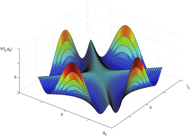
Figure 2: The effective potential in terms of the two scalar fields in the Faddeev-Niemi decomposition

I would like to thank L. Faddeev, E. Langmann and A. Niemi for many valuable discussions on this subject.

References

• [1] Faddeev, L. and Niemi, A.J. Physics Letters B464 (1999) 90
• [2] Faddeev, L. and Niemi, A.J. Nature 387 (1997) 58
• [3] Faddeev, L. and Niemi, A.J. hep-th/0101078
• [4] Coleman, S. and Weinberg, E. Physical Review D, vol.7 no. 6 (1972) 1888
• [5] Abbott, L.F. Acta Phys. Polon. B13 (1982) 33
• [6] Abbott, L.F. Nuclear Physics B185 (1981) 189
• [7] Drummond, I.T. and Fidler, R.W. Nuclear Physics B90 (1975) 77
• [8] Savvidy, G.K. Physics letters B71 (1977) 133
• [9] Nielsen, N.K. and Olesen, P. Nuclear Physics B144 (1978) 376
• [10] Schanbacher, V. Physical Review D, vol.26 no.2 (1982) 489
• [11] Jackiw, R. Physical Review D, vol.9 no. 6 (1974) 1686
• [12] Cho, Y.M., Lee, H. and Pak, D.G. hep-th/0104058
• [13] Cho, Y.M., Lee, H. and Pak, D.G. hep-th/0105198
• [14] Schwinger, J. Physical Review, vol. 82 no.5 (1950) 664
• [15] Brown, L.S. and Weisberger, W.I. Nuclear Physics B157 (1979) 285
• [16] Peskin, M. and Schroeder, D., An introduction to quantum field theory. Addison-Wesley, 1995