We consider some applications of the Renormalization Group flow equations obtained by resorting to a specific class of proper time regulators. Within this class a particular limit that corresponds to a sharpening of the effective width of the regulator is investigated and a procedure to analytically implement this limit on the flow equations is shown. We focus on the critical exponents determination for the $O(N)$ symmetric scalar theory in three dimensions. The large $N$ limit and some perturbative features in four dimensions are also analysed. In all problems examined the results are optimized when the mentioned limit of the proper time regulator is taken.

Pacs 11.10.Hi , 11.10.Kk

1 Introduction

In the past years there has been growing interest for the Renormalization Group (RG) techniques originally inspired to the Kadanoff-Wilson blocking procedure [1], as they represent promising means to investigate areas that are out of reach of the standard perturbative quantum field theory. The central idea is the description of the RG flow in terms of differential equations in the momentum space. Some of the original works on this subject are [2, 3, 4, 5]. More recently, a new formulation of the problem, usually called Exact Renormalization Group (ERG), has been developed [6, 7, 8] (for recent reviews on the subject and on various applications see[9, 10]). The ERG equations are functional differential equations which describe the momentum scale $k$ dependence of a particular functional, usually indicated as average action. This functional is in some sense similar to the effective action, which is the Euclidean generator of the one particle irreducible correlation functions, with the difference that in the former only fluctuations with momenta larger than $k$ are included. This separation between high and low frequencies is realized by the introduction of a smooth cutoff regulator $R_{k}$. A relevant property of this functional is that it interpolates between the classical Euclidean action and the full effective action of the theory, when the scale $k$ is lowered from the ultraviolet cutoff, where the theory is defined by the local classical action, down to zero where all the fluctuations are integrated.

A slightly different approach to the RG flow has been formulated in [11, 12, 13] where an operator cutoff is introduced by means of the Schwinger proper time regulator. The most remarkable feature of this regulator is that it is formulated in a gauge invariant way and it has been already employed to compute the one loop beta function of Yang-Mills theories[14]. Therefore it is a promising tool for any analysis involving gauge theories. Besides that, it has been used to derive flow equations for scalars coupled to fermions[15] and for $O(N)$ scalar theories[16]. The differential equation that describes the flow of the scale dependent action $\Gamma_{k}$ obtained via the proper time regulator is

$$k\;{\partial\Gamma_{k}\over\partial k}=-{1\over 2}{\rm Tr}\;\int_{0}^{\infty}\;{ds\over s}\;k{\partial f_{k}\over\partial k}\;{\rm exp}\;\Big{(}-s{\delta^{2}\Gamma_{k}\over\delta\phi\delta\phi}\Big{)}$$ (1)

with the constraints on the dimensionless cutoff function $f_{k}(x)$ that $f_{k}(0)=1$ and $f_{k}(x\to\infty)=0$ and the initial condition that at some ultraviolet scale $\Lambda$ $\Gamma_{k}$ is equal to the classical action $S$. The trace sums over all the discrete and continuous indices of the field $\phi$. A connection to the perturbative one loop effective action

$$\Gamma^{1-loop}=-{1\over 2}{\rm Tr}\;\int_{0}^{\infty}\;{ds\over s}\;{\rm exp}\;\Big{(}{-s{\delta^{2}S\over\delta\phi\delta\phi}}\Big{)}$$ (2)

is obtained if one neglects the effects of the running by freezing $\Gamma_{k}$ in the r.h.s. of Eq. (1) at its initial condition $S$. In this case $\Gamma_{k}$, due to the condition $f_{k}(0)=1$, coincides at $k=0$ with $\Gamma^{1-loop}$. The running quantity $\Gamma_{k}$ in Eq. (1) corresponds to an infinite resummation of diagrams and therefore improves on the one loop approximation. In practice the regulator $k\partial_{k}f_{k}$ acts as a particular smooth cutoff or weight function in the integration of the modes, selecting only the modes within a small shell centered around the scale $k$.

However there is no direct connection to the smooth cutoff $R_{k}$, introduced in the ERG formalism (see for instance [9]). As a consequence, the proof that in the limit $k\to 0$ the ERG flow of the average action $\Gamma_{k}$ converges to the usual effective action cannot be simply translated to the flow determined by the proper time regulator and a definite indication that this flow actually converges to the full effective action is missing.

It should not be forgotten, however, that for practical purposes it is impossible to deal with the flow of the full action and, typically, a semi-local derivative expansion of the action is introduced to reduce the problem of the evaluation of the flow to a treatable set of coupled partial differential equations. The best approximation analysed so far is the next to leading order in the derivative expansion which corresponds to take the following ansatz for $\Gamma_{k}$

$$\Gamma_{k}[\phi]=\int d^{D}x\Big{(}V(\phi)+{{Z(\phi)}\over{2}}\partial_{\mu}\phi\partial^{\mu}\phi\Big{)}$$ (3)

neglecting all the higher derivative terms, and determine the corresponding differential flow equation for the potential $V$ and for the wave function renormalization $Z$ (obviously $V$ and $Z$ depend on the scale $k$ but this dependence is not explicitly indicated to simplify the notation). Due to this approximation, some uncertainty is introduced about the $k\to 0$ limit of the truncated $\Gamma_{k}$ and a scheme dependence, basically related to the specific regulator employed, appears in the determination of the various physical quantities. This unphysical feature, which would disappear if one could deal with the flow of the full action, cannot be easily quantified. According to this remark, it is worthwhile to compare the predictions obtained with the proper time regulator (although lacking of a convergence proof) with the results obtained from the ERG. In [17] it was noticed that the following choice of the function $f_{k}$

$$f_{k}(sZk^{2})=e^{-sZk^{2}}\sum^{m}_{i=0}{{(sZk^{2})^{i}}\over{i!}},$$ (4)

parametrized in terms of the integer $m$, when the value of $m$ is sufficiently large provides a determination of the critical exponents $\eta,\nu,\omega$ for the one-field scalar theory in $D=3$ dimensions that is certainly comparable to the other determinations obtained in the ERG framework.

In this paper we shall follow this point of view and explore the possibility of explicitly studying the limit in which $m$ is infinite. It will be shown that for a simple particular parametrization it is possible to take the limit $m\to\infty$ and get two coupled equations for the potential and the wave function renormalization which do not contain the parameter $m$ anymore. As noticed in [17] for growing $m$ the proper time regulator selects smaller and smaller momentum shells, centered around the scale $k$, which provide a relevant contribution to the flow differential equations. In this sense the limit $m\to\infty$ corresponds to a procedure of reducing the characteristic width of a smooth cutoff and taking the sharp cutoff limit. Due to the singular nature of this limit, the operation is not unique and depends on the specific smooth cutoff chosen. The central result of this paper is that the equations obtained when $m\to\infty$ yield a determination of the critical exponents which actually agrees very well with the extrapolation of the corresponding values obtained at finite $m$, thus confirming that these universal quantities for large $m$ do not trivially diverge or vanish but rather have a finite sensible limit. Moreover these values are very well compatible with other determinations stemming from different, well established techniques (see [18] or [19]). In Sect. 2 we consider the coupled flow equations of $V$ and $Z$ for a scalar theory obtained with the proper time regulator and determine their form in the limit $m\to\infty$. As a simple application we show that the perturbative two loop anomalous dimension of the scalar field is easily recovered. In Sect. 3 we collect the numerical results on the critical exponents at the non-trivial fixed point in $D=3$ dimensions for finite values of the parameter $m$ and in the limit $m\to\infty$. In Sect. 4 the particular case of the large $N$ limit of the potential equation for a scalar $O(N)$ symmetric theory is considered in order to check that the proper time regulator reproduces the known exact results. The conclusions are summarized in Sect. 5.

2 One component scalar theory

Starting from the evolution equation (1), with the ansatz (3) for the action of a single scalar field theory in $D$ dimensions one can extract the flow equations for $V$ and $Z$. The procedure is outlined in [17] and the result is

$$k{{\partial V}\over{\partial k}}=\alpha k^{D}\Biggl{(}{{Zk^{2}}\over{Zk^{2}+V^{\prime\prime}}}\Biggr{)}^{m+1-D/2}$$ (5)

$$k{{\partial Z}\over{\partial k}}=\alpha k^{D}\Biggl{(}{{Zk^{2}}\over{Zk^{2}+V^{\prime\prime}}}\Biggr{)}^{m+1-D/2}\Biggl{[}{{(m+1-D/2)}\over{Zk^{2}+V^{\prime\prime}}}\biggl{(}-Z^{\prime\prime}$$

$$+{{(4+18D-D^{2})(Z^{\prime})^{2}}\over{24Z}}\biggr{)}+{{(10-D)(m+1-D/2)(m+2-D/2)}\over{6(Zk^{2}+V^{\prime\prime})^{2}}}Z^{\prime}V^{\prime\prime\prime}$$

$$-{{(m+1-D/2)(m+2-D/2)(m+3-D/2)}\over{6(Zk^{2}+V^{\prime\prime})^{3}}}Z(V^{\prime\prime\prime})^{2}\Biggr{]}$$ (6)

where each prime indicates a derivative w.r.t. the field $\phi$ and the constant $\alpha$ is expressed in terms of gamma functions $\Gamma(x)$

$$\alpha={{\Gamma(m+1-D/2)}\over{(4\pi)^{D/2}\Gamma(m+1)}}$$ (7)

One can immediately realize that the quantity $V^{\prime\prime}/(Zk^{2})$ plays a fundamental role when the large $m$ limit of Eqs.(5,2) is considered. In fact if $V^{\prime\prime}/(Zk^{2})>0$ the term raised to the $m$-th power in (5,2) vanishes, and if $V^{\prime\prime}/(Zk^{2})<0$ it diverges (we are not interested here in the broken phase sector and $V^{\prime\prime}/(Zk^{2})<-1$ is never considered). This however does not imply that the universal properties related to Eqs.(5,2) must have a singular (or trivial) behavior for large $m$. Actually in [17] it is found that already for values of $m$ around $10$, the critical exponents are almost $m$-independent.

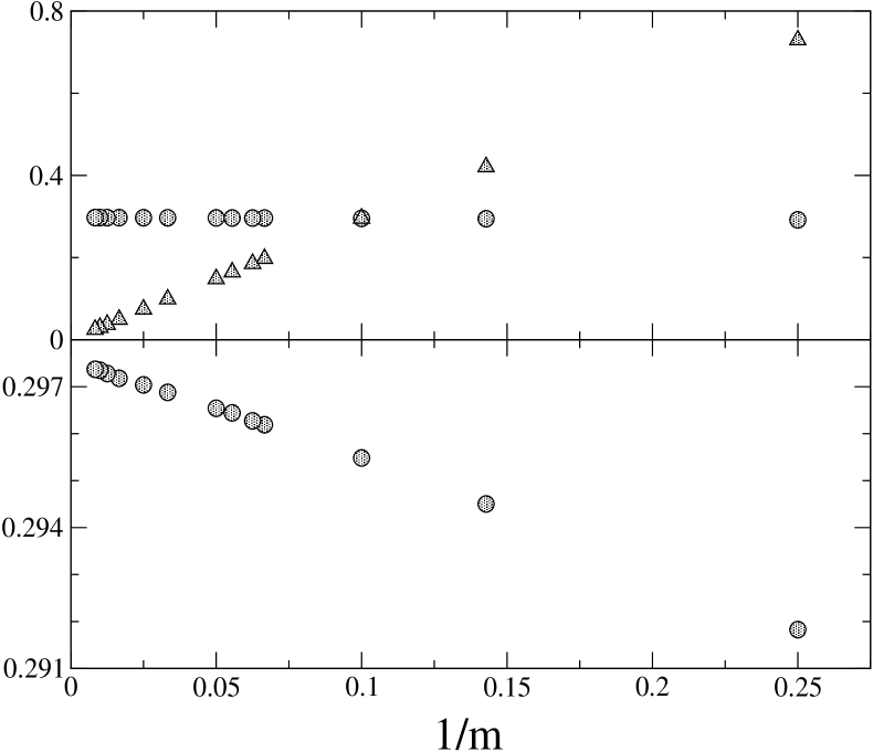
Figure 1: Upper frame: $-10~{}{f^{*}}^{\prime}(0)$ (triangles) and $-10~{}m{f^{*}}^{\prime}(0)$ (circles) at various values of $1/m$, for $N=1$ and to the leading order in the derivative expansion. Lower frame: The same circles of the upper frame, plotted with a magnified scale in the vertical axis.

An interesting information about $V^{\prime\prime}$ can be read in Fig.1 where the particular case of the non-Gaussian fixed point in $D=3$ for the potential only (and $Z=1$ fixed) is examined (more details about this calculation are given in Sect. 3). The triangles in the upper frame of the figure correspond to the values of $-V^{\prime\prime}(\phi=0)$ at the fixed point, properly expressed as a dimensionless variable (see Sect. 3), plotted for some values of $1/m$ (note that in this particular case the curvature at the origin is negative). We consider $1/m$ instead of $m$ because we are essentially interested in the large $m$ limit. The circles in the upper frame correspond to the product $-mV^{\prime\prime}(\phi=0)$. In the lower frame the circles are the same of the upper part of the figure, but plotted on a magnified scale. It is evident from Fig. 1 that $V^{\prime\prime}(\phi=0)$ at the fixed point behaves, at least in first approximation, like $1/m$ for large $m$. Of course this does not simply mean that $mV^{\prime\prime}(\phi=0)$ is a constant. Rather, the plot in the lower frame suggests a behavior like $-mV^{\prime\prime}(\phi=0)=a-b/m$ with $a,b$ positive constants (up to the accuracy considered). However, our aim here is just to find out the leading behavior of $V^{\prime\prime}(\phi=0)$ for large $m$, which, as noticed above, is $1/m$. Supposing that $V^{\prime\prime}$ has the trend of Fig.1, not only at $\phi=0$ but at any value of $\phi$, it would be helpful to redefine the variables in Eqs.(5,2) in such a way that this dependence on $m$ could be compensated.

As a first step we can get rid of the constant $\alpha$ in Eqs. (5,2) by simply redefining $V\to\alpha V$, $\phi\to\sqrt{\alpha}\phi$ and leaving $Z$ unchanged. According to Eq.(3), this operation amounts to rescale the action by the constant $\alpha$. Then, following the indications of Fig.1, we can make a second transformation by replacing $\phi\to\sqrt{m}\phi$. This time the action is not uniformly modified. With the help of the latter substitution we can explicitly take the $m\to\infty$ limit of Eqs. (5,2) and get

$$k{{\partial V}\over{\partial k}}=k^{D}e^{-V^{\prime\prime}/(Zk^{2})}$$ (8)

$$k{{\partial Z}\over{\partial k}}=k^{D}e^{-V^{\prime\prime}/(Zk^{2})}$$

$$\times\Biggl{(}-{{Z^{\prime\prime}}\over{Zk^{2}}}+{{(4+18D-D^{2})(Z^{\prime})^{2}}\over{24Z^{2}k^{2}}}+{{(10-D)Z^{\prime}V^{\prime\prime\prime}}\over{6(Zk^{2})^{2}}}-{{Z(V^{\prime\prime\prime})^{2}}\over{6(Zk^{2})^{3}}}\Biggr{)}$$ (9)

We see that the terms raised to the $m$-th power in (5,2) do not turn into singularities, but instead into exponential terms. In addition, other terms of Eq. (2) do not appear in Eq.(2) because they are suppressed for $m\to\infty$. Eqs. (8,2) can now be used to study the critical properties.

A simple check on Eqs. (5,2) and (8,2) can be performed by looking at the perturbative determination in $D=4$ of the anomalous dimension $\eta$ of the field $\phi$, defined as $\eta=-k\partial_{k}{\rm ln}(\overline{Z})$ where $\overline{Z}$ is the residue of the mass pole of the two point Green function of the theory. The specific truncation of the derivative expansion of the action above considered is actually sufficient to derive the lowest order non-vanishing perturbative contribution to $\eta$ (see for instance [20] where the same calculation, in a different framework, namely starting from the Wegner-Houghton flow equation, has already been performed). In fact if one starts with the classical Euclidean action (we require the invariance under the transformation $\phi\to-\phi$)

$$S={1\over 2}(\partial\phi)^{2}+{{\lambda\phi^{4}}\over{4!}}$$ (10)

then the lowest order values, in the perturbative parameter $\lambda$, of $Z$ and $V$ in (5,2), are respectively $1$ and $\lambda\phi^{4}/4!$. If these lowest order values are inserted in Eq. (2) and the function $Z$ is conveniently expanded in even powers of the field

$$Z=z_{0}+{{z_{2}\phi^{2}}\over 2}+{{z_{4}\phi^{4}}\over{4!}}+...$$ (11)

then, by comparing the terms proportional to $\phi^{2}$ in (2), one immediately sees that $z_{2}$ is $O(\lambda^{2})$. More precisely, by integrating the differential equation from the ultraviolet cutoff $\Lambda$ to the scale $k<<\Lambda$ (but still $k$ much larger than any other infrared scale such as the field mass pole)

$$z_{2}={{(m+1)}\over{16\pi^{2}}}{{\lambda^{2}}\over{6k^{2}}}+O(\lambda^{3})+O(1/\Lambda^{2})$$ (12)

Consequently, $z_{0}$, which at the leading order is $z_{0}=1$ (as it follows from (10) and (11)), to the next to leading order gets a $O(\lambda^{2})$ contribution from $z_{2}$ that enters the flow equation of $z_{0}$ through the term $Z^{\prime\prime}$ in Eq. (2). We get

$$k{{\partial z_{0}}\over{k}}=-{{(m+1)}\over{6m}}\left({{\lambda}\over{16\pi^{2}}}\right)^{2}+O(\lambda^{3})$$ (13)

The two point Green function is obtained from the double functional derivative of (3) at $\phi=0$. It is easy to realize that to the next to leading order in the derivative expansion we get $\Gamma^{(2)}(p^{2})=z_{0}p^{2}+V^{\prime\prime}(\Phi=0)$ and therefore, to this order, $\overline{Z}=z_{0}$. It follows

$$\eta={{(m+1)}\over{6m}}\left({{\lambda}\over{16\pi^{2}}}\right)^{2}+O(\lambda^{3})$$ (14)

The important result here is that the perturbative value of $\eta$ (see e.g. [18]) corresponds to the large $m$ limit of Eq. (14), which is in agreement with our conjecture that the physically relevant results are obtained for $m\to\infty$.

One remark is to be made here about other terms neglected in the derivative expansion (3) that are $O(\lambda^{2})$. In fact terms like $Y\phi^{2}\partial^{n}\phi\partial^{n}\phi$ with $n\geq 2$, which are neglected to order $O(\partial^{2})$, can be computed with the same method employed to determine Eqs.(5,2)and it turns out that $Y\propto\lambda^{2}/k^{2n}$. However the contribution of $Y$ to $\Gamma^{(2)}(p^{2})$ is proportional to $\lambda^{2}(p^{2}/k^{2})^{n}$ and, as long as we are interested in a momentum range where $k^{2}$ is much larger than a mass pole, then $k^{2}>>p^{2}$ and, consistently, we can neglect the contributions of $Y$ and similar terms which are suppressed by the factor $(p^{2}/k^{2})^{n}$.

Finally we turn to Eqs. (8,2) and perform the same perturbative analysis. In order to get the same normalization used to derive Eq. (14), one has to remember that, globally, the following substitutions have been performed to go from (5,2) to (8,2): $V\to\alpha V$, $\phi\to\sqrt{\alpha m}\phi$ and no rescaling on $Z$. As a consequence, instead of starting with the classical action $S$ in (10) we have to start with a modified action $\widehat{S}$, equal in form to (10), but with $\lambda$ replaced with $\widehat{\lambda}=\alpha m^{2}\lambda$, which for $m\to\infty$ becomes (see Eq. (7))

$$\widehat{\lambda}={\lambda\over{16\pi^{2}}}$$ (15)

Note that since $Z$ is unchanged the initial value in (10), $Z=1$, i.e. $z_{0}=1$, is unchanged too. A non-vanishing initial value for $z_{2}$ would have required a rescaling according to the definition (11). After this remark, it is straightforward to derive $z_{2}$ and $\eta$ (through $z_{0}$) from Eq. (2):

$$z_{2}={{\widehat{\lambda}^{2}}\over{6k^{2}}}+O(\widehat{\lambda}^{3})+O(1/\Lambda^{2})$$ (16)

$$\eta={{\widehat{\lambda}^{2}}\over{6}}+O(\widehat{\lambda}^{3})$$ (17)

As expected the large $m$ limit of Eq. (14) coincides with Eq. (17) which is the perturbative value of $\eta$.

3 Numerical results

In this Section we focus on the problem of determining, through a numerical analysis, the fixed point solutions of our flow equations and the critical exponents $\nu$ and $\omega$ related to the eigenvalues of the linearized version of the flow equation around the fixed point. In particular we are interested in the three dimensional case for which a large number of determinations of these universal quantities, obtained employing many different techniques, is available in the literature (see e.g. [18, 19, 9]). Therefore, for the rest of this Section we set $D=3$.

The numerical determination of the exponents for this particular kind of proper time regulated flow, was started in [17]. There, $\nu$, $\omega$ and the anomalous dimension $\eta$ of the one component scalar theory, determined by the numerical resolution of Eqs. (5) and (2) are displayed for increasing values of the parameter $m$ and the data show a monotonous dependence on $m$. In particular $\nu$ and $\omega$ are determined up to $m=9$ and $\eta$ up to $m=40$. Since in the second case $m$ is sufficiently large, the asymptotic value (for $m\to\infty$) of $\eta$ is obtained through a numerical fit in [17] and it is only claimed that $\nu$ and $\omega$ converge to finite values.

In the following we refine this analysis and evaluate $\eta$, $\nu$ and $\omega$ to the leading order ($O(\partial^{0})$) in the derivative expansion (by solving the potential part of the flow keeping $Z=1$ and $\eta=0$ fixed), and to the next to leading order ($O(\partial^{2})$) (by solving the full coupled problem for the potential and the wave function renormalization). In most cases we push the parameter $m$ up to $m=120$, which clearly shows the numerical trend of the exponents and then we compare the obtained values with the ones determined from the equations (8) and (2) which hold for $m\to\infty$. We also extend the analysis to the $O(N)$ symmetric theory limiting ourselves to the $O(\partial^{0})$ approximation in the derivative expansion and derive $\nu$ and $\omega$ for $N=2,3,4$, for increasing values of $m$ and for $m\to\infty$.

In order to perform the numerical analysis of the flow equations to find the fixed point solution and the related critical exponents we need to reformulate Eqs. (5) and (2) in terms of dimensionless variables. At the same time, to simplify the numerical procedure, it is convenient to get rid of the constant $\alpha$ through the transformation already used in the previous Section and, more important, to replace the differential equation for the potential with the corresponding equation for the potential derivative w.r.t. the field. In fact, as already noticed in [5, 8] the former equation is stiff and therefore more difficult to treat. To this aim we introduce the new dimensionless variables $t={\rm ln}(\Lambda/k)$, $x=k^{-(1+\eta)/2}\phi/\sqrt{\alpha}$, $V_{d}(t,x)=k^{-3}V(k,\phi)/\alpha$ and $Z_{d}(t,x)=k^{\eta}Z(k,\phi)$ where the subscript $d$ has been used to indicate the dimensionless potential and wave function renormalization, $\alpha$ is defined in Eq.(7) and, as before, $\eta$ indicates the anomalous dimension of the field. Finally we define the potential derivative $f(x,t)=\partial_{x}V_{d}(t,x)$. In terms of these new variables Eqs.(5,2) read

$$\partial_{t}f={{(5-\eta)}\over{2}}f-{{(1+\eta)}\over{2}}xf^{\prime}-\left(m-{1\over 2}\right)\Biggl{(}{{Z_{d}}\over{Z_{d}+f^{\prime}}}\Biggr{)}^{m-3/2}{{({Z_{d}}^{\prime}f^{\prime}-Z_{d}f^{\prime\prime})}\over{(Z_{d}+f^{\prime})^{2}}}$$ (18)

$$\partial_{t}Z_{d} = -\eta Z_{d}-{{(1+\eta)}\over{2}}x{Z_{d}}^{\prime}+\Biggl{(}{{Z_{d}}\over{Z_{d}+f^{\prime}}}\Biggr{)}^{m-1/2}\Biggl{[}{{(m-1/2)}\over{Z_{d}+f^{\prime}}}\biggl{(}{Z_{d}}^{\prime\prime}-{{49({Z_{d}}^{\prime})^{2}}\over{24Z_{d}}}\biggr{)}$$ (19)

$$-{{7(m^{2}-1/4)}\over{6(Z_{d}+f^{\prime})^{2}}}{Z_{d}}^{\prime}f^{\prime\prime}+{{(m^{2}-1/4)(m+3/2)}\over{6(Z_{d}+f^{\prime})^{3}}}Z_{d}(f^{\prime\prime})^{2}\Biggr{]}$$

Analogously, we can rewrite Eqs. (8) and (2) in the dimensionless form

$$\partial_{t}f={{(5-\eta)}\over{2}}f-{{(1+\eta)}\over{2}}xf^{\prime}+e^{-f^{\prime}/Z_{d}}\left({{f^{\prime\prime}}\over{Z_{d}}}-{{f^{\prime}{Z_{d}}^{\prime}}\over{Z_{d}^{2}}}\right)$$ (20)

$$\partial_{t}Z_{d}=-\eta Z_{d}-{{(1+\eta)}\over{2}}x{Z_{d}}^{\prime}+e^{-f^{\prime}/Z_{d}}\Biggl{(}{{{Z_{d}}^{\prime\prime}}\over{Z_{d}}}-{{49({Z_{d}}^{\prime})^{2}}\over{24Z_{d}^{2}}}-{{7{Z_{d}}^{\prime}f^{\prime\prime}}\over{6Z_{d}^{2}}}+{{(f^{\prime\prime})^{2}}\over{6Z_{d}^{2}}}\Biggr{)}$$ (21)

The fixed points are the $t$-independent solutions $f^{*}(x)$ and ${Z_{d}}^{*}(x)$ of Eqs. (18,19), or Eqs. (20,21). The resolution of the coupled ordinary differential fixed point equations also provide the value of $\eta$ at the fixed point. In order to find $\nu$ and $\omega$ we need to introduce small $t$-dependent perturbations around the fixed point and reduce the problem to coupled linear equations in the perturbations. The perturbations are parametrized in the following way

$${V_{d}}(t,x)={V_{d}}^{*}(x)+e^{\lambda t}{\rm v}(x)$$

$$Z_{d}(t,x)={Z_{d}}^{*}(x)+e^{\lambda t}z(x)$$ (22)

The corresponding relation for the potential derivative $f(t,x)$ is obtained by deriving the first line and, by indicating with $h(x)$ the derivative of ${\rm v}(x)$, one has

$$f(t,x)=f^{*}(x)+e^{\lambda t}h(x)$$ (23)

The resolution of the linear equations provides the eigenvalues $\lambda$ and the eigenvectors ${\rm v}(x)$, $h(x)$ and $z(x)$ which govern the flow close to the fixed point. In particular for the problem considered we expect, besides the Gaussian fixed point, which corresponds to $f^{*}(x)=\eta=0,~{}{Z_{d}}^{*}(x)=const$, only the Wilson-Fisher fixed point, which has just one relevant eigenvector ($\lambda$ positive). The exponent $\nu$ is defined as the inverse of the only positive eigenvalue and $\omega$ is the opposite of the less negative eigenvalue.

We shall also consider the $O(N)$ theory but only in the lowest order approximation $O(\partial^{0})$, and in this case the dimensionless form of the flow equation for the derivative of the potential is

$$\partial_{t}f={5\over 2}f-{1\over 2}xf^{\prime}+\left(m-{1\over 2}\right)\Biggl{[}\left({1\over{1+f^{\prime}}}\right)^{m+1/2}f^{\prime\prime}$$

$$+(N-1)\left({1\over{1+f/x}}\right)^{m+1/2}\left({{f^{\prime}}\over x}-{{f}\over{x^{2}}}\right)\Biggr{]}$$ (24)

where in addition to the longitudinal field contribution, which is equal to the one for the single component field, there are $(N-1)$ contributions of the transverse fields. Finally the limit $m\to\infty$ of Eq. (3) becomes

$$\partial_{t}f={5\over 2}f-{1\over 2}xf^{\prime}+e^{-f^{\prime}}f^{\prime\prime}+(N-1)e^{-f/x}\left({{f^{\prime}}\over x}-{{f}\over{x^{2}}}\right)$$ (25)

It must be noted that Eq. (3) at $m=1$ and for any $N$ is exactly equal to the flow equations derived in the $O(\partial^{0})$ approximation in [8, 21] and therefore a good check on our numerical outputs, at least for $m=1$, is to compare them to the results reported in [21].

The numerical resolution of the equations is thoroughly explained in [8] and here we just shortly summarize the procedure and skip the details. The two coupled ordinary differential equations that determine the fixed point have some boundary conditions defined at $x=0$ and the rest at large $x$. In fact, by requiring the symmetry of the theory under the transformation $x\to-x$, one gets the following conditions: ${Z^{*}_{d}}^{\prime}(0)=f^{*}(0)=0$. In addition, the normalization ${Z^{*}_{d}}(0)=1$ is imposed. (As noticed in [17] the flow equations here considered are reparametrization [8, 22] invariant, and, as a consequence the universal quantities are independent of the particular normalization chosen, and this has been checked explicitly in the numerical analysis of [17]). On the other hand, the equations themselves constrain the asymptotic behavior of the solution at large $x$, up to two constant factors, one for each of the two functions $Z_{d}^{*}(x)$ and $f^{*}(x)$. The eigenvalue problem for the linear equations is totally analogous because the same symmetry must be imposed at $x=0$ and the same kind of constraints can be derived from the equations at large $x$.

These boundary conditions are sufficient to solve the problem (and determine the fixed point and the critical exponents) by means, for instance, of the shooting method[8]. In particular, for our analysis, we have implemented this method by making use of the NAG libraries and this has allowed us to improve on the accuracy of the results of [17] and to test the equations for higher values of $m$.

One result of the numerical analysis has already been presented in Fig. 1, where the curvature at $x=0$ of the non-Gaussian fixed point solution for some values of $m$, is plotted. Namely the triangles in the upper frame of Fig. 1 are the values of $-10~{}{f^{*}}^{\prime}(0)$ determined from Eq. (18), in the $O(\partial^{0})$ approximation i.e. with $Z_{d}=1$ and $\eta=0$, plotted versus $1/m$. The circles in the upper and lower frames correspond instead to the product $-10~{}m{f^{*}}^{\prime}(0)$ displayed with two different scales on the vertical axis. This plot has already been commented in Sect. 2.

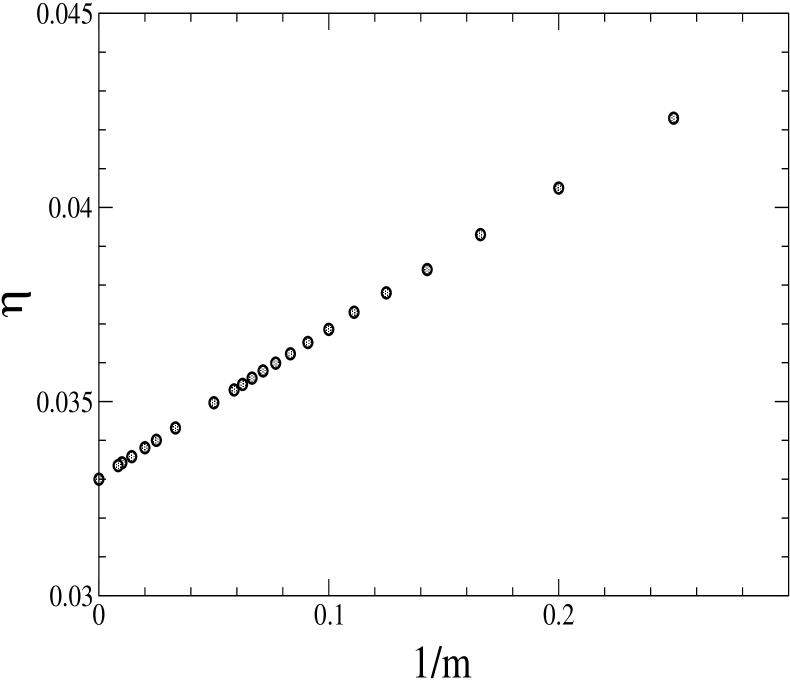
Figure 2: Anomalous dimension $\eta$ at various values of $1/m$, including $1/m=0$, for $N=1$ and to the next to leading order in the derivative expansion.

Fig.2 shows the anomalous dimension $\eta$ at the fixed point for the $N=1$ case, plotted versus $1/m$ up to $m=120$. Note that we have inserted at $1/m=0$ the value of $\eta$ obtained from the fixed point solution of Eqs. (20,21) whereas all the other points come from Eqs. (18,19). Some of these points are already reported in [17], where however the maximum value of $m$ considered was $m=40$. The convergence in Fig.2 of the values obtained at finite $m$ to the one at $1/m=0$ is clear.

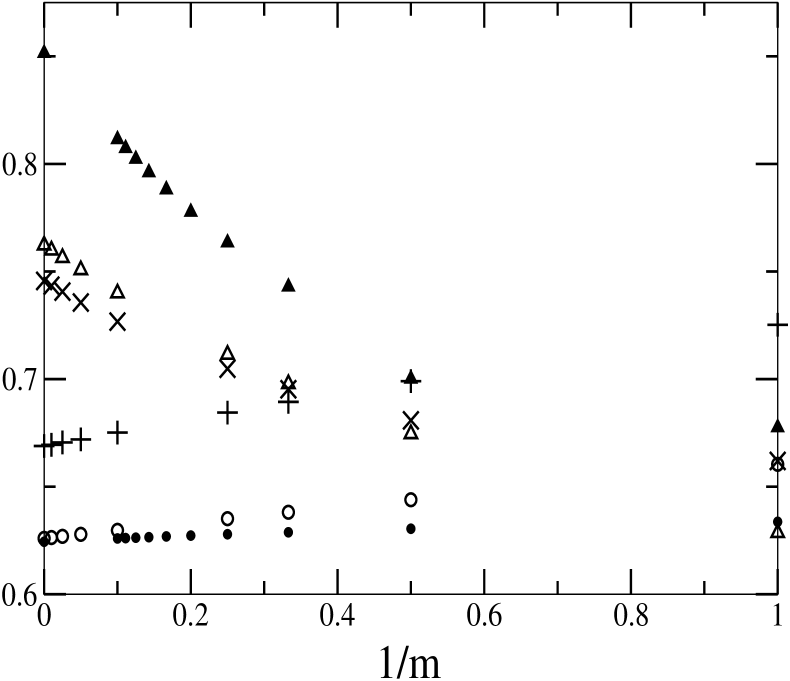
Figure 3: Critical exponents at various values of $1/m$, including $1/m=0$. Empty and full black circles are respectively the $O(\partial^{0})$ and $O(\partial^{2})$ values of $\nu$ for $N=1$. Empty and full black triangles are respectively the $O(\partial^{0})$ and $O(\partial^{2})$ values of $\omega$ for $N=1$. Finally the $+$ and the $\times$ correspond respectively to the $O(\partial^{0})$ value of $\nu$ and to the $O(\partial^{0})$ value of $\omega$ for $N=2$.

In Fig. 3 we have collected the same kind of results for $\nu$ and $\omega$. Namely, for the $N=1$ case, empty and black circles are respectively the $O(\partial^{0})$ and $O(\partial^{2})$ values of $\nu$ and empty and black triangles the same for $\omega$. Again the points on the vertical axis $1/m=0$ are obtained from Eqs.(20,21) and the others from Eqs. (18,19). Note that for the $O(\partial^{0})$ case we evaluated the exponents up to $m=120$ whereas for the $O(\partial^{2})$ we stopped at $m=10$ because we believe that even at this level the trend of the data and their convergence to the $1/m=0$ case is evident.

Two remarks are in order. The first one concerns the fact that, for those values of $m$ for which the comparison is possible, we have found agreement with the numerical data of [17], except for $\omega$ to the $O(\partial^{2})$ order, whose values plotted in Fig. 3 (black triangles) differ from those of [17]. In fact, we have noticed that in this case the results are more sensible to the maximum value of $x$ considered in the numerical integration of the equations and the routines used here allowed a more careful analysis and a more accurate determination of the data. The second remark is about the convergence of the derivative expansion. The $O(\partial^{0})$ and the $O(\partial^{2})$ values of $\nu$ at $1/m=0$ are almost equal, suggesting that the derivative expansion converges very rapidly for this particular exponent. The situation for $\omega$ is rather different, and one can only guess that the higher order determinations of this quantity lie between the $O(\partial^{0})$ and the $O(\partial^{2})$ estimates. Therefore it seems that the rapid convergence concerns only the relevant eigenvalue.

The findings of the numerical analysis for $\nu$ and $\omega$ in the $N=2$ theory and $O(\partial^{0})$ approximation are also reported in Fig. 3. The symbol $+$ is associated to the values of $\nu$ and the $\times$ to $\omega$. In this case we have determined the exponents up to $m=120$ and again the convergence toward the values obtained at $1/m=0$ is clear. On the basis of these results, we do not consider so many values of $m$ for $N=3,4$, and determine $\nu$ and $\omega$ only at $m=1,2$ and at $1/m=0$ (see the Tables below).

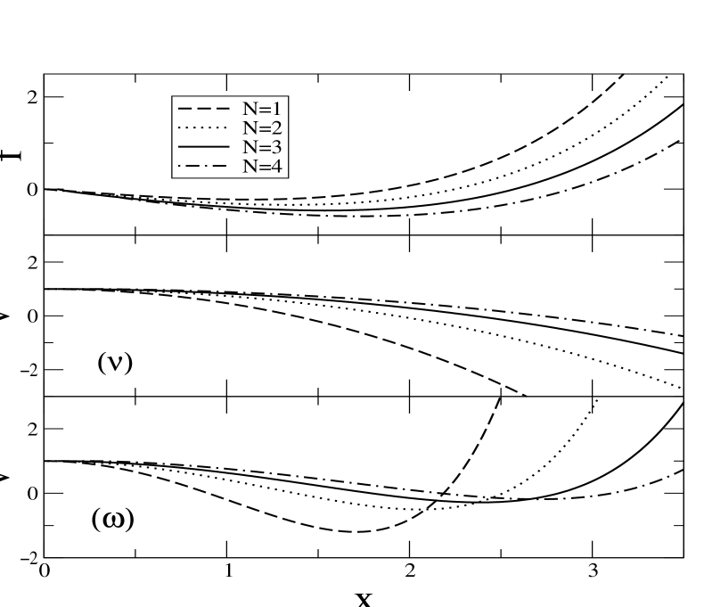
Figure 4: The Wilson-Fisher fixed point derivatives of the potential (upper frame) and the eigenvectors corresponding to the exponent $\nu$ (central frame) and those corresponding to the exponent $\omega$ (lower frame), for $N=1,2,3,4$, all to the $O(\partial^{0})$ order.

In Fig. 4 we report various plots obtained from Eq.(25), which is valid to the $O(\partial^{0})$ order, in the four cases $N=1,2,3,4$. In the upper frame, the fixed point derivative of the potential is shown, in the central frame the eigenvector corresponding to the critical exponent $\nu$ and, in the lower one, the eigenvector corresponding to $\omega$. The trend observed is a flattening of the curves for increasing $N$.

Finally in Table I and II we report the numerical values of the exponents only at $m=1,2,\infty$. Incidentally we note that $\eta$ at $m=\infty$ in Table I is practically the same of the value $\eta=0.0329$ quoted in [17] as the output of a fit to the data collected up to $m=40$. We also note that the $O(\partial^{0})$ results at $m=1$ are totally in agreement with those of [21] which, as discussed above, was expected because in this particular case the flow equations considered here and in [21] coincide.

A comparison with the critical exponents determined by different methods (see [18, 19, 9]) globally indicates a better agreement with the values at $m=\infty$ rather than with those at $m=1$ or $m=2$. This supports the idea that the optimization of the proper time cutoff is achieved in the large $m$ limit, which can be interpreted as a sharp limit of this class of regulators. Conversely, the optimization criterion suggested in [23], obtained by establishing a relation between the proper time regulator and the $R_{k}$ class of regulators introduced in the ERG approach, does not seem to be particularly satisfying. In fact it predicts that the optimum value of our parameter (note the difference in the definition of $m$ here and in [23]) is $m=3/2$ and the exponents at $m=3/2$ are expected to be between those found at $m=1$ and those at $m=2$ in Tables I,II.

4 $O(N)$ theory at $N=\infty$

Another interesting check on the proper time flow equations concerns the problem of the $O(N)$ symmetric theory in the limit $N\to\infty$. In this case the $O(N)$ theory reduces to the spherical model which is exactly solved. At the same time in this limit the flow equation for the potential becomes a close decoupled equation and the main universal features of the spherical model are recovered [2, 24, 21]. Our aim is to check that these properties survive when we interchange the two limit procedures and consider first $m\to\infty$ and then $N\to\infty$. As noticed before, to the lowest order in the derivative expansion, the potential flow equation (3) at $m=1$ is equal to the one considered in [21], where a detailed analysis of the $N=\infty$ case is presented. So at least for $m=1$ the proper time flow of the potential reproduces the results shown in [21] and in particular the presence, besides the Gaussian fixed point, of the Wilson-Fisher fixed point for $D<4$, and the correct determination of the eigenvalue spectrum of the linearized equation in both cases. Then we examine the problem at $m\not=1$.

Let us consider the more general version in $D$ dimensions of Eq.(3), which was obtained in $D=3$. For large $N$, the leading behavior is given by the last term in the r.h.s.. As it has been done for the constant $\alpha$, we can make one more rescaling $f\to Nf$ and $x\to\sqrt{N}~{}x$ which allows to take straightforwardly the limit $N\to\infty$

$$\partial_{t}f=\left({{D+2}\over 2}-{{m}\over{x^{2}(1+f/x)^{m+1}}}\right)f-\left({{D-2}\over 2}-{{m}\over{x^{2}(1+f/x)^{m+1}}}\right)x~{}f^{\prime}$$ (26)

The fixed point structure is obtained by requiring $\partial_{t}f=0$. Actually we are interested in the universal properties at the fixed point and, as shown in [2, 24], to determine the critical exponents it is not necessary to have the explicit fixed point solution $f^{*}(x)$, but it is sufficient to determine the essential singularities of the equation. From the structure of Eq. (26) one realizes that there is a non-zero value of $x$ at which the function $f^{*}$ vanishes. In fact if at $x=\overline{x}$ the second bracket in (26) vanishes, then it must be $f^{*}(\overline{x})=0$ since the first bracket at $x=\overline{x}$ does not vanish. Therefore from the second bracket it follows that $\overline{x}=\sqrt{2m/(D-2)}$. We can now expand around $\overline{x}$. By setting in the fixed point equation $x=\overline{x}+\Delta x$ and $f^{*}(x)=f^{*^{\prime}}(\overline{x})\Delta x+O((\Delta x)^{2})$ we get the value of $f^{*^{\prime}}(\overline{x})$:

$$(m+1)f^{*^{\prime}}(\overline{x})={4\over{D-2}}-2$$ (27)

With this information we can analyse the corresponding linearized equation and, recalling Eq. (23), we get

$$\lambda h=\left({{D+2}\over 2}-{{m}\over{x^{2}(1+f^{*}/x)^{m+1}}}\right)h$$

$$-\left({{D-2}\over 2}-{{m}\over{x^{2}(1+f^{*}/x)^{m+1}}}\right)xh^{\prime}+{{m(m+1)(f^{*}-xf^{*^{\prime}})}\over{x^{3}(1+f^{*}/x)^{m+2}}}h$$ (28)

At $x=\overline{x}$ the coefficient of $xh^{\prime}$ in brackets vanishes and therefore from Eq. (4) it follows that either $h^{\prime}(\overline{x})/h(\overline{x})$ is singular (with a simple pole singularity) or it is finite and in this case the eigenvalue $\lambda$ is uniquely determined (remember that $f^{*}(\overline{x})=0$). If one requires that the eigenvector $h(x)$ has no singularity and admits the power expansion around $\overline{x}$,

$$h(x)=\sum_{i=n}^{\infty}a_{i}(x-\overline{x})^{i}$$ (29)

where the lowest power $n$ is a non-negative integer, then one can study the behavior of Eq.(4) close to $x=\overline{x}$. The quantity $h^{\prime}(x)/h(x)$ is replaced by the leading singular term $n/(x-\overline{x})$ but the pole is canceled by the vanishing coefficient of $h^{\prime}(x)/h(x)$, and therefore with the help Eq. (27), at $x=\overline{x}$ Eq.(4) is reduced to the simple relation among the eigenvalue $\lambda$, the non-negative integer $n$ and the number of dimensions $D$

$$\lambda=D-2-2n$$ (30)

which is the spectrum of the spherical model eigenvalues.

We are also able to derive the eigenvalues relative to the Gaussian fixed point. In fact, going back to the linearized equation (4), by evaluating it at the Gaussian fixed point $f^{*}_{G}(x)=0$, and expanding around $\overline{x}$, one gets the new spectrum

$$\lambda_{G}=2-(D-2)n$$ (31)

At the upper critical dimension $D=4$ the two spectra (30) and (31) coincide. Obviously for the simple case of the Gaussian fixed point one could directly start with the linearized equation of the potential, rather than using the potential derivative $f$. By indicating with ${\rm v}_{G}$ the eigenvector of the potential, the $N=\infty$ flow equation for the potential, linearized around the Gaussian fixed point $V_{G}^{*}=0$, reads

$$(\lambda-D){\rm v}_{G}=\left({m\over x}-{{(D-2)}\over 2}x\right){{\rm v}_{G}}^{\prime}$$ (32)

The above equation is solved explicitly

$${\rm v}_{G}=c\left(x^{2}-{{2m}\over{(D-2)}}\right)^{(D-\lambda)/(D-2)}$$ (33)

where $c$ is the integration constant. If we require polynomial (not constant) solutions of the problem, which preserve the symmetry $x\to-x$, we have $(D-\lambda_{G})/(D-2)=n+1$ where $n$ is again a non-negative integer. Therefore we have found again relation (31). It should be noted that here we have the full solution (33) of Eq. (32) and its parity must be explicitly required. Conversely this constraint must not be applied to the expansion considered above, around the point $\overline{x}\not=0$.

The relevant point of the above analysis is that in both eigenvalue spectra for the Gaussian and the non-trivial fixed point, the dependence on the proper time regulator parameter $m$ has disappeared and the structure of the eigenvalue spectrum is valid for any value of $m$. We expect that by performing first the $m\to\infty$ and then the $N\to\infty$ limit in the flow equation, these universal properties are preserved. To prove this point we perform on Eq. (25) the same rescaling used to derive Eq.(26) and get

$$\partial_{t}f=\left({{D+2}\over 2}\right)f-\left({{D-2}\over 2}\right)x~{}f^{\prime}+e^{-f/x}\left({f^{\prime}\over{x}}-{f\over{x^{2}}}\right)$$ (34)

As before, in the fixed point equation there is a value of the dimensionless field, $\overline{x}=\sqrt{2/(D-2)}$, such that $f^{*}(\overline{x})=0$ and, as can be seen by expanding the fixed point equation around $\overline{x}$, ${f^{*}}^{\prime}(\overline{x})=2(4-D)/(D-2)$. Then we can analyse the linearized version of Eq.(34) around the Gaussian and the non-Gaussian fixed point as we did for Eq.(4) and it is straightforward to derive again the two equations for $\lambda_{G}$ and $\lambda$, (31) and (30), respectively. Therefore, even in this case, the flow equation obtained in the limit $m\to\infty$ retain the relevant universal properties observed at $m=1$.

5 Conclusions

As already discussed in the Introduction, there is no proof of convergence of the proper time RG flow to the full effective action when the infrared scale $k$ is lowered to zero, so that all modes in the momentum space are effectively taken into account. On the other hand we have collected here some evidences showing the reliability of the predictions of this flow equations which are certainly comparable to those of the ERG.

The proper time regulator is parametrized by a number $m$, which is restricted to integer values. According to [17], $m$ is related to the effective width associated to the proper time cutoff and larger values of $m$ correspond to more narrow widths. We have shown that for a particular redefinition of the quantities entering the flow equations, it is possible to formally take the limit $m\to\infty$ and get new differential equations which are totally $m$ independent.

Then, in some numerical examples, we checked that the values of the critical exponents $\eta$, $\nu$ and $\omega$ as functions of the parameter $m$ are effectively converging to the numerical values obtained from the asymptotic (in the sense of $m\to\infty$) equations. As a consequence of this analysis we get an optimized determination of the above exponents for $m\to\infty$ which are certainly in very good agreement with the numbers coming from different methods. Other aspects investigated are the perturbative determination of the anomalous dimension in $D=4$ and the comparison with the spherical model in the large $N$ limit. In both cases the asymptotic equations produce results that totally agree with the ones coming from the $m$ dependent flow equations at large $m$. In the $N=\infty$ case, actually, the universal quantities show no dependence at all on $m$.

TABLE I

$N=1$
	$\eta$	$\nu$		$\omega$
$m$	$O(\partial^{2})$	$O(\partial^{0})$	$O(\partial^{2})$	$O(\partial^{0})$	$O(\partial^{2})$
$1$	0.0653	$0.6604$	$0.6337$	$0.629$	$0.677$
$2$	0.0507	$0.6439$	$0.6304$	$0.674$	$0.700$
$\infty$	0.0330	$0.6260$	$0.6244$	$0.762$	$0.851$

Table 1: Critical exponents for $N=1$ at the Wilson-Fisher fixed point to the leading, $O(\partial^{0})$, and next to leading order, $O(\partial^{2})$, in the derivative expansion.

TABLE II

	$N=2$		$N=3$		$N=4$
$m$	$\nu$	$\omega$	$\nu$	$\omega$	$\nu$	$\omega$
$1$	$0.7252$	$0.662$	$0.7809$	$0.707$	$0.8238$	$0.751$
$2$	$0.6990$	$0.681$	$0.7498$	$0.700$	$0.7924$	$0.726$
$\infty$	$0.6689$	$0.746$	$0.7102$	$0.734$	$0.7481$	$0.729$

Table 2: Critical exponents $\nu$ and $\omega$ for $N=2,3,4$ at the Wilson-Fisher fixed point to the leading order $O(\partial^{0})$ in the derivative expansion.

References

- [1] L.P. Kadanoff, Physica 2, 263, (1966); K.G. Wilson, Phys. Rev. B4, 3174 and 3184, (1971); K.G. Wilson and M.E. Fisher, Phys. Rev. Lett. 28, 240, (1972); K.G. Wilson and J. Kogut, Phys. Rep. 12, 75, (1974).
- [2] F. J. Wegner and A. Houghton, Phys. Rev A8, 401 (1973).
- [3] J.F. Nicoll, T.S. Chang and H.E. Stanley, Phys. Rev. Lett. 33, 540 (1974); Phys. Rev. A 13, 1251 , (1976); J.F. Nicoll and T.S. Chang, Phys. Lett. A62, 287, (1977); T.S. Chang, D. D. Vvedensky and J.F. Nicoll, Phys. Rep. 217, 280, (1992).
- [4] J. Polchinski, Nucl. Phys. B 231, 269 (1984).
- [5] A. Hasenfratz and P. Hasenfratz, Nucl Phys. B270, 685 (1986).
- [6] C. Wetterich, Nucl. Phys. B352, 529, (1991); Z. Phys. C57, 451, (1993); C60 461, (1993); Phys Lett. B301, 90, (1993).
- [7] T. Morris, Int. J. Mod. Phys. A 9 2411, (1994).
- [8] T. Morris, Phys. Lett. B329, 241, (1994).
- [9] J. Berges, N. Tetradis and C. Wetterich, Nonperturbative renormalization group flow in quantum field theory and statistical physics, Preprint: MIT-CTP-2980, HD-THEP-00-26, May 2000 and hep-ph/0005122. Submitted to Phys.Rep.
- [10] C. Bagnuls and C. Bervillier, Exact renormalization group equations. An introductory review, Preprint: SACLAY-SPHT-T00-008, SACLAY-SPHT-S00-009, Feb 2000 and hep-th/0002034. Submitted to Phys.Rep.
- [11] M. Oleszczuk, Z. Phys. C64, 533, (1994).
- [12] R. Floreanini and R. Percacci, Phys. Lett. B356, 205, (1995).
- [13] S.-B. Liao, Phys. Rev. D53, 2020, (1996).
- [14] S.-B. Liao, Phys. Rev. D56, 5008, (1997).
- [15] B.J. Schaefer and H.J. Pirner, Nucl. Phys. A627, 481, (1997); Nucl. Phys. A660 439, (1999); J. Meyer, G. Papp, H.J. Pirner and T. Kunihiro, Phys. Rev. C61, 035202, (2000); G. Papp, B.J. Schaefer, H.J. Pirner and J. Wambach, Phys. Rev. D61, 096002, (2000).
- [16] O. Bohr, B.J. Schaefer and J. Wambach, Renormalization group flow equations and the phase transition in models, Preprint July 2000. e-Print Archive: hep-ph/0007098.
- [17] A. Bonanno and D. Zappalà, Phys. Lett. B504, 181, (2001).
- [18] J. Zinn-Justin, “Quantum Field Theory and Critical Phenomena” Oxford Science Publications, (1990), Clarendon Press Oxford.
- [19] R. Guida and J. Zinn-Justin, Nucl. Phys. B 489 [FS], 626, (1997); J. Phys. A 31, 8103, (1998).
- [20] A. Bonanno and D. Zappalà, Phys. Rev. D57, 7383 (1998); A. Bonanno, V. Branchina, H. Mohrbach and D. Zappalà, Phys. Rev. D60, 065009, (1999).
- [21] T.R. Morris and M.D. Turner, Nucl. Phys. B 509 [FS], 637, (1998).
- [22] J. Comellas, Nucl. Phys. B 509, 662, (1998).
- [23] D.F. Litim, Phys.Lett. B486, 92, (2000); D.F. Litim, Optimized Renormalization Group Flows, CERN-TH-2001-084, Mar 2001, e-Print Archive: hep-th/0103195.
- [24] J. Comellas and A. Travesset, Nucl. Phys. B 498, 539, (1997).