Twisted Vortices in a Gauge Field Theory

We inspect a particular gauge field theory model that describes the properties of a variety of physical systems, including a charge neutral two-component plasma, a Gross-Pitaevskii functional of two charged Cooper pair condensates, and a limiting case of the bosonic sector in the Salam-Weinberg model. It has been argued that this field theory model also admits stable knot-like solitons. Here we produce numerical evidence in support for the existence of these solitons, by considering stable axis-symmetric solutions that can be thought of as straight twisted vortex lines clamped at the two ends. We compute the energy of these solutions as a function of the amount of twist per unit length. The result can be described in terms of a energy spectral function. We find that this spectral function acquires a minimum which corresponds to a nontrivial twist per unit length, strongly suggesting that the model indeed supports stable toroidal solitons.

Recently, a gauge field theory model with two charged bosons has been conceived, to describe a two-component plasma of negatively and positively charged particles [1]. But this model also appears to describe a large variety of other physical phenomena, including a Gross-Pitaevskii functional of two band superconductivity [2] and the bosonic sector in the Salam-Weinberg model in the limit where the Weinberg angle $\theta_{W}=0$ [3]. In [1] (see also [3]) it has been proposed that the model supports stable, self-confining and knot-like solitonic configurations. This would be somewhat remarkable, since it would contrast some of the widely held views in plasma physics that such configurations of plasma can not exist in general. This is due to a simple application of the Shafranov virial theorem which states that a static configuration of plasma in isolation is dissipative [4]. The proposed model, however, escapes this no-go theorem by incorporating non-linear interactions which are not accounted for by mean field variables such as the pressure [5].

The soliton solutions in the gauge model that we shall inspect can be viewed as a bundled filaments of twisted magnetic flux lines. The twisting is governed by a certain topological quantity, the Hopf invariant. Nontriviality of the Hopf invariant ensures that the flux lines are knotted, or linked. Numerical simulations, in the absence of effective analytical tools, seem so far to be the best way to help explore the nature of the soliton solutions. But even then their intricate topology makes full three dimensional simulations a daunting task. In this letter we present and analyse a tractable, yet challenging, simulation of the model, where the magnetic flux lines are twisted in an axis-symmetric manner. Such configuration of solutions can then be viewed as straight but twisted vortex tubes.

As such, the stable vortices in the model we study can be applied to study a number of interesting physics. They may relate to the coronal loops on the solar photosphere [1], to Meissner effect in two-band superconductors [2] or to higher energy topological configurations in the weak sector of the standard model [3], [6]. Our study will then serve as a test bed to understand knot solitons in general. Serious, three dimensional searches for knotted structures in field theory models are attempted only recently. One prototype model, initiating these searches [7], [8] (see also [9, 10, 11]), is a Skyrme like $O(3)$ non-linear sigma model. This model could be envisaged as describing the infrared phase of the pure $SU(2)$ Yang-Mills theory, with glueballs represented by the knotted flux tubes of gluon [12].

We start from the classical kinetic theory model of a two-component plasma of electromagnetically interacting electrons and ions, given by the non-relativistic action [1],

$$S = \int d^{4}x\left[i\hbar\Psi_{e}^{*}\left(\partial_{t}+\frac{ieA_{t}}{\hbar c}\right)\Psi_{e}+i\hbar\Psi_{i}^{*}\left(\partial_{t}-\frac{ieA_{t}}{\hbar c}\right)\Psi_{i}\right.$$

$$\left.-\frac{\hbar^{2}}{2m}\left|\left(\partial_{k}+\frac{ieA_{k}}{\hbar c}\right)\Psi_{e}\right|^{2}-\frac{\hbar^{2}}{2M}\left|\left(\partial_{k}-\frac{ieA_{k}}{\hbar c}\right)\Psi_{i}\right|^{2}-\frac{1}{4}F^{2}_{\mu\nu}\right].$$

Here, $\Psi_{e}$ and $\Psi_{i}$ are the two complex non-relativistic, macroscopic Hartree wave functions describing the electrons (e) and ions (i) with their respective masses $m$ and $M$. Numerically, with deuterons we have ${\displaystyle{\alpha=\frac{m}{M}=\frac{1}{3670}}}$. The electron and ion densities are, respectively, given by $\Psi_{e}^{*}\Psi_{e}$ and $\Psi_{i}^{*}\Psi_{i}$, and their total integrals over the three-space give the total electron number $N_{e}$ and the total ion number $N_{i}$. Charge neutrality requires $N_{e}=N_{i}$.

The ensuing static Hamiltonian in the Coulomb gauge is,

$$H = \int d^{3}{\bf{x}}\left[\frac{\hbar^{2}}{2m}\left|\left(\partial_{k}+\frac{ieA_{k}}{\hbar c}\right)\Psi_{e}\right|^{2}+\frac{\hbar^{2}}{2M}\left|\left(\partial_{k}-\frac{ieA_{k}}{\hbar c}\right)\Psi_{i}\right|^{2}+\frac{1}{2}{\bf{B}}^{2}\right],$$ (2)

where ${\bf{B}}$ is the magnetic field. We note the similarity of the above with the Hamiltonian that describes the the bosonic sector of the Salam-Weinberg model at $\theta_{W}=0$: At this prescribed value of the Weinberg angle the masses of $W^{\pm}$ and $Z$ boson become infinite and they, therefore, decouple from the theory. Now, assigning the hypercharge matrix of the Higgs doublet to be proportional to the third Pauli matrix, $\tau_{3}$, the static Hamiltonian of the bosonic sector of the Salam-Weinberg model is,

$$H_{SW} = \int d^{3}{\bf{x}}\left[\frac{1}{2}\left|\left(\partial_{k}-ieA_{k}\tau_{3}\right)\Phi\right|^{2}+\frac{\mu^{2}}{2}\Phi^{\dagger}\Phi-\frac{\lambda}{4}(\Phi^{\dagger}\Phi)^{2}+\frac{1}{2}{\bf{B}}^{2}\right],$$ (3)

where the Higgs doublet is given by,

$$\Phi=\left(\begin{array}[]{c}\phi^{+}\\ \phi^{-}\end{array}\right).$$

In the limit of weak self-couplings between the Higgs fields $H_{SW}$ is notably similar to the Hamiltonian in Eqn.(2) with the obvious identification $\phi^{+,-}\equiv\Psi_{e,i}$.

An effective static energy functional of plasma can be obtained from Eqn.(2) in a self-consistent gradient expansion by keeping terms with at most fourth order in the derivatives of the variables. In order to describe the ensuing tubular field configurations appearing in the model, it is natural to introduce a new set of variables [1],

$$\left(\Psi_{e},\Psi_{i}\right)=\rho\left(\cos\alpha\cdot\sin\frac{\theta}{2}e^{i\varphi},\sin\alpha\cdot\cos\frac{\theta}{2}e^{i\chi}\right),$$ (4)

where $\alpha$ is a parameter expressed in terms of the reduced mass, $\mu$, through the relation $\mu=m\sin^{2}\alpha=M\cos^{2}\alpha$, and $\rho^{2}$ is related to the plasma density, and $\theta$ is a shape function measuring roughly the distance from the center of the configuration, and $\varphi$ and $\chi$ are the toroidal and poloidal coordinates in ${\mathrm{{\bf{R}^{3}}}}$. By defining a three component unit vector,

$$\overrightarrow{\mathbf{n}}=\left(\cos\left(\chi+\varphi\right)\sin\theta,\;\sin\left(\chi+\varphi\right)\sin\theta,\;\cos\theta\right),$$

it can be shown that the static energy is [1],

$$E = \int d^{3}{\bf{x}}\left[C_{1}\left(\partial_{k}\rho\right)^{2}+C_{2}\rho^{2}\left|\partial_{k}\overrightarrow{\mathbf{n}}\right|^{2}+C_{3}\left(\overrightarrow{\mathbf{n}}\cdot\partial_{i}\overrightarrow{\mathbf{n}}\times\partial_{j}\overrightarrow{\mathbf{n}}\right)^{2}\right.$$

$$\left.+\;C_{4}\rho^{4}\left(\cos 2\alpha-\cos\theta\right)^{2}\right],$$

where ${\displaystyle{C_{1}=\frac{\hbar^{2}}{8\mu}\sin^{2}2\alpha}}$, ${\displaystyle{C_{2}=\frac{C_{1}}{4}=\frac{\hbar^{2}}{32\mu}\sin^{2}2\alpha}}$, ${\displaystyle{C_{3}=\frac{\hbar^{2}c^{2}}{8e^{2}}}}$, and ${\displaystyle{C_{4}=\frac{g}{4}}}$. The effective coupling $g$ describes the remnant of the Coulomb interaction in the plasma, in the limit of short Debye screening length. At this point, it is of interest to compare the above energy density with that of [8]. There, the energy density consists of the two middle terms in the above expression, for a constant $\rho$. Indeed, the presence of a nontrivial coupling between $\rho$ and $\overrightarrow{\mathbf{n}}$ in the above expression for energy density is especially noticeable.

In order to have finite energy configurations, asymptotically at large distances $\overrightarrow{\mathbf{n}}$ must go to a constant value with $n_{3}=\cos 2\alpha$, and also $\rho=\rho_{0}$ asymptotically at large distances. Here, $\rho_{0}$ is a constant valued characteristic plasma parameter related to the plasma density at the bulk. For example on the solar photosphere $\rho_{0}$ is of order of magnitude $10^{15}/{\rm{m}}^{3}$. The unit vector $\overrightarrow{\mathbf{n}}$, when combined with the boundary conditions, describes a map from the compactified $\mathbf{R}^{3}$ to the target $\mathbf{S}^{2}$. Under this map the pre-image of a point on the target is generically a circle, knotted or linked, and such circle is a constituent element of the magnetic field lines in the plasma. Any two pre-image circles are linked with their Gauss linking number given by the topologically invariant, integer valued Hopf number $H$,

$$H=\frac{1}{4\pi^{2}}\int d^{3}{\bf{x}}\;\overrightarrow{\mathbf{A}}\cdot\overrightarrow{\mathbf{B}}.$$ (6)

Stable finite energy knotted and linked soliton solutions are classified by the Hopf invariant $H$. A non-trivial question of interest is to answer as to for which Hopf numbers the solutions are actually knotted, not merely linked.

The equations of motion arising from varying Eqn.( Twisted Vortices in a Gauge Field Theory ) depend on two parameters $\rho_{0}$ and $g$. However, by re-scaling $\rho\rightarrow\rho_{0}\widetilde{\rho}$ and $x\rightarrow x_{0}\widetilde{x}$, where $\widetilde{\rho}$ and $\widetilde{x}$ are both dimensionless quantities, the equations of motion can be recast to make dependent only on $g$. Henceforth, all the expressions are written in terms of the dimensionless variables $\widetilde{\rho}$ and $\widetilde{x}$ and we continue to denote them as $\rho$ and $x$, respectively. The parameter $x_{0}$ has the dimension of length and has the expression $x_{0}^{2}=\displaystyle{\frac{C_{3}}{C_{1}\rho_{0}^{2}}}$.

We are interested in the axially symmetric solutions to obtain straight twisted vortices. The vector field generating such axis-symmetric twist is

$${\displaystyle{V=(\frac{1}{k}\partial_{\phi}-\frac{1}{a}\partial_{z})}}$$

and the Lie derivative of the field variables with respect to $V$ must be zero. The ansatz for the fields, satisfying the previous condition, are: $(\chi+\varphi)=kz+ar$, $\rho=\rho\left(r\right)$, and $\theta=\theta\left(r\right)$. Here, $k$ is a real number, and $a$ denotes the twist per unit length. Similar ansatz were used in [13]. We consider the tube to be clamped at its two ends and the length of the tube is $L$. The Hopf invariant now becomes $H={\displaystyle{\frac{kaL}{2\pi}}}$. Notice that, had we taken the tube length to be infinite, the Hopf number would have become infinite. It might be tempting to consider a straight tube with the topology of a torus, but this does not work: The toroidal topology implies that the fields are periodic in $z$ with period $L$, which in turn implies that $kL$ is an integer multiple of $2\pi$. One would then have $a$ to be a rational number only. This is why we exclude henceforth a straight tube with only toroidal topology.

The energy functional Eqn.( Twisted Vortices in a Gauge Field Theory ) in the axially symmetric ansatz reads,

$$\mathcal{E} = \lambda\int rdr\left[\left(\partial_{r}\rho\right)^{2}+\frac{1}{4}\rho^{2}\left(\left(\partial_{r}\theta\right)^{2}+\sin^{2}\theta\left(\frac{k^{2}}{r^{2}}+a^{2}\right)\right)\;\;+\right.$$

$$\left.\sin^{2}\theta\left(\partial_{r}\theta\right)^{2}\left(\frac{k^{2}}{r^{2}}+a^{2}\right)+C\rho^{4}\left(\cos 2\alpha-\cos\theta\right)^{2}\right],$$

where the prefactor ${\displaystyle{\lambda=\frac{\sqrt{A_{1}A_{3}}\rho_{0}(2\pi)^{2}H}{ak}}}$, and the Coulomb coefficient ${\displaystyle{C=\frac{C_{4}C_{3}}{C^{2}_{1}}}}$. Extraction of the parameter dependence of the field variables of the above energy functional is particularly revealing, as we will see shortly.

The numerical solution to the Euler equations of motion arising from ( Twisted Vortices in a Gauge Field Theory ) are obtained by seeking the fixed points of the following system of equations:

$$\dot{\rho}=-\frac{\delta E}{\delta\rho},$$ (8)

$$\dot{\theta}=-\frac{\delta E}{\delta\theta}.$$ (9)

The simulations are run on a lattice of finite size. At one boundary end, we take $\rho=1$, and $\theta=2\alpha$. At the other end, which is the origin, we also need the boundary values of $\rho$ and $\theta$. For these values to be fixed, first note that the equations of motions are invariant under the parity transformation $r\rightarrow-r$ and, therefore, we are free to choose independently $\theta$ and $\rho$ to be either odd or even function in $r$. We have $\theta(0)=0$ corresponding to choosing $\theta$ to be odd. As we want $\rho$ to be non-vanishing at the origin, we take $\rho$ to be even. It should be mentioned that $\rho$ could have been chosen equally well to be an odd function, but we would like charge densities to be non-vanishing at the origin. With the boundary conditions so chosen and for technical reasons in order to facilitate the simulations, the range of the lattice is also extended to the negative values of $r$. Next, we choose initial profiles for $\rho$ and $\theta$ matching with the boundary conditions. Finally, the equations are solved for fixed $k=1$, since higher $k$ would corresponds to the configurations with higher energies and are, therefore, excluded from our simulations. In the simulations we have performed the Coulomb term $C$ is chosen to be of small value, $0.1$, $1.0$, and $10.0$, and the twist parameter $a$ is made to lie in the range $\left[0.2,2.0\right]$.

In Figure 1. we have drawn plots for the energy per unit Hopf number, ${\mathcal{E}}/H$, against the twist per unit length $a$. Each point on the plot corresponds to a solution of the equations of motion for a given $a$. These energy plots for different Coulomb couplings can be described by spectral functions $f(a,C)$. As visible from the plots, these spectral functions all have the following features in common: For each $C$ the spectral functions are smooth, positive, and strictly convex with a nontrivial minimum. That for a given $C$ the spectral function $f(a,C)$ is a positive convex function of the twist $a$ could be seen apriori from the form of the energy Eqn.( Twisted Vortices in a Gauge Field Theory ). As both for $a\rightarrow 0$ and $\infty$, ${\mathcal{E}}/H$ diverges, given that the solutions are smooth. However, what is remarkable is the form of the graph of the function. The unique minimum point of the graph, occurring at $a_{C}$, represents the true stable solution that an axis-symmetric vortex tube with a given number of twist would settle to. Too many, or too few, twists per unit length in the tube to begin with would result in instability. It is to note that as $C$ varies so does $a_{C}$, but little. We have performed the numerical simulations for a number of representative values of the parameters, quite far away from realistic values applicable e.g. to coronal loops on the solar photosphere. It would certainly be of interest to extrapolate our calculations for the physically interesting values of $C$. Unfortunately, in this case the various numerical parameters involved deviate from each other by several orders of magnitude. As a consequence we find numerical intractability as a hindrance for achieving this goal, and postpone it to future publications.

The plots for the energy and ion densities have also some interesting features, as described in Figs. 2 and 3. Namely the peak of the energy density plot lies, somewhat counter-intuitively, slightly off the center. The reason for this can be traced to the twisting of the field lines. By looking at the energy density plot, one can furhtermore estimate the thickness of the vortex tube and, on the other hand, by reading off the minimum point of the spectral curve one can estimate its length. We find that the ratio between the length and the thickness turns out to be 2.5. This suggest that for a would-be toroidal configuration the energy density becomes lumped at the center of the toroidal structure in analogy with the model [7]; see [10, 11].

The total number of ion and electron numbers, respectively, $N_{e}$ and $N_{i}$, are tabulated in Table 1 for different values of $a$ and $C$. Clearly, we do not obtain $N_{e}=N_{i}$ implying the vortices carry charge, but this we consider to be a finite size-effect as the simulations are run on a finite lattice. One can, however, conclude from the table that the heavier ions are concentrated more towards the center of the tube and the lighter electrons are spread out more to the bulk.

To conclude, we have presented numerical evidence that the gauge field theory model of plasma [1] does admit stable knotted or linked soliton solutions. We have searched for a particular kind of soliton in the shape of straightened twisted tube. The length of the tube is clamped at a fixed length and the stability of the solution requires the tube to be twisted by a certain amount per unit length. It would be of interest to extend our analysis to the toroidal case, where the addition of curvature demands a full three dimensional simulation. And it would certainly be desirable to run simulations in the physically interesting regime of the parameter space in order to understand for example the origin of the coronal loops on the solar photosphere, or knotted configurations in the Salam-Weinberg model. At the moment this is hampered by technical reasons as the various parametes involved deviate from each other by several orders of magnitude, in particular in the case of solar surface. This unfortunately undermines the numerical stability in our present simulations. Besides finding plausible applications in areas of plasma and condensed matter physics, our study appeals also directly to the understanding of knot solitons in gauge field theories in general. Indeed, a highly interesting question would be whether the weak sector of the standard model admits knot solitons [3, 6].

	$C_{4}=0.1$		$C_{4}=1.0$		$C_{4}=10.0$
$a$	$N_{i}$	$N_{e}$	$N_{i}$	$N_{e}$	$N_{i}$	$N_{e}$
$0.2$	5632	784	5554	641	1448	633
$0.3$	3334	774	2753	716	1384	623
$0.4$	2057	751	1821	720	1061	628
$0.5$	1325	722	1250	706	1019	622
$0.6$	910	693	888	685	782	628
$0.7$	667	666	660	661	619	624
$0.8$	515	641	512	638	494	613
$1.0$	342	596	342	595	338	583
$1.2$	250	557	250	557	249	551
$1.4$	194	524	194	524	193	520
$1.6$	157	495	157	494	157	492
$1.8$	131	469	131	469	131	467
$2.0$	112	446	112	446	112	445

Table 1: Total number of ions, $N_{i}$, and electrons, $N_{e}$, for different values of the twist per unit length, $a$, and the Coulomb coupling, $C$.

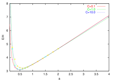
Figure 1: The total Energy per unit Hopf number as a function of $a$, for different values of $C$.

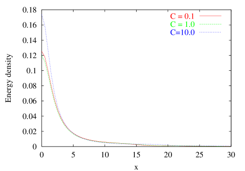
Figure 2: The energy density versus distance for different values of $C$.

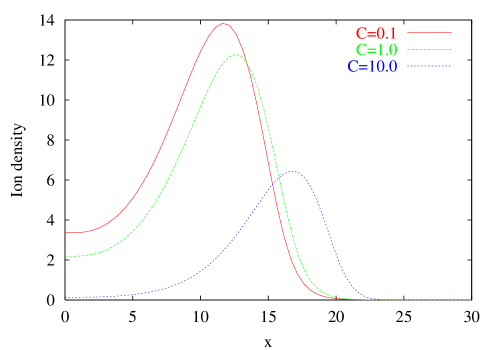
Figure 3: Ion density versus distance at the minimum $a_{C}$ for different values of $C$.

References

- [1] L. Faddeev and A. J. Niemi, Phys. Rev. Lett. 85 (2000) 3416
- [2] E. Babaev, L. Faddeev and A. J. Niemi, cond-mat 0106152
- [3] A.J. Niemi, K. Palo and S. Virtanen, in Yang-Baxter Systems, Nonlinear models and their applications, Proceedings of the APCTP-Nankai Symposium October 1998, B. K. Chung, Q-Han Park and C. Rim editors, World Scientific 1999; Phys. Rev. D61 (2000) 085020
- [4] J. P. Freidberg, Ideal Magnetohydrodynamics, Plenum Press, New York and London 1987
- [5] L. Faddeev, L. Freyhult, A. J. Niemi and P. Rajan physics 0009061
- [6] Y.M. Cho, hep-th 0110076
- [7] L. Faddeev, Qunatisation of Solitons, preprint IAS Print-75-QS70, 1975; and Einstein and Several Contemporary Tendencies in the Field Theory of Elementary Particles in Relativity, Quanta and Cosmology, vol. 1, M. Pantaleo and F. De Finis (eds.), Johnson Reprint 1979
- [8] L. Faddeev and A. J. Niemi, Nature 387 (1997) 58
- [9] J. Gladikowski and M. Hellmund, Phys. Rev. D56 (1997) 5194
- [10] R. Battye and P. Sutcliffe, Phys. Rev. Lett. 81 (1998) 4798; and Proc. Roy. Soc. Lond. A455 (1999) 4305
- [11] J. Hietarinta and P. Salo, Phys. Rev. D62 (2000) 081701; Phys. Lett. B451 (1999) 60
- [12] L. Faddeev and A. J. Niemi, Phys. Rev. Lett. 82 (1999) 1624
- [13] M. Miettinen, A. J. Niemi, Yu. Stroganov, Phys. Lett. B474 (2000) 303