Light Front Models for the Leptons, Bosons, and Quarks

Abstract:

The elementary particles are modeled as harmonic oscillator excitations of transverse U(1) gauge fields propagating at v = c, with open and closed string-like propagation paths. One, two and three node states represent the leptons, bosons, and quarks. We incorporate a twist ($\theta$) for the gauge field components which rotate counterclockwise (L) for the electron, yielding a chiral model. Theta increases by $\pi$ from node to node, making the lepton models SU(2) representations. At nodes the twist may reverse, creating new particle states. For three nodes, twist combinations map the SU(3) color states of the quarks. Generations are modeled topologically by the winding number of the strings. Mapping model E fields to distant observers makes understandable how fractional charges arise for the quarks. These models are 3D slices of spacetime, allowing us to make drawings of particle field conformations. From model particle quantum numbers, new mass relationships are derived.

1 Introduction

The models of the elementary particles described here have drawn from many antecedents. The original Skyrme model [1] has been developed in various directions, for example, by Thirring [2] and Enz [3]. Those efforts inspire one to use symmetries to generate boson and fermion particle states from continuous spacetime fields in low dimensions. The recent and rapid emergence of supersymmetric string models containing BPS states protected from quantum corrections [4] encourages one to believe that relatively simple models may indeed give good representations of elementary particle states. From the quantum gravity side, recent solutions of Einstein Yang Mills Dilaton field equations [5] using axial symmetry have yielded particle states with quantum numbers and geometries similar to those of the models presented here. And from Witten’s [6] development of Chern-Simons topological field theory we have learned that the observable expectation values of relativistic quantum field theories should be topological invariants. This view is reinforced by the demand of relativists that theories of quantum gravity should be diffeomorphism invariant [7]. The real problem is how one can pull all these threads together to weave a consistent theory that represents nature as we find it. The standard model is a large step in this direction. But its shortcomings and the need to move beyond it have been well documented in the literature.

Most current theoretical attacks start with postulated actions or Lagrangians. One then struggles to see what particle states and observables they produce. It now appears that the particle states of interest cannot be reached by applying perturbation theory to known, standard theories. Lacking that methodical approach, one must be intuitive, clever or lucky in guessing new equations as starting points to succeed in finding “nature’s equation”. We choose to reverse that approach, and begin by guessing the solutions that account for known experimental results, and then work back toward the equations. An unfailing guide in building such models is a demand for consistency with all known experimental data, and with cherished theoretical principles. The set of experimental data constraining model building is much enlarged if one demands that all known elementary particles (leptons, bosons, and gluon/quarks) must be consistently described by one coherent model system. This is the goal.

We start with certain biases. Wishing to be “physical”, we confine our modeling efforts to 3 + 1 dimensional spacetime and relevant subspaces. We believe that topological and geometric features of these spaces play a major role in determining the possible and observable particle states. In keeping with this, we work in a semi-classical mode. That is, while keeping in mind quantum demands such as the importance of boundary conditions and wave function nodes, we focus upon classical features dictated by the geometry and topology of the models. Lastly, we believe it is important to be able to visualize the models and their geometric features. To this end, we have developed a depiction system for the models.

Our light front model system for the elementary particles is described below. We believe it succeeds on several levels. (1) It is a consistent system that accommodates all the known elementary particles in terms of a few quantum numbers. Those quantum numbers have logical connections to the geometric, topological and harmonic oscillator constraints that go into the theory. (2) It ties onto the standard model and explicates how the U(1) $\times$ SU(2) $\times$ SU(3) gauge groups arise. (3) It suggests answers to long standing questions such as, “What determines the differences between the three generations of particles?”. (4) It illuminates the origin of electric charge, and makes the fractional charges of the quarks understandable. (5) It provides a depiction system that makes it possible to visualize each particle model. This makes it easy to apprehend the relationships and properties of the different particle states. (6) Studying the model system has suggested to us ways for plotting the experimental rest masses against the model quantum numbers for deriving the functional relationships. The parameters of these mass plots only involve the natural constant $\alpha$ (or e², the electroweak coupling constant) and the electroweak mass $m_{W}$.

The plan of the paper is as follows: In section 2 we give the basic assumptions that go into the model system. In section 3 the depiction method is described and an overview of the particle models is provided by a series of figures. Section 4 provides model details and a discussion of salient features. The way the observed electric charge for each particle arises is described. In section 5 we discuss how the model is extended topologically to treat the higher generations of fermion families. Section 6 summarizes the quantum numbers that specify the particles. Mass relationships are developed in section 7. In section 8 we consider some of the problems of mapping from the spacetime of the particles to that of distant observers. Section 9 presents our summary discussion. There follow two Appendices. The first gives a Mathematica notebook providing calculational details to make explicit features of the electron and quark models that are discussed only qualitatively in the text. The second appendix gives explicit calculations of the electric charges the models exhibit.

2 Assumptions

I. The most basic assumption we make is that all observable particles are transverse quantum U(1) gauge excitations moving at the local speed of light in 3 + 1 dimensional spacetime. These excitations have two orthogonal vector field components which may be identified as electric and magnetic fields in the massive charged particles. In the large, the gauge excitations propagate along geodesics of spacetime as demanded by general relativity. In regions where the excitation is intense, the nonlinear nature of the Yang Mills (and possibly dilaton) equations causes the propagation path to contort and writhe, producing soliton configurations. These are the particles.

II. These excitations are best represented as quantum harmonic oscillators having one node for the leptons, two nodes for the gauge bosons, and three nodes for the quarks. Higher excitations may be possible, but are presently unobserved.

III. The boundary conditions for the excitations are of two types. If the wave functions fall asymptotically to zero at plus and minus infinity (i.e. at a distant emission source and a distant absorber) we have the zero rest mass particles (neutrinos, photons, and gluons). If the wave functions are consistently self-bounded, we have particles with finite rest mass (the electrons, the W and Z, and the quarks).

IV. The orthogonal components of the transverse gauge excitation have a polarization degree of freedom denoted by the twist angle theta. In the development of the models, we found that in every case theta had to change by $\pi$ radians between nodes for the models to be consistent. Hence we postulate that it is a rule of nature that theta must change by $\pi$ radians as the excitation wave function advances from one node to the next. At a node, however, theta becomes undefined. As the wave continues from a node, theta may twist as before, or it may reverse. Which choice is made determines in large measure which particle a given model represents.

V. The non-linear nature of the equations causes the wave to contort and spin about the geodesic, giving rise to spin angular momentum. The spinor particles with boundary condition $\psi(0)=-\psi(2\pi)$ have spin $\hbar/2$ and are fermions. The vector particles with boundary conditions $\psi(0)=+\psi(2\pi)$ have spin $\hbar$ and are bosons.

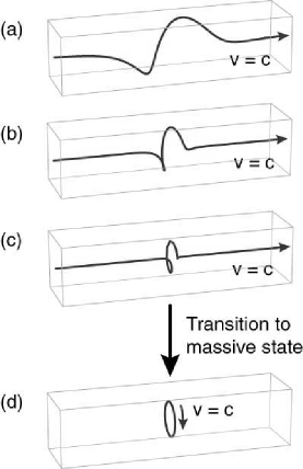
Figure 1: (a) Excitation with zero rest mass propagating at v = c with energy E. (b) Energy = 3E. (c) Energy = 9E. Axial extent of the excitation decreases with increasing E but its curvature grows to keep the angular momentum constant at $n\cdot\hbar$. (d) Excitation undergoes a transition to a self-bounded topology with rest mass. (Propagation is still at v = c, but the excitation remains in the volume element at rest relative to a suitable massive observer.)

VI. In higher energy particles, the propagation path of the excitation may writhe to increase the winding number by an integer number of units compared to the lowest energy particle of the same field configuration. For winding numbers of 1, 2, and 3 we model the observed family generations of fermions.

3 Model Depiction and Overview

The known elementary particles fall into two categories: those with zero rest mass that always travel at v = c, and those with finite rest mass having v $<$ c. Zero rest mass particles include the neutrinos, the photon and the gluons. In the second category we find the massive leptons, the massive gauge bosons, and the quarks. What distinguishes these two categories of particles? As stated in assumption III above, we believe it is a question of boundary conditions for the wave functions of the excitations. Consider a zero rest mass excitation propagating at v = c. Freeze it at an instant of time on the light cone. As depicted in Figure 1a, 1b, and 1c, its wave function must die away smoothly and monotonically at large distances from the location of the excitation. We use the local writhing of the wave function to model the angular momentum of the excitation. Particles have constant angular momentum n$\hbar$ independent of their energy. This is incorporated in Fig. 1.

As the particle energy increases, the longitudinal extent of the excitation decreases, but its curvature increases. Once the threshold energy is passed where everything can fit, a topological transition to a self-bounded state is possible as depicted in Fig. 1d. The excitation now represents a particle with rest mass. The excitation is still propagating at v = c, but since it is self-bounded, its energy density stays in a small volume element of space relative to a real external observer. This is what we mean by rest mass. Of course, transitions to massive particles must conserve quantities like electrical charge. Generally this means one must make a massive particle and its antiparticle at the same time. To summarize, our models of zero rest mass particles will utilize wave functions that go smoothly to zero at plus and minus infinity along the propagation path. Models of particles with rest mass will have wave functions that close back on themselves and are self-bounded. In the standard model, spontaneous symmetry breaking and the Higgs mechanism are used to give mass to otherwise massless gauge particles. Perhaps this is just a hidden way of introducing a topological boundary condition change into the theory.[8]

The model fields to be depicted are moving at v = c. In order to see them as static configurations, we imagine ourselves to be fiducial observers moving at light velocity. That is, we place ourselves on a slice of the light cone centered on the wave function of interest. The x-axis of our image is oriented along the geodesic propagation direction, and we assemble a volumetric image by merging nearby slices in the $+$x and $-$x directions. This is analogous to the way Computer Aided Tomography (CATscan) images are assembled from a series of cross sections. As the propagation path contorts, by assumption I, the gauge field components must remain transverse. As a result, we have two orthogonal components of a twisting field geometry to depict. This is done using Mathematica as a tool for depicting 3D figures with hidden lines removed. (See Appendix 1). On the model figures, it is useful to add an arrow which indicates the direction of advance as the excitation propagates. For twisting fields, this fixes the chirality.

Our models of the massless particles use quantum harmonic oscillator wave functions for both the amplitude of the field components and for the radial displacement of the function baseline from the axial propagation line. For the self-bounded models of the massive particles, we use circular propagation paths and sine functions for the amplitudes. The exact functions used are given in Appendix 1. In the figures, we denote the negative half cycle of the E field vectors using a saturated orange color (dark gray shading for B&W reproduction). The positive E vectors are shown in light orange (medium gray). In a similar manner, for the N and S parts of the B field we use saturated yellow and light yellow shading (light gray and very light gray in B&W reproduction).

Using these conventions, we show a collage of light front models of selected elementary particles in Fig. 2.

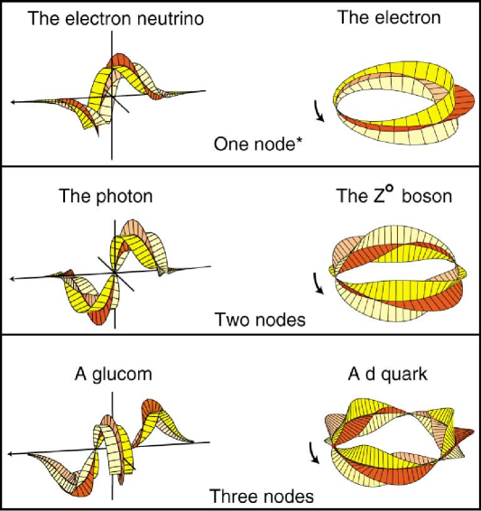
Figure 2: A collage of light front models of selected elementary particles. In the left column are zero rest mass particles with wave functions bounded at plus and minus infinity. In the right column are finite rest mass particles having self-bounded wave functions. A glucom is a gluon component. These are first generation particles. * We count one node at infinity.

They are organized from top to bottom by the number of harmonic oscillator nodes in the particle wave function. The number of nodes emerges as one of the key quantum numbers. Specifically, for n = 1 we model the leptons, for n = 2 we model the gauge bosons, and for n = 3 we model the quarks and glucoms (which are gluon components to be discussed later). In keeping with Assumption IV, the component field vectors twist about their propagation path by $\pi$ radians as the wave front moves from a given node to the next in the direction of the arrows. No antiparticles are shown in Fig. 2, but they can easily be imagined. To obtain the antiparticle of a given model one reverses the direction of twist rotation as the fields advance. This is equivalent to a PC transformation. It reverses the chirality and the charge exhibited by the model.

In these models, there are three different features with periodicity. The U(1) gauge fields are periodic. The twist angle theta is periodic. And in the massive models, once around the circle is a geometric period. The way these periodicities correlate differs from particle model to particle model, and in fact determines the electric charge exhibited. The story is simple but intriguing for the n = 1 electron. As the number of nodes rises, the possibilities increase, until we reach the quarks with their several charges and multiple colors. Let us begin with the simple case first.

4 Model details and salient features

4.1 The electron model

An oblique view of the electron model is shown at the upper right in Fig. 2. The gauge fields are represented simply by orthogonal sine waves propagating around a ring, twisting as they go. The key feature is that the ring circumference is made equal to half the electromagnetic wavelength. In similar manner, we make once around the ring produce 1/2 twist, that is, $\pi$ radians. These are considered quantum requirements which combine to produce a stable soliton field configuration that models the electron. As a geometric structure, it has some exceptional properties. The half twist for once around makes each vector field into a Möbius strip. Normally, such a manifold is non-orientable. But when the geometry inversion is combined with the electromagnetic field reversal each time around, the field becomes oriented and self-bounded. Consider the magnetic field shown in yellow (light gray). Starting at the node, follow the wave function twisting around the ring as it goes through its maximum and back to zero. Let this represent the north half cycle of the field. Continuing around, the field reverses and we trace the light yellow (lightest gray) wave function through its maximum and back to zero. Let this represent the south half cycle of the field. At this point we have completed one full cycle of magnetic field variation, and also one full 2$\pi$ twist about the ring. So both the wave function and the twist are ready to repeat their cyclic variation. In other words, they are consistently self-bounded. Now look at the resulting geometry. Even though the magnetic wave function is alternating N to S in a cyclic way, the N half of the field is always on the top side of the ring. In like manner, the S part of the field is always on the bottom side of the ring. Recall that this is a light front model with the fields propagating around the ring at v = c. From far away, a real, massive observer would see only the time averaged resultant of the field motion. He or she would see a magnetic dipole. Now focus on the orthogonal fields shown in orange (dark gray). A similar geometric effect occurs when the twist inversion is combined with the cyclic field inversion. In this case one half of the field variation (which we choose to call the negative half cycle since we are modeling an electron) always remains external to the ring. The other half cycle always remains internal to the ring. As before, we start with an electromagnetic field component that is cyclically varying from plus to minus, and end up with a time averaged field that is minus external to the ring, and plus inside. What would a distant real observer see? We claim he can see only the portion of the field external to the ring, and consequently he sees a negatively charged particle. The fields internal to the particle are hidden from view. Why? The ring is the locus where the fields are moving at the local speed of light. This is very like a Kerr black hole which possesses an event horizon. External observers cannot see any phenomena that occur inside such a horizon. We take this seriously, and consider our model of the electron to be a soliton with an extreme Kerr geometry. Such models (excluding the twist) have been invoked before in the context of heterotic string solitons[4].

We note that once around the propagation ring corresponds to only half the U(1) period. So the wave must go around again to make one complete wavelength of the field. Requiring a 4$\pi$ revolution for a symmetry operation is the hallmark of spinor behavior, and this brings the fundamental representation of the SU(2) group into our models. It is known from experiment that the electron neutrino and the electron are chiral particles. Using standard conventions, they are left handed. Our models have an internal chirality because of their helical conformations. If we label them properly, they are left handed. Further, as noted above, their antiparticle models are right handed, in accord with experiment.

We need to find a way to take the fields specified for the light front models and deduce the magnitude of charge and dipole strength that they represent to a real, distant observer. How does one measure the charge contained in a volume of space? One integrates the field strength emerging from a sphere containing the “charge” and uses Gauss’ law to determine the number of charges inside. We will do likewise for the models, using the following algorithm. The E field vectors emerge from the ring at all angles, but we argue that only the component of the field in the equatorial plane of the ring is strictly radial, and capable of escaping the event horizon. So we project each E vector onto the equatorial plane and integrate through one complete cycle, keeping in the integral only those components that are directed outwards. A visual way of doing this is to look down onto the top view of the model, and count only the field external to the ring. This calculation for the electron model of Fig. 2 yields the result of $\pi$, as detailed in Appendix 2. So we normalize the integral, multiplying by $-1/\pi$. This algorithm now yields the charge of $-1$ for our electron model. Consider this a calibration of the charge exhibited by the model. We will use this same algorithm to assess the charge exhibited by all the other particle models. One check we can apply at once is to see if the E field, when projected onto the polar axis and integrated for a complete cycle gives any result. The result is zero. So there is no polar dipole associated with the E field. Henceforth we will use this as our definition for model fields that are to be labeled E. We treat the axial fields in a similar way, but obtain a different result. The field atop the ring , when projected onto the polar axis and integrated around yields +$\pi$. The bottom field yields $-\pi$. Both axial fields give zero for their integrated equatorial projection. Thus they represent the field of a magnetic dipole, and we label them B.

4.2 The boson models

We now turn to the $Z^{o}$ model depicted in the middle of Fig. 2 on the right. The gauge field components have two nodes for once around the ring. That corresponds to one complete period of the U(1) field, so we no longer have a spinor. Nevertheless, in Fig. 2 we show the boson fields going twice around; this makes the resulting picture directly comparable to the fermion depictions. What is special is that the twist direction reverses at each node. Thus if we start with a counterclockwise twist (call it L) in going from the node near the arrow, we change to a clockwise twist (call it R) at the next node. We denote this twist pattern as LR. Had we started noting the twist pattern at the next node, the pattern RL would be obtained. The starting node is arbitrary so these two patterns are equivalent. Both produce a neutral particle model. Our algorithm for assessing the charge exhibited by these models has a visual counterpart. If one takes a top view of the models, the fields are projected onto the equatorial plane. One can then observe how the + and $-$ parts outside the ring add up. This is shown in Fig. 3.

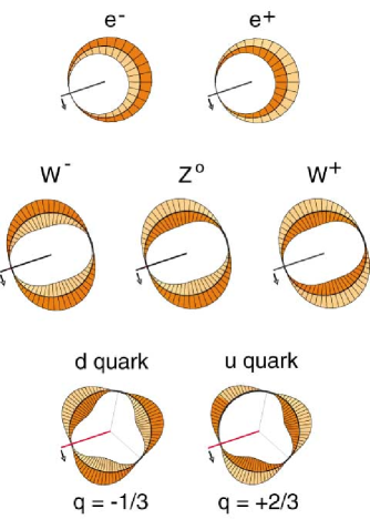
Figure 3: Projection of particle model E fields onto the equatorial plane. Distant observers see the field integrated once around, but see only the portion external to the dark circle - which represents an event horizon.

For the $Z^{o}$ it can be seen that the $-$ field on one half of the ring cancels the + field on the other half. In Fig. 3 the B fields have been left out for clarity in being able to assess the electric charges. Finishing out the massive bosons, we find that the LL twist pattern makes the negative parts of the field add to give a model of the $W^{-}$. And the RR twist pattern gives the $W^{+}$. The photon model can conceptually be obtained from the $Z^{o}$ model by opening up the latter at one of its nodes and pulling the ends out to plus and minus infinity. This gives a model as shown on the middle left of Fig. 2. Our photon model has a center of antisymmetry. This means that the photon is its own antiparticle, a fact consistent with the experimental observation that a sufficiently energetic photon can materialize into any particle-antiparticle pair.

4.3 The quark models

In the n = 3 particles, there are more ways the twist degree of freedom can combine with the U(1) periodicity. This produces more particle states, which shows up experimentally in that quarks come in two charge states (the + 2/3 u quark and the $-$1/3 d quark), and in three colors. We are challenged to model all these states in a consistent way within our system. This can be done as follows. At the bottom right of Fig. 2 we see the model of a d quark of some particular color. We know it is a d quark from its electric charge of $-$1/3. That was determined by our projection algorithm, visualized at the bottom of Fig. 3. There for the d projection we see that the E field is broken into three pieces by the nodes. Two of the pieces cancel, leaving the third piece to provide the average field seen by distant observers. How does this come about? As with the electron model, we have to go around the ring twice to have the U(1) field advance an integer number times 2$\pi$ so it can consistently repeat. So we have a spinor wave function once again. The twist degree of freedom therefore has six nodes at which it may reverse, or not. The twist pattern that yielded the d quark of Figures 2 and 3 was LLR-LLR. Note that there are two more equivalent patterns which also yield a $-$1/3 charge d quark. They are LRL-LRL and RLL-RLL. These patterns are truly degenerate models in that they differ only in the origin node one chooses for writing down the pattern. This is our model representation of color. Call one pattern red, and the other two blue and green. For an isolated quark, the phase denoted by color does not matter. But when two or three quarks combine to form hadrons, their relative phases do matter. It is then that color matters. The key thing to notice about these d quark twist patterns is that they are the same each time the excitation goes around the ring. Suppose that on the second time around the ring, one of the twist directions changed from what it was the first time around? We get a +2/3 charge u quark. The u quark projection shown in Fig. 3 came from the twist pattern LLR-LLL. As can be seen, the E field breaks up into three pieces at the nodes. But this time one piece cancels itself out, leaving the other two to add up to 2/3 of a charge. As before, we have three degenerate twist patterns that lead to the same charge state. For the u quark, the other two are LRL-LLL and RLL-LLL. Again we can assign these states color names. These threefold possibilities for each charge state bring the fundamental representation of the SU(3) group into our model.

4.4 Gluons and Glucoms

The n = 3 zero rest mass particle shown at the lower corner of Fig. 2 does not seem to correspond to any presently known particle. However, it may be considered to be a gluon component in the following sense. In standard QCD, the gluons are bicolored objects of spin one derived from the adjoint representation 8 of SU(3). They can be considered to be made up from two single colored objects from the defining representation 3 of SU(3). We call these gluon components glucoms. Our unassigned n = 3 particle fits well as a representation of a gluon component. The possible twist patterns LLR, LRL, and RLL represent the three color states of the glucom. The corresponding anticolor glucoms are RRL, RLR, and LRR. One gluon emission by a quark is then equivalent to emission of a glucom and an antiglucom together. One does not usually break gluons down this way in standard theory. Nevertheless, this description seems to fit. In fact, we believe that glucoms may one day be observed and found to play in important role in some physical phenomena.

5 Higher Generations of Fermion Families

In model terms, how shall we account for the experimental observation that the leptons and the quarks come in three generations? The nature of the excitation involved has been a puzzle of long standing [9]. A hint comes from noting that in the electron model the vector fields are analogous to a closed twisting ribbon. Such ribbons have another degree of freedom; they can writhe to make the centerline of the ribbon non planar. So far, the electron model has a plane circular propagation path with curvature, but no torsion.

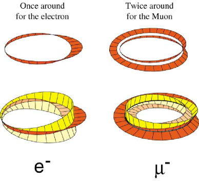
Figure 4: The electron has a field configuration with a half twist for each $2\pi$ revolution of its wave function. The muon has a 3/2 twist for each $2\pi$ revolution. But by writhing back upon itself, this is equivalent to a $4\pi$ revolution of the wave function with only a half twist. In this view, the muon goes twice around, giving a winding number of two. This restores the field geometries so they exhibit the same charge and magnetic moment as the electron. This makes the muon just a heavy electron, as it is in nature.

If at higher energy torsion became appreciable, then the propagation path would begin to have non-zero writhe. We postulate that quantum increases in writhe account for the excited states that higher particle generations represent. Yet writhe seems not the proper variable, as it is geometric, not topological. Closed ribbons in 3D obey a simple relation: Lk = Tw + Wr [10], where Lk is the linking number of the two edges considered as separate curves in space. For a closed ribbon, Lk is a topological invariant. But the ribbon twist (Tw) and writhe (Wr) can trade off with each other. However, for a closed ribbon with a central obstruction, the writhe can no longer be changed and it becomes topological. In such a case the writhe can be given a more physical representation and name; the writhe plus one is the winding number, telling how many times the ribbon winds around the obstruction before closing. This is a topological invariant which seems a candidate for our generation quantum number.

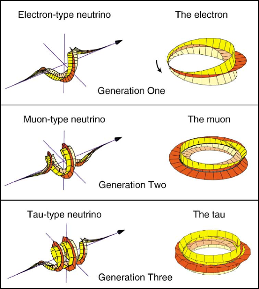
Figure 5: Light front models for three generations of leptons. Generations one, two and three are distinguished by winding numbers of one, two and three respectively. All the particles shown have one node and one half twist in each field component.

We take the interior of the horizon in our model to represent the interior of the Kerr spacetime geometry - a special region, which is an obstruction around which the field winds. Exploring this possibility, we assign a winding number of one to the electron, two to the muon, and three to the tau. The way this translates into model field geometries is shown in Fig. 4 where we retain the one node and half twist features of the electron, but increase the winding number to two to obtain a muon model.

When we apply our algorithm of projecting and integrating the E field around to compute the model charge, we find it comes out minus one, just as for the electron. Increasing the winding number to three yields a tau model that also exhibits a model charge of $-$1. This same idea can be applied to the electron type neutrino model to yield the corresponding second and third generation neutrinos. In Fig. 5 are given depictions of the lepton particles for all three generations, using the winding number approach.

It is clear that the same idea may be applied to the quark models, but we do not show the resulting models. In that case having three nodes, the field geometries become so complex that the depictions are confusing and not very useful. This approach to modeling the generations of particles appears promising in that: (1) it is a natural topological extension of our light front models, (2) it is based upon a quantum number that is a topological invariant well known in other contexts (quantum hall effects), (3) the models for higher generation leptons exhibit the same electrical charge as the first generation models, and (4) it uses a mechanism that works equally well for the leptons and the quarks. But there is a more compelling reason to believe that there is some truth in this description. Witten [13] has shown that the expectation values of observables depend upon the writhe of framed links in a topological field theory derived from a Chern-Simons action. When we plot the lepton masses for all three generations in that way (see below), we obtain a beautiful linear plot whose parameters are given by the weak coupling constant $e^{2}$, and the weak mass scale $m_{W}$. No adjustable parameters are needed. This is discussed below.

6 Quantum Numbers

We have introduced several quantum numbers that in model terms distinguish one elementary particle from another. To bring them into focus, we summarize them and their significance in Table 1.

Table 1. Quantum numbers for specifying the different elementary particles. Quantum Numbers for All Particles Symbol Allowed
Values Name Significance b 0,1 boundary type b = 0 for zero rest mass particles
b = 1 for particles with rest mass h +1, 0, $-$1 handedness h = +1 for particles
h =   0 for self-conjugate particles
h = $-$1 for antiparticles n 1,2,3 nodes n = 1 for leptons
n = 2 for gauge bosons
n = 3 for quarks and glucoms $\mathbf{n_{w}}$ 1,2,3 winding number $\mathrm{n_{w}}$ = 1 for 1st generation particles
$\mathrm{n_{w}}$ = 2 for 2nd generation particles
$\mathrm{n_{w}}$ = 3 for 3rd generation particles Quantum Numbers for $n>1$ Particles t +1, $-$1 twist splitting t = +1 and n = 2 gives W particles
t =  $-$1 and n = 2 gives the $Z^{o}$
t = +1 and n = 3 gives u, c, or t quarks
t =  $-$1 and n = 3 gives d, s, or b quarks Quantum Numbers for $n>2$ Particles c 1,2,3 color h =   1 and c = 1 gives red
h =   1 and c = 2 gives green
h =   1 and c = 3 gives blue
h = $-$1 and c = 1 gives antired
h = $-$1 and c = 2 gives antigreen
h = $-$1 and c = 3 gives antiblue

A dream of ours has been to have a grand computer program that would take values of these quantum numbers as input, and then produce as output a light front model depiction of the particle specified. In fact, we find it more convenient to have several programs (one for the massless particles, another for the massive particles, etc.) Still, the dream challenges us to come up with a minimal set of quantum numbers that can uniquely specify each of the known particles. In addition we seek quantum numbers that have an obvious physical, geometric or topological meaning. Here is our set. First we choose a quantum number b whose function is to specify the type of boundary condition the wave function must satisfy. Its value determines whether our chosen particle does or does not have rest mass. Next we specify a chirality or handedness factor h; it specifies whether we are dealing with a particle or antiparticle. The special value h = 0 is used for particles like the photon that are their own antiparticle. The choice between leptons, bosons, and quarks is made by specifying n, the number of nodes in the gauge wave function. Lastly we choose the particle generation by giving the winding number $\mathbf{n_{w}}$ (note that bosons have only the $\mathbf{n_{w}}$ = 1 generation for reasons discussed below). These are the basic quantum numbers that apply to all the particles. When n $>$ 1, we need a quantum number to account for the splitting between the W and $Z^{o}$, and also between the u and d quark sectors. In the models, the feature which distinguishes these particles is the total twist of the gauge field for one complete cycle of the U(1) field. So we define a twist splitting quantum number t. In a similar manner, when n $>$ 2, we need a quantum number to specify the twist permutation pattern. So for the quarks we define a color quantum number c. The allowed values for these quantum numbers are given in Table 1. We not only use these quantum numbers for specifying particles to our programs, but also will use them in the particle mass relationships discussed below.

7 Particle Mass Relationships

The masses of the three generations of leptons are well known from experiment ($m_{e}$ = 0.511 MeV, $m_{\mu}$ = 105.7 MeV, and $m_{\tau}$ = 1777 MeV) [11], but they have never been understood theoretically. It is clear that the masses rise rapidly and perhaps exponentially with generation number. We, and many others, have tried fitting them with an exponential relationship. See reference [12] for a recent attempt. The results of those attempts have never really been satisfactory. The trouble was that no one had any idea what kind of excitation was involved in going from the first generation to the second or third. But in the context of the light front models, we do have an idea. It is the increasing writhe (or winding number) that leads to the higher generations. With that as a hint, we ask how such a thing might arise in quantum field theory.

Our models begin in 3 + 1 dimensional spacetime. But by assumption I, the gauge excitations are restricted to be transverse. This reduces their spacetimes to 2 + 1 dimensions. So the theory we seek should be a 2 + 1 dimensional quantum field theory whose observables (like rest mass) are functions of topological invariants. The natural choice is a Chern-Simons (CS) topological quantum field theory (TQFT), as wonderfully explicated by Witten [13]. We are further encouraged in this direction when the writhe and winding number of the gauge fields emerge from such a theory as a key variables.

To apply CS theory, one must choose an oriented three manifold and a gauge group. For application to our models, we choose $R^{3}$ for the manifold and U(1) as the gauge group. (Recall that the expected SU(2) group for fermions enters the models later.) These choices lead to the simplest possible CS action:

$$\mbox{$S_{CS}$}=\frac{k}{4\pi g^{2}}\int_{R^{3}}A\wedge\,dA$$

where A is the vector potential, k is the level (which we will set to one to obtain the lowest state), and g is the coupling constant. For the case of a transverse U(1) vector field propagating around an $S^{1}$ path embedded in $R^{3}$ with blackboard framing (no twists), the CS action equates to the Gauss’ self-linking number or writhe of the field multiplied by the scale factor. This is shown explicitly in [14]. Witten [13] went farther, showing that the Feynman path integral of the Chern-Simons action over all gauge orbits around the $S^{1}$ link C yields the partition function of the theory - a topological invariant. Next one defines a Wilson line operator $W$ which gives the holonomy of the connection integrated around the cyclic path:

$$\mbox{W}=\mbox{P}exp[\int_{C}A\>dA]$$

Combining these in the path integral, Witten showed

$$\langle\mbox{vev}\rangle\>=\int DA\>exp\>[\mathrm{i}S_{CS}]\>\prod_{i}\>W_{i}=e^{\Lambda\cdot\mathrm{writhe}}\>[\mbox{Jones Polynomial}(C_{i})]$$

The result is a topological invariant - the vacuum expectation value (vev) of the operator $W=\prod_{i}\>W_{i}$. (We have omitted from the equation above the partition function that serves as a normalizing factor. As will be seen below, we let the data plot determine it, which in our case becomes the mass scale factor.)

Witten showed that this vev is also given by the well known Jones polynomial invariant $\langle\mbox{J}\rangle$ for the link multiplied by a writhe factor that takes into account the conformation of the embedding of the framed $S^{1}$ link in $R^{3}$. In knot theory, this combination goes under the name of the Kauffman bracket for certain choices of its variable.

We hope to apply this to the present models by considering the experimental rest masses of the $e$, $\mu$, and $\tau$ leptons as observables depending upon some function of the vev of the applicable Chern-Simons TQFT. But there are subtle features to be dealt with.

First, the framed link invariant given by the CS path integral is $\langle\mbox{K}\rangle$, the Kauffman Bracket [15], whose framing dependence is made explicit as a writhe prefactor times the Jones polynomial, thus $\langle\mbox{K}\rangle\>=(q)^{\mathrm{writhe}}\langle\mbox{J}\rangle$. The quantity q is the Chern-Simons phase $exp(i\pi/k)$ for the U(1) case. For the level k = 1, q = $-1$. Next, there is an issue of signs [16]. To give the vev, the Kauffman bracket must be multiplied by $(-1)^{\mathrm{winding\>number}}$. As was mentioned earlier, for planar projections, the winding number is just the $(\mathrm{writhe}+1)$. Thus we get the curious equation:

$$\langle\mbox{vev}\rangle\> = (-1)^{\mathrm{writhe}}\cdot(-1)^{\mathrm{writhe}+1}\prod_{i}\>\langle J_{i}\rangle$$

$$= -\prod_{i}\>\langle J_{i}\rangle$$

The surprising effect of all this is that the writhe prefactor arising from the CS action has no effect for our level k=1 U(1) gauge field other than to introduce a minus sign. What is left in the vev is the product of Jones Polynomials, one for each loop the field makes. This is relevant since for the electron model we go once around; for the mu model, twice around, and three times for the tau. These Jones Polynomials are usually normalized to unity for the unknot. But they arise from the Wilson loop operators. In our fermion case, due to the half twist of the fields as they go once around, they have traversed only half of the field cycle. If we normalize to a complete field cycle, then each loop yields a holonomy of 1/2. In our model for the generations, the winding number of each model gives the number of loops; it also gives the number of factors of 1/2 in the vev. By this argument, we obtain

$$\langle\mbox{vev}\rangle\> = -\left(\frac{1}{2}\right)^{n_{w}}$$ (1)

where $n_{w}$ is the winding number.

A last complication is that this TQFT Expectation Value has been derived for the 2 + 1 spacetime of our models on the light cone. But we make our observations asymptotically far away in a flat 3 + 1 spacetime. There must be a mapping from one to the other that makes our observable (we focus on mass) some function of the TQFT Expectation Value. We take our clue from Hawking and Ellis [17], who prove that timelike paths from asymptotic infinity to the light cone constitute an exponential map. If we assume an exponential relationship, then we can write a possible lepton mass relation as

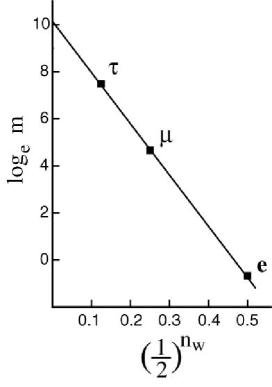
Figure 6: Mass plot for the leptons. On the abcissa $n_{w}$ is the gauge field winding number with $\mathbf{n_{w}}$ = 1, 2, 3 for the first, second, and third generation particles respectively. All masses are in MeV. The line is theoretical from equation (4). It has a slope of $-$2/(4$\pi\alpha$) and an intercept of log ($m_{w}$/$\pi$). where $m_{w}$ is the mass of the W boson in MeV.

$$\frac{m}{m_{0}}=exp\left[-a\left(\frac{1}{2}\right)^{n_{w}}\right]$$ (2)

or, in logarithmic form

$$\log m=-a\left(\frac{1}{2}\right)^{n_{w}}+\log m_{0}$$ (3)

where $m_{0}$ is the mass scale factor, $a$ incorporates the coupling constant of the CS action, and $n_{w}$ is the winding number. The validity of this functional form can be tested by plotting $\log m$ versus $\left(\frac{1}{2}\right)^{n_{w}}$ with $n_{w}$ = 1, 2, and 3 for the $e$, $\mu$, and $\tau$ leptons respectively. Those winding number values are derived from our light front models of the lepton generations as was described in Section 5. If the functional form is correct, we should get a linear plot whose slope is $-a$ and whose intercept gives $\log m_{0}$. We have done this (expressing all masses in MeV) as shown in Fig. 6.

The result is a good linear plot. Surprisingly, the value of $a$ from the slope is equal to 2/(4$\pi\alpha$), where $\alpha$ is the fine structure constant (1/137). In natural units, 1/(4$\pi\alpha$) is $e^{2}$, the electromagnetic coupling constant. In like fashion, the plot intercept gives $m_{0}=\frac{m_{W}}{\pi}$ where $m_{W}$ is the mass of the W boson (80,430 MeV). Using these values for $a$ and $m_{0}$, gives the lepton mass formula

$$m_{i}=\left(\frac{m_{W}}{\pi}\right)exp\left[-\frac{2}{4\pi\alpha}\left(\frac{1}{2}\right)^{n_{w_{i}}}\right]$$ (4)

where for $i=1,2,3$ the winding number $n_{w_{i}}=1,2,3$ for the $e$, $\mu$, and $\tau$ leptons respectively.

The line plotted in Fig. 6 is that given by equation (7.4). Its goodness of fit can be judged by the calculated lepton masses: $m_{e}$ = 0.47 MeV (7.8% low), $m_{\mu}$ = 110 MeV (3.8% high), $m_{\tau}$ = 1677 MeV (5.6% low). If we count $\alpha$ and $m_{W}$ as relevant constants of nature, then this representation has been obtained with no adjustable parameters. We take the linear fit, and the appearance of the natural constants as indicators that our approach is on the right track. This kind of relationship can be extended to include the quarks, but those cases are more complex and require new approximations. That work will be described in a separate paper.[18]

We should comment upon the gauge bosons, however. Experimentally, the bosons do not show generational behavior. Why not? In the context of our CS TQFT picture let us focus on the Wilson loops for the bosons. They integrate over one complete cycle of the field in going once around the loop. The positive half cycle cancels the negative half cycle giving a zero result. Thus we replace the 1/2 in equation (1) with zero. The result for bosons is that their vevs no longer depend upon the winding number.

8 Spacetime Mappings

Several times above, we have alluded to the need for mapping expectation values that arise in the vicinity of particle horizons onto the spacetime of distant real observers. For measuring electric charge, distant observer measurements must time-average over the cyclic motion of the fields. But there is a spatial mapping that is not trivial. If electrons are really tiny, rapidly rotating black holes of Kerr geometry as our models postulate, then the spacetime just outside their horizon is dragged into rotation as well. Also, the E field leaves the electron predominently in its equatorial plane. How can it be that a distant, massive observer sees a nonrotating radial field from what appears as a point charge? We depict this problem in Fig. 7, using a cartoon drawing.

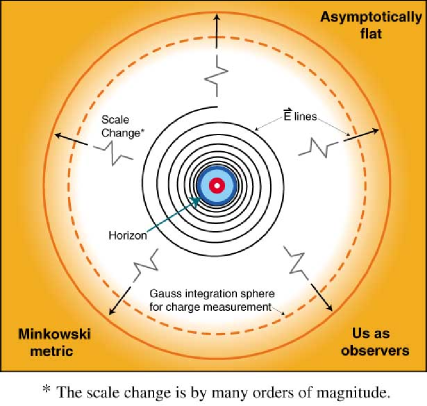
Figure 7: A cartoon depiction of a static mapping from the Kerr geometry of the electron E field onto the Minkowski geometry of an observer asymptotically far away. We are looking down onto the equatorial plane of the particle.

The way rotating fields can map to stationary points has an answer long known in physics. It is the spinor property of entangling its fields upon a 2$\pi$ rotation and then untangling them upon a further 2$\pi$ rotation. This is nicely illustrated by Misner, Thorne and Wheeler in [19]. There is even a U. S. Patent [20] for a device that accomplishes this trick on a continuous basis. But it works only for spinors such as fermions. Bosons like the W and the $Z^{0}$ are not spinors. What about them? This leads us to a speculation about a troubling observation.

Why are the first generation fermions very light while the simplest massive bosons very heavy? The electron is extremely light, with mass of about .5 MeV. The u and d quarks have mass less than 10 MeV. In contrast, the W boson has a mass of over 80,000 MeV. The difference cannot be ascribed to the difference in node numbers, for the light electron and quarks have node numbers of one and three respectively, while the heavy bosons have node number two. We speculate that it is the mapping of fields propagating to distant observers that gives rise to the huge difference in observed masses. All of the particles, as modelled here, are sources of twisting gauge fields propagating outward. These fields carry energy and contribute to the energy momentum tensor that distant observers use to measure mass. For the fermions, the twist energy gets averaged over only a 4$\pi$ rotation of the model fields due to the 4$\pi$ symmetry property of spinor fields. But there is no such limited averaging for the bosons. They do not possess the spinor symmetry property. For the bosons, the twist gauge field energy gets averaged over a large number of model rotation cycles. How to specify this is not clear. Yet the qualitative difference between the fermion and boson cases is clear. We will not pursue this farther here.

9 Discussion

Now that the models have been developed and presented, it seems a good time to reconsider some of the assumptions that went into them. As illustrated in Fig. 1, we postulated that the propagating gauge fields would writhe about the geodesic propagation path in regions where the excitation was intense. How might this arise? One can always speculate about nonlinearities in the field equations but we can be more specific. We invoked a Chern-Simons term in the action for a TQFT to explain the mass plot of Fig. 6. Physically considered, the CS form is a generator of torsion in the following sense. A propagating gauge field sweeps out a space curve whose direction at a point is given by the tangent to the curve. The gradient dA defines the normal to the curve at the same point. This establishes a plane in which the space curve may exhibit curvature. The wedge product with A defines the binormal direction which is perpendicular to the plane just described. Motion of the propagating field in the binormal direction exhibits torsion. In view of this, we ascribe the torsion of the paths shown in Fig. 1 to a CS term in the Lagrangian. In fact, the CS term must be the dominant term in the Lagrangian in view of the excellent fit to the lepton masses shown in Fig. 6. The fit is not perfect, however. This suggests to us that there are Maxwell terms and perhaps others we have ignored. There may also be quantum corrections we have left out. Nevertheless, it appears that the Chern-Simons term dominates.

As the light front models were being developed, it became clear that the twisting of the fields about their propagation direction was a key feature. First for the electron model, and then for the bosons and quarks the change of twist by $\pi$ radians from one node to the next was required to give reasonable model geometries. Since this appeared in every case, we have elevated it to the status of a natural law as stated in assumption IV. Perhaps the twist degree of freedom should be made the basis of the gauge field. It exhibits U(1) group behavior. And the electromagnetic field could be considered to arise as the gradient of the $\theta$ field. The fact that CS TQFT assigns an important role to the twist of framed links representing the gauge fields also suggests one should pursue these possibilities.

The modeling of leptons, bosons and quarks as 1, 2 and 3 node harmonic oscillator states of the gauge field immediately suggests that states with 4, 5, and 6 or more nodes might be made with accelerators of higher energy than those presently available. This theory, unlike some, does not predict a desert unpopulated with states until one approaches the Planck energy. The n = 3 states (quarks) show a much richer phenomenology than the n = 1 states (leptons). One might expect the n = 5 states to be richer yet.

These models cast new light upon whether magnetic monopoles can exist or not. In looking at the electron model of Fig. 2 it would seem that a particle with magnetic charge could be made by merely rotating all the fields $\pi$/2 radians about their propagation direction. Then the yellow (light grey) fields would become radial and the orange (dark grey) fields would become polar. Yet from a distant observers point of view, nothing has changed. He still sees a particle with a radial gauge flux that looks like an electric field. And he sees a dipolar field that looks magnetic. The point is that the orthogonal components of the gauge field are completely equivalent in the massless particles. In the massive particles they become different because of the symmetries they are forced to adopt. We label the radial field E and the polar field B. Given this viewpoint, our models suggest that magnetic monopoles cannot be made. This is in keeping with the experimental fact that they have never been observed in a repeatable way despite many searches.

As was shown in Fig. 2, we had to postulate an as yet unknown particle that is the n = 3 counterpart to the neutrino. We tentatively called it a glucom as it appears as a gluon component. We suggest that this is a real particle yet to be discovered. One can speculatively think of several places where glucoms might play a role in physics and cosmology. Suppose that in the core of the sun some of the newly formed neutrinos could combine with photons to make glucoms. They likely would not be detected by present solar neutrino detectors. This could contribute to the observed solar neutrino deficit. Glucoms could also make up some of the dark matter of the universe. We will not pursue these speculations here.

The elementary particles as modeled here represent a new and lower level in our understanding of the structure of matter. It appears to be a level with many interesting structures that are both geometric and topological in nature. We suggest that the structures be called geotopes. One can only hope that geotopic structure theory will need to be extended to handle the n = 4, 5 and 6 geotopes.

10 Appendix 1. Mathematica Program for the
Quark and Electron Light Front Models

(* This program depicts a light front model of the d quark with the
setting nodes = 3. It can also depict the electron model if the value
is changed to nodes = 1.

The model is specified using toroidal coordinates of scale
baseRadius.  There are two plotting parameters, t and v. The angular
parameter is t, with range {t,0,4Pi}. We make the angular parameter
go twice around to accommodate spinor wave functions. The radial
parameter is v, with range {v, 0, maxMinorRadius}. The positive and
negative parts of the E field are rendered using light orange and
intense orange colors respectively. The N and S parts of the B field
use yellow and light yellow. In toroidal coordinates, the fields are
defined by:

Plus E field  (orange):           North B field ( yellow):
r = v Sin[nodes*t/2]              r = v Sin[nodes*t/2]
theta =twists*t                   theta = twists*t/2 + Pi/2
phi = t                           phi = t

Set pcFactor to +1 for a particle, or to -1 for an antiparticle *)

nodes = 3; twists = nodes/2; pcFactor = +1;

baseRadius = 3.0; maxMinorRadius = 1.0;

If[nodes==1, ch=+1, ch=-1]; (* Sets correct chirality for electron
case *)

ToroidalToXYZ[chirality_,r_,theta_,phi_] [hueColor_,saturation_] :=
  {(baseRadius + r Sin[-chirality*pcFactor*theta]) Cos[phi],
  (baseRadius + r Sin[-chirality*pcFactor*theta]) Sin[phi], r
  Cos[-chirality*pcFactor*theta], SurfaceColor[Hue[hueColor,
  saturation, 1.0]]}

Field[chirality_,sign_,start_,end_,orient_,hue_,sat_] :=
  ParametricPlot3D[ ToroidalToXYZ
  [chirality,v*(sign)*Sin[nodes*t/2],twists*(t+orient),t] [hue,
  sat]//Evaluate, {t,start, end},{v,0.019,maxMinorRadius}, Boxed ->
  False, PlotPoints->{30,2}, ViewPoint->{1.087, 4.108, 2.2},
  LightSources -> {{{1.,0.,1.}, RGBColor[1,1,1]}, {{1.,1.,0},
  RGBColor[1,1,1]}, {{0.,1.,1.}, RGBColor[1,1,1]}, {{-1.,-1.,1.},
  RGBColor[1,1,1]}}, DisplayFunction->Identity];

orange1 =     Field[+1, -1, 0,     2Pi/3, 0, .03, 1];
orangelite1 = Field[+1, +1, 0,     2Pi/3, 0, .03, 0.75];
orange2 =     Field[+1, -1, 2Pi/3, 4Pi/3, 0, .03, 1];
orangelite2 = Field[+1, +1, 2Pi/3, 4Pi/3, 0, .03, 0.75];
orange3 =     Field[ch, -1, 4Pi/3, 2Pi,   0, .03, 1];
orangelite3 = Field[ch, +1, 4Pi/3, 2Pi,   0, .03, 0.75];

OrangeField = Show [orangelite1,orangelite2,orangelite3,
  orange1,orange2,orange3, DisplayFunction->Identity];

yellow1 =     Field[+1, -1, 0,     2Pi/3, Pi, 0.2, 1];
yellowlite1 = Field[+1, +1, 0,     2Pi/3, Pi, 0.2, 0.75];
yellow2 =     Field[+1, -1, 2Pi/3, 4Pi/3, Pi, 0.2, 1];
yellowlite2 = Field[+1, +1, 2Pi/3, 4Pi/3, Pi, 0.2, 0.75];
yellow3 =     Field[ch, -1, 4Pi/3, 2Pi,   Pi, 0.2, 1];
yellowlite3 = Field[ch, +1, 4Pi/3, 2Pi,   Pi, 0.2, 0.75];

YellowField = Show[yellowlite1,yellowlite2,yellowlite3,
  yellow1,yellow2,yellow3, DisplayFunction->Identity];

axis = Graphics3D[Line[{{0,0,-5},{0,0,4}}]];

redLine = Graphics3D[ {RGBColor[1,0,0], Thickness[.01],
  Line[{{0,0,0},{3.8,0,0}}]}];

Particle = Show[OrangeField,YellowField,axis,redLine,
  ViewPoint->{1.087, 4.108, 2.2}, Axes->False, PlotRange->All,
  DisplayFunction->$DisplayFunction]

(* Graphic deleted. See Fig. 2 at the bottom right for depiction. *)

(* Top view for charge evaluation *)
Show[OrangeField,redLine,
  ViewPoint->{-0.000, 0.059, -3.383}, Axes->False,
  DisplayFunction->$DisplayFunction]

(* Graphic deleted. See Fig. 3 at the bottom left for depiction. *)

11 Appendix 2. Electric Charge Calculation
for the Particle Models

In this appendix are given explicit calculations for the particles shown in Fig. 3 whose charges were deduced graphically as described in the text.

The algorithm for deriving the electric charge that a given particle model exhibits to distant real observers is as follows: For twice around the ring, project the outwardly directed E field vectors onto the equatorial plane of the ring and integrate. Normalize by multiplying by $-\pi^{-1}$. As shown below, this fixes the charge on the electron model at $-1$.

Electron Model Charge

From Appendix 1, the length of the orange E field vector is $\sin(t/2)$. The orangelite (or positive) part of the field points inward and is hidden behind the horizon. So it is not included in the integral. The angle theta is measured down from the axis of the ring, and is the complement of the projection angle we want. So we project using $\cos(\pi/2-\mbox{nodes}*t/2)=\sin(\mbox{nodes}*t/2)$. Hence the charge calculation is:

$$\mbox{Charge}=-\frac{1}{\pi}\int^{2\pi}_{0}\sin(t/2)\sin(t/2)\,dt=-1$$

Z⁰ Model Charge

From Fig. 3, we see that for the first time around the ring, we integrate negative E field vectors over the range 0 to $\pi$, and the positive E field vectors from $\pi$ to $2\pi$. The second time around all the vectors are internal and make no contribution.

$$\mbox{Charge}=-\frac{1}{\pi}\int^{\pi}_{0}\sin^{2}(t)\,dt+\frac{1}{\pi}\int^{2\pi}_{\pi}\sin^{2}(t)\,dt=0$$

W^- Model Charge

From Fig. 3, we see that there are two negative E field vector contributions external to the ring:

$$\mbox{Charge}=-\frac{1}{\pi}\int^{\pi}_{0}\sin^{2}(t)\,dt-\frac{1}{\pi}\int^{4\pi}_{3\pi}\sin^{2}(t)\,dt=-1$$

d Quark Model Charge

With three nodes and going twice around, we have six pieces of E field to consider. From the projection of Fig. 3, it is evident that only three of them are external to the ring. Identifying those using the program of Appendix 1, we have:

Charge $$= -\frac{1}{\pi}\int^{2\pi/3}_{0}\sin^{2}(3t/2)\,dt$$

$$-\frac{1}{\pi}\int^{10\pi/3}_{8\pi/3}\sin^{2}(3t/2)\,dt$$

$$+\frac{1}{\pi}\int^{4\pi}_{10\pi/3}\sin^{2}(3t/2)\,dt=-\frac{1}{3}$$

u Quark Model Charge

The u quark differs from the d quark in having four pieces of the E field external as can be seen from Fig. 3. So there is a fourth term in the charge calculation:

Charge $$= \frac{1}{\pi}\int^{2\pi/3}_{0}\sin^{2}(3t/2)\,dt$$

$$+\frac{1}{\pi}\int^{2\pi}_{4\pi/3}\sin^{2}(3t/2)\,dt$$

$$+\frac{1}{\pi}\int^{10\pi/3}_{8\pi/3}\sin^{2}(3t/2)\,dt$$

$$-\frac{1}{\pi}\int^{4\pi}_{10\pi/3}\sin^{2}(3t/2)\,dt=+\frac{2}{3}$$

References

- [1] T. H. R. Skyrme, A non-linear theory of strong interactions, Proc. Roy. Soc. A262 (1958) 260 ; Particle states of a quantized meson field, ibid. A262 (1961) 237; A Unified Field Theory of Mesons and Baryons, Nucl. Phys. 31 (1962) 556.
- [2] See the discussion of the Thirring model by S. Coleman, Aspects of Symmetry (Cambridge University Press, Cambridge, 1985) p. 246ff.
- [3] U. Enz, A new type of soliton with particle properties, J. Math. Phys. 18 (1977) 347 ; A particle model based on stringlike solitons, ibid. 19 (1978) 1304.
- [4] A. Sen, Extremal black holes and elementary string states, Mod. Phys. Lett. A10 (1995) 2081.
- [5] B. Kleihaus and J. Kunz, Static axially summetric Einstein-Yang-Mills dilaton solutions: Regular solutions, Phys. Rev. D57 (1998) 834; Static axially summetric Einstein-Yang-Mills dilaton solutions. II. Black-hole solutions, ibid. D57 (1998) 6138.
- [6] E. Witten, Topological quantum field theory, Commun. Math. Phys. 117 (1988) 353.
- [7] R. Gambini and J. Pullin, Loops, Knots, Gauge Theories and Quantum Gravity (Cambridge University Press, Cambridge, 1996).
- [8] A. De Castro and A. Restuccia, Topologically Massive Models from Higgs Mechanism, hep-th/9706060.
- [9] M. L. Perl, How does the muon differ from the electron?, Physics Today (July 1971) p. 34; The Leptons after 100 Years, ibid. (October 1997) p. 34.
- [10] G. Calugareanu, Sur les classes d’isotopie des noeuds tridimensionnels et leur invariants, Czechoslovak Math J. 11 (1961) 588-625; J. White, Self-linking and the Gauss integral in higher dimensions, Amer. J. Math. 91 (1969) 693-728; F. B. Fuller, The writhing number of a space curve, Nat. Acad. Sci. USA 68 (1971) 815-819.
- [11] Particle Data Group, Review of Particle Physics, European Phys. J.(C), 15, (2000) 1-878.
- [12] R. Ruchti and M. Wayne, Quark and Lepton Masses, Proc. Div. Part. and Fields APS, S. Seidel, Ed., The Albuquerque Meeting 2 (World Scientific, 1994) p. 1220.
- [13] E. Witten, Quantum field theory and the Jones polynomial, Commun. Math. Phys. 121 (1989) 351.
- [14] J. Baez, and P. Muniain, Gauge Fields, Knots and Gravity (World Scientific Publishing Co. Sinapore, 1994) p. 322ff.
- [15] L. H. Kauffman, Knots and Physics (World Scientific Publishing Co. Sinapore, 1991).
- [16] S. Sawin, Bull. Am. Math. Soc. 33 (1996) 413-445. See p. 428. Also Links, Quantum Groups and TQFT’s, q-alg/9506002.
- [17] S. W. Hawking and G. F. R. Ellis, The large scale structure of space-time (Cambridge University Press, London 1976) p. 102ff.
- [18] R. C. Millikan and D. C. Richman, On the masses of the leptons, bosons, and quarks, hep-th/0106106.
- [19] C. W. Misner, K. S. Thorne, and J. A. Wheeler, Gravitation (W. H. Freeman and Company, San Francisco 1973) p. 1148ff.
- [20] Dale A. Adams, U. S. Pat. No. 3,586,413 Apparatus for Providing Energy Communication between a Moving and a Stationary Terminal 1971.