1 Introduction

The fact that opens strings have end points gave rise to many interesting results in the recent progress of string theory. Most notably it led to the discovery of D-branes [1]. It is plausible that there are yet to be discovered physics associated with the end points, some of which could be important. In the studies of D-branes it has been fruitful to consider extreme values, such as zero or infinity, of various parameters of the system under consideration. This is, for example, what one does in AdS/CFT correspondence [2, 3, 4], a large N duality between gauge theory and gravity theory.

In this note we consider the dynamics of the end points of an open string by associating a “quark” pair with them. In particular we consider a strong coupling limit where the string coupling constant approaches infinity. Then it seems natural, at least at a naive level, to expect that the two end points get “stuck together”, which will in turn suggest a novel mechanism in which the original open string may be converted into a closed string. It is the aim of this paper to investigate this possibility and its implications.

Part of the motivation of this work came from [5] (see [6, 7, 8] for related discussions) where it was observed that the gauge/supergravity duality may in fact be deduced as a low energy limit of a “duality” between two different stringy descriptions of D-branes, open and closed. There, the “duality” was taken to be a starting point as an axiomatic assumption. Given that we have an open string description on one side and a closed string description on the other side, a conversion mechanism is likely to be relevant for the understanding of the relation between the two descriptions. Here we propose that the axiomatic duality should be associated with a strong-weak duality of an open sting in the sense we will discuss in the later part of this note.

In the first part, we are concerned with how one might see the conversion of open strings into closed strings. It would be ideal if this picture could be realized quantitatively at the level of full string theory. However, given the limitations of the full string theory techniques for a strongly coupled system, it will be easier to turn to the low energy effective action of open strings, a Born-Infeld (BI) action.

The simplicity gained by resorting to the effective action does not come without a price: one has to face the issue of justifying the results because, as well known, a Born-Infeld type action has its limitations (For reviews of a BI action see [9, 10].) We discuss some of these issues in due course.

If the physics of the strong coupling limits indeed converts open strings into closed strings, it should be a general phenomenon that could and should happen to a generic open string system. Long ago the authors of [11] considered a bosonic Born-Infeld action. (See [12, 13] for more recent discussions of a strong coupling limit.) They argued that the Lagrangian in the strongly coupled limit admits a solution that provides a simple description for closed strings. The dynamical generation of closed strings have also appeared in [14, 15, 16] in the tachyonic context. (see also [17, 18] and [19, 20].) In particular it was the U(1) confinement mechanism [21, 22] that is responsible for the appearance of closed strings in the work of [14]. For our purpose it is intriguing to note that all the mathematical manipulations of [14] carry over when we replace the tachyon potential, V(T), by the usual tension, $\tau$. The limit, $V\rightarrow 0$, can be viewed as to correspond to the strong coupling limit where the tension vanishes, $\tau\rightarrow 0$.

The fact that the manipulations remain the same (other than $V\rightarrow\tau)$ strengthens our belief that a confinement mechanism should, in fact, be a general feature of open string systems, not restricted to a tachyonic system. Therefore one should be able to see the same feature for a BI action in a more general background such as a curved one or a background with a B-field. We will see that this is true. The necessary manipulations is a generalization of the steps presented in [14].

Although our calculations are limited to a low energy limit, we view the results as evidence for the “open-closed string duality” and study its implications. In particular we note that AdS/CFT may be the low energy realization of the duality. We also argue that the duality may explain the matrix theory conjectures.

The paper is organized as follows: In section 2, a bosonic BI-action is considered in a background of a general metric $g_{\mu\nu}$ and a constant $B$-field. We go to the Hamiltonian formulation. After rewriting the Hamiltonian in terms of the canonical variables, we dualize it to a new Lagrangian. The solution of the dual action has its support along the two dimensional surface that can be viewed as a string world sheet. We interpret the solution as a closed string configuration. Substitution of the solution into the dual action yields a Nambu-Goto type action in the same curved background. We discuss, in section 3, the implications of our results for AdS/CFT and matrix theory conjectures. Section 4 contains the conclusions with open problems.

2 Dual description of Born-Infeld Hamiltonian

Here we generalize the calculations in the section 4 of [14]. Consider a BI Lagrangian in the presence of a metric, $g_{\mu\nu}$, and a constant two form field, $B_{\mu\nu}$,

$${\cal L} = -\;\tau\sqrt{-\mbox{Det}\left(g_{\mu\nu}+M_{\mu\nu}\right)}$$ (1)

where we have introduced a shorthand notation, $M_{\mu\nu}\!\!\equiv\!F_{\mu\nu}+B_{\mu\nu}$. For simplicity we impose the following conditions on the metric,

$$g_{\circ i}=0=g_{i\circ}$$ (2)

The full discussion is presented in the appendix. The determinant can be rewritten as

$$-\mbox{Det}\left(g_{\mu\nu}+M_{\mu\nu}\right)=-\mbox{Det}(h_{ik})\,g_{\circ\circ}-M_{i}D^{ik}M_{k}$$ (3)

where $M_{i}\equiv M_{\circ i}$. Above we have introduced similar notations as those in [14],

$$h_{ij}=g_{ij}+M_{ij}\;\;\;,\;\;\;D^{ij}=(-1)^{i+j}\Delta^{ji}(h)\;\;\;,\;\;\;D=\mbox{Det}(h)\,h^{-1}$$ (4)

where $\Delta$ represents the minor matrix of $h$. Since the $B$-field is a background we consider the canonical momenta of $E_{i}$ but not of $M_{\circ i}$. The Hamiltonian is then

$${\cal H}_{B}=\pi^{i}E_{i}-{\cal L}=\pi^{i}M_{i}-\pi^{i}B_{i}-{\cal L}$$ (5)

where $B_{i}\equiv B_{\circ i}$. The canonical momenta are

$$\pi^{i}=\frac{\delta{\cal L}}{\delta\dot{A_{i}}}=\frac{\tau}{\sqrt{-\mbox{Det}(g_{\mu\nu}+M_{\mu\nu})}}\;\frac{1}{2}(M_{k}D^{ki}+D^{ik}M_{k})\\$$

After some algebra one can show

$${\cal H}_{B} = -\frac{\tau\,g_{\circ\circ}\,\mbox{Det}(h)}{\sqrt{-\mbox{Det}(g_{\mu\nu}+M_{\mu\nu})}}-\pi^{i}B_{i}$$ (6)

$$= \sqrt{-g_{\circ\circ}\left(\pi^{i}g_{ij}\pi^{j}\!+\!\left[(F_{ij}+B_{ij})\pi^{j}\right]^{2}+\tau^{2}\mbox{Det}(h)\right)\!}\;-\pi^{i}B_{i}$$

In the strong coupling limit, one can drop the last term inside the square root. Performing a Legendre transformation [24],

$${\cal L}_{B}^{\prime} = {\cal H}_{B}-\frac{1}{2}F_{ij}K^{ij}$$ (7)

with

$$K^{ij}=2\frac{\delta{\cal H}}{\delta F_{ij}}=-\frac{g_{\circ\circ}}{\cal H}\,\left({M^{i}}_{k}\pi^{k}\pi^{j}-{M^{j}}_{k}\pi^{k}\pi^{i}\right)$$ (8)

leads to

$${\cal L}_{B}^{\prime} = {\cal H}_{B}-\frac{1}{2}M_{ij}K^{ij}+\frac{1}{2}B_{ij}K^{ij}$$ (9)

$$= \sqrt{-{g_{\circ\circ}}\pi^{2}-K^{ij}K_{ij}/2}-\pi^{i}B_{i}+\frac{1}{2}B_{ij}K^{ij}$$

Therefore eq (1) admits a compact dual description

$${\cal L}^{\prime}=\sqrt{-\frac{1}{2}{\cal K}^{{}^{\mu\nu}}{\cal K}_{{}_{\mu\nu}}}+\frac{1}{2}B_{\mu\nu}{\cal K}^{\mu\nu}$$ (10)

where

$${\cal K} = -{g_{\circ\circ}}\pi_{i}dt\wedge dx^{i}+\frac{1}{2}K_{ij}dx^{i}dx^{j}$$ (11)

The same equations that were satisfied by ${\cal K}$ in the flat case [14] are also satisfied here: from the definition of ${\cal K}$ it is easy to show that it satisfies a constraint ${\cal K}\wedge{\cal K}=0$. The Bianchi identity, $dF=0$, is now translated into the equation of motion of ${\cal K}$,

$$0=d\left(\frac{{\cal K}}{\sqrt{-{\cal K}^{2}/2}}\right),$$ (12)

There is another constraint equation that ${\cal K}$ must satisfy:

$$\partial_{\mu}{\cal K}^{\mu\nu}=0$$ (13)

This corresponds to the equation of motion and the Gauss constraint of the original description. With these conditions one can write down the following solution,

$${\cal K}^{\mu\nu}=\int\delta(X-Z(\sigma))\;dZ^{\mu}\wedge dZ^{\nu}$$ (14)

Substitution of (14) into (10) gives a Nambu-Goto type action in the same background,

$$S=\int d^{2}\sigma\;\sqrt{\mbox{Det}(\partial_{a}X^{\mu}\partial_{b}X^{\nu}g_{\mu\nu})}+\frac{1}{2}\int d^{2}\sigma\epsilon^{ab}\partial_{a}X^{\mu}\partial_{b}X^{\nu}B_{\mu\nu}$$ (15)

We view (15) as a closed string action.

3 Interpretation and Implications

We have considered a Born-Infeld action and its strong coupling limit. Following the literature, we went to the Hamiltonian formulation to study the physics of the strong coupling limit. The Hamiltonian can be dualized to yield an action that allows a connection to a Nambu-Goto type string action, (15). We interpret this as a low energy realization of the conversion of an open string into a closed string.

As we discussed in the introduction, the transition of an open string into a closed string should be a general phenomenon. Therefore it should be possible to extend the results to supersymmetric cases. We will not pursue this issue here but will simply assume that such an extension exists. For this reason and others that will follow we mostly concentrate on supersymmetric cases below.

Since the discussions have been kept to the level of a low energy effective action, there are various limitations to the claims one can make based on the results. For example, the solution (14) should not be viewed as to represent the entire stringy configurations of closed strings including the massive modes. To be able to make such a statement (or a similar one), one would probably have to consider a BI type action in a background that contains all the massive closed string fields, whose proper discussion would require a full string theory or string field theory. Rather one should view the procedure as a novel and effective way of bringing out a closed string as appropriate degrees of freedom for a massless open string in the extreme coupling.

However this interpretation still faces a criticism that the action of our starting point, eq.(1), is incomplete because it does not contain certain higher derivative terms and therefore it could be used only for slowly varying configurations. Although more complete resolution of this problem would have to wait until the arrival of a superspace formulation of a D-brane action through a partial breaking of supersymmetry, it might be useful to recall that there could be be a field redefinition that removes some (but not all) of the higher derivative terms. An example of a field redefinition that removes certain higher derivative terms appeared in the discussion of a 3-brane action in [27]. Another example is [31] where a field redefinition is introduced for a comparison of a four dimensional super Yang-Mills action and a BI action. After such a field redefinition, if necessary, the resulting action might still allow a connection to a string configuration. It is also relevant to note that the equation, $\partial_{\mu}{\cal K}^{\mu\nu}=0$, does not depend on the detailed form of the action. It is the Bianchi identity of the dual field, $G=*{\cal K}$, and the dual field will satisfy the Bianchi identity irrespective of the detailed form of the original action.

There is another issue worth discussing. The picture seems to be contradictory to the fact that we have open string boundary conditions to start with. In other words, the open strings might remain as open strings even under the strong coupling limit since their attachment to the branes are realized as the boundary conditions. The resolution of this puzzle might come from the fact that in general, the boundary conditions must be consistent with the given background. This apparently innocuous statement has not been much appreciated, partially because we are more used to a flat background where no moduli parameters take extreme values such as infinity. In such backgrounds, one can impose Neumann or periodic boundary conditions without any obstacle. However, a more general background with some of its moduli parameters taking extreme values, may restrict the choice of boundary conditions. After all, boundary conditions themselves should be considered as a part of the background and as such they should not contradict with the rest of the data of the background. There is a familiar background that can provide a concrete example: consider open strings in a flat background with a constant B-field. The boundary condition is

$$g_{\mu\nu}\,\partial_{n}X^{\nu}+2\pi\alpha^{\prime}B_{\mu\nu}\,\partial_{t}X^{\nu}\;|_{\mbox{bd}}=0$$ (16)

One can not take $B\rightarrow\infty$ imposing the Neumann boundary condition at the same time. With these discussions we will assume that the conversion is true at the level of the low energy effective action. Furthermore we will assume that it will remain true at the level of the full string discussion. We now turn to its implications.

Recently it has been shown [32, 33] that closed strings can be decoupled from open strings in a background where the background electric field approaches its critical value. One of the lessons of these works is that the conventional lore that open strings need closed strings is in fact a background-dependent statement. One may take one step further and consider a general construction of open-closed string theory with open string fields only. (Closed strings without explicit closed string fields was discussed in the past [34, 35, 36, 37].) In other words, instead of putting closed strings explicitly in the kinematic setup one may start only with open string world sheet Lagrangian.

The reason for considering such a kinematic setup is that it seems better suited for the possible proof of the duality between a open description and a closed string description. Let us start with a open string theory with a very small coupling constant. The next step is to apply S-duality. At the level of a low energy effective action, it is a well known operation as we discussed in the previous section. After S-dualizing the system one can employ the argument that the appropriate degrees of freedom are now those of a closed string. Therefore, if true, the conversion will lead to very general concept of duality between the two descriptions, (which in turn reduces to low energy duality between field theories and gravity theories). The dual closed string description will be strongly coupled: the duality under consideration is different from the familiar world sheet open-closed duality because the latter is considered in the usual kinematic setup and furthermore in the dual channel the description is still weakly coupled. It is amusing to note that, as proposed in [5], this picture implies that the geometry in which the dual closed string propagates is the same (but with strong coupling ) as the one for the original open string. (See Fig. 1.)

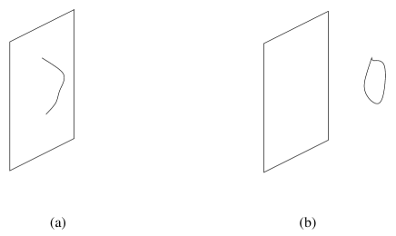
Figure 1: (a) open string description (b) closed string description

We are ready to discuss how the conversion “derives” AdS/CFT duality. AdS/CFT can be motivated by taking a viewpoint that there are two different but dual stringy descriptions of the same objects, D-branes. One description is via open strings with mixed Dirichlet and Neumann boundary conditions. In the other description one considers type IIB closed string theory expanded around the D-brane soliton solutions. Upon taking a low energy near horizon limit, the viewpoint leads, e.g., in the case of D3 branes, to the duality between ${\cal N}=4,D=4$ SYM theory and ${\cal N}=8,D=5$ gauged supergravity. To make the discussion slightly more general, consider a open string attached to an arbitrary odd dimensional brane. The open string propagates in the curved background produced by the presence of the brane. We start with a weakly coupled opens string theory in a pure open string formulation. and go to a strong coupling limit by S-duality. After the duality the appropriate degrees of freedom are a closed string in the same background. The closed string should be of type IIB and strongly coupled. In case of a D3 brane, the resulting closed string is in the D3 brane background, but can be considered as weakly coupled due to the SL(2,Z) self-duality [42]: the weakly coupled IIB closed string is connected by a chain of dualities to the starting point, a weakly coupled open string. In the low energy this leads to the duality between ${\cal N}=4$ SYM theory and IIB supergravity on AdS${}_{5}\times$S⁵. Similarly, starting with an open string in the background of D2/D4 branes we will get AdS/CFT conjecture concerning AdS${}_{4/7}\times$S^7/4.

One can give similar arguments for matrix theories. Consider an open superstring with the fermionic coordinates of opposite chiralities. Take fully Neumann boundary conditions. Apply the conversion procedure, i.e., one start with a very weak coupling and consider S-duality to go to a strong coupling limit. The closed string that appears will be of type IIA. In particular it will be strongly coupled. The strong coupling limit of IIA is M-theory [44]. On the other hand we can T-dualize the original open string to an open string with Dirichlet boundary conditions for the nine space dimensions. Therefore, one end of this operation is an open string with Dirichlet boundary conditions and the other end is M-theory. Once we go to a low energy limit, the two theories respectively reduce to quantum mechanics and eleven dimensional supergravity: we have the matrix theory conjecture of M-theory [45]. On the other hand, if we start with an opens string whose fermionic coordinates have the same chiralities, we will get IKKT matrix theory conjecture [46].

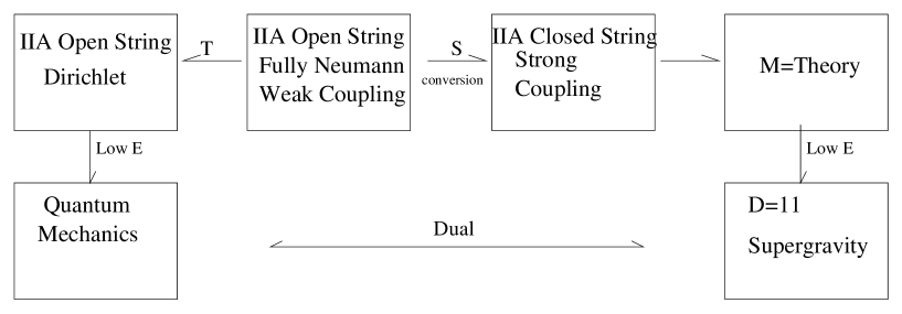
Figure 2: Duality chain for BFSS matrix theory

4 Conclusion

AdS/CFT conjecture was motivated in [5] by starting from an axiomatic assumption that there are two dual descriptions of D-branes, open and closed. We have argued here that the duality may originate from the conversion of an open strong into a closed string under a large coupling limit where the coupling constant approaches infinity. For that, we considered a (non-tachyonic) generalization of the analysis of [14] to a curved background with a constant $B$-field. Although we studied only a bosonic Born-Infeld action we believe that a similar analysis should be possible for a supersymmetric case, which is an interesting open problem. We noted that the duality under consideration implies, in low energy limits, very general dual relations between gauge theories and gravity theories. In particular it seems that AdS/CFT and matrix theory conjectures come from the same root, the conversion of an open string into a closed string under a strong coupling limit. It will be interesting to promote the discussions to a full string theory analysis.

Note Added: After this work was published, a paper [47] appeared which has partially related discussions.

Acknowledgements
For their valuable discussions I would like to thank B. Craps, N.S. Deger, A. Kaya, P. Kraus, F. Larsen, M. Roček, I. Rudychev, W. Siegel, T.A. Tran, A.A. Tseytlin, P. Yi and especially C.N. Pope. This work is supported by US Department of Energy under grant DE-FG03-95ER40917.

Appendix

In section 2 we imposed $g_{\circ i}=0$ for simplicity. Here we relax the condition. Since the calculations for the $B$-part remain the same we will not consider them. With $g_{\circ i}\neq 0$ the determinant can be rewritten as

$$-\mbox{Det}(g_{\mu\nu}+F_{\mu\nu})=-g_{\circ\circ}\mbox{Det}(h_{ik})-E^{{}^{(+)}}_{i}D^{ik}E^{{}^{(-)}}_{k}$$ (17)

where

$${E^{\pm}}_{i} = E_{i}\pm g_{\circ i}\;\;\;\;,\;\;\;\;h_{ij}=g_{ij}+F_{ij}$$

$$D^{ij}\;\; = (-1)^{i+j}\Delta^{ji}(h)\;\;\;,\;\;\;D=\mbox{Det}(h)\,h^{-1}$$ (18)

where $\Delta$ represents the minor matrix of $h$. The canonical momenta are

$$\pi^{i}=\frac{\tau}{\sqrt{-\mbox{Det}(g_{\mu\nu}+F_{\mu\nu})}}\;\frac{1}{2}(E^{{}^{(+)}}_{k}D^{ki}+D^{ki}E^{{}^{(-)}}_{k})$$ (19)

After some algebra one can show that

$${\cal H} = \frac{\tau}{\sqrt{-\mbox{Det}(g_{\mu\nu}+F_{\mu\nu})}}\left(-\mbox{Det}(h)g_{\circ\circ}+\frac{1}{2}g_{\circ i}\left(E^{{}^{(+)}}_{k}D^{ki}-D^{ik}E^{{}^{(-)}}_{k}\right)\right)$$ (20)

The Hamiltonian in terms of the canonical variables can be obtained by solving the following equation that it satisfies,

$${\cal H}^{2}-2g_{0l}u^{li}F_{ij}\pi^{j}\;{\cal H}+\frac{1}{G^{\circ\circ}}\left(\pi^{i}g_{ij}\pi^{j}\!+(F_{ij}\pi^{j})^{2}\right)=0$$ (21)

where $(\!F_{ij}\pi^{j})^{2}\equiv g^{ik}F_{ij}\pi^{j}F_{km}\pi^{m}$ and $\tau$ has been set to zero. We have also introduced, $u^{ij}$, the inverse matrix of $g_{ij}$. In general, $u^{ij}$ is not  the same as $g^{ij}$, the (ij)-th component of $g^{\mu\nu}$ although that was true in the case we considered in section two, i.e., in the case of $g_{i0}=0$. As before we perform a Legendre transformation with

$$K^{ij}=-\;\frac{\;g_{0l}u^{li}\pi^{j}-g_{0l}u^{lj}\pi^{i}+\frac{2}{G^{\circ\circ}}(F^{i}_{l}\pi^{l}\pi^{j}-F^{j}_{l}\pi^{l}\pi^{i})}{2{\cal H}-2g_{0l}u^{li}F_{ij}\pi^{j}}$$ (22)

where $F^{i}_{l}\equiv G^{ik}F_{kl}$. It is straightforward to show

$${\cal L}^{\prime}=-\frac{2}{G^{\circ\circ}}\;\frac{\pi^{i}g_{ij}\pi^{j}}{\;2{\cal H}-2g_{\circ l}u^{li}F_{ij}\pi^{j}}$$ (23)

Using the same definitions for the components of ${\cal K}^{\mu\nu}$, i.e.,

$${\cal K}^{\circ i}=-\pi^{i}\;\;\;,\;\;\;{\cal K}^{ij} = K^{ij}$$ (24)

One can show, after rather lengthy algebra, that

$$\frac{1}{2}{\cal K}^{\mu\nu}{\cal K}_{\mu\nu}=-\left(\frac{2}{G^{\circ\circ}}\right)^{2}\;\frac{(\pi^{i}g_{ij}\pi^{j})^{2}}{\;(2{\cal H}-2g_{\circ l}u^{li}F_{ij}\pi^{j})^{2}}$$ (25)

Therefore the dual Lagrangian has the same form as before,

$${\cal L}^{\prime}=\sqrt{-\frac{1}{2}{\cal K}^{{}^{\mu\nu}}{\cal K}_{{}_{\mu\nu}}}$$ (26)

and the discussions below equation (11) of section two remain the same.

References

- [1] J. Polchinski, Phys. Rev. Lett 75 (1995) 4724, hep-th/9510017
- [2] J. Maldacena, Adv. Theor. Math. Phys. 2 (1998) 231, hep-th/9711200
- [3] S.S. Gubser, I.R. Klebanov and A.M. Polyakov, Phys. Lett B428 (1998) 105, hep-th/9802109
- [4] E. Witten, Adv. Theor. Math. Phys. 2 (1998) 253, hep-th/9802150
- [5] I.Y. Park, Phys. Lett. B468 (1999) 213, hep-th/9907142
- [6] J. Khoury and H. Verlinde, Adv. Theor. Math. Phys. 3 (1999) 1893, hep-th/0001056
- [7] U.H. Danielsson, A. Guijosa, M. Kruczenski and B. Sundborg, JHEP 0005:028,2000, hep-th/0004187
- [8] M. Arnsdorf and L. Smolin, hep-th/0106073
- [9] A.A. Tseytlin, hep-th/9908105
- [10] G.W. Gibbons, hep-th/0106059
- [11] H.B. Nielsen and P. Olesen, Nucl. Phys. B57 (1973) 367
- [12] U. Lindstrom and R. von Unge, Phys. Lett. B403 (1997) 233, hep-th/9704051
- [13] U.Lindstrom and M. Zabzine, JHEP 0103 (2001) 014, hep-th/0101213
- [14] G.Gibbons, K. Hori and P. Yi, Nucl. Phys. B596 (2001) 136, hep-th/0009061
- [15] A.Sen, hep-th/0010240
- [16] M. Kleban, A. Lawrence and S. Shenker, hep-th/0012081
- [17] A.A Garasimov and S.L. Shatashvili, JHEP 0101,019 (2001), hep-th/0011009
- [18] B. Craps, P. Kraus and F. Larsen, hep-th/0105227
- [19] J.A. Harvey, D. Kutasov and E.J. Martinec, hep-th/0003101
- [20] D. Kutasov, M. Marino and G.Moore, JHEP 0100,045 (2000), hep-th/0009148
- [21] P. Yi, Nucl. Phys. B550 (1999) 214, hep-th/9901159
- [22] O. Bergman, K. Hori and P. Yi, Nucl. Phys. B580 (2000) 289, hep-th/0002223
- [23] G.W. Gibbons and K. Hashimoto, JHEP 0009 (2000) 013, hep-th/0007019
- [24] A.A. Tseytlin, Nucl. Phys. B469 (1996) 51, hep-th/9602064
- [25] J. Bagger and A. Galperin, Phys. Lett. B412 (1997) 296, hep-th/9707061
- [26] M. Rocek and A.A. Tseytlin, Phys. Rev. D59 (1999) 106001, hep-th/9811232
- [27] F. Gonzalez-Rey, I.Y. Park and M. Rocek, Nucl. Phys. B544 (1999) 243, hep-th/9811130
- [28] S. Bellucci, E. Ivanov and S. Krivonos, Phys. Lett. B460 (1999) 348, hep-th/9811244
- [29] P. Pasti, D. Sorokin and M. Tonin, Nucl. Phys. B591 (2000) 109, hep-th/0007048
- [30] P.S. Howe, O. Raetzel and E. Sezgin, JHEP 9808 , 011 (1998)
- [31] F. Gonzalez-Rey, B. Kulik, I.Y. Park and M. Rocek, Nucl. Phys. B544 (1999) 218, hep-th/9810152
- [32] N. Seiberg, L. Sussind and N. Toumbas, JHEP 0006:021,2000, hep-th/0005040
- [33] R. Gopakumar, J. Maldacena, S. Minwalla and A. Strominger, JHEP 0006:036,2000, hep-th/0005048
- [34] J.A. Shapiro and C.B. Thorn, Phys. Rev. D36 (1987) 432
- [35] M. Srednicki and R.P. Woodard, Nucl. Phys. B293 (1987) 612
- [36] M.B. Green and C.B. Thorn, Nucl. Phys. B367 (1991) 462
- [37] W. Siegel, Phys. Rev. D49 (1994) 4144
- [38] S. R. Das and S. P. Trivedi, Phys. Lett. B445 (1998) 142, hep-th/9804149
- [39] S. Ferrara, M.A. Lledo and A. Zaffaroni, Phys. Rev. D58 (1998) 105029, hep-th/9805082
- [40] I.Y. Park, A. Sadrzadeh and T.A. Tran, Phys. Lett. B497 (2001) 303, hep-th/0010116
- [41] S.R. Das and S.P. Trivedi, JHEP 0102, 046 (2001), hep-th/0011131
- [42] J.H. Schwarz, Phys. Lett. B360 (1995) 13, hep-th/9508143
- [43] S. Minwalla, JHEP 9810 002 (1998), hep-th/9803053
- [44] E. Witten, Nucl. Phys. B433 (1995) 85, hep-th/9503124
- [45] T. Banks, W. Fischler, S.H. Shenker and L. Susskind, Phys. Rev. D55 (1997) 5112, hep-th/9610043
- [46] N. Ishibashi, H. Kawai, Y. Kitazawa and A. Tsuchiya, Nucl. Phys. B498 (1997) 467, hep-th/9612115
- [47] H. Kawai and T. Kuroki, hep-th/0106103
- [48]