Quantized bulk fermions in the Randall-Sundrum brane model

Abstract

The lowest order quantum corrections to the effective action arising from quantized massive fermion fields in the Randall-Sundrum background spacetime are computed. The boundary conditions and their relation with gauge invariance are examined in detail. The possibility of Wilson loop symmetry breaking in brane models is also analyzed. The self-consistency requirements, previously considered in the case of a quantized bulk scalar field, are extended to include the contribution from massive fermions. It is shown that in this case it is possible to stabilize the radius of the extra dimensions but it is not possible to simultaneously solve the hierarchy problem, unless the brane tensions are dramatically fine tuned, supporting previous claims.

PACS number(s):11.10.Kk, 04.50.+h, 04.62.+v, 11.25.Mj
Keywords:Extra Dimensions, Brane Models, Quantum Fields.

I Introduction

The idea of extra dimensions was originally introduced in order to provide a unified description of the electromagnetic and gravitational interactions [1, 2] and further generalised to more than one extra dimension in order to allow the incorporation of non-abelian gauge fields [3]. More recent interest was generated in connection with supergravity and string theory [4, 5, 6].

In the past few years this idea is having a novel rejuvenation, particularly in relation with the resolution of the hierarchy problem. In addition, extra dimensions have also provided an interesting link between string theory and particle physics, motivating the construction of low energy effective theories with possible experimental signatures, and suggesting possible resolutions of many long standing problems of particle physics and cosmology.

This new perspective on higher dimensional theories was first pointed out in [7], where, in contrast to the standard belief that extra dimensions must be associated with extremely small length scales, it was noted that the extra dimensions could be as large as a millimeter, bringing the fundamental Planck scale closer to the electroweak scale and thus providing an explanation for the relative weakness of gravity with respect to the other forces. Unfortunately, this scenario with large extra dimensions suffers from an important drawback. It trades, in fact, a large ratio between the Planck scale and the electroweak scale for a large ratio between the compactification scale and the electroweak scale, not providing a satisfactory explanation to the hierarchy problem.

A brane model, with the interesting feature of having all the parameters of the theory of the same magnitude while still generating a very large hierarchy, was devised by Randall and Sundrum [8]. Their model is based on a 5-dimensional spacetime with the extra spatial dimension having an orbifold compactification. Two

3-branes with opposite tensions sit at the orbifold fixed points. The line element is

$$ds^{2}=e^{-2kr|\phi|}\eta_{\mu\nu}dx^{\mu}dx^{\nu}-r^{2}d\phi^{2}$$ (1)

with $x^{\mu}$ the usual 4-dimensional coordinates, $|\phi|\leq\pi$ with the points $(x^{\mu},\phi)$ and $(x^{\mu},-\phi)$ identified. of The 3-branes sit at $\phi=0$ and $\phi=\pi$. $k$ is a constant of the order of the Planck scale (the natural scale for the theory), and $r$ is an arbitrary constant associated with the size of the extra dimension. The interesting feature of the Randall-Sundrum model is that it can generate a TeV mass scale from the Planck scale in the higher dimensional theory. A field with a mass $m_{0}$ on the $\phi=\pi$ brane will have a physical mass of $m\simeq e^{-\pi kr}m_{0}$. By taking $kr\simeq 12$, and $m_{0}\simeq 10^{19}$ GeV, we end up with $m\simeq 1$ TeV.

Another interesting aspect of brane models is related to their field content. In the original version of the Randall-Sundrum model all of the standard model particles were confined on the brane, with only gravity moving throughout the bulk spacetime. Alternatives to confining particles on the brane have been investigated and a different number of reasons seem to suggest the necessity of new bulk physics [9, 10, 11, 12, 13, 14, 15, 16, 17, 18, 19].

Particularly relevant is the role of higher dimensional bulk fermions, primarily in relation with string theory, as they arise as superpartners of gravitational moduli and are inevitable in any string theory realisation of the brane world idea. In the context of particle physics phenomenology and string inspired model building some study has been devoted to include bulk fermions, but apart from a few exceptions, attention has been mostly concentrated on the massless case. However bulk fermion masses constitute an important feature which has to be taken into account for a different number of reasons.

In order to study possible phenomenological signatures, massless [16] and massive [17] bulk fermions have been considered. Interestingly, in [17] the resulting phenomenology is shown to be highly dependent on the value of the five dimensional fermion mass. In [12] a new way for obtaining small Dirac neutrino masses, without invoking a see-saw mechanism, was outlined. Within an effective field theory approach, massless chiral fermions and loop corrections to the effective action have been investigated [20, 21]. In [22] a comprehensive study of five dimensional brane models for neutrino physics has been presented.

Motivation for introducing massive bulk fermions also come from the need to localise fermion zero modes in the extra dimensions. In [24] a modification of the Dirac equation via a pseudo-scalar Yukawa coupling term of the form $m\chi(y)\bar{\Psi}\Psi$, with $\chi\propto\epsilon(y)$ and $\epsilon(y)$ the sign function, has been considered and it was shown that in this way it is possible to ensure both localisation and chirality. Non-chiral theories of fermions have been discussed in [23], where we stressed the fact that the fermion representations of the full Lorentz group in five dimensions have eight, rather than four, components.

The radius $r$ of the extra dimensions is assumed to be the vacuum expectation value of a scalar field, called the radion. In the scenario proposed by Randall and Sundrum, the radion has zero potential and consequently $r$ is not determined by the dynamics of the model. Therefore for this scenario to be physically acceptable, it is necessary to find a mechanism for generating such a potential which would stabilize the size of the extra dimensions.

Goldberger and Wise have suggested a solution to this problem [9]. They proposed the introduction of a bulk scalar field with appropriate interaction terms on the branes as a means to induce a stabilizing potential . Although this model provides a solution to the problem, it can be viewed as being very artificial and hence it is important to seek more natural alternatives.

The older Kaluza-Klein theories, based on factorisable geometries, homogeneous space) were affected by a similar difficulty. In that context, it was realised by Candelas and Weinberg that quantum effects from matter fields or gravity could be used to fix the size of the extra dimensions, stimulating the study of quantum effects in such scenarios [26, 27, 28, 29]. Analogously to that example it seems reasonable to investigate if the radius of the extra dimensions can be determined by quantum effects. Motivated by this analogy, the role of quantum effects has received some recent attention [30, 31, 32, 33, 23, 34, 35].

In [30] massless and conformally coupled fields obeying untwisted boundary conditions have been analysed. Massive scalar fields minimally coupled to the scalar curvature with untwisted boundary conditions have been considered in [31, 32]. In [33] massive scalar fields obeying twisted and untwisted boundary conditions with a non-minimal coupling have been investigated and a self-consistency relation has been obtained. In [33] the importance (in principle) for the inclusion of the induced gravity term has been pointed out and it has been computed in both the twisted and untwisted case. Massless fermion fields have been investigated in both [30] (for untwisted field configurations) and in [23] (for twisted as well as untwisted field configurations). Also in [23] it has been pointed out that the boundary condition structure it can be enlarged when considering a gauge symmetry. The main conclusion of [30, 31, 32, 33, 23] is that a severe fine tuning of the brane tensions is essential for the radius to be stabilized via quantum effects and the hierarchy problem to be solved simultaneously. The one-loop Casimir energy in five dimensional $S^{1}/{Z}_{2}$ and six dimensional $T^{2}/{Z}_{k}$ orbifolds has been considered in [34]. Some related work in M theory has been done in [35], where the Casimir energy is evaluated for a non-supersymmetric $E_{8}\times\bar{E}_{8}$ compactification of M theory on $S^{1}/{Z}_{2}$.

In the present paper we try to amplify the previous considerations and compute the radiative corrections to the effective action on a five dimensional classical background spacetime with an orbifold compactification including the contribution coming from massive Fermi fields. The next section is devoted to introducing the general framework and compute the one-loop vacuum energy for a single 4-component fermion. The relation between the boundary condition structure and gauge invariance is clarified in section 3 and the vacuum energy is computed for a fermion and scalar multiplet under general boundary conditions. The massless, conformally coupled case is discussed in section 4, as it provides a useful check on the method used. The possibility of Wilson loop symmetry breaking is deferred to section 5. In section 6 we discuss the self-consistency requirements in the model when quantum effects are included. Our conclusions are drawn in the last part of the paper.

II Effective Action

In this section we will evaluate the quantum corrections to a classical theory specified by a single massive bulk fermion on the Randall-Sundrum background spacetime. We follow the general method outlined in [31], which we will briefly review. It consists of first expanding the higher dimensional fields in terms of a complete set of modes and then integrating out the dependence on the extra dimension leaving an equivalent four dimensional theory with an infinite number of fields with masses quantized in some way:

$$S=\sum_{n}S_{n}~{}.$$ (2)

$S_{n}$ represents the dimensionally reduced theory for the $n^{th}-$mode, with differential operator given by ${\cal D}_{n}$. Having done this, the effective action is simply given by the sum over the modes:

$$\Gamma^{(1)}_{n}={1\over 2}\sum_{n}\ln det\left(\ell^{2}{\cal D}_{n}\right)~{}.$$ (3)

Since the one-loop effective action is expressed as the logarithm of the determinant of ${\cal D}_{n}$, it turns out to be advantageous to adopt a heat kernel method, namely writing the effective action in terms of a non-local kernel function $K_{n}(s,x,x^{\prime})$:

$$\Gamma^{(1)}=-{1\over 2}\sum_{n}\int d^{D}x|g|^{1/2}\int{ds\over s}TrK_{n}(s,x,x)~{},$$ (4)

where

$$-{\partial\over\partial s}K_{n}(s,x,x^{\prime})={\cal D}_{n}K_{n}(s,x,x^{\prime})~{},$$ (5)

$$K_{n}(0,x,x^{\prime})=\delta(x,x^{\prime})~{}.$$ (6)

It is now possible to use an asymptotic expansion for the heat kernel, in order to obtain an expansion in powers of the curvature:

$$K_{n}(s,x,x)\propto s^{-D/2}\sum_{k=0}^{\infty}(is)^{k}a_{k}(x)~{},$$ (7)

where the heat kernel coefficients $a_{k}(x)$ depend on geometrical invariants only.

The coefficients $a_{k}(x)$ are known for a wide class of differential operators defined on manifolds with and without boundaries with different types of boundary conditions (see [3, 36, 37, 38] and references therein), and recently the spectral geometry of operator of Laplace type on manifolds with singular surfaces has been considered also in connection with brane models [39, 40, 41].
The leading term, given by $a_{0}(x)$, represents the Casimir energy contribution to the cosmological constant. The next term is proportional to the four dimensional curvature and gives a gravity term induced by quantum effects. This term has received little attention in brane models, but it played a major role in the study of the self-consistency of the older Kaluza-Klein theories [42]. Additionally, the induced gravity term is essential if we wish to identify the physical value of the Newtonian gravitational constant in terms of the bare one. The next term in the expansion, proportional to $a_{3}(x)$, contains higher curvature terms and becomes important when considering higher derivative gravity models on brane backgrounds [43, 44, 45, 46, 47, 48, 49].

Strictly speaking, in the Randall-Sundrum scenario, where the 3-branes are flat, these terms are absent, however they make their appearance when curved branes are considered. In our analysis, we are simply after the vacuum energy and therefore these next-to-leading terms won’t be reported, although they are obtainable at ease with simple modifications of our calculation.

The result for the quantum corrections to the effective action is found to be divergent and needs to be regulated in some way. Here, following the procedure of [33], we choose to use dimensional regularisation.

A Kaluza-Klein reduction

The Kaluza-Klein reduction has been performed in a number of references (see for example [12]) and the details won’t be repeated here. Only in order to fix the notation and discuss few points of importance for the present work, we outline the essential steps. Initially, we consider a single chiral fermion on the spacetime described by (1) and whose action is given by

$$S=\int d^{4}x\int dy|g|^{1/2}\left(i\bar{\Psi}\underline{\gamma}^{M}D_{M}\Psi-m\cdot\epsilon(y)\bar{\Psi}\Psi\right)~{}.$$ (8)

For notational convenience, the coordinate $y$ describing the extra dimension is reparametrised by

$$y=r\phi~{},$$ (9)

The Kaluza-Klein reduction can be performed by decomposing the field $\Psi$ in its left and right components,

$$\Psi(x_{\mu},y)=\sum_{n}\left(\Psi_{R}^{(n)}(x_{\mu})g_{R}^{(n)}(y)+\Psi_{L}^{(n)}(x_{\mu})g_{L}^{(n)}(y)\right)$$ (10)

and then integrating over the extra dimension. This leaves us with

$$S=\sum_{n}\int d^{4}x\left(i\bar{\psi}_{n}\mbox{${\not{\hbox{\kern-2.0pt$\partial$}}}$}\psi_{n}-m_{n}\bar{\psi}_{n}\psi_{n}\right)~{},$$ (11)

where $\psi_{n}(x)=\Psi_{L}^{(n)}(x)+\Psi_{R}^{(n)}(x)$. The dependence of $\Psi$ on the extra dimension can be expressed as a combination of Bessel functions:

$$G_{L}^{(n)}(z_{n})=z_{n}^{1/2}\left(a^{(n)}_{L}J_{1/2+\nu}(z_{n})+b^{(n)}_{L}J_{-1/2-\nu}(z_{n})\right)~{},$$ (12)

$$G_{R}^{(n)}(z_{n})=z_{n}^{1/2}\left(a^{(n)}_{R}J_{1/2-\nu}(z_{n})+b^{(n)}_{R}J_{-1/2+\nu}(z_{n})\right)~{},$$ (13)

where $G_{(R,L)}^{(n)}=e^{-2k|y|}g_{(R,L)}^{(n)}$, $z_{n}=m_{n}e^{k|y|}/k$ and $\nu=m/k$.

The coefficients $a^{(n)}_{L}$, $b^{(n)}_{L}$, $a^{(n)}_{R}$, $b^{(n)}_{R}$ can be found by imposing some boundary conditions. The possible boundary conditions are related to the parity of the spinor field $\Psi$ under a chiral transformation. A possibility, which we will call $I$, is that the field $\Psi$ is even:

$$\gamma_{5}\Psi(x_{\mu},-y)=+\Psi(x_{\mu},y)~{},$$ (14)

implying that the mass eigenvalues are quantized according to the following transcendental equation:

$$J_{1/2+\nu}({m_{n}\over ka})J_{-1/2-\nu}({m_{n}\over k})-J_{1/2+\nu}({m_{n}\over k})J_{-1/2-\nu}({m_{n}\over ka})=0~{},$$ (15)

where $a=e^{-kr\pi}$. The other possibility, which we will call $II$, is given by:

$$\gamma_{5}\Psi(x_{\mu},-y)=-\Psi(x_{\mu},y)~{},$$ (16)

leading to

$$J_{-1/2+\nu}({m_{n}\over ka})J_{1/2-\nu}({m_{n}\over k})-J_{-1/2+\nu}({m_{n}\over k})J_{1/2-\nu}({m_{n}\over ka})=0~{}.$$ (17)

It is worth commenting a bit further on the two types of parity conditions, and the mass term chosen in (8). Generally we would expect that because of the ${Z}_{2}$ identification of the extra dimension, we could have

$$\Psi(x,-y)=B\Psi(x,y)$$ (18)

for some matrix $B$. The requirements that the action, or Hamiltonian, remain invariant under the ${Z}_{2}$ identification place certain constraints on $B$, which are easily shown to be

$$B^{\dagger}B=I$$ (19)

$$[\gamma^{0}\gamma^{i},B]=0,~{}\mbox{$i=1,~{}2,~{}3$}$$ (20)

$$\{\gamma^{0}\gamma_{5},B\}=0$$ (21)

where $\{,\}$ is the anticommutator. The only way to solve these relations occurs if

$$B=e^{i\delta}\gamma_{5}$$ (22)

for some arbitrary phase factor $\delta$. Finally we use the fact that $B$ as defined in (18) must provide a representation of the group ${Z}_{2}$, which requires

$$B^{2}=I~{}.$$ (23)

(This is just a fancy way of saying that two reflections gives us back the identity.) This fixes $\delta$ to be $0$ or $\pi$, and hence

$$B=\pm\gamma_{5}$$ (24)

are the only two possibilities.

Regarding the mass term, the identification of $y$ with $-y$ on the fields with $B=\pm\gamma_{5}$ does not leave the mass term invariant if $m$ is a constant. Choosing $m\propto\epsilon(y)$ is the simplest possibility for an invariant mass term. (A constant mass term can be used with eight component spinor representations [23]).

B Evaluation of the vacuum energy

We want to compute the vacuum energy for the theory described by the action (11). The fact that type $I$ and type $II$ boundary conditions differ only for the order of the Bessel functions simplifies the subsequent analysis and allows to deal with both cases at once. In what follows we define

$$\mu=1/2+\nu,\mbox{for type $I$ boundary conditions}$$ (25)

and

$$\mu=1/2-\nu,\mbox{for type $II$ boundary conditions}~{}.$$ (26)

Following [33], we use the form for the heat kernel described in [50]. After some well known manipulation the one-loop effective action can be expressed as

$$\Gamma^{(1)}=-{i\over 2}\sum\ln det\left(\ell^{2}(\Box+{1\over 4}R+m_{n}^{2})\right)~{}.$$ (27)

Now using the heat kernel expansion for the previous operator we have:

$$\Gamma^{(1)}=\int d^{4}x|g|^{1/2}{\cal L}_{\Lambda}^{F}~{},$$ (28)

with

$${\cal L}_{\Lambda}^{F}=-{1\over 2}(4\pi)^{-2}\lim_{D\rightarrow 4}\Gamma(-D/2)\sum_{n}m_{n}^{D}~{}.$$ (29)

The masses $m_{n}$ are quantized according to the following eigenvalue equation:

$$P_{\mu}(x_{n})=J_{\mu}(x_{n})J_{-\mu}(ax_{n})-J_{\mu}(ax_{n})J_{-\mu}(x_{n})=0~{},$$ (30)

where, for convenience, we have defined

$$m_{n}=kax_{n}~{}.$$ (31)

Introducing $\epsilon=D-4$, we find

$${\cal L}_{\Lambda}^{F}=-{1\over 32\pi^{2}}\lim_{\epsilon\rightarrow 0}(ka)^{4+\epsilon}v(\epsilon)~{},$$ (32)

where

$$v(\epsilon)=\Gamma(-2-\epsilon/2)\sum_{n}x_{n}^{4+\epsilon}~{}.$$ (33)

The method we use to compute the previous sum is a simple modification of the technique developed in [51, 52], which allows to evaluate the $\zeta-$function using only the basic properties of the eigenvalue equation.

A simple application of the residue theorem permits to convert the previous sum into a contour integral:

$$v(\epsilon)=\frac{\Gamma(-2-{\epsilon\over 2})}{2\pi i}\oint_{\mathcal{C}}dz\,z^{4+\epsilon}\,\frac{d}{dz}\ln\,P_{\nu}(z)\;,$$ (34)

where ${\mathcal{C}}$ is any contour which encloses the positive zeros of $P_{\nu}(z)$. After some manipulations, with an appropriate choice for the contour ${\mathcal{C}}$, $v(\epsilon)$ can be recast in the following form:

$$v(\epsilon)={1\over\Gamma(3+\epsilon/2)}\int_{0}^{\infty}dyy^{4+\epsilon}{d\over dy}\ln Q_{\mu}(y)~{},$$ (35)

with

$$Q_{\mu}(y)=I_{\mu}(y)K_{\mu}(ay)-I_{\mu}(ay)K_{\mu}(y)~{}.$$ (36)

Expression (35) can be rearranged in order to isolate the divergent contributions and exploiting the dependence on $a$. The analytical continuation of (35) to $\Re(\epsilon)>2$ can be carried out noting that the impediment to the convergence of (35) comes from the behaviour of $Q_{\mu}(z)$ at large $z$. Analogously to the scalar field case, we will define

$$I_{\nu}(z)=\frac{e^{z}}{\sqrt{2\pi z}}\,\Sigma^{(I)}(z)\;,$$ (37)

$$K_{\nu}(z)=\sqrt{\frac{\pi}{2z}}\,e^{-z}\,\Sigma^{(K)}(z)\;.$$ (38)

For large $z$ the asymptotic expansions for the Bessel functions show that

$$\Sigma^{(I)}(z)\simeq\sum_{k=0}^{\infty}\alpha_{k}\,z^{-k}\;,$$ (39)

where

$$\alpha_{k}=\frac{(-1)^{k}\,\Gamma(\nu+k+\frac{1}{2})}{2^{k}\,k!\,\Gamma(\nu-k+\frac{1}{2})}\;,$$ (40)

and

$$\Sigma^{(K)}(z)\simeq\Sigma^{(I)}(-z)\;.$$ (41)

With these positions, after some manipulations of (35), we end with

$$v(\epsilon)=J(a)+A+a^{-4-\epsilon}B-{4d_{4}\over\epsilon\Gamma(3+\epsilon/2)}(1+a^{-4-\epsilon})~{},$$ (42)

where

$$J(a)={1\over\Gamma(3+\epsilon/2)}\int_{0}^{\infty}dyy^{4+\epsilon}{d\over dy}\ln~{}\left(1-{K_{\mu}(y)I_{\mu}(ay)\over K_{\mu}(ay)I_{\mu}(y)}\right)~{},$$ (43)

$$A={1\over\Gamma(3+\epsilon/2)}\left\{\int_{1}^{\infty}dyy^{4+\epsilon}{d\over dy}\left(\ln\Sigma^{(I)}(y)-\sum_{n=1}^{N}d_{n}y^{-n}\right)\right.$$

$$+\int_{1}^{\infty}dyy^{4+\epsilon}{d\over dy}\left(\sum_{n=1,n\neq 4}^{N}d_{n}y^{-n}\right)+$$

$$\left.+\int_{0}^{1}dyy^{4+\epsilon}{d\over dy}\ln I_{\mu}(y)+\int_{1}^{\infty}dyy^{4+\epsilon}{d\over dy}\ln{e^{z}\over\sqrt{2\pi z}}\right\}~{},$$ (44)

$$B={1\over\Gamma(3+\epsilon/2)}\left\{\int_{1}^{\infty}dyy^{4+\epsilon}{d\over dy}\left(\ln\Sigma^{(K)}(y)-\sum_{n=1}^{N}(-1)^{-n}d_{n}y^{-n}\right)+\right.$$

$$+\int_{1}^{\infty}dyy^{4+\epsilon}{d\over dy}\left(\sum_{n=1,n\neq 4}^{N}(-1)^{-n}d_{n}y^{-n}\right)+$$

$$\left.+\int_{0}^{1}dyy^{4+\epsilon}{d\over dy}\ln K_{\mu}(y)+\int_{1}^{\infty}dyy^{4+\epsilon}{d\over dy}\ln\left(e^{-z}\sqrt{{\pi\over 2z}}\right)\right\}~{}.$$ (45)

The coefficients $d_{n}$, which determine the pole structure of the vacuum energy are given by the large-$z$ behaviour of $\Sigma^{(I)}(z)$:

$$\ln\,\Sigma^{(I)}(z)\simeq\sum_{k=1}^{\infty}d_{k}\,z^{-k}~{},$$ (46)

and are immediately evaluated using a Taylor expansion.

The unrenormalized one-loop vacuum energy can, finally, be written as

$${\cal L}_{\Lambda}^{F}=-{(ka)^{4}\over 64\pi^{2}}\int_{0}^{\infty}dyy^{4}{d\over dy}\ln~{}\left\{1-{K_{\mu}(y)I_{\mu}(ay)\over K_{\mu}(ay)I_{\mu}(y)}\right\}-$$

$$-{(ka)^{4+\epsilon}\over 32\pi^{2}}\left(A+a^{-4-\epsilon}B-{4d_{4}\over\epsilon\Gamma(3+\epsilon/2)}(1+a^{-4-\epsilon})\right)~{}.$$ (47)

The previous expression is found to be divergent and needs to be renormalized. The renormalization can be performed by using the brane tensions. In a previous work [33] we have found that when pushing the heat kernel expansion to higher orders there is the need to augment the brane tension with terms proportional to powers of the curvature in order to remove the pole terms. The same happens in the fermion case. However, in this calculation we truncated the expansion to first order and we don’t need to consider this possibility. Proceeding as in the scalar case, one can write the brane sector of the action as

$$S_{brane}=-\int d^{4}x|g|^{1/2}\left\{V_{h}+a^{4}V_{v}\right\}~{},$$ (48)

and express the bare quantities in terms of the renormalized ones:

$$V_{v,h}=V_{v,h}^{R}+\delta V_{v,h}~{},$$ (49)

where

$$\delta V_{v,h}={\delta V_{v,h}^{-1}\over\epsilon}+\delta V_{v,h}^{0}~{},$$ (50)

with $\delta V_{v,h}^{-1}$ and $\delta V_{v,h}^{0}$ independent of $\epsilon$. By using (47), (49), (50) the renormalization is straightforward leading to the following counterterms:

$$\delta V_{h}^{-1}=\delta V_{v}^{-1}={k^{4}\over 16\pi^{2}}d_{4}~{},$$ (51)

$$\delta V_{h}^{0}=-{k^{4}\over 32\pi^{2}}B~{},$$ (52)

$$\delta V_{v}^{0}=-{k^{4}\over 32\pi^{2}}A~{}.$$ (53)

In performing finite renormalizations, the $a$ dependence of the effective action has been crucial. In fact, all the terms in ${\cal L}_{\Lambda}^{F}$, except for $J(a)$, have the same functional dependence of the brane part of the action. Using the freedom to perform finite renormalizations we have absorbed in the counterterms everything apart from $J(a)$. This leaves the following expression for the renormalized vacuum energy:

$${\cal L}_{\Lambda}^{F}=-V_{h}^{R}-a^{4}V_{v}^{R}+{(ka)^{4}\over 16\pi^{2}}\int_{0}^{\infty}dyy^{3}\,\ln~{}\left\{1-{K_{\mu}(y)I_{\mu}(ay)\over K_{\mu}(ay)I_{\mu}(y)}\right\}~{}.$$ (54)

The result is plotted in figure (1). It qualitatively resembles the result for massless fermions given by Garriga at al. [30]. Note that replacing $\mu$ by $-\mu$ leaves the result unchanged appart from a shift in $V_{v}^{R}$, and therefore results with type $II$ boundary conditions with mass $m$ are equivalent to results for type $I$ boundary conditions with mass $m-k$.

III Gauge symmetry and boundary conditions

In the following we extend the previous considerations in order to discuss the most general boundary conditions consistent with the orbifold symmetry and the homogeneity of the spacetime. The interplay between gauge invariance and boundary conditions is also investigated. Once the boundary conditions are specified, the vacuum energy for a fermion and scalar multiplet, described by

$$S=S_{S}+S_{F}~{},$$ (55)

where

$$S_{S}={1\over 2}\int d^{4}xdy|g|^{1\over 2}\left\{g^{\mu\nu}\partial_{\mu}\Phi_{I}^{*}\partial_{\nu}\Phi_{I}-m_{S}^{2}\Phi^{*}_{I}\Phi_{I}-\xi R^{2}\Phi^{*}_{I}\Phi_{I}\right\}~{},$$ (56)

$$S_{F}=\int d^{4}xdy|g|^{1\over 2}\left\{i\bar{\Psi}_{I}\underline{\gamma}^{M}D_{M}\Psi_{I}-m_{F}~{}\epsilon(y)\bar{\Psi}_{I}\Psi_{I}\right\}~{},$$ (57)

is computed for a variety of boundary conditions. We use the label $I$ to index the field multiplets.

A Homogeneous boundary conditions

It was pointed out many years ago that the boundary conditions of a quantum field become very rich as soon as the spacetime upon which it is based has a non-trivial topological structure [53, 54]. Specifically, if the spacetime is multiply connected, the fields need not be single valued, being, in fact, required to obey weaker boundary conditions. It was also noted that the homogeneity of the spacetime and gauge symmetries produced non trivial constraints on the boundary structure of the fields.

A similar situation occurs in the Randall-Sundrum model, where the boundary conditions can be altered from the ones considered in the previous section, according to the symmetries of the action.

The boundary conditions have to be specified in order to relate the fields at identified points along the extra dimension and since they have to ensure that the action is single valued, we have the freedom to impose weaker boundary conditions on the fields. We assume that the manifold upon which the quantum field theory is homogeneous, meaning that that the physics is the same at every point.

The most general boundary conditions we can write are

$$\Phi_{I}(x_{\mu},-y)=\Sigma_{IJ}^{b}\Phi_{J}(x_{\mu},y)~{},$$ (58)

$$\Psi_{I}^{\sigma}(x_{\mu},-y)=\Delta_{IJ}^{b}\Lambda^{\sigma\rho}_{b}\Psi_{J}^{\rho}(x_{\mu},y)~{}.$$ (59)

$b=v,~{}h$, means that we can have different boundary conditions at the two branes. $\Sigma$ and $\Delta$ are global gauge transformations and $\Delta^{2}=1$, $\Sigma^{2}=1$. The requirement that the action is invariant under (58), (59) results in the following conditions:

$$\Delta_{IJ}^{b*}\Delta_{JK}^{b}=\delta_{IK}~{},$$ (60)

$$\Lambda^{\dagger}\gamma^{0}\gamma^{\mu}\Lambda=\gamma^{0}\gamma^{\mu}~{},$$ (61)

$$\Lambda^{\dagger}\gamma^{0}\Lambda=-\gamma^{0}~{},$$ (62)

$$\Sigma_{IJ}^{b*}\Sigma_{JK}^{b}=\delta_{IK}~{}.$$ (63)

Relations (61), (62) are satisfied uniquely by choosing

$$\Lambda=\pm\gamma^{5}~{}.$$ (64)

These are a generalization of the results for $B$ we wrote down earlier. The boundary conditions can be further constrained when taking into account the gauge symmetries of the theory. If the theory is gauge invariant, it would be expected that fields in the same gauge equivalence class satisfy the same boundary conditions, which, in other words, means that boundary conditions should be preserved under a gauge transformation. To exploit this, insert at each brane a gauge transformation $U\in G$, where $G$ is the gauge group:

$$\Phi_{I}^{\prime}(x_{\mu},y)=U_{S}^{b}(x_{\mu},y)\Phi_{I}(x_{\mu},y)~{},$$ (65)

$$\Psi_{I}^{\prime}(x_{\mu},y)=U_{F}^{b}(x_{\mu},y)\Psi_{I}(x_{\mu},y)~{}.$$ (66)

Requiring that the primed fields satisfy the same boundary conditions as the unprimed fields together with the requirement that the gauge transformation be single-valued gives:

$$[U^{b}_{S}(x_{\mu},y),\Sigma^{b}]=0~{},$$ (67)

$$[U^{b}_{F}(x_{\mu},y),\Delta^{b}]=0~{}.$$ (68)

Relations (67), (68) represent the symmetries of the boundary conditions [54].

Some comments are now in order. We have seen that the boundary conditions the fields are required to obey are weaker the larger is the symmetry of the theory and are constrained by the gauge invariance and ${Z}_{2}-$symmetry of the action. Among these constraints are the commutation relations given above. These commutation relations cannot be satisfied for any choice of the matrices $\Delta$ and $\Sigma$, meaning that if we want to keep the boundary conditions general, we have to restrict the original symmetry of the theory, which in turn means breaking the gauge symmetry at classical level. If we want to maintain the original symmetry of the classical theory, we are forced to restrict the matrices $\Delta$ and $\Sigma$ in order to satisfy the constraints found, i.e. they must belong to the center of the gauge group $G$.

It is instructive to see how this work in simple cases. If we consider a single scalar field, relation (63) implies that $\Sigma=\pm 1$ (the commutation relations are trivially satisfied in this case). This gives:

$$\phi(x_{\mu},-y)=\pm\phi(x_{\mu},y)~{},$$ (69)

where the $+$ sign gives the untwisted field configuration considered in [30, 31, 32, 33, 23], and the $-$ sign gives the twisted configuration considered in [33, 23]. In the single fermion case $\Lambda=\pm\gamma^{5}$ and $\Delta=e^{i\theta}$. The boundary conditions are then

$$\Psi(x_{\mu},-y)=\pm e^{i\theta}\Psi(x_{\mu},y)~{},$$ (70)

and the condition $\Delta^{2}=1$ implies $\theta=0$, which gives the fields configurations considered in the previous section.

B Effective action

In this section we will evaluate the effective action for situations in which a richer boundary structure is possible.

A first simple choice is to take a single real scalar field obeying different boundary conditions at the two branes. Two possibilities arise: the field is even at $y=0$ and odd at $y=\pi r$ or viceversa. We call these two cases ‘twisted’ and label them $T_{I}$ and $T_{II}$ respectively. The boundary conditions can be applied in a straighforward manner giving for the eigenvalue equation (the functions $j_{\nu},~{}y_{\nu},~{}i_{\nu},~{}k_{\nu}$ in the scalar case are the ones defined in [33]):

$$j_{\nu}(ax_{n})Y_{\nu}(x_{n})-y_{\nu}(ax_{n})J_{\nu}(x_{n})=0~{},$$ (71)

for type $T_{I}$ and

$$j_{\nu}(x_{n})Y_{\nu}(ax_{n})-y_{\nu}(x_{n})J_{\nu}(ax_{n})=0~{},$$ (72)

for type $T_{II}$. The computation of the vacuum energy is no different from the previous case and the renormalized quantum corrections can be written as

$${\cal L}_{\Lambda}^{S}={(ka)^{4}\over 64\pi^{2}}\int dyy^{4}g_{\nu}^{(T_{I},~{}T_{II})}(y)~{},$$ (73)

where

$$g_{\nu}^{T_{I}}(y)=1-{i_{\nu}(ay)K_{\nu}(y)\over k_{\nu}(ay)I_{\nu}(y)}~{},$$ (74)

and

$$g_{\nu}^{T_{II}}(y)=1-{k_{\nu}(y)I_{\nu}(ay)\over i_{\nu}(y)K_{\nu}(ay)}~{}.$$ (75)

Another simple possibility is to consider a single fermion field obeying different boundary conditions at the two branes. There are two possibilities:

$$\Psi(x_{\mu},-y)=+\gamma^{5}\Psi(x_{\mu},y)~{}~{}~{}~{}\mbox{at $y=0$}~{},$$ (76)

$$\Psi(x_{\mu},-y)=-\gamma^{5}\Psi(x_{\mu},y)~{}~{}~{}~{}\mbox{at $y=\pi r$}~{},$$ (77)

and the reversed one:

$$\Psi(x_{\mu},-y)=-\gamma^{5}\Psi(x_{\mu},y)~{}~{}~{}~{}\mbox{at $y=0$}~{},$$ (78)

$$\Psi(x_{\mu},-y)=+\gamma^{5}\Psi(x_{\mu},y)~{}~{}~{}~{}\mbox{at $y=\pi r$}~{}.$$ (79)

The mass eigenvalue equation is

$$J_{-\mu}(ax_{n})j_{\mu}(x_{n})-J_{\mu}(ax_{n})j_{-\mu}(x_{n})=0~{},$$ (80)

with $\mu=1/2+\nu$ for the first case and $\mu=\nu-1/2$ for the second case. For convenience, we have defined

$$j_{\mu}(z)=\left({1\over 2}-\nu\right)J_{\mu}(z)+zJ_{\mu}^{\prime}(z)~{},$$ (81)

$$k_{\mu}(z)=\left({1\over 2}-\nu\right)K_{\mu}(z)+zK_{\mu}^{\prime}(z)~{}.$$ (82)

The evaluation of the vacuum energy goes along the same lines as before and the renormalized contribution is found to be:

$${\cal L}_{\Lambda}^{F}={(ka)^{4}\over 16\pi^{2}}\int_{0}^{\infty}dyy^{3}\,ln~{}\left\{1-{k_{\mu}(y)I_{\mu}(ay)\over K_{\mu}(ay)i_{\mu}(y)}\right\}~{}.$$ (83)

The problem of computing the radiative corrections becomes more complicated, when a gauge symmetry is considered, due to the enlarged complexity of the boundary conditions. We have seen that, in order to maintain the gauge symmetry at classical level, the boundary conditions have to satisfy certain symmetries, specifically $\Delta$ and $\Sigma$ have to belong to the center of the gauge group $G$.

As an example, let us consider $G=SU(N)$. $\Delta$ belongs to the center of $SU(N)$. This modifies the boundary conditions in a simple way: the boundary conditions that each fermion component has to obey can be of type $I$, $II$, $T_{I}$ or $T_{II}$. This can be incorporated in the evaluation of the vacuum energy in a straightforward manner, giving:

$${\cal L}_{\Lambda}^{F}=\sum_{\kappa\in{(I,~{}II,~{}T_{I},~{}T_{II})}}N_{\kappa}^{F}{\cal L}_{\Lambda}^{F}(\kappa)~{},$$ (84)

where $N_{\kappa}^{F}$ represents the number of components satisfying type $\kappa$ boundary conditions and ${\cal L}_{\Lambda}^{F}(\kappa)$ is the vacuum energy for each component obeying type $\kappa$ boundary conditions.

Another simple example is to consider an $SO(N)$ scalar theory, for which the situation is similar to the previous one, giving:

$${\cal L}_{\Lambda}^{S}=\sum_{\kappa\in{(I,~{}II,~{}T_{I},~{}T_{II})}}N_{\kappa}^{S}{\cal L}_{\Lambda}^{S}(\kappa)~{},$$ (85)

where $N_{\kappa}^{S}$ represents the number of scalar components satisfying type $\kappa$ boundary conditions and ${\cal L}_{\Lambda}^{S}(\kappa)$ is the vacuum energy for each component obeying type $\kappa$ boundary conditions.

All this can be generalised to a general gauge group whose center is trivial. In this case the boundary conditions scalar and fermion fields ought to satisfy are still of the same type as before, giving:

$${\cal L}_{\Lambda}={\cal L}_{\Lambda}^{S}+{\cal L}_{\Lambda}^{F}=\sum_{\kappa\in{(I,~{}II,~{}T_{I},~{}T_{II})}}\left\{N_{\kappa}^{F}{\cal L}_{\Lambda}^{F}(\kappa)+N_{\kappa}^{S}{\cal L}_{\Lambda}^{S}(\kappa)\right\}~{}.$$ (86)

IV Conformally coupled case

The massless, conformally coupled case (studied in [30] for untwisted field configurations and in [23] for both the twisted and untwisted case) is worth of some special attention and provides a useful check on the general method used in the previous sections.

For type $I$ and type $II$ boundary conditions $\mu=1/2$, (43) can be expressed in terms of elementary functions and the integrals are now evaluated at ease, giving for the renormalized one-loop vacuum energy:

$${\cal L}_{\Lambda}^{F}=-{3k^{4}a^{4}\over 128\pi^{2}}\zeta(5)(1-a)^{-4}~{}.$$ (87)

Similarly, for type $T_{I}$ and $T_{II}$ boundary conditions $\mu=1/2$ and a straightforward calculation of (73) leads to

$${\cal L}_{\Lambda}^{F}={15\over 16}{3\over 128\pi^{2}}{k^{4}a^{4}\over(1-a)^{4}}\zeta(5)~{}.$$ (88)

The previous results can be also dealt with by direct summation of the mass eigenvalues $m_{n}$, which are, in general, given by

$$m_{n}={ka\over 1-a}(n\pi\pm\theta)~{},$$ (89)

where $\theta=0$ gives the untwisted field configuration, and $\theta={\pi\over 2}$ gives twisted one. The sum over the modes in ${\cal L}_{\Lambda}^{F}$ can be performed by using the properties of the $\zeta-$function and without the need of any renormalization:

$${\cal L}_{\Lambda}^{F}=-\lim_{D\rightarrow 4}{1\over 32\pi^{2}}{(\pi ka)^{D}\over(1-a)^{D}}\Gamma(-D/2)\left(\sum_{n=1}^{\infty}(n+\theta)^{D}+\sum_{n=1}^{\infty}(n-\theta)^{D}\right)~{}.$$ (90)

The previous result can be expressed in terms of the Hurwitz $\zeta-$ function:

$${\cal L}_{\Lambda}^{F}=-\lim_{D\rightarrow 4}{1\over 32\pi^{2}}{(\pi ka)^{D}\over(1-a)^{D}}\Gamma(-D/2)\left(\zeta_{H}(-D,\theta)+\zeta_{H}(-D,1-\theta)\right)~{},$$ (91)

which, by using basic properties of $\zeta_{H}$, can be recast in the form

$${\cal L}_{\Lambda}^{F}=-{3\over 128\pi^{2}}{(ka)^{4}\over(1-a)^{4}}\sum{\cos 2n\theta\over n^{5}}~{}.$$ (92)

Immediate inspection of (92) reproduces (87) for $\theta=0$ and (88) for $\theta=\pi/2$, as it must be.

V Topological symmetry breaking

An interesting feature of the boundary conditions on the branes is the possibility of breaking bulk gauge symmetries. The residual symmetries are those which commute with the two matrices $\Sigma^{h}$ and $\Sigma^{v}$ introduced in section 3.1. The symmetry breaking mechanism is similar to the Wilson-loop symmetry breaking mechanism in non-simply connected spacetimes [53, 54, 55, 56, 57, 58].

There are two equivalent ways to describe this type of symmetry breaking. The non-trivial boundary conditions are useful for evaluating and comparing the effective action for different symmetry breaking schemes, as we shall do below. Alternatively, it is possible to simplify the boundary conditions by performing a gauge transformation which introduces a pure gauge field stretching between the two branes. This ‘Wilson line’ is the analog of the Wilson loop in the Wilson loop mechanism. If the field strength vanishes, the line integral of the gauge field along a loop is conserved. This need not be true for the Wilson line and the symmetry breaking becomes associated with a set of moduli fields.

We shall concentrate on the possible symmetry breaking schemes fields with an $SU(N)$ gauge symmetry. The matrices $\Sigma^{h}$ and $\Sigma^{v}$ satisfy $(\Sigma^{h})^{2}=(\Sigma^{v})^{2}=I$, the unit matrix. By considering the eigenspaces of $[\Sigma^{h},\Sigma^{v}]^{2}$, it is easy to show that there is a basis in which the matrices take the block-diagonal form

$$\Sigma^{h} = {\rm diag}\{\pm 1,\dots,\mp 1,\sigma_{3},\dots,\sigma_{3}\}~{},$$ (93)

$$\Sigma^{v} = {\rm diag}\{\pm 1,\dots,\pm 1,\sigma_{\theta_{1}},\dots,\sigma_{\theta_{n}}\}~{},$$ (94)

where $\sigma_{1}$, $\sigma_{2}$, $\sigma_{3}$ are the Pauli matrices and

$$\sigma_{\theta}=\sigma_{3}\cos 2\theta+\sigma_{1}\sin 2\theta~{}.$$ (95)

The residual symmetry group is then

$$SU(n_{1})\times SU(n_{2})\dots\times SU(n_{p})\times U(1)^{q}.$$ (96)

There are $SU(n)$ factors for each of the four combinations of the $\pm 1$ entries along the diagonals of the matrices and further $SU(n)$ factors for each repeated value of $\theta$.

For example, if $G$ is the group $SU(5)$, we can take

$$\Sigma^{h} = {\rm diag}\{-1,-1,-1,\sigma_{3}\}~{},$$ (97)

$$\Sigma^{v} = {\rm diag}\{-1,-1,-1,\sigma_{\theta}\}~{}.$$ (98)

The group reduces to $G\to SU(4)\times U(1)$ if $\theta=0$ or $\pi/2$ and $G\to SU(3)\times U(1)$ otherwise.

The action (56) or (57) splits into separate terms, with one term for each of the block diagonal entries (94). Each term gives a contribution to the effective potential. The $\pm 1$ entries correspond to the type $I$ and $II$, twisted and untwisted boundary conditions considered in section 3.2. The $\sigma_{\theta}$ entries correspond to the following boundary conditions on the fermion modes at the hidden brane $y=0$ and the visible brane $y=r\pi$,

$$G_{R}(0) = \sigma_{3}G_{R}(0)~{},$$ (99)

$$G_{R}^{\prime}(0) = -\sigma_{3}G_{R}^{\prime}(0)~{},$$ (100)

$$G_{R}(r\pi) = \sigma_{\theta}G_{R}(r\pi)~{},$$ (101)

$$G_{R}^{\prime}(r\pi) = -\sigma_{\theta}G_{R}^{\prime}(r\pi)~{}.$$ (102)

The boundary conditions for $G_{L}$ modes and scalar field modes have an equivalent form.

The fermion mode functions were given in equations (12) and (13). Substituting these modes into the boundary conditions gives the values for the masses $m_{n}$. Introduce

$$p_{\nu} = J_{\nu}\left({m_{n}\over k}\right)Y_{\nu}\left({m_{n}\over ka}\right)-J_{\nu}\left({m_{n}\over ka}\right)Y_{\nu}\left({m_{n}\over k}\right)~{},$$ (103)

$$q_{\nu} = J_{\nu}\left({m_{n}\over k}\right)Y^{\prime}_{\nu}\left({m_{n}\over ka}\right)-J_{\nu}\left({m_{n}\over ka}\right)Y^{\prime}_{\nu}\left({m_{n}\over k}\right)~{},$$ (104)

$$r_{\nu} = J^{\prime}_{\nu}\left({m_{n}\over k}\right)Y_{\nu}\left({m_{n}\over ka}\right)-J^{\prime}_{\nu}\left({m_{n}\over ka}\right)Y_{\nu}\left({m_{n}\over k}\right)~{},$$ (105)

$$s_{\nu} = J^{\prime}_{\nu}\left({m_{n}\over k}\right)Y^{\prime}_{\nu}\left({m_{n}\over ka}\right)-J^{\prime}_{\nu}\left({m_{n}\over ka}\right)Y^{\prime}_{\nu}\left({m_{n}\over k}\right).$$ (106)

The values of $m_{n}$ are given by

$$p_{\nu+1/2}s_{\nu+1/2}\cos^{2}\theta+q_{\nu+1/2}r_{\nu+1/2}\sin^{2}\theta=0.$$ (107)

For $\theta=0$, this reduces to the previous cases $p_{\nu+1/2}=0$ (for type $I$ boundary conditions) and $s_{\nu+1/2}=0$ (for type $II$ boundary conditions).

In the massless fermion and the conformally invariant scalar field theories the Bessel functions become trigonometric functions and the values of $m_{n}$ are given by (89). The vacuum energy from one $\theta$ ‘block’ can be expressed in terms of Hurwitz zeta functions and evaluates to

$${\cal L}_{V}=\pm{3gk^{4}a^{4}\over 128\pi^{2}}(1-a)^{-4}\sum_{n=1}^{\infty}{\cos(2n\theta)\over n^{5}}$$ (108)

where the upper sign is for fermions, the lower for bosons and $g$ is the dimension of the fermion representation. The vacuum energy is extremised for $\theta=0$ and $\theta=\pi/2$, where the result reduces to the untwisted and twisted results respectively. This remains the case for massive fields because of the symmetries $\theta\rightarrow-\theta$ and $\theta\rightarrow\pi-\theta$ in the formula for the $m_{n}$ (107).

The full effective action will include, not only potential terms, but also induced kinetic terms for the moduli fields. Their presence can be inferred from the form of the $a_{5/2}$ heat kernel coefficient, which depends on the boundary conditions and includes derivatives of the matrices $\Sigma^{h}$ and $\Sigma^{v}$. The symmetry breaking mechanism is therefore truly dynamical, and differs from the usual Wilson loop mechanism in this respect. The closest analogy is to the symmetry breaking associated with quantum wormholes [58].

VI Radius stabilization and self-consistent solutions

In a previous paper [33], by looking at the quantum corrected Einstein equations, we have examined the conditions for self-consistency of the Randall-Sundrum spacetime and obtained a self-consistency relation, which the radius had to satisfy. Specifically, if

$$\Gamma=S_{G}-\int dv_{x}~{}F(a)~{},$$ (109)

denotes the full quantum corrected effective action, the requirements are

$$\left({\delta\Gamma\over\delta g_{\mu\nu}}\right)_{g_{\mu\nu}=\eta_{\mu\nu}}=0~{},$$ (110)

$$\left({\delta\Gamma\over\delta a}\right)_{g_{\mu\nu}=\eta_{\mu\nu}}=0~{}.$$ (111)

The first forces the Randall-Sundrum solution to be a solution of the quantum corrected Einstein’s equations, the second being a requirement for the radius to be an extremum of the effective potential. When quantum corrections are included

$$F(a)=V_{h}+a^{D}V_{v}+f(a)~{},$$ (112)

the following relation is obtained

$$0=Da^{D}(V_{v}+V_{h})+(1-a^{D})af^{\prime}(a)+Daf(a)~{}.$$ (113)

In [33], we studied these consistency requirements for quantized bulk scalar fields. In that case, the conclusion was that when the balancing condition between the brane tension is forced to hold at quantum level also, quantum effects were offering no self-consistent radius stabilization mechanism. When the balancing condition was relaxed, it was possible to find self-consistent solutions only at the price of fine tuning the brane tensions to a considerable degree. This was found to be in agreement with [30, 23].

Including fermions in the analysis might give some hope to find a self-consistent solution with a less degree of fine tuning. If one defines

$$f(a)={\cal L}_{\Lambda}^{S}+{\cal L}_{\Lambda}^{F}~{},$$ (114)

one finds that, if $V_{v}+V_{h}=0$ is required to hold, than there is no self-consistent solution for which the hierarchy problem is simultaneously solved. If this condition is relaxed then a severe fine tuning of the brane tensions is still required in order to satisfy (114). Unfortunately, one has to resort to a numerical approach to verify this, nevertheless in some special cases it is possible to see this analytically. For example in the massless case one has ($c_{s}$ and $c_{f}$ are irrelevant numerical factors):

$$0=(V_{v}+V_{h})(1-a)^{4}+(c_{s}-c_{f})(1+a^{2}-a^{6})~{}.$$ (115)

It is now straighforward to see that in order to have a solution to (115) and simultaneously solve the hierarchy problem ($a\simeq 10^{-18}$) a dramatic fine tuning of the parameters in (115) is required.

VII Conclusions

We have evaluated the one-loop radiative corrections to the effective action arising from a massive bulk fermion quantized on the Randall-Sundrum background spacetime. As in the scalar field case, it is not possible to obtain an exact result for general curved membranes, but it is possible to resort to a heat kernel expansion and compute the effective action to any desirable order. The vacuum energy density, which is the first term in the expansion, has been recognized to play a role in the Randall-Sundrum model for its contribution to the stability of the branes separation which is related to the gauge hierarchy problem. We showed that the fields can obey different boundary conditions from the ones considered in [30, 31, 32, 33, 23] and this gives rise to modifications in the vacuum energy.

We have clarified the relation between gauge invariance and boundary conditions and showed how these are constrained by the gauge invariance, having to obey to what Hosotani called the symmetries of the boundary conditions [54]. This richer boundary structure has to be taken into account when scalar or fermion multiplets are considered and in this case the vacuum energy is calculated for $SU(N)$ fermions, $SO(N)$ scalars and generally for situations in which the center of the gauge group is trivial.

The massless (conformally coupled) case is dealt with by direct summation of the eigenvalues and as a limiting case of the general result. This has provided a check on both our general method and a comparison with previous results.

The possibility of breaking the bulk gauge symmetries by using a mechanism similar to the Wilson loop symmetry breaking in non-simply connected spacetimes has been analyzed. We concentrated on the possible breaking schemes when the gauge group is $SU(N)$ and showed that the residual symmetry group is always of the form $SU(n_{1})\times...\times SU(n_{p})\times U(1)^{q}$. The vacuum energy depends on a set of moduli fields $\theta$ and is generally extremised for $\theta=0$ or $\theta=\pi/2$. It would be interesting to investigate the dynamical implications of these moduli fields. There may also be a connection with the wormhole symmetry breaking mechanism [58].

The self-consistency, discussed for quantized scalar fields [33], has been examined when massive fermion are included. It is shown that in this case also it is not possible to stabilize the radius and simultaneously solving the hierarchy problem without a considerable degree of fine tuning, supporting the previous claims of [30, 31, 32, 33, 23].

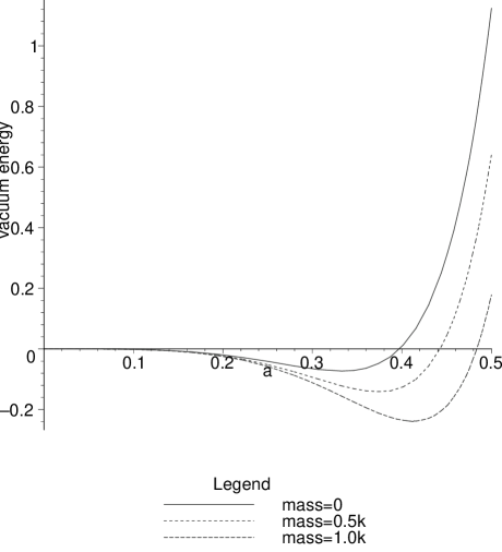
FIG. 1.: The fermion vacuum energy plotted against $a=\exp(-\pi kr)$ for various fermion masses and type $I$ boundary conditions. The vacuum energy is in units of $10^{3}k^{4}$ and shifted to vanish at $a=0$ to aid comparison. The brane tension $V_{v}$ is kept constant.

REFERENCES

- [1] T. Kaluza, Sitzungsber. Preuss. Akad. Wiss. Berlin, Math. Phys. Kl. (1921) 966.
- [2] O. Klein, Z. Phys. 37 (1926) 895; Nature (London) 118 516.
- [3] B. S. DeWitt, in Relativity, Groups, and Topology, edited by C. DeWitt and B. S. DeWitt (Gordon and Breach, New York, 1964).
- [4] E. Witten, Nucl. Phys. B 186 (1981) 412.
- [5] W. Nahm, Nucl. Phys. B 135 (1978) 149.
- [6] M. J. Duff, B. Nilsson, and C. N. Pope, Phys. Rep. 130 (1986) 1 .
- [7] N. Arkani-Hamed, S. Dimopoulos, G. Dvali, Phys. Lett. B429 (1998) 263; I. Antoniadis, N. Arkani-Hamed, S. Dimopoulos, G. Dvali, Phys. Lett. B436 (1998) 257.
- [8] L. Randall and R. Sundrum, Phys. Rev. Lett. 83 (1999) 3370; ibid. 4690.
- [9] W. D. Goldberger and M. B. Wise, Phys. Rev. D60 (1999) 107505.
- [10] H. Davoudiasl, J. L. Hewett, and T. G. Rizzo, Phys. Lett. B473 (2000) 43.
- [11] A. Pomarol, Phys. Lett. B486 (2000) 153.
- [12] Y. Grossman and M. Neubert, Phys. Lett. B474 (2000) 361.
- [13] R. Kitano, Phys. Lett. B481 (2000) 39.
- [14] C. V. Chang and J. N. Ng, Phys. Lett. B488 (2000) 390.
- [15] T. Gherghetta and A. Pomarol, Nucl. Phys. B 586 (2000) 141.
- [16] S. Chang, J. Hisano, H. Nakano, N. Okada, and M. Yamaguchi, Phys. Rev. D 63 (2000) 084025.
- [17] H. Davoudiasl, J. L. Hewett, and T. G. Rizzo, Phys. Rev. D63 (2001) 075004.
- [18] S. J. Huber and Q. Shafi, Phys. Rev. D63 (2001) 045010.
- [19] A. Flachi and D. J. Toms, Phys. Lett. B491 (2000) 157.
- [20] H. Georgi, A. Grant, G. Hailu, Phys. Rev. D63 (2001) 2853.
- [21] H. Georgi, A. Grant, G. Hailu, Phys. Lett. B506 (2001) 207.
- [22] A. Lukas, P. Ramond, A. Romanino, G. G. Ross, JHEP 04 (2001) 010.
- [23] A. Flachi, I. G. Moss, D. J. Toms, .
- [24] S. Randjbar-Daemi, M. Shaposhnikov, Phys. Lett. B492 (2000) 361.
- [25] G. Gibbons, R. Kallosh, A. Linde, JHEP 01 (2001) 022.
- [26] P. Candelas and S. Weinberg, Nucl. Phys. B237 (1984) 397.
- [27] D. J. Toms, Phys. Lett. B129 (1983) 31.
- [28] D. J. Toms, in An Introduction to Kaluza-Klein Theories, edited by H. C. Lee (World Scientific, Singapore, 1984).
- [29] Modern Kaluza-Klein Theories, edited by T. Appelquist, A. Chodos, P.G.O. Freund (Addison-Wesley, 1987).
- [30] J. Garriga, O. Pujolàs, and T. Tanaka, .
- [31] D. J. Toms, Phys. Lett. B484 (2000) 149.
- [32] W. D. Goldberger and I. Z. Rothstein, Phys. Lett. B491 (2000) 339.
- [33] A. Flachi and D. J. Toms, .
- [34] E. Ponton, E. Poppitz, .
- [35] M. Fabinger, P. Horava, Nucl. Phys. B 580 (2000) 243.
- [36] P. B. Gilkey, J. Diff. Geom. 10 (1975) 601.
- [37] T. P. Branson, P. B. Gilkey, K. Kirsten, D. V. Vassilevich, Nucl. Phys. B563 (1999) 603.
- [38] K. Kirsten, Class. Quantum Grav. 15 (1998) L5.
- [39] P. B. Gilkey, K. Kirsten, D. V. Vassilevich, Nucl. Phys. B601 (2001) 125.
- [40] I. G. Moss, Phys. Lett. B491 (2000) 203.
- [41] M. Bordag, D. V. Vassilevich, J. Phys. A 32 (1999) 8247.
- [42] S.R. Huggins, G. Kunstatter, H.P. Leivo, D.J. Toms, Phys. Rev. Lett. 58 (1987) 296; Nucl. Phys. B301 (1988) 627.
- [43] J. E. Kim, B. Kyae and H. M. Lee, Phys. Rev. D62 (2000) 045013.
- [44] J. E. Kim, B. Kyae and H. M. Lee, Nucl. Phys. B582 (2000) 296.
- [45] O. Corradini and Z. Kakushadze, Phys. Lett. B494 (2000) 302.
- [46] S. Nojiri and S. D. Odintsov, JHEP 07 (2000) 049.
- [47] N. Navromatos and J. Rizos, Phys. Rev. D62 (2000) 124004.
- [48] I. P. Neupane, JHEP 09 (2000) 040.
- [49] I. Low and A. Zee, Nucl. Phys. B585 (2000) 395.
- [50] L. Parker, D. J. Toms, Phys. Rev. D31 (1985) 953.
- [51] M. Bordag, E. Elizalde, K. Kirsten, J. Math. Phys. 37 (1996) 895.
- [52] M. Bordag, K. Kirsten, J. S. Dowker, Comm. Math. Phys. 182 (1996) 371.
- [53] A. Higuchi, L. Parker, Phys. Rev. D37 (1988) 2853.
- [54] Y. Hosotani, Ann. Phys. 190 (1989) 233; Phys. Lett. B126 (1983) 309.
- [55] D. J. Toms, Phys. Lett. B126 (1983) 445.
- [56] L. H. Ford, Phys. Rev. D21 (1980) 933.
- [57] J. S. Dowker, S. Jadhav, Phys. Rev. D39 (1989) 1196; ibid. 1196.
- [58] S. Mignemi, I. G. Moss, Phys. Rev. D48 (1993) 3725.