UT-944

hep-th/0106068

June, 2001

Survey of the Tachyonic Lump
in Bosonic String Field Theory

Kazuki Ohmori
Department of Physics, Faculty of Science, University of Tokyo
Hongo 7-3-1, Bunkyo-ku, Tokyo 113-0033, Japan

We study some properties of the tachyonic lumps in the level truncation scheme of bosonic cubic string field theory. We find that several gauges work well and that the size of the lump as well as its tension is approximately independent of these gauge choices at level (2,4). We also examine the fluctuation spectrum around the lump solution, and find that a tachyon with $\alpha^{\prime}m^{2}=-0.96$ and some massive scalars appear on the lump world-volume. This result strongly supports the conjecture that a codimension 1 lump solution is identified with a D-brane of one lower dimension within the framework of bosonic cubic string field theory.

1 Introduction

In the past years, the tachyonic lump solutions [1, 2, 3, 4] as well as the tachyon potential [6, 7, 8] have been worked out in bosonic cubic string field theory [9] using the level truncation scheme. However, these calculations were carried out only in the Feynman-Siegel gauge. Although its validity has been checked in [14], it would be interesting to see whether other gauge choices are possible. In fact, it has recently been found in [15] that the Feynman-Siegel gauge condition has a finite range of validity, and that some other gauge choices lead to similar tachyon potentials to that in the Feynman-Siegel gauge. It is the problem of choosing the gauge fixing condition(s) that we will address in the first half of this paper. We will see that we can successfully construct lump solutions with nearly correct tensions in several gauges, and that the widths of the lumps are independent of these gauge chioces at least at level (2,4).

Concerning this point, in the recent studies of so-called ‘vacuum string field theory’[16, 17, 18] it was guessed that the width of the lump solution was a gauge-dependent quantity [17]. In more detail, let us consider the center-of-mass coordinate $x^{\mu}$ of the string and its conjugate momentum $p^{\mu}$, obeying the canonical commutation relation

$$[\widehat{x}^{\mu},\widehat{p}^{\nu}]=i\eta^{\mu\nu}.$$ (1)

Combining these two operators, we can move to the oscillator representation [19] of the zero modes as [17]

$$a_{0}^{\mu}=\frac{1}{2}\sqrt{b}\widehat{p}^{\mu}-\frac{i}{\sqrt{b}}\widehat{x}^{\mu},\quad a_{0}^{\mu\dagger}=\frac{1}{2}\sqrt{b}\widehat{p}^{\mu}+\frac{i}{\sqrt{b}}\widehat{x}^{\mu}.$$ (2)

It is easily found that they satisfy the commutation relation $[a_{0}^{\mu},a_{0}^{\nu\dagger}]=\eta^{\mu\nu}$ for the creation-annihilation operators irrespective of the value of the newly introduced parameter $b$. Moreover, it has been observed in [17] that the value of the ratio of the lump tensions seems to converge to the expected single value for all $b$, while the extent of the lump in spacetime clearly depends on $b$. From these facts, the authors of [17] has proposed that the solutions of different widths are related to each other by the gauge transformation which does not affect the ghost part of the string field. Though our result suggests that the size of the lump cannot be changed by gauge transformation in the ‘ordinary’ cubic string field theory, it does not immediately contradict the above proposal because the relation between vacuum string field theory and the ordinary cubic string field theory is yet to be clarified. Since some of the symmetries in the closed string vacuum are broken in a D-brane background, it is conceivable that the ordinary cubic string field theory we will use has fewer gauge degrees of freedom than the vacuum string field theory. If the gauge symmetry which actually changes the width of the lump is broken in the presence of a D-brane background, we cannot see such an effect using the ordinary cubic open string field theory on a D-brane.

In the second half of this paper, we consider the fluctuation spectrum around the codimension-1 lump solution constructed in the modified level truncation scheme [3]. By now, it has been verified that the spacetime-independent non-perturbative vacuum solution in the ordinary cubic string field theory does not support any perturbative open string excitations [20] within the level truncation scheme. On the other hand, if the conjecture that the tachyonic lump solutions represent the lower-dimensional D-branes [21] is true, the fluctuation spectrum around the lump solution should agree with that of the corresponding D-brane. Analyses of this kind have so far been done in the tachyonic $\phi^{3}$ scalar field theory model [1, 4], the result being that the spectrum on the lump contains a tachyon with $\alpha^{\prime}m^{2}=-5/4$, a massless scalar and an approximately massless gauge field (it is reviewed in section 4.1 of [12]). At this level of approximation, the mass of the tachyon is not so close to the expected value $\alpha^{\prime}m^{2}=-1$ and the tension of the lump is only 78% of the correct answer. We will examine the fluctuation spectrum on the lump solution to a higher degree of accuracy by taking into account the scalar component fields at level 2, and find that there is a tachyon with mass $\alpha^{\prime}m^{2}\simeq-0.96$.

This paper is organized as follows. In section 2 we discuss the dependence of the tachyonic lump on the gauge choice at level (2,4) approximation. In section 3, we determine the low-lying mass spectrum around the lump solution in the Feynman-Siegel gauge, and find that a tachyon appears with the nearly correct mass squared. Section 4 includes a summary of our results and discussions on some points. Numerical data for expectation values and quite lengthy expressions for the action are collected in Appendices.

2 Tachyonic Lumps in Various Gauges

In this section we study the dependence of the lump solutions on the gauge choice. We consider the possibility of imposing gauge fixing conditions other than the Feynman-Siegel gauge $b_{0}|\Phi\rangle=0$ on the string field as well as that of leaving the gauge unfixed.

In the modified level truncation scheme introduced in [3], momentum in the $X$-direction, in which we will construct non-trivial field configurations, is discretized as $p=n/R$ with $n$ integer by compactifying the $X$-direction on a circle of radius $R$. This compact momentum is taken to contribute to the level as

$$\mathrm{level}=\frac{\alpha^{\prime}}{R^{2}}n^{2}+h_{N}+1,$$ (3)

where $h_{N}$ denotes the conformal weight of the state excluding the contribution from the momentum factor. (For more details, see [3] and chapter 4 of [12].) To this end, we consider the level (2,4) truncation approximation. At this level, the string field without gauge fixing, restricted to the twist-even sector, is expanded as

$$|\Phi\rangle=\sum_{n}\phi_{n}\ c_{1}|n\rangle+u\ c_{-1}|0\rangle+v\ L_{-2}^{X}c_{1}|0\rangle+w\ L_{-2}^{\mathcal{M}}c_{1}|0\rangle+r\ b_{-2}c_{0}c_{1}|0\rangle,$$ (4)

where $|n\rangle=e^{i\frac{n}{R}X(0)}|0\rangle$ and $|0\rangle$ is the $SL(2,\mathbf{R})$-invariant vacuum. We have denoted by $\mathcal{M}$ the 25-dimensional manifold excluding $X$, and by $L_{m}^{\mathcal{M}}$ the Virasoro generators of the conformal field theory of central charge 25 associated with $\mathcal{M}$. In finding the lump solution which is symmetric under the reflection $X\to-X$, we can put the following constraints on $\phi_{n}$’s,

$$\phi_{0} = \tau_{0},$$ (5)

$$\phi_{n} = \phi_{-n}=\frac{1}{2}\tau_{n}\qquad\mathrm{for}\quad n\geq 1,$$

so that $\phi_{n}|n\rangle+\phi_{-n}|-n\rangle=\tau_{n}\cos\frac{n}{R}X(0)|0\rangle$. The range of $n$ over which the summation in eq.(4) is taken depends on the value of $R$. In this section our choices of $R$ are $\sqrt{3\alpha^{\prime}}$ and $2\sqrt{2\alpha^{\prime}}$, in which cases

$$-2\leq n\leq 2\quad \mathrm{for} \ R=\sqrt{3\alpha^{\prime}},$$

$$-4\leq n\leq 4\quad \mathrm{for} \ R=2\sqrt{2\alpha^{\prime}},$$ (6)

at level 2. Due to the reality condition $(\mathrm{bpz}|\Phi\rangle)^{\dagger}=|\Phi\rangle$ on the string field, the component fields $\tau_{n},u,v,w,r$ must be real.

Substituting the level-expanded string field (4) into the cubic action

$$S=-\frac{1}{g_{o}^{2}}\left(\frac{1}{2}\langle\Phi|Q_{B}|\Phi\rangle+\frac{1}{3}\langle\Phi,\Phi,\Phi\rangle\right)$$ (7)

on a D$p$-brane, we have found the level (2,4) truncated gauge-unfixed action to be

$$\frac{-g_{o}^{2}S}{2\pi RV_{p}} = -\frac{1}{2}\tau_{0}^{2}+\sum_{n\geq 1}\frac{1}{4}\left(\frac{\alpha^{\prime}}{R^{2}}n^{2}-1\right)\tau_{n}^{2}-\frac{1}{2}u^{2}+\frac{1}{4}v^{2}+\frac{c^{\mathcal{M}}}{4}w^{2}+2r^{2}-3ur$$ (8)

$${}+\frac{1}{2}vr+\frac{c^{\mathcal{M}}}{2}wr+\frac{1}{3}\sum\delta_{n_{1}+n_{2}+n_{3}}K^{3-\frac{\alpha^{\prime}}{R^{2}}(n_{1}^{2}+n_{2}^{2}+n_{3}^{2})}\phi_{n_{1}}\phi_{n_{2}}\phi_{n_{3}}$$

$$+K^{3}\Biggl{[}\frac{11}{27}\tau_{0}^{2}u+\frac{11}{54}\sum_{n\geq 1}K^{-\frac{2\alpha^{\prime}}{R^{2}}n^{2}}\tau_{n}^{2}u$$

$$\qquad-\frac{5}{54}\tau_{0}^{2}v+\frac{1}{2}\sum_{n\geq 1}\left(\frac{16\alpha^{\prime}}{27R^{2}}n^{2}-\frac{5}{54}\right)K^{-\frac{2\alpha^{\prime}}{R^{2}}n^{2}}\tau_{n}^{2}v$$

$$\qquad-\frac{5}{54}c^{\mathcal{M}}\ \tau_{0}^{2}w-\frac{5}{108}c^{\mathcal{M}}\sum_{n\geq 1}K^{-\frac{2\alpha^{\prime}}{R^{2}}n^{2}}\tau_{n}^{2}w$$

$$\qquad-\frac{16}{27}\tau_{0}^{2}r-\frac{8}{27}\sum_{n\geq 1}K^{-\frac{2\alpha^{\prime}}{R^{2}}n^{2}}\tau_{n}^{2}r$$

$$\qquad+\frac{19}{243}\tau_{0}u^{2}+\frac{179}{972}\tau_{0}v^{2}+\frac{c^{\mathcal{M}}}{729}\left(\frac{25}{4}c^{\mathcal{M}}+128\right)\tau_{0}w^{2}+\frac{64}{243}\tau_{0}r^{2}$$

$$\qquad-\frac{55}{729}\tau_{0}uv-\frac{55}{729}c^{\mathcal{M}}\ \tau_{0}uw+\frac{32}{81}\tau_{0}ur$$

$$\qquad+\frac{25}{1458}c^{\mathcal{M}}\ \tau_{0}vw+\frac{80}{729}\tau_{0}vr+\frac{80}{729}c^{\mathcal{M}}\ \tau_{0}wr\Biggr{]},$$

where $c^{\mathcal{M}}=25$, $K=3\sqrt{3}/4$, and note that our normalization convention is such that every component field is dimensionless and that we are not setting $\alpha^{\prime}$ to any fixed value. In spite of leaving the gauge degrees of freedom unfixed, the procedure of level truncation actually breaks the gauge invariance, so that the equations of motion obtained by varying the action (8) have a discrete set of solutions, instead of a continuous family. Hence we can find the isolated ‘closed string vacuum’ solution and the lump solutions for two values (6) of radius by solving the simultaneous equations of motion numerically, even without any gauge fixing. The expectation values found this way are given in Table 2 in Appendix A. Putting these values back to the above action, we can obtain the numerical values for the depth of the tachyon potential and for the tensions of the lump solutions using the following formulae [3, 12], respectively,

$$f(\Phi_{\mathrm{vac}}) \equiv -\frac{S(\Phi_{\mathrm{vac}})}{2\pi RV_{p}\tau_{p}}=2\pi^{2}\times\mbox{(r.h.s. of eq.(\ref{eq:H}))},$$ (9)

$$r(R,\Phi_{\mathrm{lump}}) = \frac{R}{\sqrt{\alpha^{\prime}}}\Bigl{(}f(\Phi_{\mathrm{lump}})-f(\Phi_{\mathrm{vac}})\Bigr{)},$$ (10)

where we have denoted by $\tau_{p}$ the tension of the original D$p$-brane, by $\Phi_{\mathrm{vac}}$ the closed string vacuum configuration of the string field, and by $\Phi_{\mathrm{lump}}$ the lump configuration. We have used the relation [24]

$$\tau_{p}=\frac{1}{2\pi^{2}g_{o}^{2}}$$

between the D$p$-brane tension and the open string coupling on the D$p$-brane in the most right hand side of eq.(9). The conjectured values for $-f(\Phi_{\mathrm{vac}})$ and $r(^{\forall}\!R,\Phi_{\mathrm{lump}})$ are 1. Our results obtained with the gauge left unfixed are

$$f(\Phi_{\mathrm{vac}})=-0.885220,\quad r(\sqrt{3\alpha^{\prime}},\Phi_{\mathrm{lump}})=0.869597,\quad r(\sqrt{8\alpha^{\prime}},\Phi_{\mathrm{lump}})=0.679800.$$ (11)

These values are summarized in Table 1, together with the gauge-fixed ones to be explained below.

Next we consider fixing the gauge. As we mentioned above, the gauge invariance has actually been broken by the level truncation. However, this breakdown is not under control so that the gauge-fixing is needed to obtain more definite results. The first gauge fixing condition we try to choose is the Feynman-Siegel gauge

$$b_{0}|\Phi\rangle=0,$$ (12)

whose validity at the linearized level was established in [7], and its range of validity in the non-perturbative case has been argued in [15]. In terms of the component fields appearing in eq.(4), this condition is restated simply as

$$r=0.$$ (13)

As alternatives we consider the following three choices

$$b_{1}|\Phi\rangle = 0,$$

$$L_{2}^{X}|\Phi\rangle = 0,$$ (14)

$$L_{2}^{\mathcal{M}}|\Phi\rangle = 0,$$

whose component forms are, respectively,

$$u = 0,$$

$$v = 0,$$ (15)

$$w = 0,$$

as suggested in [15]. The validity of these gauges at the linearized level can be verified in a similar way to the case of the Feynman-Siegel gauge, at least in the level (2,4) truncation scheme. To give an example, let us look at the $b_{1}$-gauge closely. Suppose that the initial string field $|\Phi\rangle$ is not annihilated by $b_{1}$. Acting on $|\Phi\rangle$ with the linearized gauge transformation, we reach the transformed field

$$|\widetilde{\Phi}\rangle=|\Phi\rangle-Q_{B}|\Lambda\rangle,$$ (16)

where the gauge parameter $|\Lambda\rangle$ must have ghost number 0. If $|\Lambda\rangle$ is taken to satisfy

$$b_{1}|\Lambda\rangle=0\quad\mathrm{and}\quad L_{1}^{\mathrm{tot}}|\Lambda\rangle=b_{1}|\Phi\rangle,$$ (17)

then it follows that

$$b_{1}|\widetilde{\Phi}\rangle = b_{1}|\Phi\rangle-b_{1}Q_{B}|\Lambda\rangle=b_{1}|\Phi\rangle-\{b_{1},Q_{B}\}|\Lambda\rangle$$

$$= b_{1}|\Phi\rangle-L_{1}^{\mathrm{tot}}|\Lambda\rangle=0,$$

so we have found that there is a representative obeying the gauge fixing condition $b_{1}|\widetilde{\Phi}\rangle=0$ in each gauge equivalent class, if there exists a suitable gauge parameter $|\Lambda\rangle$ satisfying (17). The string field $|\Lambda\rangle$ of ghost number 0 is expanded as

$$|\Lambda\rangle=\sum_{n}\lambda_{n}\ b_{-1}c_{1}|n\rangle+\sum_{n}\mu_{n}\ b_{-2}c_{1}|n\rangle+\sum_{n\neq 0}\nu_{n}\ L_{-1}^{X}b_{-1}c_{1}|n\rangle+\cdots.$$

Since we are focusing on the even level fields thanks to the twist symmetry, the first term (at oscillator level 1) can be dropped. In addition, the third and the still higher terms do not contribute at level 2. Therefore, we have only to consider the 1-parameter gauge degree of freedom

$$|\Lambda\rangle=\mu\ b_{-2}c_{1}|0\rangle$$ (18)

at this level of approximation. It is easily found that the above $|\Lambda\rangle$ satisfies both conditions in (17) if we take $\mu$ to be equal to $u/3$. Furthermore, it is obvious that there is no residual gauge degree of freedom after fixing the value of $\mu$. Similarly, we can reach the $L_{2}^{X}$- and $L_{2}^{\mathcal{M}}$-gauge by taking $\mu=v$ and $\mu=w$, respectively, with no residual gauge degrees of freedom left unfixed. Putting aside the problem on the validity of these gauge fixing conditions at higher levels, we will try to construct lump solutions as well as the tachyon potential using these gauge choices. And we will test one more gauge fixing condition

$$B|\Phi\rangle\equiv\left(b_{0}+\frac{1}{2}(b_{2}+b_{-2})\right)|\Phi\rangle=0$$ (19)

which was proposed in [16] as a modified version of the Feynman-Siegel gauge. This modification is necessary in vacuum string field theory with a non-standard BRST operator $\mathcal{Q}$ made purely out of ghost operators because of the problems described in [16]. Though the ordinary cubic string field theory has no problem about the Feynman-Siegel gauge, it is worth trying it in our context. Written in terms of the component fields, $B|\Phi\rangle=0$ gives

$$r=\frac{1}{2}\tau_{0}.$$ (20)

After putting the gauge fixing conditions (13),(15) or (20) on the action (8), we look for solutions by extremizing the resulting action with respect to the remaining field variables. The field values which solve the equations of motion are shown in Table 2–4 in Appendix A, and the values of the lump tensions are displayed in Table 1.

gauge	depth of	lump tension	lump tension
	the potential	for $R=\sqrt{3\alpha^{\prime}}$	for $R=\sqrt{8\alpha^{\prime}}$
left unfixed	$-0.885220$	0.869597	0.679800
Feynman-Siegel	$-0.948553$	$1.02368\phantom{0}$	$1.04513\phantom{0}$
$b_{1}|\Phi\rangle=0$	$-0.894765$	0.985080	$1.04153\phantom{0}$
$L_{2}^{X}|\Phi\rangle=0$	$-0.926410$	0.958814	0.959953
$L_{2}^{\mathcal{M}}|\Phi\rangle=0$	$-0.900681$	0.994212	$1.04559\phantom{0}$
$B|\Phi\rangle=0$	$-0.935830$	$1.21536\phantom{0}$	$1.51654\phantom{0}$

Table 1: The numerical values of the depth $f(\Phi_{\mathrm{vac}})$ of the tachyon potential and those of the lump tensions $r(R,\Phi_{\mathrm{lump}})$ for various gauge choices, at level (2,4) approximation.

From this table, it seems that the middle four gauges are working pretty well, whereas there is something wrong with the $B$-gauge and the non-gauge-fixed one in constructing lumps.

Given the fact that the reasonable values for the tension of the lump are reproduced in four cases, we wish to compare the profiles of the tachyon field given by

$$t(x)=\sum_{n\in\mathbf{Z}}\phi_{n}e^{i\frac{n}{R}x}=\sum_{n\in\mathbf{Z}_{\geq 0}}\tau_{n}\cos\frac{n}{R}x.$$ (21)

Substituting the expectation values shown in Table 2–4 into eq.(21), we can explicitly find the tachyon profiles in various gauges. Figure 1 and Figure 3 show them put side by side, for $R=\sqrt{3\alpha^{\prime}}$ and $R=\sqrt{8\alpha^{\prime}}$ respectively. And, these profiles are superposed in Figure 2 and in Figure 4 for each radius.

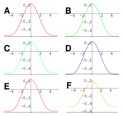
Figure 1: The tachyon profiles $-t(x)$ for $R=\sqrt{3\alpha^{\prime}}$. A: unfixed, B: Feynman-Siegel gauge, C: $u=0$, D: $v=0$, E: $w=0$, F: $B=0$. The dashed lines represent the expectation values of tachyon field at the closed string vacuum.

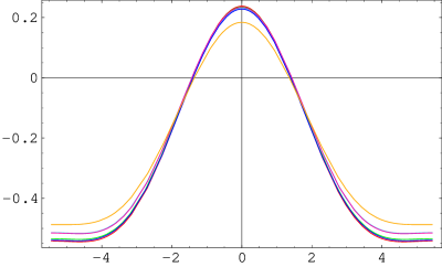
Figure 2: The tachyon profiles $-t(x)$ for $R=\sqrt{3\alpha^{\prime}}$ in various gauges.

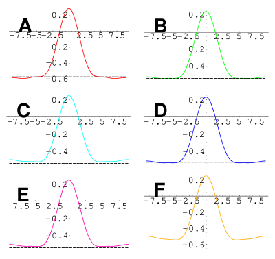
Figure 3: The tachyon profiles $-t(x)$ for $R=\sqrt{8\alpha^{\prime}}$. A: unfixed, B: Feynman-Siegel gauge, C: $u=0$, D: $v=0$, E: $w=0$, F: $B=0$. The dashed lines represent the expectation values of tachyon field at the closed string vacuum.

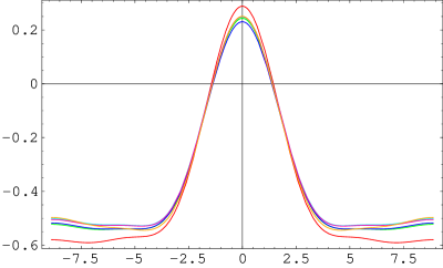
Figure 4: The tachyon profiles $-t(x)$ for $R=\sqrt{8\alpha^{\prime}}$ in various gauges.

These figures clearly indicate that the profiles found in different gauges are almost identical. To check this quantitatively, we fit each profile (21) with a Gaussian curve of the form

$$G(x)=a+be^{-\frac{x^{2}}{2\sigma^{2}}}.$$ (22)

We have found the resulting values of $\sigma$ to be

$$\left.\begin{array}[]{|c||c|c|c|c|c|c|}\hline\cr\mbox{Gauge}&\mbox{left unfixed}&\mbox{Feynman-Siegel}&b_{1}&L_{2}^{X}&L_{2}^{\mathcal{M}}&B\\ \hline\cr R=\sqrt{3\alpha^{\prime}}&1.61433&1.61608&1.61711&1.62301&1.61531&1.66272\\ \hline\cr R=2\sqrt{2\alpha^{\prime}}&1.56733&1.55317&1.53030&1.55641&1.53214&1.50111\\ \hline\cr\end{array}\right.$$ (23)

The full set of values for $(a,b,\sigma)$ is shown in Table 5 in Appendix A. As an illustration, we show in Figure 5 the result of the fitting for the solution obtained in the Feynman-Siegel gauge for $R=2\sqrt{2\alpha^{\prime}}$.

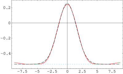
Figure 5: The result of the fitting of the lump profile $t(x)$ (solid line) with the gaussian $G(x)$ (dashed line): $R=2\sqrt{2\alpha^{\prime}}$, Feynman-Siegel gauge.

In order to estimate errors, we quote the following result from [3]:

$\sigma=1.52341$ at level (3,6) for $R=\sqrt{3\alpha^{\prime}}$ in Feynman-Siegel gauge.

Hence the error originating from the level truncation approximation is estimated to be

$$\frac{|1.61608-1.52341|}{1.61608}\simeq 0.057.$$

Since the range of the values (23) obtained in various gauges for each fixed radius is well within 6%, our result suggests that the values of $\sigma$ for lump solutions found in different gauges agree with each other. It has already been pointed out in [3] that the size $\sigma$ of the lump solution in Feynman-Siegel gauge is independent of the radius $R$. Besides, we have found that the size of the lump is also independent of the gauge choices, at least within the range of our approximation.

3 Fluctuation Spectrum Around the Tachyonic Lump

In this section, we analyze the fluctuation spectrum on the lump world-volume in the Feynman-Siegel gauge for $R=\sqrt{3\alpha^{\prime}}$: While we expect that any other gauge will do, it seems that the Feynman-Siegel gauge has a better convergence property than others in the sense of level truncation [15]. On one hand too small a value of radius makes the structure of the lump vague, and on the other hand too large a value of radius makes the calculations less accurate. In general, if we have a solution $\Phi_{0}$ to the equation of motion available, the cubic action for the fluctuation field $\Phi^{\prime}$ expanded around the solution $\Phi_{0}$ becomes

$$S(\Phi_{0}+\Phi^{\prime})=S(\Phi_{0})-\frac{1}{g_{o}^{2}}\left(\frac{1}{2}\langle\Phi^{\prime}|Q|\Phi^{\prime}\rangle+\frac{1}{3}\langle\Phi^{\prime},\Phi^{\prime},\Phi^{\prime}\rangle\right),$$

where the new kinetic operator $Q$ is defined by

$$Q\Phi^{\prime}=Q_{B}\Phi^{\prime}+\Phi_{0}*\Phi^{\prime}+\Phi^{\prime}*\Phi_{0},$$

and we can show that $Q$ is also nilpotent, $Q^{2}=0$. Hence the physical perturbative spectrum around the solution $\Phi_{0}$ is determined by the cohomology of $Q$. For the tachyon vacuum solution $\Phi_{0}=\Phi_{\mathrm{vac}}$, it has numerically been verified that $Q$ has vanishing cohomology [20] and, more strongly, it has recently been proposed that, after a suitable field redefinition, $Q$ can be brought to a simple form made purely out of ghosts [16]. On the other hand, for the codimension-1 lump solution $\Phi_{0}=\Phi_{\mathrm{lump}}$, we expect that $Q$ should be again the BRST operator such that the cohomology of $Q$ reproduces the perturbative open string spectrum on a D-brane of one lower dimension. Since, however, we have not gotten a closed form expression for $\Phi_{\mathrm{lump}}$, we will proceed with the help of the level truncation approximation. In principle, all we have to do is to rewrite the string field theory action (7) in terms of the component fields having the general momentum-dependence, to expand them about the expectation values for the lump solution, and to look for zeroes of the quadratic form for the fluctuation fields. However, the existence of the off-diagonal pieces arising from the cubic interaction terms complicates the analysis, as explained below.

To begin with, let us state our settings. The original D-brane is a space-filling D25-brane in the 26-dimensional flat spacetime, and the codimension 1 lump is, of course, to be identified with a flat D24-brane. We will focus on the scalar fields up to level 2, restricting to the twist-even sector. While it is interesting to incorporate also the twist-odd scalar fields, we will not do so because they do not mix with twist-even fields in the quadratic terms and, practically, adding these terms makes the calculations much more lengthy. Therefore, the expansion of the string field we will consider becomes

$$|\Phi\rangle = \int d^{25}\!k\Biggl{(}\sum_{n=-2}^{2}\phi_{n}(k)\ c_{1}|n,k\rangle+u(k)\ c_{-1}|0,k\rangle$$

$${}+B_{MN}(k)\ \alpha_{-1}^{M}\alpha_{-1}^{N}c_{1}|0,k\rangle+i\check{B}_{M}(k)\ \alpha_{-2}^{M}c_{1}|0,k\rangle\Biggr{)},$$

where $k$ is the 25-dimensional momentum vector along $\mathcal{M}$, $|n,k\rangle=e^{i\frac{n}{R}X(0)+ik_{\mu}X^{\mu}(0)}|0\rangle$, and $M,N$ run from 0 to 25, while $\mu,\nu$ from 0 to 24 $(X\equiv X^{25})$. For simplicity, we have assumed that $\mathcal{M}$ is non-compact flat $\mathbf{R}^{1,24}$ ignoring the problem that the D-brane has an infinite mass, which would be resolved by compactifying all the space directions on a torus of large radii. The reality conditions

$$\phi_{n}(k)^{*}=\phi_{-n}(-k),\quad u(k)^{*}=u(-k),\quad B_{MN}(k)^{*}=B_{MN}(-k),\quad\check{B}_{M}(k)^{*}=\check{B}_{M}(-k)$$ (25)

follow from the reality condition imposed on the string field. In this representation, the expectation values of the fields corresponding to the lump solution take the forms

$$\overline{\phi_{0}(k)} = \overline{\tau_{0}}\delta^{25}(k),$$

$$\overline{\phi_{\pm n}(k)} = \overline{\phi_{\pm n}}\delta^{25}(k)=\frac{1}{2}\overline{\tau_{n}}\delta^{25}(k)\qquad\mathrm{for}\ \ n=1,2,$$

$$\overline{u(k)} = \overline{u}\delta^{25}(k),$$ (26)

$$\overline{\check{B}_{M}(k)} = 0,$$

$$\overline{B_{MN}(k)} = \left(\begin{array}[]{c|c}\frac{\overline{w}}{2}\eta^{(25)}_{\mu\nu}&0\\ \hline\cr 0&\frac{\overline{v}}{2}\end{array}\right)\delta^{25}(k),$$ (29)

where $(\overline{\tau_{n}},\overline{u},\overline{v},\overline{w})$ are given in Table 2 for the Feynman-Siegel gauge, $R=\sqrt{3\alpha^{\prime}}$. The reason why we are retaining the vector and the tensor fields in eq.(3) is that the longitudinal components of them and the trace of $B_{\mu\nu}$, as well as the transverse ($X$-)components, behave as scalars and mix with $\phi_{n}$ and $u$. We almost follow the conventions of [6], but with a slight difference encountered later.

Substituting the string field (3) into the cubic action (7) again, we have obtained the level (2,4)-truncated action written in terms of the component fields. We write down the explicit expression of it in Appendix B: we have derived it using the technology of conservation laws developed in [26]. Given this expression, we can obtain the action for the fluctuation fields by shifting the original fields by their expectation values (26) as

$$\phi_{n}(k)\to\overline{\phi_{n}(k)}+\phi_{n}(k),\quad u(k)\to\overline{u(k)}+u(k),\quad\cdots$$ (30)

with a slight abuse of notation. Now, we do not impose the constraints $\phi_{n}=\phi_{-n}$ on $\phi_{n}$’s because $\phi_{n}$ and $\phi_{-n}$ are distinct fields carrying the opposite Kaluza-Klein charge to each other. We discuss here the Lorentz decompositions of the vector and the tensor fluctuation fields, according to [6]. The massive vector field $\check{B}_{\mu}(k)$ whose polarization is tangential to the lump is divided into the longitudinal and the transverse parts as

$$\check{B}_{\mu}(k) = \check{B}^{L}_{\mu}(k)+\check{B}_{\mu}^{T}(k),$$

$$\check{B}_{\mu}^{L}(k) = \frac{k_{\mu}}{ik^{2}}ik^{\nu}\check{B}_{\nu}(k).$$ (31)

It is easily found that

$$k^{\mu}\check{B}_{\mu}(k)=k^{\mu}\check{B}_{\mu}^{L}(k),\quad k^{\mu}\check{B}_{\mu}^{T}(k)=0.$$

We further define

$$\mathcal{B}^{L}(k)\equiv i\sqrt{\alpha^{\prime}}k^{\nu}\check{B}_{\nu}(k),$$ (32)

which can be regarded as a scalar in addition to the $X$-th vector component $\check{B}_{X}(k)$ transverse to the lump, and satisfies the reality condition

$$\mathcal{B}^{L}(k)^{*}=-i\sqrt{\alpha^{\prime}}k^{\nu}\check{B}_{\nu}(k)^{*}=i\sqrt{\alpha^{\prime}}(-k)^{\nu}\check{B}_{\nu}(-k)=\mathcal{B}^{L}(-k).$$

Using this definition, it follows that

$$\check{B}_{\mu}(k)\check{B}^{\mu}(-k)=\check{B}_{\mu}^{T}(k)\check{B}^{T\mu}(-k)+\frac{1}{\alpha^{\prime}k^{2}}\mathcal{B}^{L}(k)\mathcal{B}^{L}(-k).$$ (33)

Note that the $\mathcal{B}^{L}$-field has non-standard normalization, though it will not affect our analysis. In what follows, we will discard the first term in the right hand side of (33). Similarly, the tensor field $B_{MN}(k)$ is decomposed into several parts according to their Lorentz transformation properties as

• $XX$ component: $B_{XX}(k)$,

• longitudinal component of the ‘Kaluza-Klein’ vector $B_{\mu X}(k)$:

  $$B^{L}_{\mu X}(k)=\frac{k_{\mu}}{ik^{2}}\frac{\beta^{L}_{X}(k)}{\sqrt{\alpha^{\prime}}};\quad\beta^{L}_{X}(k)\equiv i\sqrt{\alpha^{\prime}}k^{\nu}B_{\nu X}(k),$$ (34)

  $$B_{\mu X}(k)B^{\mu X}(-k)\longrightarrow\frac{1}{\alpha^{\prime}k^{2}}\beta^{L}_{X}(k)\beta^{L}_{X}(-k),$$

• trace part of $B_{\mu\nu}(k)$: $\eta^{\mu\nu}_{(25)}B_{\mu\nu}(k)\equiv\sqrt{25}B(k)$,

  $$B_{\mu\nu}(k)=b_{\mu\nu}(k)+\frac{1}{5}\eta^{(25)}_{\mu\nu}B(k),$$ (35)

  ($b_{\mu\nu}$ is the traceless part of $B_{\mu\nu}$),

• longitudinal part of $b_{\mu\nu}(k)$:

  $$b^{LL}(k)\equiv\frac{k^{\rho}k^{\sigma}}{k^{2}}b_{\rho\sigma}(k),\quad b^{LL}_{\mu\nu}(k)=\frac{k_{\mu}k_{\nu}}{k^{2}}b^{LL}(k),$$ (36)

• and two transverse vectors and a symmetric 2-tensor.

Then we have

$$B_{\mu\nu}(k)B^{\mu\nu}(-k) \mathop{\longrightarrow}\limits^{\mathrm{scalar}} B(k)B(-k)+b^{LL}(k)b^{LL}(-k),$$

$$k^{\mu}k^{\nu}B_{\mu\nu}(k) = k^{2}b^{LL}(k)+\frac{1}{5}k^{2}B(k).$$

Collecting the pieces above, there are 12 scalar fields we have to consider up to level 2 from the point of view of the lump world-volume, namely

$$V^{T}=\biggl{(}\phi_{2},\ \phi_{1},\ \phi_{0},\ \phi_{-1},\ \phi_{-2},\ u,\ \check{B}_{X},\ \mathcal{B}^{L},\ B_{XX},\ \beta^{L}_{X},\ B,\ b^{LL}\biggr{)}$$ (37)

in the vector notation with $T$ denoting the transposition.

In the action for the fluctuation fields expanded around the lump solution, there are quadratic terms of the form

$$(\mathrm{vev})\cdot(\mathrm{field})\cdot(\mathrm{field}^{\prime})$$

arising from the cubic interaction terms in the original action. Since the whole set of the cubic interaction terms includes almost all of the possible couplings, the quadratic form for the fluctuation fields is not diagonalized at all. Using the notation introduced above, the quadratic form can generally be written as

$$(2\pi)^{26}R\int d^{25}k\ V^{\dagger}(-k)M(k^{2})V(k)$$ (38)

where the ‘quadratic form matrix’ $M$ is Hermitian and

$$V^{\dagger}=\biggl{(}\phi_{-2},\ \phi_{-1},\ \phi_{0},\ \phi_{1},\ \phi_{2},\ u,\ \cdots\biggr{)}.$$

Hence we can determine the scalar fluctuation spectrum on the lump by finding the set of values of $m^{2}=-k^{2}$ at which one (or some) of the eigenvalues of the $12\times 12$ matrix $M(k^{2})$ vanishes. The explicit expressions for the components $M_{ij}$ of the matrix $M$ are displayed in Appendix C. Instead of diagonalizing this huge matrix, we have calculated the determinant of $M$ and looked for the values of $m^{2}=-k^{2}$ at which $\det M$ vanishes. We have plotted $\det M$ as a function of $\mu\equiv-\alpha^{\prime}k^{2}$ in Figure 6–10: We had to divide the whole curve into several sectors because the scale of $\det M$ greatly changes from place to place.

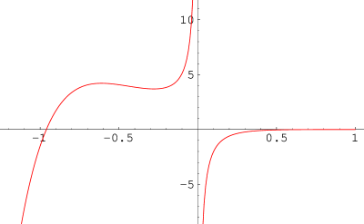
Figure 6: The plot of $\det M$ as a function of $\mu=-\alpha^{\prime}k^{2}\in[-1.2\ ,\ 1]$.

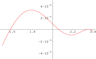
Figure 7: The plot of $\det M$ as a function of $\mu=-\alpha^{\prime}k^{2}\in[1.5\ ,\ 2.4]$.

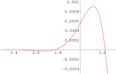
Figure 8: The plot of $\det M$ as a function of $\mu=-\alpha^{\prime}k^{2}\in[2.3\ ,\ 3.3]$.

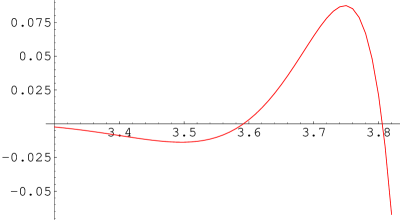
Figure 9: The plot of $\det M$ as a function of $\mu=-\alpha^{\prime}k^{2}\in[3.3\ ,\ 3.82]$.

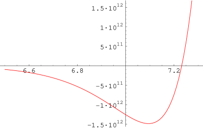
Figure 10: The plot of $\det M$ as a function of $\mu=-\alpha^{\prime}k^{2}\in[6.5\ ,\ 7.3]$.

The seeming divergence of $\det M$ at $k^{2}=0$ (Figure 6) is an artifact caused by the non-standard normalizations of $\mathcal{B}^{L}$ and $\beta^{L}_{X}$. The numerical values of $\mu=\alpha^{\prime}m^{2}=-\alpha^{\prime}k^{2}$ where the $\det M$ vanishes have turned out to be

$$\left.\begin{array}[]{|c|c|c|c|c|c|}\hline\cr\mathrm{1st}&\mathrm{2nd}&\mathrm{3rd}&\mathrm{4th}&\mathrm{5th}&\mathrm{6th}\\ \hline\cr-0.960696&1.57958&2.06040&2.34365&2.36161&2.76601\\ \hline\cr\end{array}\right.$$

$$\left.\begin{array}[]{|c|c|c|c|c|}\hline\cr\mathrm{7th}&\mathrm{8th}&\mathrm{9th}&\mathrm{10th}&\mathrm{11th}\\ \hline\cr\ 3.22656&3.59172&3.80594&7.23182&\ \ 22.1\\ \hline\cr\end{array}\right..$$

The first point we should note is that there exists only one tachyonic state whose mass squared $\alpha^{\prime}m^{2}\simeq-0.961$ is very close to the expected value $(\alpha^{\prime}m^{2}=-1)$! One may take it for granted that the properties of the original tachyon persist to the lump, but it is not correct because the tachyon field living on the lump world-volume is not identical to the original tachyon $\phi$ on the D25-brane at all. In fact, we must take suitable linear combinations of the fluctuation fields to diagonalize the matrix $M(k^{2})$. Explicitly, the lump tachyon $\varphi$ takes the form

$$\varphi = 0.119537\ \phi_{2}+0.478126\ \phi_{1}+0.715829\ \phi_{0}+0.478126\ \phi_{-1}+0.119537\ \phi_{-2}$$

$${}+0.00234923\ u-0.00332686\ \mathcal{B}^{L}+0.0398185\ B_{XX}-0.0127727\ B+0.00604012\ b^{LL}.$$

As we increase the level of approximation, more and more fields take part in constructing the lump tachyon, though their contribution will be small. Hence, our result that there is a tachyon with $\alpha^{\prime}m^{2}\simeq-0.96$ on the lump world-volume is not only desirable but also quite non-trivial.

The second point is that there are also several zeroes around $\alpha^{\prime}m^{2}=2$. Although some of these states may be $Q$-exact and hence not physical, we have not pursued this issue because the $Q$-exactness here is less significant than in the case of the tachyon vacuum. The spectrum on a D24-brane contains degenerate scalar states at $\alpha^{\prime}m^{2}=1$ as in eq.(37), so that the appearance of the nearly degenerate states on the lump seems to be consistent with the expected spectrum, though the values of $\alpha^{\prime}m^{2}$ are a little too large: This point will be further discussed in section 4. Actually, even the fact that the $\det M$, which is a very complicated function of $\mu=-\alpha^{\prime}k^{2}$, has so many zeroes on the positive real axis is rather surprising and should not be an accident. Therefore, our result can be regarded as a strong piece of evidence that the fluctuation spectrum around the tachyonic lump solution agrees with that of a D24-brane.

4 Conclusions and Discussions

In this paper, we have discussed two issues concerned with the tachyonic lump solutions in bosonic cubic string field theory. One is the problem of whether other gauges than the Feynman-Siegel gauge may work as well and, if so, how the properties (tension, size) of the lump depend on these gauge choices. We have obtained the result that at level (2,4) we have succeeded in constructing lump solutions in various gauges except for the $B$-gauge, and that not only the tension but also the size of the lump is independent of these good gauge choices. Besides, solving the equations of motion without gauge fixing does not seem to give sensible results. It remains, however, to be resolved whether these conclusions, together with the legitimacy of the gauge fixing conditions (14) themselves, persist to the higher levels or not. The other is to find the fluctuation spectrum around the tachyonic lump. Our calculations have shown that there are a tachyon with $\alpha^{\prime}m^{2}\simeq-0.96$ and some massive scalar states on the lump, and we regard this result as one more piece of evidence that a tachyonic lump solution represents a lower-dimensional D-brane. We conclude this paper with some discussions.

In the analysis of the fluctuation spectrum, we have considered the determinant of $M$. When we increase the truncation level, however, $M$ constitutes only part of the entire quadratic form matrix

$$\widetilde{M}=\left(\begin{array}[]{cc}M&L\\ L^{\dagger}&N\end{array}\right),$$

and the masses of the states will be shifted due to the existence of non-vanishing off-diagonal block $L$, as well as the small corrections to $M$ itself. Nevertheless we expect that the qualitative features of our result will not be altered at higher levels because the contribution from $L$ is considered to be small. Indeed, since each component of $L$ comes from the cubic coupling among light fields and heavy fields, it is plausible that the coefficient of such a coupling is small. But recall that the values of $\alpha^{\prime}m^{2}(>0)$ at which $\det M$ vanishes were a little larger than the expected values. We hope that the masses of these massive states approach 1 as we increase the truncation level, whereas the mass of the tachyon scarcely changes. We cannot prove this statement because to reach the next level $\left(\frac{7}{3},\frac{14}{3}\right)$ requires us to evaluate the $26\times 26$ quadratic form matrix and its determinant, which has not been done yet.

In the case of superstring, a tachyonic kink solution on a non-BPS D-brane was constructed in [11] by applying the level truncation scheme to superstring field theory formulated by Berkovits. Since the kink solution is to be identified with a BPS D-brane of one lower dimension, the fluctuation spectrum around it is expected to contain a massless scalar field representing the translational mode of the kink, instead of a tachyon. Although the actual calculations must become much more complicated because of the interaction terms of higher orders, it would in principle be possible to repeat similar calculations to those explained in this paper, and we believe that our expectations could be verified by explicit calculations.

Appendices

A Expectation Values and Fitting of the Lumps

	Gauge unfixed			Feynman-Siegel gauge
Field	vacuum	$R=\sqrt{3\alpha^{\prime}}$	$R=\sqrt{8\alpha^{\prime}}$	vacuum	$R=\sqrt{3\alpha^{\prime}}$	$R=\sqrt{8\alpha^{\prime}}$
$\tau_{0}$	0.570140	0.261307	0.389790	0.541591	0.257030	0.366958
$\tau_{1}$	0	$-0.389854$	$-0.333837$	0	$-0.384575$	$-0.295236$
$\tau_{2}$	0	$-0.109253$	$-0.210478$	0	$-0.107424$	$-0.199225$
$\tau_{3}$	0	—	$-0.100522$	0	—	$-0.0877869$
$\tau_{4}$	0	—	$-0.0334873$	0	—	$-0.0281938$
$u$	$-0.0878149$	0.286261	0.577919	0.173264	0.0888087	0.122846
$v$	$-0.0390313$	0.0541575	0.161105	0.0518987	$-0.00675676$	0.0195679
$w$	$-0.0390313$	0.0935772	0.185541	0.0518987	0.0317837	0.0407204
$r$	0.182205	$-0.0887169$	$-0.230081$	0	0	0

Table 2: The expectation values for the closed string vacuum solution and the lump solutions for $R=\sqrt{3\alpha^{\prime}}$ and for $R=\sqrt{8\alpha^{\prime}}$ in the case of free gauge and of the Feynman-Siegel gauge.

	$b_{1}|\Phi\rangle=0$			$L_{2}^{X}|\Phi\rangle=0$
Field	vacuum	$R=\sqrt{3\alpha^{\prime}}$	$R=\sqrt{8\alpha^{\prime}}$	vacuum	$R=\sqrt{3\alpha^{\prime}}$	$R=\sqrt{8\alpha^{\prime}}$
$\tau_{0}$	0.547091	0.245390	0.354999	0.531880	0.261384	0.367602
$\tau_{1}$	0	$-0.372937$	$-0.286657$	0	$-0.383699$	$-0.289441$
$\tau_{2}$	0	$-0.103975$	$-0.200172$	0	$-0.105811$	$-0.197050$
$\tau_{3}$	0	—	$-0.0881422$	0	—	$-0.0847774$
$\tau_{4}$	0	—	$-0.0282572$	0	—	$-0.0270753$
$u$	0	0	0	0.228984	0.197288	0.216846
$v$	$-0.00986666$	$-0.0383939$	$-0.0256342$	0	0	0
$w$	$-0.00986666$	$-0.00167938$	$-0.00459855$	0.0709321	0.0657133	0.0705697
$r$	0.118928	0.0464671	0.0716666	$-0.0356672$	$-0.0484534$	$-0.0476229$

Table 3: The expectation values for the closed string vacuum solution and the lump solutions for $R=\sqrt{3\alpha^{\prime}}$ and for $R=\sqrt{8\alpha^{\prime}}$ in the case of $b_{1}$-gauge and of $L_{2}^{X}$-gauge.

	$L_{2}^{\mathcal{M}}|\Phi\rangle=0$			$B|\Phi\rangle=0$
Field	vacuum	$R=\sqrt{3\alpha^{\prime}}$	$R=\sqrt{8\alpha^{\prime}}$	vacuum	$R=\sqrt{3\alpha^{\prime}}$	$R=\sqrt{8\alpha^{\prime}}$
$\tau_{0}$	0.544185	0.245507	0.356298	0.632548	0.237673	0.363251
$\tau_{1}$	0	$-0.374302$	$-0.288654$	0	$-0.335882$	$-0.283967$
$\tau_{2}$	0	$-0.104706$	$-0.200508$	0	$-0.0860061$	$-0.210525$
$\tau_{3}$	0	—	$-0.0886644$	0	—	$-0.0899609$
$\tau_{4}$	0	—	$-0.0284618$	0	—	$-0.0295582$
$u$	0.0249170	$-0.00187157$	0.00517107	$-0.214818$	$-0.195351$	$-0.235178$
$v$	0.00155036	$-0.0334123$	$-0.0174624$	$-0.0919081$	$-0.0874468$	$-0.0948774$
$w$	0	0	0	$-0.0919081$	$-0.0574067$	$-0.0727994$
$r$	0.0965187	0.0392659	0.0589039	0.316274	0.118837	0.181625

Table 4: The expectation values for the closed string vacuum solution and the lump solutions for $R=\sqrt{3\alpha^{\prime}}$ and for $R=\sqrt{8\alpha^{\prime}}$ in the case of $L_{2}^{\mathcal{M}}$-gauge and of $B$-gauge.

	$R=\sqrt{3\alpha^{\prime}}$			$R=2\sqrt{2\alpha^{\prime}}$
Gauge	$a$	$b$	$\sigma$	$a$	$b$	$\sigma$
unfixed	$-0.562279$	0.809903	1.61433	$-0.584817$	0.881559	1.56733
Feynman-Siegel	$-0.554191$	0.798791	1.61608	$-0.542040$	0.796381	1.55317
$u=0$	$-0.533709$	0.774535	1.61711	$-0.525443$	0.786111	1.53030
$v=0$	$-0.558916$	0.796413	1.62301	$-0.539906$	0.781668	1.55641
$w=0$	$-0.534616$	0.777515	1.61531	$-0.527755$	0.789999	1.53214
$B=0$	$-0.503540$	0.694859	1.66272	$-0.533721$	0.799624	1.50111

Table 5: The results of fitting $-t(x)$ in eq.(21) with $G(x)$ in eq.(22).

B Level (2,4)-truncated Action

We write below the explicit expression of the action obtained by substituting the string field (3) into the cubic action (7).

$$\frac{-g_{o}^{2}S}{(2\pi)^{26}R} = \int d^{25}\!k\Biggl{[}\frac{1}{2}\sum_{n=-2}^{2}\left(\frac{\alpha^{\prime}}{R^{2}}n^{2}+\alpha^{\prime}k^{2}-1\right)\phi_{n}(k)\phi_{-n}(-k)-\frac{1}{2}(\alpha^{\prime}k^{2}+1)u(k)u(-k)$$

$$+(\alpha^{\prime}k^{2}+1)B_{\mu\nu}(k)B^{\mu\nu}(-k)+2(\alpha^{\prime}k^{2}+1)B_{\mu X}(k)B^{\mu X}(-k)$$

$$+(\alpha^{\prime}k^{2}+1)B_{XX}(k)B_{XX}(-k)$$

$$+(\alpha^{\prime}k^{2}+1)\check{B}_{\mu}(k)\check{B}^{\mu}(-k)+(\alpha^{\prime}k^{2}+1)\check{B}_{X}(k)\check{B}_{X}(-k)\Biggr{]}$$

$$+\int d^{25}\!k_{1}d^{25}\!k_{2}d^{25}\!k_{3}\ \delta^{25}\left(\sum_{i=1}^{3}k_{i}\right)K^{3}\Biggl{[}\frac{1}{3}\sum_{n_{1},n_{2},n_{3}=-2}^{2}\delta_{n_{1}+n_{2}+n_{3}}\widetilde{\phi}_{n_{1}}(k_{1})\widetilde{\phi}_{n_{2}}(k_{2})\widetilde{\phi}_{n_{3}}(k_{3})$$

$$+\frac{11}{27}\sum_{n=-1}^{1}\widetilde{\phi}_{n}(k_{1})\widetilde{\phi}_{-n}(k_{2})\widetilde{u}(k_{3})-\frac{2}{9}\sqrt{2\alpha^{\prime}}\sum_{n=-1}^{1}\widetilde{\phi}_{n}(k_{1})ik_{2}^{\mu}\widetilde{\check{B}}_{\mu}(k_{2})\widetilde{\phi}_{-n}(k_{3})$$

$$+\frac{1}{27}\sum_{n=-1}^{1}\widetilde{\phi}_{n}(k_{1})\widetilde{\phi}_{-n}(k_{3})\Biggl{\{}8\alpha^{\prime}(k_{1}-k_{3})^{\mu}(k_{1}-k_{3})^{\nu}\widetilde{B}_{\mu\nu}(k_{2})+\frac{32\alpha^{\prime}}{R}n(k_{1}-k_{3})^{\mu}\widetilde{B}_{\mu X}(k_{2})$$

$$+\frac{32\alpha^{\prime}}{R^{2}}n^{2}\widetilde{B}_{XX}(k_{2})-5\widetilde{B}_{XX}(k_{2})-5\eta^{\mu\nu}_{(25)}\widetilde{B}_{\mu\nu}(k_{2})\Biggr{\}}$$

$$+\frac{19}{243}\widetilde{\phi}_{0}(k_{1})\widetilde{u}(k_{2})\widetilde{u}(k_{3})+\frac{8\alpha^{\prime}}{81}\widetilde{\phi}_{0}(k_{1})ik_{2}^{\mu}\widetilde{\check{B}}_{\mu}(k_{2})ik_{3}^{\nu}\widetilde{\check{B}}_{\nu}(k_{3})$$

$$-\frac{256}{243}\widetilde{\phi}_{0}(k_{1})\left(i\widetilde{\check{B}}_{X}(k_{2})i\widetilde{\check{B}}_{X}(k_{3})+\eta^{\mu\nu}_{(25)}i\widetilde{\check{B}}_{\mu}(k_{2})i\widetilde{\check{B}}_{\nu}(k_{3})\right)$$

$$+\frac{1}{729}\widetilde{\phi}_{0}(k_{1})\left\{8\alpha^{\prime}(k_{2}-k_{1})^{\rho}(k_{2}-k_{1})^{\sigma}\widetilde{B}_{\rho\sigma}(k_{3})-5\widetilde{B}_{XX}(k_{3})-5\eta^{\rho\sigma}_{(25)}\widetilde{B}_{\rho\sigma}(k_{3})\right\}$$

$$\quad\times\left\{8\alpha^{\prime}(k_{1}-k_{3})^{\mu}(k_{1}-k_{3})^{\nu}\widetilde{B}_{\mu\nu}(k_{2})-5\widetilde{B}_{XX}(k_{2})-5\eta^{\mu\nu}_{(25)}\widetilde{B}_{\mu\nu}(k_{2})\right\}$$

$$+\frac{512}{729}\widetilde{\phi}_{0}(k_{1})\left\{\widetilde{B}_{XX}(k_{2})\widetilde{B}_{XX}(k_{3})+\widetilde{B}_{\mu\nu}(k_{2})\widetilde{B}^{\mu\nu}(k_{3})+2\eta^{\mu\rho}_{(25)}\widetilde{B}_{\mu X}(k_{2})\widetilde{B}_{\rho X}(k_{3})\right\}$$

$$+\frac{512}{729}\alpha^{\prime}\widetilde{\phi}_{0}(k_{1})(k_{1}-k_{3})^{\mu}(k_{2}-k_{1})^{\sigma}\left\{\widetilde{B}_{\mu X}(k_{2})\widetilde{B}_{\sigma X}(k_{3})+\eta^{\nu\rho}_{(25)}\widetilde{B}_{\mu\nu}(k_{2})\widetilde{B}_{\rho\sigma}(k_{3})\right\}$$

$$+\frac{22}{729}\left\{8\alpha^{\prime}(k_{2}-k_{1})^{\mu}(k_{2}-k_{1})^{\nu}\widetilde{B}_{\mu\nu}(k_{3})-5\widetilde{B}_{XX}(k_{3})-5\eta^{\mu\nu}_{(25)}\widetilde{B}_{\mu\nu}(k_{3})\right\}\widetilde{\phi}_{0}(k_{1})\widetilde{u}(k_{2})$$

$$-\frac{44\sqrt{2\alpha^{\prime}}}{243}\widetilde{\phi}_{0}(k_{1})\widetilde{u}(k_{2})ik_{3}^{\mu}\widetilde{\check{B}}_{\mu}(k_{3})+\frac{512}{729}\sqrt{2\alpha^{\prime}}\widetilde{\phi}_{0}(k_{1})\biggl{\{}(k_{2}-k_{1})^{\rho}i\widetilde{\check{B}}_{X}(k_{2})\widetilde{B}_{\rho X}(k_{3})$$

$$\quad+(k_{2}-k_{1})^{\rho}\eta^{\mu\nu}i\widetilde{\check{B}}_{\mu}(k_{2})\widetilde{B}_{\nu\rho}(k_{3})\biggr{\}}-\frac{4\sqrt{2\alpha^{\prime}}}{243}\widetilde{\phi}_{0}(k_{1})ik_{2}^{\mu}\widetilde{\check{B}}_{\mu}(k_{2})$$

$$\quad\times\biggl{\{}8\alpha^{\prime}(k_{2}-k_{1})^{\nu}(k_{2}-k_{1})^{\rho}\widetilde{B}_{\nu\rho}(k_{3})-5\widetilde{B}_{XX}(k_{3})-5\eta^{\nu\rho}_{(25)}\widetilde{B}_{\nu\rho}(k_{3})\biggr{\}}\Biggr{]},$$

where we have defined the tilded fields as

$$\widetilde{\phi}_{n}(k) = K^{-\frac{\alpha^{\prime}}{R^{2}}n^{2}-\alpha^{\prime}k^{2}}\phi_{n}(k),$$

$$\widetilde{u}(k) = K^{-\alpha^{\prime}k^{2}}u(k),$$

and so on.

C Quadratic Form Matrix $M(k^{2})$

We show the explicit form of the matrix $M$ defined in eq.(38). The assignment of indices follows from $V$ in eq.(37). For simplicity, we omit the overlines on the understanding that all the field variables appearing below represent their expectation values.

$$M_{11} = \frac{1}{2}\left(\alpha^{\prime}k^{2}+\frac{4\alpha^{\prime}}{R^{2}}-1\right)+\phi_{0}K^{3-2\alpha^{\prime}k^{2}-\frac{8\alpha^{\prime}}{R^{2}}},$$

$$M_{22} = \frac{1}{2}\left(\alpha^{\prime}k^{2}+\frac{\alpha^{\prime}}{R^{2}}-1\right)+\phi_{0}K^{3-2\alpha^{\prime}k^{2}-\frac{2\alpha^{\prime}}{R^{2}}}+\frac{11}{27}uK^{3-2\alpha^{\prime}k^{2}-\frac{2\alpha^{\prime}}{R^{2}}}$$

$$+\frac{1}{27}\left[\left(16\alpha^{\prime}k^{2}-\frac{125}{2}\right)w+\left(\frac{16\alpha^{\prime}}{R^{2}}-\frac{5}{2}\right)v\right]K^{3-2\alpha^{\prime}k^{2}-\frac{2\alpha^{\prime}}{R^{2}}},$$

$$M_{33} = \frac{1}{2}\left(\alpha^{\prime}k^{2}-1\right)+\phi_{0}K^{3-2\alpha^{\prime}k^{2}}+\frac{11}{27}uK^{3-2\alpha^{\prime}k^{2}}$$

$$+\frac{1}{27}\left[\left(16\alpha^{\prime}k^{2}-\frac{125}{2}\right)w-\frac{5}{2}v\right]K^{3-2\alpha^{\prime}k^{2}},$$

$$M_{44} = \frac{1}{2}\left(\alpha^{\prime}k^{2}+\frac{\alpha^{\prime}}{R^{2}}-1\right)+\phi_{0}K^{3-2\alpha^{\prime}k^{2}-\frac{2\alpha^{\prime}}{R^{2}}}+\frac{11}{27}uK^{3-2\alpha^{\prime}k^{2}-\frac{2\alpha^{\prime}}{R^{2}}}$$

$$+\frac{1}{27}\left[\left(16\alpha^{\prime}k^{2}-\frac{125}{2}\right)w+\left(\frac{16\alpha^{\prime}}{R^{2}}-\frac{5}{2}\right)v\right]K^{3-2\alpha^{\prime}k^{2}-\frac{2\alpha^{\prime}}{R^{2}}},$$

$$M_{55} = \frac{1}{2}\left(\alpha^{\prime}k^{2}+\frac{4\alpha^{\prime}}{R^{2}}-1\right)+\phi_{0}K^{3-2\alpha^{\prime}k^{2}-\frac{8\alpha^{\prime}}{R^{2}}},$$

$$M_{12} = \phi_{1}K^{3-2\alpha^{\prime}k^{2}-\frac{6\alpha^{\prime}}{R^{2}}},$$

$$M_{13} = \phi_{2}K^{3-2\alpha^{\prime}k^{2}-\frac{8\alpha^{\prime}}{R^{2}}},$$

$$M_{14} = M_{15}=M_{25}=M_{41}=M_{51}=M_{52}=0,$$

$$M_{21} = \phi_{-1}K^{3-2\alpha^{\prime}k^{2}-\frac{6\alpha^{\prime}}{R^{2}}},$$

$$M_{23} = \phi_{1}K^{3-2\alpha^{\prime}k^{2}-\frac{2\alpha^{\prime}}{R^{2}}},$$

$$M_{24} = \phi_{2}K^{3-2\alpha^{\prime}k^{2}-\frac{6\alpha^{\prime}}{R^{2}}},$$

$$M_{31} = \phi_{-2}K^{3-2\alpha^{\prime}k^{2}-\frac{8\alpha^{\prime}}{R^{2}}},$$

$$M_{32} = \phi_{-1}K^{3-2\alpha^{\prime}k^{2}-\frac{2\alpha^{\prime}}{R^{2}}},$$

$$M_{34} = \phi_{1}K^{3-2\alpha^{\prime}k^{2}-\frac{2\alpha^{\prime}}{R^{2}}},$$

$$M_{35} = \phi_{2}K^{3-2\alpha^{\prime}k^{2}-\frac{8\alpha^{\prime}}{R^{2}}},$$

$$M_{42} = \phi_{-2}K^{3-2\alpha^{\prime}k^{2}-\frac{6\alpha^{\prime}}{R^{2}}},$$

$$M_{43} = \phi_{-1}K^{3-2\alpha^{\prime}k^{2}-\frac{2\alpha^{\prime}}{R^{2}}},$$

$$M_{45} = \phi_{1}K^{3-2\alpha^{\prime}k^{2}-\frac{6\alpha^{\prime}}{R^{2}}},$$

$$M_{53} = \phi_{-2}K^{3-2\alpha^{\prime}k^{2}-\frac{8\alpha^{\prime}}{R^{2}}},$$

$$M_{54} = \phi_{-1}K^{3-2\alpha^{\prime}k^{2}-\frac{6\alpha^{\prime}}{R^{2}}},$$

$$M_{66} = -\frac{1}{2}(\alpha^{\prime}k^{2}+1)+\frac{19}{243}\phi_{0}K^{3-2\alpha^{\prime}k^{2}},$$

$$M_{67} = M_{76}=M_{6,10}=M_{10,6}=0,$$

$$M_{68} = M_{86}=-\frac{22\sqrt{2}}{243}\phi_{0}K^{3-2\alpha^{\prime}k^{2}},$$

$$M_{69} = M_{96}=-\frac{55}{729}\phi_{0}K^{3-2\alpha^{\prime}k^{2}},$$

$$M_{6,11} = M_{11,6}=\frac{11}{729}\phi_{0}K^{3-2\alpha^{\prime}k^{2}}\left(\frac{8}{5}\alpha^{\prime}k^{2}-25\right),$$

$$M_{6,12} = M_{12,6}=\frac{88}{729}\phi_{0}K^{3-2\alpha^{\prime}k^{2}}\alpha^{\prime}k^{2},$$

$$M_{77} = \alpha^{\prime}k^{2}+1+\frac{256}{243}\phi_{0}K^{3-2\alpha^{\prime}k^{2}},$$

$$M_{78} = M_{79}=M_{7,11}=M_{7,12}=M_{87}=M_{97}=M_{11,7}=M_{12,7}=0,$$

$$M_{7,10} = M_{10,7}=-\frac{256\sqrt{2}}{729}\phi_{0}K^{3-2\alpha^{\prime}k^{2}},$$

$$M_{88} = \frac{\alpha^{\prime}k^{2}+1}{\alpha^{\prime}k^{2}}+\left(\frac{8}{81}+\frac{256}{243\alpha^{\prime}k^{2}}\right)\phi_{0}K^{3-2\alpha^{\prime}k^{2}},$$

$$M_{89} = M_{98}=\frac{10\sqrt{2}}{243}\phi_{0}K^{3-2\alpha^{\prime}k^{2}},$$

$$M_{8,10} = M_{10,8}=0,$$

$$M_{8,11} = M_{11,8}=\frac{256\sqrt{2}}{3645}\phi_{0}K^{3-2\alpha^{\prime}k^{2}}-\frac{2\sqrt{2}}{243}\phi_{0}K^{3-2\alpha^{\prime}k^{2}}\left(\frac{8}{5}\alpha^{\prime}k^{2}-25\right),$$

$$M_{8,12} = M_{12,8}=\frac{256\sqrt{2}}{729}\phi_{0}K^{3-2\alpha^{\prime}k^{2}}-\frac{16\sqrt{2}}{243}\phi_{0}K^{3-2\alpha^{\prime}k^{2}}\alpha^{\prime}k^{2},$$

$$M_{99} = \alpha^{\prime}k^{2}+1+\frac{537}{729}\phi_{0}K^{3-2\alpha^{\prime}k^{2}},$$

$$M_{9,10} = M_{10,9}=0,$$

$$M_{9,11} = M_{11,9}=\frac{1}{729}(-8\alpha^{\prime}k^{2}+125)\phi_{0}K^{3-2\alpha^{\prime}k^{2}},$$

$$M_{9,12} = M_{12,9}=-\frac{40}{729}\alpha^{\prime}k^{2}\phi_{0}K^{3-2\alpha^{\prime}k^{2}},$$

$$M_{10,10} = \frac{2(\alpha^{\prime}k^{2}+1)}{\alpha^{\prime}k^{2}}+\frac{512}{729}\phi_{0}K^{3-2\alpha^{\prime}k^{2}}+\frac{1024}{729\alpha^{\prime}k^{2}}\phi_{0}K^{3-2\alpha^{\prime}k^{2}},$$

$$M_{10,11} = M_{11,10}=M_{10,12}=M_{12,10}=0,$$

$$M_{11,11} = \alpha^{\prime}k^{2}+1+\frac{1}{729}\phi_{0}K^{3-2\alpha^{\prime}k^{2}}\left(-\frac{8}{5}\alpha^{\prime}k^{2}+25\right)^{2}$$

$${}+\frac{512}{729}\phi_{0}K^{3-2\alpha^{\prime}k^{2}}+\frac{512}{25\times 729}\phi_{0}K^{3-2\alpha^{\prime}k^{2}}\alpha^{\prime}k^{2},$$

$$M_{11,12} = M_{12,11}=-\frac{8}{729}\alpha^{\prime}k^{2}\left(-\frac{8}{5}\alpha^{\prime}k^{2}+25\right)\phi_{0}K^{3-2\alpha^{\prime}k^{2}}+\frac{512}{3645}\phi_{0}K^{3-2\alpha^{\prime}k^{2}}\alpha^{\prime}k^{2},$$

$$M_{12,12} = \alpha^{\prime}k^{2}+1+\frac{1}{729}\phi_{0}K^{3-2\alpha^{\prime}k^{2}}(64\alpha^{\prime}{}^{2}(k^{2})^{2}+512+512\alpha^{\prime}k^{2}),$$

$$M_{16} = M_{17}=M_{18}=M_{19}=M_{1,10}=M_{1,11}=M_{1,12}=M_{61}$$

$$= M_{71}=M_{81}=M_{91}=M_{10,1}=M_{11,1}=M_{12,1}=0,$$

$$M_{56} = M_{57}=M_{58}=M_{59}=M_{5,10}=M_{5,11}=M_{5,12}=M_{65}$$

$$= M_{75}=M_{85}=M_{95}=M_{10,5}=M_{11,5}=M_{12,5}=0,$$

$$M_{26} = M_{62}=M_{64}=M_{46}=\frac{11}{27}\phi_{\pm 1}K^{3-2\alpha^{\prime}k^{2}-\frac{2\alpha^{\prime}}{R^{2}}},$$

$$M_{27} = M_{72}=M_{47}=M_{74}=0,$$

$$M_{28} = M_{82}=M_{84}=M_{48}=-\frac{2\sqrt{2}}{9}\phi_{\pm 1}K^{3-2\alpha^{\prime}k^{2}-\frac{2\alpha^{\prime}}{R^{2}}},$$

$$M_{29} = M_{92}=M_{94}=M_{49}=\frac{1}{27}\left(\frac{32\alpha^{\prime}}{R^{2}}-5\right)\phi_{\pm 1}K^{3-2\alpha^{\prime}k^{2}-\frac{2\alpha^{\prime}}{R^{2}}},$$

$$M_{2,10} = -M_{10,2}=-M_{4,10}=M_{10,4}=-\frac{32\sqrt{\alpha^{\prime}}i}{27R}\phi_{\pm 1}K^{3-2\alpha^{\prime}k^{2}-\frac{2\alpha^{\prime}}{R^{2}}},$$

$$M_{2,11} = M_{11,2}=M_{11,4}=M_{4,11}=\frac{1}{27}\left(\frac{8}{5}\alpha^{\prime}k^{2}-25\right)\phi_{\pm 1}K^{3-2\alpha^{\prime}k^{2}-\frac{2\alpha^{\prime}}{R^{2}}},$$

$$M_{2,12} = M_{12,2}=M_{12,4}=M_{4,12}=\frac{8}{27}\alpha^{\prime}k^{2}\phi_{\pm 1}K^{3-2\alpha^{\prime}k^{2}-\frac{2\alpha^{\prime}}{R^{2}}},$$

$$M_{36} = M_{63}=\frac{11}{27}\phi_{0}K^{3-2\alpha^{\prime}k^{2}}+\frac{19}{243}uK^{3-2\alpha^{\prime}k^{2}}+\frac{11}{729}\left\{\left(16\alpha^{\prime}k^{2}-\frac{125}{2}\right)w-\frac{5}{2}v\right\}K^{3-2\alpha^{\prime}k^{2}},$$

$$M_{37} = M_{73}=0,$$

$$M_{38} = M_{83}=-\frac{2\sqrt{2}}{9}\phi_{0}K^{3-2\alpha^{\prime}k^{2}}-\frac{22\sqrt{2}}{243}uK^{3-2\alpha^{\prime}k^{2}}+\frac{256\sqrt{2}}{729}wK^{3-2\alpha^{\prime}k^{2}}$$

$${}-\frac{2\sqrt{2}}{243}K^{3-2\alpha^{\prime}k^{2}}\left\{\left(16\alpha^{\prime}k^{2}-\frac{125}{2}\right)w-\frac{5}{2}v\right\},$$

$$M_{39} = M_{93}=-\frac{5}{27}\phi_{0}K^{3-2\alpha^{\prime}k^{2}}-\frac{5}{729}K^{3-2\alpha^{\prime}k^{2}}\left\{\left(16\alpha^{\prime}k^{2}-\frac{125}{2}\right)w-\frac{5}{2}v\right\}$$

$${}+\frac{256}{729}vK^{3-2\alpha^{\prime}k^{2}}-\frac{55}{729}uK^{3-2\alpha^{\prime}k^{2}},$$

$$M_{3,10} = M_{10,3}=0,$$

$$M_{3,11} = M_{11,3}=\frac{1}{27}\left(\frac{8}{5}\alpha^{\prime}k^{2}-25\right)\phi_{0}K^{3-2\alpha^{\prime}k^{2}}$$

$${}+\frac{1}{729}\left(\frac{8}{5}\alpha^{\prime}k^{2}-25\right)K^{3-2\alpha^{\prime}k^{2}}\left\{\left(16\alpha^{\prime}k^{2}-\frac{125}{2}\right)w-\frac{5}{2}v\right\}$$

$${}+\frac{256\times 5}{729}wK^{3-2\alpha^{\prime}k^{2}}-\frac{512}{5\times 729}wK^{3-2\alpha^{\prime}k^{2}}\alpha^{\prime}k^{2}+\frac{11}{729}uK^{3-2\alpha^{\prime}k^{2}}\left(\frac{8}{5}\alpha^{\prime}k^{2}-25\right),$$

$$M_{3,12} = M_{12,3}=\frac{8}{27}\alpha^{\prime}k^{2}\phi_{0}K^{3-2\alpha^{\prime}k^{2}}+\frac{8}{729}\alpha^{\prime}k^{2}K^{3-2\alpha^{\prime}k^{2}}\left\{\left(16\alpha^{\prime}k^{2}-\frac{125}{2}\right)w-\frac{5}{2}v\right\}$$

$${}-\frac{512}{729}wK^{3-2\alpha^{\prime}k^{2}}\alpha^{\prime}k^{2}+\frac{88}{729}uK^{3-2\alpha^{\prime}k^{2}}\alpha^{\prime}k^{2}.$$

References

- [1] J.A. Harvey, and P. Kraus, “D-Branes as Unstable Lumps in Bosonic Open String Field Theory,” JHEP 0004(2000)012, hep-th/0002117.
-
[2]
R. de Mello Koch, A. Jevicki, M. Mihailescu and R. Tatar, “Lumps and
-Branes in Open String Field Theory,” Phys.Lett.
B482(2000)249-254, hep-th/0003031;
R. de Mello Koch and J.P. Rodrigues, “Lumps in level truncated open string field theory,” Phys.Lett. B495(2000)237-244, hep-th/0008053;
N. Moeller, “Codimension two lump solutions in string field theory and tachyonic theories,” hep-th/0008101. - [3] N. Moeller, A. Sen and B. Zwiebach, “D-branes as Tachyon Lumps in String Field Theory,” JHEP 0008(2000)039, hep-th/0005036.
- [4] B. Zwiebach, “A Solvable Toy Model for Tachyon Condensation in String Field Theory,” JHEP 0009(2000)028, hep-th/0008227.
- [5] Y. Michishita, “Tachyon Lump Solutions of Bosonic D-branes on Group Manifolds in Cubic String Field Theory,” hep-th/0105246.
- [6] V.A. Kostelecký and S. Samuel, “On a Nonperturbative Vacuum for the Open Bosonic String,” Nucl. Phys. B336(1990)263.
- [7] A. Sen and B. Zwiebach, “Tachyon Condensation in String Field Theory,” JHEP 0003(2000)002, hep-th/9912249.
- [8] N. Moeller and W. Taylor, “Level truncation and the tachyon in open bosonic string field theory,” Nucl.Phys. B583(2000)105-144, hep-th/0002237.
- [9] E. Witten, “Non-commutative Geometry and String Field Theory,” Nucl. Phys. B268(1986)253.
-
[10]
N. Berkovits, “The Tachyon Potential in Open Neveu-Schwarz String
Field Theory,” JHEP 0004(2000)022, hep-th/0001084;
N. Berkovits, A. Sen and B. Zwiebach, “Tachyon Condensation in Superstring Field Theory,” Nucl. Phys. B587(2000)147-178, hep-th/0002211;
P.-J. De Smet and J. Raeymaekers, “Level Four Approximation to the Tachyon Potential in Superstring Field Theory,” JHEP 0005(2000)051, hep-th/0003220;
A. Iqbal and A. Naqvi, “Tachyon Condensation on a Non-BPS D-Brane,” hep-th/0004015;
I. Ya. Aref’eva, A. S. Koshelev, D. M. Belov and P. B. Medvedev, “Tachyon Condensation in Cubic Superstring Field Theory,” hep-th/0011117. - [11] K. Ohmori, “Tachyonic Kink and Lump-like Solutions in Superstring Field Theory,” JHEP 0105(2001)035, hep-th/0104230.
- [12] K. Ohmori, “A Review on Tachyon Condensation in Open String Field Theories,” hep-th/0102085.
- [13] N. Berkovits, “Review of Open Superstring Field Theory,” hep-th/0105230.
-
[14]
H. Hata and S. Shinohara, “BRST Invariance of the Non-Perturbative Vacuum in
Bosonic Open String Field Theory,” JHEP 0009(2000)035,
hep-th/0009105;
P. Mukhopadhyay and A. Sen, “Test of Siegel Gauge for the Lump Solution,” JHEP 0102(2001)017, hep-th/0101014. - [15] I. Ellwood and W. Taylor, “Gauge Invariance and Tachyon Condensation in Open String Field Theory,” hep-th/0105156.
- [16] L. Rastelli, A. Sen and B. Zwiebach, “String Field Theory Around the Tachyon Vacuum,” hep-th/0012251.
- [17] L. Rastelli, A. Sen and B. Zwiebach, “Classical Solutions in String Field Theory Around the Tachyon Vacuum,” hep-th/0102112.
-
[18]
L. Rastelli, A. Sen and B. Zwiebach, “Half-strings, Projectors, and Multiple D-branes
in Vacuum String Field Theory,” hep-th/0105058;
L. Rastelli, A. Sen and B. Zwiebach, “Boundary CFT Construction of D-branes in Vacuum String Field Theory,” hep-th/0105168;
L. Rastelli, A. Sen and B. Zwiebach, “Vacuum String Field Theory,” hep-th/0106010;
V. A. Kostelecký and R. Potting, “Analytical construction of a nonperturbative vacuum for the open bosonic string,” Phys. Rev. D63(2001)046007, hep-th/0008252;
D.J. Gross and W. Taylor, “Split string field theory I,” hep-th/0105059;
D.J. Gross and W. Taylor, “Split string field theory II,” hep-th/0106036;
T. Kawano and K. Okuyama, “Open String Fields As Matrices,” hep-th/0105129;
Y. Matsuo, “BCFT and Sliver state,” hep-th/0105175;
Y. Matsuo, “Identity Projector and D-brane in String Field Theory,” hep-th/0106027;
J.R. David, “Excitations on wedge states and on the sliver,” hep-th/0105184. -
[19]
D. Gross and A. Jevicki, “Operator Formulation of Interacting
String Field Theory(I),” Nucl. Phys.
B283(1987)1;
E. Cremmer, A. Schwimmer and C. Thorn, “The Vertex Function in Witten’s Formulation of String Field Theory,” Phys. Lett. B179(1986)57;
S. Samuel, “The Physical and Ghost Vertices in Witten’s String Field Theory,” Phys. Lett. B181(1986)255;
N. Ohta, “Covariant interacting string field theory in the Fock-space representation,” Phys. Rev. D34(1986)3785; D35(1987)2627 (Erratum). -
[20]
H. Hata and S. Teraguchi, “Test of the Absence of Kinetic Terms
around the Tachyon Vacuum in Cubic String Field Theory,” hep-th/0101162;
I. Ellwood and W. Taylor, “Open string field theory without open strings,” hep-th/0103085;
B. Feng, Y.-H. He and N. Moeller, “Testing the Uniqueness of the Open Bosonic String Field Theory Vacuum,” hep-th/0103103;
I. Ellwood, B. Feng, Y.-H. He and N. Moeller, “The Identity String Field and the Tachyon Vacuum,” hep-th/0105024. -
[21]
A. Recknagel and V. Schomerus, “Boundary Deformation
Theory and Moduli Spaces of D-Branes,” Nucl. Phys.
B545(1999)233, hep-th/9811237;
C. G. Callan, I. R. Klebanov, A. W. Ludwig and J. M. Maldacena, “Exact Solution of a Boundary Conformal Field Theory,” Nucl. Phys. B422(1994)417, hep-th/9402113;
J. Polchinski and L. Thorlacius, “Free Fermion Representation of a Boundary Conformal Field Theory,” Phys. Rev. D50(1994)622, hep-th/9404008;
A. Sen, “Descent Relations Among Bosonic D-branes,” Int. J. Mod. Phys. A14(1999)4061-4078, hep-th/9902105. -
[22]
D. Ghoshal and A. Sen, “Tachyon Condensation and Brane Descent Relations in
-adic String Theory,” Nucl. Phys. B584(2000)300-312,
hep-th/0003278;
J. A. Minahan, “Mode Interactions of the Tachyon Condensate in -adic String Theory,” JHEP 0103(2001)028, hep-th/0102071;
J.A. Minahan, “Quantum Corrections in p-adic String Theory,” hep-th/0105312. -
[23]
J.A. Minahan and B. Zwiebach, “Field theory models for tachyon and gauge
field string dynamics,” JHEP 0009(2000)029, hep-th/0008231;
J.A. Minahan and B. Zwiebach, “Effective Tachyon Dynamics in Superstring Theory,” JHEP 0103(2001)038, hep-th/0009246;
J. A. Minahan and B. Zwiebach, “Gauge Fields and Fermions in Tachyon Effective Field Theories,” JHEP 0102(2001)034, hep-th/0011226. - [24] A. Sen, “Universality of the Tachyon Potential,” JHEP 9912(1999)027, hep-th/9911116.
- [25] J. Klusoň, “Some Remarks About Berkovits’ Superstring Field Theory,” hep-th/0105319.
- [26] L. Rastelli and B. Zwiebach, “Tachyon Potentials, Star Products and Universality,” hep-th/0006240.