Microscopic correlations of non-Hermitian Dirac operators in three-dimensional QCD

Abstract

In the presence of a non-vanishing chemical potential the eigenvalues of the Dirac operator become complex. We calculate spectral correlation functions of complex eigenvalues using a random matrix model approach. Our results apply to non-Hermitian Dirac operators in three-dimensional QCD with broken flavor symmetry and in four-dimensional QCD in the bulk of the spectrum. The derivation follows earlier results of Fyodorov, Khoruzhenko and Sommers for complex spectra exploiting the existence of orthogonal polynomials in the complex plane. Explicit analytic expressions are given for all microscopic $k$-point correlation functions in the presence of an arbitrary even number of massive quarks, both in the limit of strong and weak non-Hermiticity. In the latter case the parameter governing the non-Hermiticity of the Dirac matrices is identified with the influence of the chemical potential.

1 Introduction

Random Matrix Theory (RMT) does not only provide a very useful tool for spectra of real variables such as energy levels. Also in the case where the eigenvalues of the underlying Hamiltonian become complex RMT describes universal properties in a variety of different physical models such as localization in superconductors [1], dissipation and scattering in Quantum Chaos [2, 3, 4, 5] or chiral symmetry breaking in Quantum Chromodynamics (QCD) [6]. It is the latter subject which has motivated the results presented here. In the presence of a non-vanishing chemical potential for the quarks the eigenvalues of the Dirac operator become complex. The regime with broken chiral (or flavor) symmetry which we want to describe is essentially non-perturbative in nature. One of the prominent techniques starting from first principles is to perform Monte-Carlo simulations on a lattice. However, in the presence of complex eigenvalues the simulations run into serious problems due to the presence of a complex determinant of the Dirac operator, which have not yet been overcome to large extent (for a review see [7] and references therein). A better analytical understanding of the correlation functions of Dirac eigenvalues in the vicinity of the origin which are very sensitive to the symmetry breaking would therefore be very useful. The question of having better control over the lattice simulations in a certain regime is not of academic nature since the chiral phase transitions is now also investigated experimentally.

In the past few years RMT has been developed as a powerful analytic tool to investigate this topic (for a recent review see [8]). The reason for its applicability has by now been well understood on field theoretic grounds, analytic expressions have been provided for correlation functions at vanishing and non-vanishing temperature and even the qualitative picture of the QCD phase diagram has been understood in terms of RMT. However, analytic expressions for microscopic correlations in the presence of a chemical potential have not been derived so far and the present article is meant to partially close this gap. The only exception is the quenched limit with zero quark flavors. We will recall that the quenched correlations follow from [9] for weakly and from [10] for strongly non-Hermitian spectra. The nearest neighbor spacing distribution is also known in both cases, [9] and [3] respectively, but not in a closed form. It has been already compared to quenched QCD lattice data with chemical potential in [11] and a cross-over has been observed. Finally there are results [12] for the spectral rigidity following semi-classical arguments.

We will focus on the most simple model, the Hermitian matrix model or Unitary Ensemble, and discuss its generalization to incorporate complex eigenvalues in the presence of massive quarks. This model is relevant for Euclidean QCD in three dimensions (QCD₃) [13] and for the correlations in the bulk in four dimensions (QCD₄) as observed in [14, 15]. Because of the absence of chiral symmetry in odd dimensions the corresponding global symmetry is flavor symmetry, which can be spontaneously broken from $U(2N_{f})\to U(N_{f})\times U(N_{f})$ for an even number of quark flavors $2N_{f}$. Recently evidence has been provided from lattice data [16] for the existence of a non-vanishing condensate in QCD₃. In the following we will assume to be in the broken phase. In particular we will not address the question of different phases at high density from the RMT point of view [17].

The corresponding correlation functions at vanishing chemical potential have been first derived from RMT for massless [13] and massive flavors [18] and proven to be universal [19, 18]. It has been observed that they can be related to finite-volume partition functions [20]. Very recently all correlation functions have then been derived entirely from the underlying chiral Lagrangian using supersymmetry [21] and using the replica method [22], including the corresponding sum-rules [22, 23]. These results justify the RMT approach a posteriori and put it on firm field-theoretic grounds.

Our approach will be more phenomenological here as it does not yet follow from a chiral Lagrangian. In complete analogy to QCD₄ a chemical potential $\mu_{chem}$ can be introduced on the level of the QCD₃ Lagrangian for the quarks, leading to a shift of the time derivative inside the Dirac operator $\partial_{0}\to\partial_{0}+\mu_{chem}$. This step clearly renders the Dirac eigenvalues to be complex. In the RMT formulation of Euclidean QCD₄ at $\mu_{chem}=0$ the Dirac operator is replaced by an off-diagonal block matrix of complex matrices, $\mbox{offdiag}(W,W^{\dagger})$. Its eigenvalues are real and occur in pairs of opposite sign, reflecting chiral symmetry. The insertion of a chemical potential is then mimicked by shifting both blocks by $W^{(\dagger)}\to W^{(\dagger)}+i\mu_{chem}$. After this step, the RMT eigenvalues are complex. So far no analytic results for the microscopic correlation functions have been obtained as a function of $\mu_{chem}$.

In order to make some progress we address the RMT of QCD₃ which is much simpler. Here, the Euclidean Dirac operator is replaced by a random matrix $H$ which is Hermitian. The flavor symmetry breaking becomes visible after switching on quark masses (for a detailed discussion of symmetry breaking in QCD₃ see e.g. [21]). In QCD₃ these masses are purely imaginary and have to occur in pairs of opposite sign [13], the quark mass matrix reading diag$(im_{1},\ldots,im_{N_{f}},-im_{1},\ldots,-im_{N_{f}})$. The full determinant of the Dirac operator is therefore given by $\prod_{f=1}^{N_{f}}\det[H-im_{f}]\det[H+im_{f}]$ in the presence of $2N_{f}$ quark flavors. As a first attempt we introduce the chemical potential $\mu_{chem}$ in the same way as it was proposed in the RMT for QCD₄ by simply shifting $H\to H+i\mu_{chem}$. However, this shift is trivial since the determinant can still be diagonalized by a unitary transformation. The Dirac operator eigenvalues simply obtained a constant imaginary contribution, $x_{j}\to x_{j}+i\mu_{chem}$, where the $x_{j}$ are the original real eigenvalues. This can also be seen from [5] where a more general model with $H+i\Gamma=J$ was studied for $N_{f}=0$, with $\Gamma$ being a diagonal matrix. The imaginary part of $J$ was fixed with a delta-function constraint in the measure. Specifying $\Gamma=\mu_{chem}\mathbf{1}$ immediately leads to a constant shift of the real eigenvalues into the complex plane. The equivalence of the delta-measure and the canonical exponential measure was shown in [24] in the microscopic limit.

When we take the large-$N$ limit to determine the RMT correlations there are two possibilities. If we keep $N\mu_{chem}$ fixed similar to the microscopic rescaling of eigenvalues and masses, $Nx_{j}$ and $Nm_{f}$ respectively, we reobtain the known massive correlations [18] at shifted eigenvalues. The second possibility is to keep $\mu_{chem}$ fixed at $N\to\infty$ which immediately leads to a complete quenching and thus to the $N_{f}=0$ correlations [13]. Although in general a shift of $H$ by a constant matrix known as random plus deterministic correlations may drastically change the spectrum (e.g. [5]) this is not the case here introducing $\mu_{chem}$ in the most naive way.

In order to incorporate the influence of a chemical potential that leads to complex eigenvalues we will thus pursue another way. Namely we will replace the Hermitian matrix $H$ by a complex matrix $J$, without changing further the structure of the Dirac operator determinant. Both Hermitian and anti-Hermitian part of the matrix $J$ will be averaged with a Gaussian measure. Given this general structure we are left with a few questions. Following [9] there exist two different large-$N$ limits, the limit of weak and strong non-Hermiticity. Both limits provide different correlation functions already in the flavorless case as discussed in [9]. In the following we will generalize these results in both limits to an arbitrary number of massive quark flavors in sections 3 and 4. It is clearly the first limit of weak non-Hermiticity which makes contact to the problem posed. In this limit there exists a parameter $\alpha$ which interpolates between non-Hermitian $(\alpha>0)$ and Hermitian matrices $(\alpha=0)$. The role of $\alpha$ as a function of $\mu_{chem}$ will be discussed at least qualitatively. The microscopic large-$N$ limit we will take slightly differs from [9] in the weak non-Hermitian case. Because of the analogue [13] of the Banks-Casher relation relating the condensate to the Dirac operator spectral density (per unit length) at the origin we are interested in the eigenvalues very close to zero. We will therefore define a microscopic origin scaling limit in which both the real and imaginary part of the complex eigenvalues $z_{j}$ of $J$ will be equally rescaled by the mean level spacing. In the limit $\alpha\to 0$ we will then recover the correlation functions of the Hermitian model [13, 18] with $2N_{f}$ massless or massive flavors.

The article is organized as follows. In section 2 we present the general method how to calculate complex eigenvalue spectra with massive quarks. Here, we follow closely [9] using orthogonal polynomials in the complex plane and show how to extend their results to $N_{f}\neq 0$. In the sequel we then discuss the two microscopic large-$N$ limits of weak and strong non-Hermiticity in sections 3 and 4, respectively. Section 3 contains a discussion of the universality of our results and a comparison to the Hermitian case. We conclude in section 5.

2 General result: massive correlation functions at finite-$N$

We start this section by stating the RMT partition function for QCD₃ with a complex Dirac operator and $2N_{f}$ massive flavors

$${\cal Z}_{QCD3}^{(2N_{f})}(\{m_{f}\})\ \sim\ \int dJdJ^{\dagger}\prod_{f=1}^{N_{f}}\left|\det[J-im_{f}]\right|^{2}\exp\left[-\frac{N}{1-\tau^{2}}{\mbox{Tr}}\left(JJ^{\dagger}-\tau{\Re\mbox{e}}J^{2}\right)\right]\ .$$ (2.1)

Here, $J$ is a complex matrix and we integrate over independent matrix elements. We have chosen to take the absolute value of the Dirac operator determinant in order to make the partition function real valued. It can be written in terms of complex eigenvalues

$${\cal Z}_{N}^{(2N_{f})}(\{m_{f}\})\ =\ \int\prod_{j=1}^{N}\left(d^{2}\!z_{j}\prod_{f=1}^{N_{f}}|z_{j}-im_{f}|^{2}\ w^{2}(z_{j})\right)|\Delta_{N}(z_{1},\ldots,z_{N})|^{2}\ ,$$ (2.2)

with the Vandermonde reading $\Delta_{N}(z_{1},\ldots,z_{N})=\prod_{k>l}^{N}(z_{k}-z_{l})$. The weight function is given by

$$w^{2}(z)\ =\ \exp\left[-\frac{N}{1-\tau^{2}}\left(|z|^{2}-\frac{\tau}{2}(z^{2}+{z^{\ast}}^{2})\right)\right]\ .$$ (2.3)

The diagonalization of $J$ has been described in detail in [25] for $N_{f}=0$ and we only repeat here the ingredients important for the Hermiticity properties. To justify the form of the average in the partition function eq. (2.1) we start from the following decomposition of an arbitrary complex matrix

$$J\ =\ H+i\sqrt{\frac{1-\tau}{1+\tau}}A\ .$$ (2.4)

Here, $H$ and $A$ are both Hermitian matrices with Gaussian weight and equal variance $(1+\tau)/(2N)$. The parameter $\tau\in[0,1]$ governs the degree of non-Hermiticity. While for $\tau=0$ we have maximal non-Hermiticity for $\tau=1$ we obtain back a Hermitian matrix $J=H$. Furthermore, $\tau$ controls the correlations between matrix elements of $J$ as $<J_{kl}J_{lk}>\ =\tau/N$ and $<J_{kl}J^{\ast}_{kl}>\ =1/N$. At large-$N$ we will either keep $1-\tau$ or $N(1-\tau)$ fixed, the strong or weak non-Hermitian limit. The product of the Gaussian measures ${\cal P}(H)\sim\exp[-N/(1+\tau){\mbox{Tr}}H^{2}]$ for the matrices $H$ and $A$ can be simply rewritten as a single measure for the complex matrix $J$, ${\cal P}(J)\sim\exp[-N/(1-\tau^{2}){\mbox{Tr}}(JJ^{\dagger}-\tau{\Re\mbox{e}}J^{2})]$. This leads to the appearance of particular the weight-function eq. (2.3) for the complex eigenvalues $z_{j}$ of $J$.

The crucial observation is that the correlation functions for the partitions function eq. (2.2) can be obtained using the powerful technique of orthogonal polynomials. Let us therefore define a set of polynomials $P_{k}^{(2N_{f})}(z)$ orthonormal in the complex plane $z=x+iy$ by

$$\int d^{2}\!z\prod_{f=1}^{N_{f}}|z-im_{f}|^{2}\ w^{2}(z)\ P_{k}^{(2N_{f})}(z)P_{l}^{(2N_{f})}({z^{\ast}})\ =\ \delta_{kl}\ ,$$ (2.5)

where $d^{2}\!z=dxdy$ and $x,y\ \in{\mathbf{R}}$. In the case $N_{f}=0$ these are given by appropriately rescaled standard Hermite polynomials, $P_{k}^{(0)}(z)\sim H_{k}(z\sqrt{N/\tau})$, an observation made in [26]. Furthermore we define the $k$-point correlation function for finite-$N$ in the usual way:

$$R_{N}^{(2N_{f})}(z_{1},\ldots,z_{k}) = \frac{N!}{(N-k)!}\int d^{2}\!z_{k+1}\ldots d^{2}\!z_{N}\ {\cal P}_{N}(\{z_{j}\})\ ,$$

$${\cal P}_{N}(\{z_{j}\}) = \frac{1}{{\cal Z}_{N}^{(2N_{f})}(\{m_{f}\})}\prod_{l=1}^{N}\left(\prod_{f=1}^{N_{f}}|z_{l}-im_{f}|^{2}\ w^{2}(z_{l})\right)|\Delta_{N}(z_{1},\ldots,z_{N})|^{2}\ .$$ (2.6)

Using the standard technique of orthogonal polynomials [27] the correlation functions can be expressed in terms of the kernel of the orthogonal polynomials

$$K^{(2N_{f})}_{N}(z_{1},z_{2}^{\ast})\ =\ \prod_{f=1}^{N_{f}}|z_{1}-im_{f}||z_{2}^{\ast}+im_{f}|\ w(z_{1})w(z_{2}^{\ast})\sum_{l=0}^{N-1}P_{l}^{(2N_{f})}(z_{1})P_{l}^{(2N_{f})}(z_{2}^{\ast})$$ (2.7)

as

$$R_{N}^{(2N_{f})}(z_{1},\ldots,z_{k})\ =\ \det_{i,j=1,\ldots,k}\left[K_{N}^{(2N_{f})}(z_{i},z_{j}^{\ast})\right]\ .$$ (2.8)

In order to calculate the correlation functions for an arbitrary number of massive flavors $2N_{f}$ we would have to determine the orthogonal polynomials in eq. (2.5) and then evaluate the kernel. This could in principle be done in analogy to [18] starting from Hermite polynomials for $N_{f}=0$ and iteratively adding massive flavors (see also Theorem 2.5 in [28]). We will proceed in another way by directly relating the massive correlation functions $R_{N}^{(2N_{f})}$ to the flavorless ones, $R_{N}^{(0)}$, as it was done in [29] for the chiral ensembles of real eigenvalues. The advantage of this derivation is twofold. First of all we will immediately obtain a closed and simple form for all $N_{f}$, without calculating intermediate polynomials. Second, the RMT universality of our results will be directly inherited given the universality of the flavorless case can be shown.

We now describe how to obtain the massive correlation functions. The key observation borrowed from [29] is to incorporate the Dirac operator determinant with $2N_{f}$ flavors into a larger Vandermonde

$$\prod_{j=1}^{N}\prod_{f=1}^{N_{f}}|z_{j}-im_{f}|^{2}\ |\Delta_{N}(z_{1},\ldots,z_{N})|^{2}\ =\ \frac{|\Delta_{N+N_{f}}(z_{1},\ldots,z_{N},im_{1},\ldots,im_{N_{f}})|^{2}}{|\Delta_{N_{f}}(im_{1},\ldots,im_{N_{f}})|^{2}}\ .$$ (2.9)

Note that due to the pairing of imaginary masses in QCD₃ we do not need to impose an extra degeneracy to the power of the Dyson index $\beta$ as it was done in [29] for the chiral ensembles. Furthermore, the relation (2.9) is the technical reason why we have to take the absolute value of the complex Dirac operator determinant in eq. (2.1) to begin with. Otherwise we would not be able to relate the flavorless correlations to the massive ones. Inserting the identity (2.9) into the definition (2.6) we obtain

$$R_{N}^{(2N_{f})}(z_{1},\ldots,z_{k})\ =\ \frac{N!}{(N+N_{f})!}\frac{{\cal Z}_{N+N_{f}}^{(0)}}{{\cal Z}_{N}^{(2N_{f})}(\{m_{f}\})}\prod_{f=1}^{N_{f}}\frac{1}{w^{2}(im_{f})}\ \frac{R_{N+N_{f}}^{(0)}(z_{1},\ldots,z_{k},im_{1},\ldots,im_{N_{f}})}{|\Delta_{N_{f}}(im_{1},\ldots,im_{N_{f}})|^{2}}\ .$$ (2.10)

In order to evaluate the mass-dependent normalization factor ${\cal Z}_{N}^{(2N_{f})}(\{m_{f}\})$ we also insert eq. (2.9) into the definition (2.2) to obtain

$${\cal Z}_{N}^{(2N_{f})}(\{m_{f}\})\ =\ \frac{N!}{(N+N_{f})!}\prod_{f=1}^{N_{f}}\frac{1}{w^{2}(im_{f})}\ {\cal Z}_{N+N_{f}}^{(0)}\frac{R_{N_{f}}^{(0)}(im_{1},\ldots,im_{N_{f}})}{|\Delta_{N_{f}}(im_{1},\ldots,im_{N_{f}})|^{2}}\ .$$ (2.11)

With these two results we obtain the following master formula for the massive $k$-point correlation function of complex eigenvalues in terms of the known flavorless correlation functions of [9]:

$$R_{N}^{(2N_{f})}(z_{1},\ldots,z_{k})\ =\ \frac{R_{N+N_{f}}^{(0)}(z_{1},\ldots,z_{k},im_{1},\ldots,im_{N_{f}})}{R_{N_{f}}^{(0)}(im_{1},\ldots,im_{N_{f}})}\ .$$ (2.12)

The right hand side is entirely given in terms of the zero-flavor kernel eq. (2.7) from [9] which we explicitly display here in terms of the Hermite polynomials,

$$K^{(0)}_{N}(z_{1},z_{2}^{\ast})\ =\ w(z_{1})w(z_{2}^{\ast})\frac{N}{\pi\sqrt{1-\tau^{2}}}\sum_{l=0}^{N-1}\frac{\tau^{n}}{n!}H_{l}\left(\sqrt{\frac{N}{\tau}}z_{1}\right)H_{l}\left(\sqrt{\frac{N}{\tau}}z_{2}^{\ast}\right)\ .$$ (2.13)

Since all arguments on the right hand side of eq. (2.12) are complex the insertion of the imaginary quark masses $im_{f}$ does not constitute an analytical continuation, in contrast to the case of real eigenvalues considered in [29]. We thus do not have to face the subtleties that occured there when taking the absolute value in the large-$N$ limit.

Let us add that we can use exactly the same strategy when restricting the partition function eq. (2.2) to real eigenvalues. We thus recover without any effort from eq. (2.12) the results of [18] for massive microscopic correlation functions out of the flavorless ones. In fact we will reobtain their results from our correlation functions of complex eigenvalues in the Hermitian limit in subsection 3.1.

While eq. (2.12) establishes an exact result for finite${}^{\ref{N}}$-$N$ we will be primarily interested in taking the microscopic large-$N$ limit. As it has been shown [9] there exist two distinct microscopic large-$N$ limits: the limit of weak and strong non-Hermiticity. The explicit form of the correlations eq. (2.12) in these two limits will be the subject of the next two sections.

3 Microscopic limit I: weak non-Hermiticity

Let us start by by defining the limit of weak non-Hermiticity recalling the results of [9, 25]. We will take the limit $\tau\to 1$ in a controlled way in which the matrix $J$ in eq. (2.4) becomes almost Hermitian. Namely we will keep

$$\lim_{N\to\infty}2N(1-\tau)\ \equiv\ \alpha^{2}$$ (3.1)

fixed in the limit where $N\to\infty$. The Hermitian limit can then be recovered by taking $\alpha\to 0$. From the requirement of keeping the weight in eq. (2.3) finite we immediately see that we have to rescale the arguments $z_{1,2}$ of the kernel $K_{N}^{(2N_{f})}(z_{1},z_{2}^{\ast})$ in eq. (2.7) appropriately. The authors of [9] find non-trivial correlations when

$${\Re\mbox{e}}(z_{1}-z_{2})={\cal O}(1/N)\ \ \mbox{and}\ \ {\Im\mbox{m}}\ z_{1,2}={\cal O}(1/N)\ ,$$ (3.2)

with $1/N$ being proportional to the mean level spacing while ${\Re\mbox{e}}\ z_{1,2}={\cal O}(1)$ is kept finite. In other words they require ${\Re\mbox{e}}\ z\gg{\Im\mbox{m}}\ z$ in addition to the limit eq. (3.1). Let us furthermore define the mean spectral density of the real part of the eigenvalues only:

$$\nu(x)\ \equiv\ \frac{1}{N}<\rho(x={\Re\mbox{e}}\ z)>\ \ .$$ (3.3)

Here, the large-$N$ average is taken without rescaling the eigenvalues or unfolding, leading to the macroscopic density. For a Gaussian weight this is just the semi-circle $\nu(x)=\frac{1}{2\pi}\sqrt{4-x^{2}}$, since the average over the matrix $A$ drops out. In [25] the final result for the asymptotic kernel only depends on the average real part of the eigenvalues, $X={\Re\mbox{e}}(z_{1}+z_{2})/2$, through the mean eigenvalue density $\nu(X)$, apart from a pre-factor. It reads

$$K_{N}^{(0)}(z_{1},z_{2}^{\ast}) \stackrel{{\scriptstyle N\to\infty}}{{\longrightarrow}} \frac{N}{\pi\alpha}\exp\left[\frac{i}{2}XN{\Im\mbox{m}}(z_{1}-z_{2})\right]\exp\left[-\frac{N^{2}}{\alpha^{2}}\left({\Im\mbox{m}}^{2}z_{1}+{\Im\mbox{m}}^{2}z_{2}^{\ast}\right)\right]$$ (3.4)

$$\times\int_{-\pi\nu(X)}^{\pi\nu(X)}\frac{du}{\sqrt{2\pi}}\exp\left[-\frac{\alpha^{2}u^{2}}{2}+iN(z_{1}-z_{2}^{\ast})u\right]\ .$$

After unfolding the kernel, the correlation functions and the eigenvalues according to eq. (3.2) the zero- and the $N_{f}$-flavor correlators can be immediately read off from eqs. (2.8) and (2.12), respectively.

Because of the Banks-Casher relation between the condensate and the mean spectral density at the origin from QCD₃ [13] we are interested in the microscopic origin scaling limit. We can therefore relax the condition ${\Re\mbox{e}}\ z\gg{\Im\mbox{m}}\ z$ since we rescale both real and imaginary part in the same way. The microscopic origin scaling limit is defined by introducing variables

$$N({\Re\mbox{e}}\ z+i{\Im\mbox{m}}\ z)\ =\ Nz\ \equiv\xi\ \ \ ,\ Nm_{f}\ \equiv\ \mu_{f}$$ (3.5)

which is kept fixed at $N\to\infty$. In addition we have rescaled the masses accordingly since they appear on the same footing in the determinant of the partition function eq. (2.2). In consequence the kernel eq. (3.4) simplifies furthermore as now the average $X$ is also quantity of order ${\cal O}(1/N)$ vanishing at large-$N$. We thus obtain for the zero-flavor kernel of weakly non-Hermitian eigenvalues

$$K_{S}^{(0)}(\xi_{1},\xi_{2}^{\ast})\ =\ \frac{1}{\pi\alpha}\exp\left[-\frac{1}{\alpha^{2}}\left({\Im\mbox{m}}^{2}\xi_{1}+{\Im\mbox{m}}^{2}\xi_{2}^{\ast}\right)\right]g_{\alpha}(\xi_{1}-\xi_{2}^{\ast})\ ,$$ (3.6)

where

$$g_{\alpha}(\xi)\ \equiv\ \int_{-\pi\nu(0)}^{\pi\nu(0)}\frac{du}{\sqrt{2\pi}}\exp\left[-\frac{\alpha^{2}u^{2}}{2}+i\xi u\right]\ .$$ (3.7)

Note that $g_{\alpha}(\xi)$ is an even function in $\xi$ due to the range of integration. Although the result eq. (3.4) was obtained with a Gaussian potential only, with $\pi\nu(0)=1$, we keep the dependence on $\nu(0)$. It directly connects to the condensate at zero chemical potential and in the Hermitian limit it plays the role of a universal parameter. The issue of universality will be discussed separately below.

The result for the zero-flavor $k$-point correlation functions simplifies as the exponential pre-factors of the kernel can be taken out of the determinant. Defining the rescaled or unfolded correlation functions,

$$\rho^{(0)}_{S}(\xi_{1},\ldots,\xi_{k})\ \equiv\ \lim_{N\to\infty}N^{-k}R_{N}^{(0)}(N^{-1}\xi_{1},\ldots,N^{-1}\xi_{k})$$ (3.8)

we obtain from inserting eq. (3.6) into eq. (2.8)

$$\rho^{(0)}_{S}(\xi_{1},\ldots,\xi_{k})\ =\ \left(\frac{1}{\pi\alpha}\right)^{k}\prod_{i=1}^{k}\exp\left[-\frac{2}{\alpha^{2}}{\Im\mbox{m}}^{2}\xi_{i}\right]\det_{1\leq j,l\leq k}\left[g_{\alpha}(\xi_{j}-\xi_{l}^{\ast})\right]\ ,$$ (3.9)

where we have used that ${\Im\mbox{m}}^{2}\xi={\Im\mbox{m}}^{2}\xi^{\ast}$. This also gives us the building blocks for the denominator in eq. (2.12) with purely imaginary arguments. We can now read off the massive correlation function using the zero-flavor kernel eq. (3.6) in eq. (2.12)

$$\rho^{(2N_{f})}_{S}(\xi_{1},\ldots,\xi_{k})\ =\ \frac{{\begin{array}[]{c}\det\\ \mbox{{\footnotesize$1\leq j,l\leq k$}}\\ \mbox{{\footnotesize$1\leq f,h\leq N_{f}$}}\end{array}}\left[\begin{array}[]{ll}K_{S}^{(0)}(\xi_{j},\xi_{l}^{\ast})&K_{S}^{(0)}(\xi_{j},-i\mu_{h})\\ &\\ K_{S}^{(0)}(i\mu_{f},\xi_{l}^{\ast})&K_{S}^{(0)}(i\mu_{f},-i\mu_{h})\end{array}\right]}{\det_{1\leq f,h\leq N_{f}}[K_{S}^{(0)}(i\mu_{f},-i\mu_{h})]}\ .$$ (3.10)

The first main result of this article, the massive $N_{f}$-flavor $k$-point correlation function is thus reading

$$\rho^{(2N_{f})}_{S}(\xi_{1},\ldots,\xi_{k})=\left(\frac{1}{\pi\alpha}\right)^{k}\prod_{i=1}^{k}\exp\left[-\frac{2}{\alpha^{2}}{\Im\mbox{m}}^{2}\xi_{i}\right]\frac{{\begin{array}[]{c}\det\\ \mbox{{\footnotesize$1\leq j,l\leq k$}}\\ \mbox{{\footnotesize$1\leq f,h\leq N_{f}$}}\end{array}}\left[\begin{array}[]{ll}g_{\alpha}(\xi_{j}-\xi_{l}^{\ast})&g_{\alpha}(\xi_{j}+i\mu_{h})\\ &\\ g_{\alpha}(i\mu_{f}-\xi_{l}^{\ast})&g_{\alpha}(i\mu_{f}+i\mu_{h})\end{array}\right]}{\det_{1\leq f,h\leq N_{f}}[g_{\alpha}(i\mu_{f}+i\mu_{h})]}.$$ (3.11)

We mention as an aside that from the connected part of the two-point function we can determine the absolute value squared of the corresponding massive kernel, $|K_{S}^{(2N_{f})}(\xi_{1},\xi_{2}^{\ast})|^{2}$. This follows from the definition (2.8).

In the following we will give a few explicit examples and discuss the limit of massless flavors. For $N_{f}=0,1$ the microscopic density reads

$$\rho^{(0)}_{S}(\xi) = \frac{1}{\pi\alpha}\exp\left[-\frac{2}{\alpha^{2}}{\Im\mbox{m}}^{2}\xi\right]g_{\alpha}(2i{\Im\mbox{m}}\ \xi)\ ,$$ (3.12)

$$\rho^{(2)}_{S}(\xi) = \frac{1}{\pi\alpha}\exp\left[-\frac{2}{\alpha^{2}}{\Im\mbox{m}}^{2}\xi\right]\left\{g_{\alpha}(2i{\Im\mbox{m}}\ \xi)-\frac{g_{\alpha}(\xi+i\mu)g_{\alpha}(i\mu-\xi^{\ast})}{g_{\alpha}(2i\mu)}\right\}\ .$$ (3.13)

While the flavorless result eq. (3.12) follows from the origin scaling limit of [30] the $N_{f}=1$ flavor case is new. The massless limit is easily obtained by setting $\mu=0$ in eq. (3.13). We have plotted in Figs. 1 and 2 both cases $N_{f}=0$ and $1$, respectively, for a comparison to the known Hermitian limit.

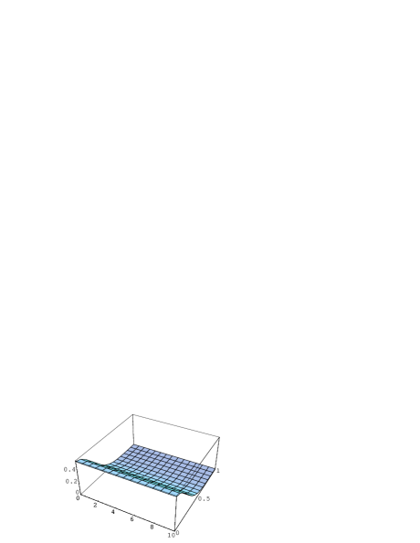
Figure 1: The flavorless density in the complex plane $\rho_{s}^{(0)}(\xi)$ at $\alpha^{2}=0.2$ (left) and the microscopic density of real eigenvalues for $2N_{f}=2$ massless flavors (right).

With the general structure of the massive correlators being clear from eq. (3.11) we also give explicitly the massless two-flavor case:

$$\rho^{(4)}_{S}(\xi) = \frac{1}{\pi\alpha}\exp\left[-\frac{2}{\alpha^{2}}{\Im\mbox{m}}^{2}\xi\right]\left\{g_{\alpha}(2i{\Im\mbox{m}}\ \xi)\ -\ \frac{g_{\alpha}(\xi)g_{\alpha}(\xi^{\ast})}{g_{\alpha}(0)}\right.$$ (3.14)

$$\left.+\ \frac{\left(\sqrt{\frac{2}{\pi}}\mbox{e}^{-\alpha^{2}/2}\sin\xi-\xi g_{\alpha}(\xi)\right)\left(\sqrt{\frac{2}{\pi}}\mbox{e}^{-\alpha^{2}/2}\sin\xi^{\ast}-\xi^{\ast}g_{\alpha}(\xi^{\ast})\right)}{\left(\sqrt{\frac{2}{\pi}}\mbox{e}^{-\alpha^{2}/2}-g_{\alpha}(0)\right)}\right\}.$$

In contrast to the correlation functions of real eigenvalues [13] the massless correlation functions do not simplify here. The procedure of sending successively all masses to zero in eq. (3.11) leading to higher order derivatives of $g_{\alpha}$ will not simplify the determinant structure. The reason for this will become clear when comparing to the Hermitian limit below. Taking for example the microscopic density with $N_{f}$ massless flavors we will obtain a determinant of size $N_{f}+1$ even in the limit $\alpha\to 0$. It is only through non-trivial identities that this expression can be rewritten as a sum of bilinear combinations of half-integer Bessel-functions for an arbitrary Number $2N_{f}$ of massless flavors as first derived in [13].

3.1 The Hermitian limit

We will now discuss the Hermitian limit when $\alpha\to 0$. In the simplest case of zero flavors the microscopic density of the Hermitian matrix model is simply constant. For the complex density eq. (3.12) this feature is maintained on the real axis while the density smoothly spreads into the complex plane as depicted in Fig. 1 (left) (see also [30]). Taking the limit $\alpha\to 0$ of eq. (3.12) we obtain a delta-function times a constant, the density of the real eigenvalues:

$$\lim_{\alpha\to 0}\rho_{S}^{(0)}(\xi)\ =\ \frac{1}{\sqrt{\pi}}\delta\left(\sqrt{2}{\Im\mbox{m}}\ \xi\right)\lim_{\alpha\to 0}g_{\alpha}(2i{\Im\mbox{m}}\ \xi)\ =\ \nu(0)\delta\left({\Im\mbox{m}}\ \xi\right)\ ,$$ (3.15)

where in the last step we have used $\lim_{\alpha\to 0}g_{\alpha}(0)=\sqrt{2\pi}\nu(0)$. If we unfold the microscopic density as $\rho_{S}(\xi)=\lim_{N\to\infty}DR_{N}(D\xi)$ with respect to the full mean level spacing, $D=1/(\pi\nu(0)N)$, we obtain the parameter free result $\rho_{S}^{(0)}(\xi)=1/\pi$ [13]. Next, we turn to $2N_{f}=2$ where we take the massless limit for simplicity. In the Hermitian model the density is given by [13]

$$\rho_{S}^{(2)}(\xi)\ =\ \frac{1}{\pi}\left(1-\frac{\sin^{2}(\xi)}{\xi^{2}}\right)\ ,\ \ \ \ \xi\ \in{\mathbf{R}}\ \ ,$$ (3.16)

Figure 2: The microscopic density in the complex plane $\rho_{s}^{(2)}(\xi)$ of $2N_{f}=2$ massless flavors for different values of $\alpha^{2}=0.5$ (left) and $\alpha^{2}=0.1$ (right).

which is plotted in Fig. 1 (right). The corresponding density in the complex plane, eq. (3.13) with $\mu=0$, is plotted in Fig. 2 for two different values of $\alpha$. It very nicely combines both properties of Fig. 1, the oscillations of eq. (3.16) on the real axis (right) and the same spreading into the complex plane (left) of eq. (3.12) for $N_{f}=0$. For decreasing $\alpha$ the distribution gets narrower, slowly approaching the delta-function. This is also the reason for the different normalization in Figs. 1 and 2 for different values of $\alpha$. More mathematically we obtain from eq. (3.13)

$$\lim_{\alpha\to 0}\rho_{S}^{(2)}(\xi)\ =\ \nu(0)\delta({\Im\mbox{m}}\ \xi)\left(1-\frac{\sin^{2}(\pi\nu(0)\xi)}{(\pi\nu(0)\xi)^{2}}\right)\ .$$ (3.17)

When unfolding with respect to the mean level spacing $D$ we thus recover eq. (3.16).

Let us now turn to the Hermitian limit in the general case. For that purpose we first consider the Hermitian limit of the zero-flavor Kernel eq. (3.6) as a building block. We obtain [9]

$$\lim_{\alpha\to 0}K_{S}^{(0)}(\xi_{1},\xi_{2}^{\ast})\ =\ \nu(0)\sqrt{2}\ \delta\left(\sqrt{{\Im\mbox{m}}^{2}\xi_{1}+{\Im\mbox{m}}^{2}\xi_{2}}\right)\frac{\sin(\pi\nu(0)(\xi_{1}-\xi_{2}^{\ast}))}{\pi\nu(0)(\xi_{1}-\xi_{2}^{\ast})}\ .$$ (3.18)

After unfolding with respect to $D$ instead of $1/N$ this becomes precisely the parameter free universal sine-kernel of [32] on the real axis. It therefore does not come as a surprise that we also recover the known result for the microscopic massive $k$-point correlations

$$\lim_{\alpha\to 0}\rho^{(2N_{f})}_{S}(\xi_{1},\ldots,\xi_{k}) = \nu(0)^{k}\prod_{i=1}^{k}\delta\left({\Im\mbox{m}}\ \xi_{i}\right)$$ (3.26)

$$\times\frac{{\begin{array}[]{c}\det\\ \mbox{{\footnotesize$1\leq j,l\leq k$}}\\ \mbox{{\footnotesize$1\leq f,h\leq N_{f}$}}\end{array}}\left[\begin{array}[]{ll}\displaystyle\frac{\sin(\pi\nu(0)(\xi_{j}-\xi_{l}))}{\pi\nu(0)(\xi_{j}-\xi_{l})}&\displaystyle\frac{\sin(\pi\nu(0)(\xi_{j}+i\mu_{h}))}{\pi\nu(0)(\xi_{j}+i\mu_{h})}\\ &\\ \displaystyle\frac{\sin(\pi\nu(0)(i\mu_{f}-\xi_{l}))}{\pi\nu(0)(i\mu_{f}-\xi_{l})}&\displaystyle\frac{\sinh(\pi\nu(0)(\mu_{f}+\mu_{h}))}{\pi\nu(0)(\mu_{f}+\mu_{h})}\end{array}\right]}{\det_{1\leq f,h\leq N_{f}}\left[\displaystyle\frac{\sinh(\pi\nu(0)(\mu_{f}+\mu_{h}))}{\pi\nu(0)(\mu_{f}+\mu_{h})}\right]}\ .$$

Taken in units of $D$ it exactly coincides with the corresponding result for the Hermitian model as derived in [21] from the underlying field theory. The equivalence with the original form [18] can be shown using consistency conditions on QCD₃ finite volume partition functions [31].

Let us come back to the remark at the end of section 2. Had we taken the partition function eq. (2.2) for real eigenvalues in the beginning, together with a general polynomial in the exponential of the weight function eq. (2.3), we would have immediately arrived at eq. (3.26) after employing eq. (2.12) and the zero-flavor kernel eq. (3.18). We therefore rederive the results of [18] without any effort. The universality of our results then follows from that of the sine-kernel [32, 19].

3.2 Universality

Up to now we have only discussed a large-$N$ limit in which the eigenvalues are rescaled with the mean level spacing, the microscopic limit. When we want to discuss the issue of universality we have to distinguish another type of large-$N$ limit, the macroscopic limit. In this limit the short range fluctuations typically of the order $1/N$ are smoothed and the macroscopic (or smoothed or wide) correlation functions are obtained. Technically speaking the large-$N$ limit is taken without a rescaling (or unfolding) of the eigenvalues. This limit is also meaningful since here universal correlation functions can be obtained [33] as well. An example for such a macroscopic correlation function is the density in eq. (3.3), the smoothed eigenvalue density of the real part of the eigenvalues. For all three Gaussian ensembles of real eigenvalues it is given by the Wigner semi-circle. However, for a measure including terms of higher order than Gaussian the macroscopic spectral density $\nu(x)$ itself is non-universal as it explicitly includes all parameters of the higher order terms.

Going back to complex correlation functions the authors of [25] have shown a certain degree of universality for the macroscopic spectral density $\rho(x,y)$, with $z=x+iy$, in the limit of weak non-Hermiticity. Using supersymmetry they have shown that it only depends on the real part $x$ trough the combination $\nu(x)$, eq. (3.3). Hence the macroscopic density as a function of $y$ only, denoted by $\rho_{x}(y)$ in [25], is universal in the sense that when the scale is set by fixing the real part of the eigenvalues as $x=X$ in [25] or $x=0$ as in our case of origin scaling, $\nu(x)$ plays the role of a universal parameter in the case of a non-Gaussian weight function. Similar results have been obtained in [4] for weakly non-symmetric real matrices.

A more interesting point is the universality of the fluctuations in the microscopic correlations we have calculated in eq. (3.11). We have shown that given the flavorless correlations determined in [9] are universal their universality would automatically carry over to our massive results trough eq. (2.12) in the microscopic limit. From the derivation [25] of the kernel eq. (3.4) it is obvious, that the occurrence of the mean spectral density of the real eigenvalues $\nu(X)$ inside the integral eq. (3.4) is strictly related to the form of the measure eq. (2.3). We can therefore only conjecture that the kernels eq. (3.4) and (3.6) and thus the corresponding correlations are universal also for a more general weight than eq. (2.3). However, we can offer a non-trivial check in the Hermitian limit $\alpha\to 0$. As we have seen in this limit the flavorless kernel eq. (3.4) maps to the sine-kernel eq. (3.18) which is guaranteed to be universal [32, 19]. In the microscopic origin scaling limit the universal parameter $\nu(0)$ occurs in the correct place after taking the limit $\alpha\to 0$ of eq. (3.6). The same argument thus holds for the Hermitian limit eq. (3.26) of eq. (3.11). It would be highly desirable to repeat the universality proof of [19] for orthogonal polynomials in the complex plane in order to obtain eq. (3.6) and consequently eq. (3.11) for an for an arbitrary weight function.

For a very recent discussion of universality of complex spectra from the point of view of the Fokker-Planck equation we refer to [34].

3.3 Discussion of $\alpha$ as a function of $\mu_{chem}$

As it has been discussed already in the introduction the naive introduction of a chemical potential by writing the Dirac operator as $H+i\mu_{chem}$ does not lead to nontrivial correlations of complex eigenvalues. It either lead to a complete quenching or, after rescaling with keeping $N\mu_{chem}$ fixed, to a constant shift in the eigenvalues. We therefore have introduced a truly complex Dirac operator $J$ and we would like to understand the role of the parameter $\alpha$ governing the non-Hermiticity as a function of chemical potential $\mu_{chem}$. It would be therefore very instructive to compare to the RMT model in four dimensions [6] and identify the parameters. However, in QCD₄ much less is known. Only the macroscopic density and its support are known [6] as a functions of $\mu_{chem}$ in the RMT model while the microscopic correlations to be compared with lattice simulations are still lacking.

What we can do is to calculate the variation of the imaginary part of the eigenvalues, ${\Im\mbox{m}}\ \xi$, in the limit $\alpha\to 0$ and compare it to a vanishing potential $\mu_{chem}\to 0$ in [6]. For simplicity let us consider the zero-flavor case with microscopic density eq. (3.12). We can calculate the second moment along the imaginary axis $<{\Im\mbox{m}}^{2}\xi>\equiv\int_{-\infty}^{\infty}\!d{\Im\mbox{m}}\xi\ {\Im\mbox{m}}^{2}\xi\ \rho_{S}^{(0)}(\xi)$ given by

$$<{\Im\mbox{m}}^{2}\xi>\ =\ \frac{1}{4\pi}\alpha^{2}\left(1+\frac{2}{3}\alpha^{2}\right).$$ (3.27)

On the QCD₄ side we can ask with which power of $\mu_{chem}$ the unscaled imaginary part of the eigenvalues vanishes on the boundary of the support. It follows from [6] that

$${\Im\mbox{m}}\ z\ =\ \mu_{chem}^{2}\sqrt{4-{\Re\mbox{e}}^{2}z}\ +\ {\cal O}(\mu_{chem}^{4})\ .$$ (3.28)

We notice that the mean spectral density $\nu(x)$ naturally occurs. It is therefore tempting to identify at least to lowest order

$$\alpha(\mu_{chem})\ \sim\ \mu_{chem}^{2}\ .$$ (3.29)

Of course we do not have to make this identification. We could also simply take $\alpha$ as a fit parameter to compare with numerical data for the QCD₃ Dirac operator with chemical potential once they are available. The analytical form of the microscopic correlations would still be fixed by eq. (3.11).

Let us mention a direct application for QCD₄ with chemical potential. It has been found empirically that also away from the origin the bulk correlations of Dirac operator eigenvalues can be very well described by RMT [14] (for the most precise tests we refer to [15]). In the bulk of the spectrum the Dirac determinant and thus the chiral properties are no longer seen which makes our non-chiral RMT eq. (2.2) applicable. Thus we can take the zero-flavor microscopic correlation function of complex eigenvalues eq. (3.9) to test QCD₄ correlation functions with chemical potential in the bulk of the spectrum. As it was shown in [6] the macroscopic spectral density in the complex plane is independent of the real part ${\Re\mbox{e}}\ z$ of the eigenvalues. This is consistent with the quenched microscopic density eq. (3.12). One could thus check if the complex eigenvalues decay microscopically as depicted in Fig. 1 (left) along a fixed line of of constant ${\Re\mbox{e}}\ z$ parallel to the real axis. Comparing for different values of $\mu_{chem}$ would then fix the constant $\alpha$ as a function of $\mu_{chem}$. We stress that also the higher order correlation functions are available analytically in eq. (3.9). The corresponding real correlations eq. (3.26) have been already tested in [15] for vanishing chemical potential.

4 Microscopic limit II: strong non-Hermiticity

In this section we treat the large-$N$ limit in which the parameter $\tau$, or more specifically the combination $\sqrt{(1-\tau)/(1+\tau)}$ in the definition (2.4) is kept fixed. Here, there will be no limit possible to recover the correlations of the original Hermitian model and thus QCD₃ with real eigenvalues, such as discussed in subsection 3.1. However, we will find nontrivial generalizations of the original work of Ginibre [10]. It turns out, that when introducing quark flavors the microscopic spectral density starts to decay compared to the zero-flavor case, where it is entirely flat on the support [10] (see eq. (4.3)).

The major difference to the weak non-Hermitian limit comes from the fact that the mean level spacing is changed to be $D\sim 1/\sqrt{N}$. When looking at the weight function eq. (2.3) with $1-\tau$ fixed we can define the microscopic origin scaling limit for strong non-Hermiticity as

$$\sqrt{N}({\Re\mbox{e}}\ z+i{\Im\mbox{m}}\ z)\ =\ \sqrt{N}z\ \equiv\ \xi\ \ \ ,\ \sqrt{N}m_{f}\ \equiv\ \mu_{f}\ .$$ (4.1)

The microscopic kernel which is now defined as $K_{S}(\xi_{1},\xi_{2}^{\ast})=K_{N}(\xi_{1}/\sqrt{N},\xi_{2}^{\ast}/\sqrt{N})/\sqrt{N}$ can be directly obtained for $N_{f}=0$ by taking the limit (4.1) of the result for finite-$N$, eq. (2.13) [25]:

$$K_{S}^{(0)}(\xi_{1},\xi_{2}^{\ast})\ =\ \frac{1}{\pi(1-\tau^{2})}\exp\left[\frac{1}{2(1-\tau^{2})}\left(2\xi_{1}\xi^{\ast}_{2}-|\xi_{1}|^{2}-|\xi_{2}|^{2}+\frac{\tau}{2}({\xi^{\ast}_{1}}^{2}-\xi_{1}^{2}+\xi_{2}^{2}-{\xi^{\ast}_{2}}^{2})\right)\right]\ .$$ (4.2)

At equal arguments we thus obtain a constant microscopic density for zero flavors [10, 25]

$$\rho^{(0)}_{S}(\xi)\ =\ \frac{1}{\pi(1-\tau^{2})}\ .$$ (4.3)

It coincides with the smoothed or macroscopic spectral density of the unscaled eigenvalues [10] which has been reobtained in [25] using the supersymmetric method

$$\rho(z)\ =\ \lim_{N\to\infty}\frac{1}{N}R_{N}(z)\ =\ \left\{\begin{array}[]{cl}\displaystyle\frac{1}{\pi(1-\tau^{2})}\ ,&\displaystyle\ \ \mbox{if}\ \ \frac{{\Re\mbox{e}}^{2}z}{(1+\tau)^{2}}+\frac{{\Im\mbox{m}}^{2}z}{(1-\tau)^{2}}\leq 1\\ \displaystyle 0\ ,&\displaystyle\ \ \mbox{otherwise}\end{array}\ .\right.$$ (4.4)

The latter is independent of the number of quarks present as it is obtained from saddle point analysis where the quark determinants are subleading. We recall that in the RMT of QCD₄ [6] the support of the macroscopic density is as well given by an algebraic curve and, although not being flat, the density is independent of the real part of the Dirac operator eigenvalues.

Next we turn to the microscopic correlation functions in the presence of $2N_{f}$ massive quarks. Inserting the zero-flavor kernel eq. (4.2) into eq. (3.10) now in the strong non-Hermitian limit eq. (4.1) we obtain for the general $k$-point function

$$\rho^{(2N_{f})}_{S}(\xi_{1},\ldots,\xi_{k})=\left(\frac{1}{\pi(1-\tau^{2})}\right)^{k}\prod_{i=1}^{k}\exp\left[\frac{-|\xi_{i}|^{2}}{1-\tau^{2}}\right]\frac{{\begin{array}[]{c}\det\\ \mbox{{\footnotesize$1\leq j,l\leq k$}}\\ \mbox{{\footnotesize$1\leq f,h\leq N_{f}$}}\end{array}}\left[\begin{array}[]{ll}\displaystyle\exp\left[\frac{\xi_{j}\ \xi_{l}^{\ast}}{1-\tau^{2}}\right]&\displaystyle\exp\left[\frac{-\xi_{j}\ i\mu_{h}}{1-\tau^{2}}\right]\\ &\\ \displaystyle\exp\left[\frac{i\mu_{f}\ \xi_{l}^{\ast}}{1-\tau^{2}}\right]&\displaystyle\exp\left[\frac{\mu_{f}\ \mu_{h}}{1-\tau^{2}}\right]\\ \end{array}\right]}{\det_{1\leq f,h\leq N_{f}}\left[\displaystyle\exp\left[\frac{\mu_{f}\ \mu_{h}}{1-\tau^{2}}\right]\right]}.$$ (4.5)

Here, we have taken those parts in eq. (4.2) which factorize out of the determinant, leading to a partial cancelation. Let us explicitly display the simplest examples, the density with one massive flavor

$$\rho^{(2)}_{S}(\xi)\ =\ \frac{1}{\pi(1-\tau^{2})}\left\{1\ -\ \exp\left[-\frac{1}{1-\tau^{2}}|\xi-i\mu|^{2}\right]\right\}\ ,$$ (4.6)

and the density with two massless flavors

$$\rho^{(4)}_{S}(\xi)\ =\ \frac{1}{\pi(1-\tau^{2})}\left\{1\ -\ \left(1+\frac{|\xi|^{2}}{1-\tau^{2}}\right)\exp\left[-\frac{|\xi|^{2}}{1-\tau^{2}}\right]\right\}\ .$$ (4.7)

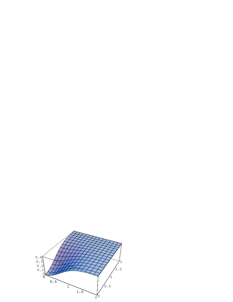
Figure 3: The massless microscopic density in the complex plane $\rho_{s}^{(2N_{f})}(\xi)$ for $2N_{f}=2$ (left) and $2N_{f}=4$ (right), both at $\tau=1/2$.

In both cases it is no longer constant. For vanishing masses both vanish at the origin $\xi=0$ due to the level repulsion of the additional quark flavors. For large arguments they both approach the value of the macroscopic density eq. (4.4). As we can see in Fig. 3 for two flavors (right) the level repulsion is stronger.

We finally note that the microscopic correlations in the limit of strong non-Hermiticity can be obtained from those in the weak limit by taking $\alpha\to\infty$, as being mentioned already in [25]. In this limit eq. (4.5) follows from eq. (3.11) when identifying $\alpha^{2}\equiv(1-\tau^{2})$. In the simplest example eq. (3.12) leads to the constant density eq. (4.3). We thus find a crossover from the regime of weak to strong non-Hermiticity with growing $\alpha$. A similar crossover has been seen for the nearest neighbor distribution in quenched QCD₄ lattice data [11] as a function of growing $\mu_{chem}$.

5 Conclusions

We have derived analytic expressions for all correlation functions of complex Dirac operator eigenvalues in the presence of an arbitrary even number of massive quark flavors. Here, we have replaced the Dirac operator for QCD₃ by a general complex matrix as we have argued that a shift of an originally Hermitian operator by a constant chemical potential, $i\mu_{chem}$, would not lead to non-trivial correlations. We have solved the problem in the limit of weak and strong non-Hermiticity and have identified the parameter for non-Hermiticity $\alpha$ as modeling the influence of a chemical potential. Our results may also be useful for QCD lattice data with chemical potential in four dimensions in the bulk of the spectrum. In the limit of a Hermitian Dirac operator we could nicely reproduce the known results for real eigenvalues. Moreover, we could offer a very elegant alternative of calculating massive real eigenvalue correlations and proving their RMT universality.

There are several open questions we have not addressed so far. The main task is a generalization of our results to chiral RMT as an effective model for QCD₄ spectra close to the origin. The crucial step would be to find the corresponding orthogonal polynomials in the complex plane to make our techniques applicable. An open problem within our calculations is the question of universality of the correlation functions which we could only conjecture. The problem is to show that for an arbitrary weight function we will obtain orthogonal polynomials with the same asymptotic as the Hermite polynomials. Given the success for real eigenvalues in this respect progress should be possible. Another question is to find the finite-volume partition function corresponding to the partition function of complex eigenvalues. In other words one would have to find an appropriate unitary group integral given by the determinant of the massive kernel of complex eigenvalues.

Another open problem would be the generalization to the other invariant random matrix ensembles, the orthogonal and symplectic ensemble, to incorporate complex eigenvalues. First results have been obtained only for the macroscopic spectral density of almost symmetric matrices using the supersymmetric method.

Acknowledgments
I wish to thank S. Pepin for useful discussions and reading the manuscript. This work was supported in part by EU TMR grant no. ERBFMRXCT97-0122.

References

- [1] N. Hatano and D.R. Nelson, Phys. Rev. Lett. 77 (1996) 570-573 [cond-mat/9603165].
- [2] F. Haake, Quantum Signatures of Chaos, Springer Verlag, Berlin 1991.
- [3] R. Grobe, F. Haake and H.-J. Sommers, Phys. Rev. Lett. 61 (1988) 1899-1902.
- [4] K.B. Efetov, Phys. Rev. Lett. 79 (1997) 491-494 [cond-mat/9702091].
- [5] Y.V. Fyodorov and B.A. Khoruzhenko, Phys. Rev. Lett. 83 (1999) 65-68 [cond-mat/9903043].
- [6] M.A. Stephanov, Phys. Rev. Lett. 76 (1996) 4472-4475 [hep-th/9604003].
-
[7]
S. Chandrasekharan, Nucl. Phys. Proc. Suppl. 94
(2001) 71-78 [hep-lat/0011022];
F. Karsch, Nucl. Phys. Proc. Suppl. 83 (2000) 14-23 [hep-lat/9909006]. - [8] J.J.M. Verbaarschot and T. Wettig, Ann. Rev. Nucl. Part. Sci. 50 (2000) 343-410 [hep-ph/0003017].
- [9] Y.V. Fyodorov, B.A. Khoruzhenko and H.-J. Sommers, Phys. Rev. Lett. 79 (1997) 557-561 [cond-mat/9703152].
- [10] J. Ginibre, J. Math. Phys. 6 (1965) 440-449.
- [11] H. Markum, R. Pullirsch and T. Wettig, Phys. Rev. Lett. 83 (1999) 484-487 [hep-lat/9906020].
- [12] R.A. Janik, M.A. Nowak, G. Papp and I. Zahed, Phys. Rev. Lett. 81 (1998) 264-267 [hep-ph/9803289].
- [13] J.J.M. Verbaarschot and I. Zahed, Phys. Rev. Lett. 73 (1994) 2288-2291 [hep-th/9405005].
- [14] M.A. Halàsz and J.J.M. Verbaarschot, Phys. Rev. Lett. 74 (1995) 3920-3923 [hep-lat/9501025].
- [15] T. Guhr, J.-Z. Ma, S. Meyer and T. Wilke, Phys. Rev. D59 (1999) 054501 [hep-lat/9806003].
- [16] P.H. Damgaard, U.M. Heller, A. Krasnitz and T. Madsen, Phys. Lett. B440 (1998) 129-135 [hep-lat/9803012].
-
[17]
B. Vanderheyden and A.D. Jackson,
Phys. Rev. D62 (2000) 094010 [hep-ph/0003150];
S. Pepin and A. Schäfer, Eur. Phys. J. A10 (2001) 303-308 [hep-ph/0010225]. - [18] P.H. Damgaard and S. Nishigaki, Phys. Rev. D57 (1998) 5299-5302 [hep-th/9711096].
- [19] G. Akemann, P.H. Damgaard, U. Magnea and S. Nishigaki, Nucl. Phys. B487 (1997) 721-738 [hep-th/9609174].
-
[20]
G. Akemann and P.H. Damgaard, Nucl.
Phys. B528 (1998) 411-431 [hep-th/9801133];
J. Christiansen, Nucl. Phys. B547 (1999) 329-342 [hep-th/9809194]. - [21] R. Szabo, Nucl. Phys. B598 (2001) 309-347 [hep-th/0009237].
- [22] G. Akemann, P.H. Damgaard, D. Dalmazi and J.J.M. Verbaarschot, Nucl. Phys. B601 (2001) 77-124 [hep-th/0011072].
- [23] D. Dalmazi and J.J.M. Verbaarschot, hep-th/0101035.
- [24] G. Akemann and G. Vernizzi, Nucl. Phys. B583 (2000) 739-757 [hep-th/0002148].
- [25] Y.V. Fyodorov, B.A. Khoruzhenko and H.-J. Sommers, Ann. Inst. Henri Poincaré 68 (1998) 449-489 [chao-dyn/9802025].
- [26] P. Di Francesco, M. Gaudin, C. Itzykson and F. Lesage, Int. J. Mod. Phys. A9 (1994) 4257-4351.
- [27] M.L. Mehta, Random Matrices, Academic Press, London 1991.
- [28] G. Szegö, Orthogonal Polynomials, American Mathematical Society, Providence RI 1939.
- [29] G. Akemann and E. Kanzieper, Phys. Rev. Lett. 85 (2000) 1174-1177 [hep-th/0001188].
- [30] Y.V. Fyodorov, B.A. Khoruzhenko and H.-J. Sommers, Phys. Lett. A226 (1997) 46-52 [cond-mat/9606173].
- [31] G. Akemann and P.H. Damgaard, Phys. Lett. B432 (1998) 390-396 [hep-th/9802174].
- [32] E. Brézin and A. Zee, Nucl. Phys. B402 (1993) 613-627.
- [33] J. Ambjørn, J. Jurkiewicz and Yu. Makeenko, Phys. Lett. B251 (1990) 517-527.
- [34] P. Shukla, cond-mat/0105007.