HUTP-01/A026

HU-EP-01/22

hep-th/0106040

Open/Closed String Dualities and Seiberg Duality

from Geometric Transitions in M-theory

Keshav Dasgupta ^a,, Kyungho Oh^b, and Radu Tatar^c,

^a School of Natural Sciences, Institute for Advanced Study, Princeton NJ 08540, USA

^b Lyman Laboratory of Physics, Harvard University, Cambridge, MA 02138, USA

^c Institut fur Physik, Humboldt University, Berlin, 10115, Germany

Abstract

We propose a general method to study open/closed string dualities from transitions in M theory which is valid for a large class of geometrical configurations. By T-duality we can transform geometrically engineered configurations into ${\cal N}=1$ brane configurations and study the transitions of the corresponding branes by lifting the configurations to M-theory. We describe the transformed degenerated M5 branes and extract the field theory information on gluino condensation by factorization of the Seiberg-Witten curve. We also include massive flavors and orientifolds and discuss Seiberg duality which appears in this case as a birational flop. After the transition, the Seiberg duality becomes an abelian electric-magnetic duality.

June 2001

1 Introduction

Beginning with Maldacena’s AdS/CFT conjecture [1], the duality between gauge theories and gravity has been actively studied by using the open/closed string theory dualities, mainly on non-compact singular or compact Calabi-Yau $n$-folds. Geometric engineering and ‘brane engineering’ are two of the main useful techniques.

Geometric engineering [2, 3] is a very powerful tool, but sometimes it is hard to manipulate due to rigid holomorphic structures. On the other hand, brane configurations, typically in the flat geometric background, are relatively easy to manipulate and, by utilizing Witten’s MQCD methods [25, 26], it has been very successfully used in studying the non-perturbative dynamics of low energy supersymmetric gauge theories.

Often T duality has been applied to go from the geometric set-up to the brane configuration set-up (with NS branes and D branes) [4] but the results were obtained for semi-localized configurations where the NS branes were smeared on some compact directions. In this paper, we systematically utilize T duality and Witten’s MQCD [25, 26] to investigate the ${\cal N}=1$ large N duality proposed by Vafa [6, 7]. Because we consider the T-dualities given by a ${\bf C}^{*}$ action on smooth Calabi-Yau spaces, our solutions are fully localized, although we do not write explicit supergravity solutions. The NS branes are fully localized because their directions are identified with some fixed lines in the geometry, as we will see in the detailed discussion of the T-duality. The smooth Calabi-Yau spaces considered here are either versal deformations or Kähler deformations of singular Calabi-Yau spaces with only conifold singularities.

Recently, using previous results on Chern-Simons/topological strings duality [5], Vafa suggested a dual picture in the large N limit between open string theory on D-branes wrapped over the ${\bf P}^{1}$ cycle of a resolved conifold and a closed string theory on the deformed conifold where the D-branes have disappeared and have been replaced by RR fluxes through the ${\bf S}^{3}$ cycle, together with NS fluxes through the dual noncompact 3-cycle [6]. The conifolds have been studied extensively in the last years in view of AdS/CFT duality and they play a role in understanding dynamics of ${\cal N}=1$ supersymmetric theories [21].

The solution has been generalized to more complicated non-compact geometries in [10, 7, 16]. The ten dimensional transition appears as a geometric flop in M theory on a $G_{2}$ holonomy manifold [9, 8, 14]. The question is whether the transition in more complicated geometries as the ones of [10, 7, 16] (and some other geometries build in the same way) can be lifted to flops in other $G_{2}$ holonomy manifolds. The known non-compact examples are sparce [12, 13] . It would be nice to find an alternative method to study the transition from D-branes wrapped on 2-cycles of some geometry to fluxes through 3-cycles of some other geometrical set-up.

Such an alternative method was proposed by us in [22] where we considered Vafa’s transition by using the MQCD brane configurations [25, 26]. We started with $U(N)$ gauge group given by $N$ D5 branes wrapped on the ${\bf P}^{1}$ cycle of a resolved conifold. Under a T-duality on the circle action of the resolved conifold gives a brane configuration with $N$ D4 branes between two orthogonal NS5 branes. By lifting to M theory, this becomes a single M5 brane which includes the Seiberg-Witten curve for $SU(N)$ theory, the $U(1)$ part of $U(N)$ being, in general, decoupled. In our discussion, a crucial point was that for $N$ D5 branes wrapped on ${\bf P}^{1}$ cycle of a resolved conifold, in the limit when the cycle is of very small size, there is a transition from the $U(N)$ theories on the branes to $U(1)$ theory on the bulk. In this limit, the Seiberg-Witten curve degenerates and it describes a $U(1)$ theory. The component $\Sigma$ of the M5 brane becomes a “plane M5 brane”. The coupling constant of the $U(1)$ gauge group has a RG flow which can be shown to arise naturally from the cut-off applied to regulate a divergent integral over the period of the degenerated $\Sigma$. This cut-off in the integral is related to the UV cutoff of the dual gauge theory. Our results offer a check of the new point of view stated in [23] concerning the fact that that the Chern-Simons/topological strings duality of [5] is more natural for the $U(N)$ gauge group.

In [22], we provided a rederivation of results already obtained by using $G_{2}$ holonomy manifolds. One can ask whether the same method can be applied for more complicated geometries, where a $G_{2}$ holonomy manifold is not known. The answer is yes and this is the subject of our current paper. Our claim is that any geometry which resembles the conifold can be treated in the same way as the conifold itself. These geometries involve D5 branes wrapped on different ${\bf P}^{1}$ cycles which, after T-duality, give more complex brane configurations with orthogonal NS branes and D4 branes between them and which then can be lifted to a single M5 brane.

In the present paper we consider two such geometries. The first one is the geometry used in [7] for an ${\cal N}=2$ theory deformed by a superpotential with terms with different powers of the adjoint field and the second one is a geometry describing $U(N)$ group with fundamental matter. For the second geometry, we discuss the electric/magnetic Seiberg duality between $SU(N)$ and $SU(F-N)$ theories ($F$ being the number of flavors) and provide some hints for the product gauge groups. In the geometrical picture, the Seiberg duality appears as a flop transition, a fact which was suggested in [37, 7], and here we provide a proof of this.

In discussing the brane configurations which correspond to the geometry of [7], we study the transition between M5 branes corresponding to the product of $SU(N_{i})$ gauge groups and degenerate M5 branes corresponding to a product of $U(1)$ groups. We make a clear identification of the parameters of the M5 branes in terms of ${\cal N}=1$ field theoretical scales. These parameters are related to different fluxes in the geometrical side of the type IIB transition. The degenerate M5 brane describes the Seiberg-Witten reduced curve and its exact form is derived. Our result should be compared to the one in [7], where the match between the Seiberg-Witten reduced curve and the curve given by the period matrix of the geometry was checked only at the highest order.

We also discuss the case when we have orientifolds and the results of the M5 brane transition is to be compared with results of [10, 16].

2 Vafa’s ${\cal N}=1$ Duality and Brane Configurations

2.1 Large $N$ Duality Proposal

It has been proposed that there exists a open-closed string duality between field theories on D branes wrapped on ${\bf P}^{1}$ cycles and closed string theory on complex deformed Calabi-Yau manifolds [6]. In [7] it has been discussed that an ${\cal N}=1$, $U(N)$ theory with adjoint and superpotential

$$W_{tree}=\sum_{p=1}^{n+1}~{}{g_{p}\over p}{\mbox{Tr}}\Phi^{p}$$ (1)

(obtained on D5 branes wrapped on several 2-cycles of a resolved geometry) is dual to an $U(1)^{n}$ theory with superpotential

$$-{1\over 2\pi i}W_{eff}=\sum_{i=1}^{n}~{}(N_{i}\int_{B_{i}}^{\Lambda_{0}}~{}\Omega+\alpha_{i}\int_{A_{i}}~{}\Omega)$$ (2)

In the formulae (1) and (2), the variables $n$ and $g_{p}$ are given in terms of geometry of the Calabi-Yau, the quantities $N_{i}$ are the total $H_{R}$ fluxes through the $A_{i}$ cycles and $\alpha_{i}$ are $\tau H_{NSNS}$ fluxes through the $B_{i}$ cycles. This theory has a UV cutoff given by $\Lambda_{{\cal N}=1}\equiv\Lambda_{0}$ which we shall refer simply as $\Lambda$ henceforth.

Before going further we would like to make some comments on the existence of the $H_{NSNS}$ field. If we just consider the proposal that D5 branes wrapped on various ${\bf P}^{1}$ cycles disappear and are replaced by the supergravity background they create, then this would imply the existence of $H_{RR}$ only as the $H_{NSNS}$ field could be switched to zero. But this is not the case and we can give two arguments for this:

(1) Vafa’s original idea [6] in type IIA picture was based on a geometry whose complex structure was not integrable which implies the existence of a 4-form through the noncompact 4-cycle of a resolved conifold. This is the NS 4-form which goes into the mirror dual into an NS 3-form through the noncompact 3-cycle of a deformed conifold. Therefore, the NS 3-form has geometrical origin and cannot be switched off.

(2) In order to identify the geometrical cut-off with the scale of the gauge theory, we need the term $\frac{1}{g_{0}^{2}}S$ in the superpotential (where $g_{0}$ is the bare coupling constant) which comes from integrating the $H_{NSNS}$ over the noncompact 3-cycle. So $H_{NSNS}$ cannot be turned off.

2.2 Brane Construction and Geometric Transition

In the previous section we studied the duality conjecture from the point of view of special geometry. There is an alternative way to motivate this duality. And this is by using brane configurations. The conifold geometry can also be studied from intersecting brane constructions by making a T-duality and going to type IIA. Let us discuss this construction in some details since similar constructions will be used throughout the rest of the paper.

Consider an action $S_{c}$ on the conifold given by $xy-uv=0$ as:

$$S_{c}:~{}~{}(e^{i\theta},x)\to x,~{}~{}(e^{i\theta},y)\to y~{}~{}(e^{i\theta},u)\to e^{i\theta}u,~{}~{}(e^{i\theta},v)\to e^{-i\theta}v,~{}~{}$$ (3)

The orbits of the action $S_{c}$ degenerates along the union of two intersecting complex lines $y=u=v=0$ and $x=u=v=0$ on the conifold. This action can be lifted to the resolved conifold and deformed conifold. As discussed in [22], the T-dual picture for the D5 branes on the finite 2-cycle of the resolved conifold will be a brane configuration with D4 branes along the interval with two NS branes in the ‘orthogonal’ direction at the ends of the the interval, the length of the interval being the same as the size of the rigid ${\bf P}^{1}$ . For the deformed conifold, by taking the T-duality, we obtain an NS brane along the curve $u=v=0$ with non-compact direction in the Minkowski space which is given by

$$xy=\mu$$ (4)

in the x-y plane.

The above is thus the brane constructions for a conifold, resolved conifold and deformed conifold. Now to study Vafa’s duality we appeal to Witten’s MQCD construction [25, 26]. As we saw above, $N$ D5 branes wrapping a 2-cycle of a resolved conifold map to $N$ D4 branes between two orthogonal NS5 branes separated along $x^{7}$ directions. We denote the directions of the two NS5 branes along $x^{0,1,2,3,4,5}$ and $x^{0,1,2,3,8,9}$ respectively. The D4 branes are along $x^{0,1,2,3,7}$.

When we lift this configuration to M-theory all the branes in the picture become a single M5 brane with complicated world-volume structure. We define the complex coordinates:

$$x=x^{4}+ix^{5},~{}~{}~{}y=x^{8}+ix^{9},~{}~{}~{}t=exp(-R^{-1}x^{7}+ix^{10})$$ (5)

where $R$ is the radius of the $11th$ direction, the world volume of the M5 corresponding to the resolved conifold is given by $R^{1,3}\times\Sigma$ and $\Sigma$ is a complex curve defined, up to an undetermined constant $\zeta$, by

$$y=\zeta x^{-1},~{}~{}t=x^{N}$$ (6)

Now if we consider the limit where the size of ${\bf P}^{1}$ goes to zero, then the value of $t$ on $\Sigma$ must be constant because $\Sigma$ is holomorphic and there is no non-constant holomorphic map into ${\bf S}^{1}$. Therefore the M5 curve make a transition from a “space” curve into a “plane” curve. From (6), we obtain $N$ possible plane curves

$$\Sigma_{k}:~{}~{}~{}t=t_{0},~{}~{}xy=\zeta\exp{2\pi ik/N},\quad k=0,1,\ldots,N-1.$$ (7)

This is the way we see Vafa’s duality transformation. After the transition the degenerate M5 branes are no longer considered as the M-theory lift of D4 branes. This is now a closed string background, and in fact if one looks at the T-dual picture of the deformed conifold (4) then this is exactly the M-theory lift of the deformed conifold.

3 Large N Duality Proposal for ${\cal N}=1$ Theory with adjoint and superpotential

3.1 Geometric engineering and Brane configuration

In [7], the large N duality conjecture of Vafa [6] has been generalized to ${\cal N}=1$ $SU(N)$ theory with adjoint chiral superfield $\Phi$ and with tree-level superpotential

$${W_{\mbox{tree}}}=\sum_{k=1}^{n+1}\frac{g_{k}}{k}{\mbox{Tr}}\Phi^{k}$$ (8)

The classical theory with superpotential (8) has many vacua, where the eigenvalues of $\Phi$ are various roots of

$$W^{\prime}(x)=\sum_{k=1}^{n+1}\frac{g_{k}}{k}x^{k}\equiv g_{n+1}\prod_{k=1}^{n}(x-a_{k}).$$ (9)

In [22], the case for $n=1$ in ${W_{\mbox{tree}}}$ has been considered.

Without the superpotential (8), the theory is just four dimensional ${\cal N}=2$ Yang-Mills theory. This can be geometrically engineered on the total space of the normal bundle ${\cal O}(-2)+{\cal O}(0)$ over ${\bf P}^{1}$. The ${\cal N}=2$ $U(N)$ gauge theory is obtained on the world-volume of $N$ D5 branes wrapping the ${\bf P}^{1}$ [7]. The adjoint scalar $\Phi$ is identified with the deformations of the brane in the ${\cal O}(0)$ direction.

To describe the geometry in detail, we introduce two ${\bf C}^{3}$ whose coordinates are $Z,X,Y$ (resp. $Z^{\prime},X^{\prime},Y^{\prime}$) for the first (resp. second) ${\bf C}^{3}$. Then the total space of the normal bundle ${\cal O}(-2)+{\cal O}(0)$ over ${\bf P}^{1}$ is given by gluing two ${\bf C}^{3}$’s with the identification:

$$Z^{\prime}=1/Z,~{}~{}X^{\prime}=X,~{}~{}Y^{\prime}=YZ^{2}$$ (10)

Now we will introduce a circle action and take a T dual along the orbits of the circle action. Consider a circle action $S_{2}$:

$$(e^{i\theta},Z)=e^{i\theta}Z,~{}~{}(e^{i\theta},X)=X,~{}~{}(e^{i\theta},Y)=e^{-i\theta}Y$$ (11)

$$(e^{i\theta},Z^{\prime})=e^{-i\theta}Z^{\prime},~{}~{}(e^{i\theta},X^{\prime})=X^{\prime},~{}~{}(e^{i\theta},Y^{\prime})=e^{i\theta}Y^{\prime}$$

Note that the action $S_{2}$ is compatible with (10) so that it is defined on ${\cal O}(-2)+{\cal O}(0)$. Since the orbits of the action degenerate along $Z=Y=0$ and $Z^{\prime}=Y^{\prime}=0$, we have two NS branes along $X$ direction at $Z=Y=0$ and $Z^{\prime}=Y^{\prime}=0$ after T-duality. Now if we take the T-dual of $N$ D5 wrapping ${\bf P}^{1}$, it will be a brane configuration of $N$ D4 branes between two NS branes spaced along $X$ (Figure 1). Two NS branes are parallel because the $X$ is coordinate of the trivial bundle ${\cal O}(0)$ over ${\bf P}^{1}$.

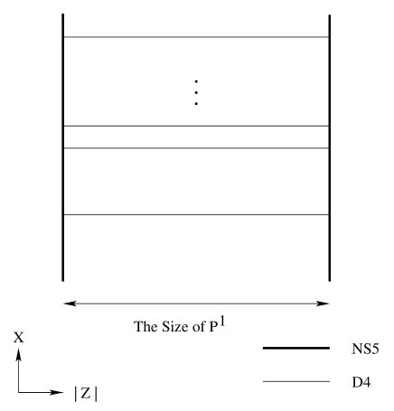
Figure 1: The T-dual configuration of $N$ D5 on ${\bf P}^{1}$ in ${\cal O}(-2)+{\cal O}(0)$ over ${\bf P}^{1}$.

The D4 branes can freely move along the direction of the NS branes corresponding to the direction in the Coulomb branch, and the position of D4 brane is identified with the eigenvalues of the adjoint field $\Phi$. This is ${\cal N}=2$ $U(N)$ theory.

By adding the superpotential ${W_{\mbox{tree}}}$ (8), the theory will be broken to ${\cal N}=1$ in which the NS brane is curved into the $y$-space from the straight line configuration in the ${\cal N}=2$ theory. We will only consider the case where all vacua are non-degenerate i.e. $W^{\prime}(X)$ has distinct roots. The T-dual of this ${\cal N}=1$ brane configuration can be geometrically engineered on a Calabi-Yau space. We consider a small resolution of a Calabi-Yau with conifold singularities:

$${\cal C}:~{}~{}y(y-W^{\prime}(x))-uv=0$$ (12)

where $W^{\prime}(x)=g_{n}\prod_{k=1}^{n}(x-a_{k})$ with distinct $a_{k}$. Note that the singular points are located at $y=W^{\prime}(x)=0$. It will be shown that the singularities can be resolved by successive blow-ups which replace each singular point by ${\bf P}^{1}$. The resolved space $\tilde{{\cal C}}$ can be covered by two copies of ${\bf C}^{3}$, $U_{p}$, $p=0,1$ with coordinates $Z,X,Y$ (resp. $Z^{\prime},X^{\prime},Y^{\prime}$) which are related by

$$Z^{\prime}=Z^{-1},\,\,X^{\prime}=X,\,\,Y^{\prime}=YZ^{2}-W^{\prime}(X)Z.$$ (13)

The resolution map $\sigma$ from the resolved space $\tilde{{\cal C}}$ to the singular Calabi-Yau space ${\cal C}$ is given by

$$x=X=X^{\prime},\,\,y=YZ=Y^{\prime}Z^{\prime}+W^{\prime}(X^{\prime}),\,\,$$ (14)

$$u=Y=Z^{\prime}(Y^{\prime}Z^{\prime}+W^{\prime}(X^{\prime})),\,\,v=Z(YZ-W^{\prime}(X))=Y^{\prime}$$ (15)

The geometry change from the ${\cal N}=2$ theory (10) to the ${\cal N}=1$ theory (13) shows that the ${\bf P}^{1}$ cycles in ${\cal N}=1$ theory are fixed at $x=a_{k}$, $k=1,\ldots,n$ (which are the roots of $W^{\prime}(x)=0$) while there is a family of ${\bf P}^{1}$ cycles in the ${\cal N}=2$ theory. Since the circle action $S_{2}$ (3.1) is compatible with the identification (10) for the ${\cal N}=1$ geometry, the T-duality can be taken along the direction of the orbits of the action $S_{2}$ on $\tilde{{\cal C}}$. The orbits degenerate along $Z=Y=0$ and $Z^{\prime}=Y^{\prime}=0$. Thus after T-duality, we have two NS branes which, under the resolution map $\sigma$, map to $y=u=v=0$ and $y=W^{\prime}(x),u=v=0$ on ${\cal C}$. Hence we obtain two NS branes, one straight NS brane denoted by NS and one curved NS brane denoted by NS^′ and the supersymmetry is broken to ${\cal N}=1$. On the other hand, D5 branes along ${\bf P}^{1}$ cycles become D4 branes after T-duality. If we distribute the $N$ D5 branes among the vacua $a_{k}$ by wrapping $N_{k}$ branes on the ${\bf P}^{1}$ at $x=a_{k}$, this breaks the gauge group:

$$U(N)\to U(N_{1})\times\cdots\times U(N_{n}).$$ (16)

We obtain a brane configuration with two non-parallel NS branes and D4 branes between them as shown in (Figure 2) after T-duality. In the limit $g_{n}\to\infty$, the curved NS brane will be broken into $n$ NS branes (Figure 3).

Figure 2: The T-dual configuration of $N$ D5 distributed among $n$ ${\bf P}^{1}$.

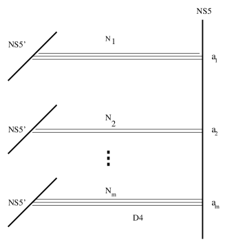
Figure 3: The brane configuration in the limit $g_{n}\to\infty$.

In [7], the large N duality has been proposed via the geometric transition from the small resolution $\tilde{{\cal C}}$ of ${\cal C}$ to a complex deformation of ${\cal C}$. As we have $n$ isolated conifold singular points, the complex deformation space (i.e. versal deformation space) is $n$ dimensional whose parameters are given as $\mu_{1},\ldots,\mu_{n}$. This can be obtained by adding a polynomial $f_{n-1}(x,\mu_{1},...\mu_{n})$ of degree $n-1$ in $x$ with $f_{n-1}(a_{k},\mu_{1},\ldots,\mu_{n})=\mu_{k}$ to (12), which is given by

$$f_{n-1}(x,\mu_{1},...\mu_{n})=\sum_{k=1}^{n}\mu_{k}\ \prod_{l=1,l\neq k}^{n}\frac{x-a_{l}}{a_{k}-a_{l}}.$$ (17)

Hence the deformed generalized conifold is given by

$${\cal C}_{s}:~{}~{}W^{\prime}(x)y-f_{n-1}(x,\mu_{1},\ldots,\mu_{n})-uv=0.$$ (18)

The equation (18) defines a variety in ${\bf C}^{n}\times{\bf C}^{4}$ where the coordinates of ${\bf C}^{n}$ are $\mu_{1},\ldots,\mu_{n}$ and the smoothing $\Delta$ is given by the map induced by the natural projection:

$$\Delta:{\cal C}_{s}\to{\bf C}^{n}$$ (19)

and the fiber over the origin is the original singular Calabi-Yau space ${\cal C}$ (12). On the generic fiber $\Delta^{-1}(\mu_{1},\ldots,\mu_{n})$, the $n$ three sphere ${\bf S}^{3}$ of size $\mu_{k}$ will smooth out the singular point $x=a_{k},y=u=v=0$. We consider a circle action ${\cal S}_{d}$ on (18) by

$$({e^{i\theta}},x)\to x,~{}~{}({e^{i\theta}},y)\to y,~{}~{}({e^{i\theta}}u)\to{e^{i\theta}}u,~{}~{}({e^{i\theta}}v)\to{e^{-i\theta}}v.$$ (20)

Now if we take T dual along the orbits of the action ${\cal S}_{d}$, then NS brane will appear along $u=v=0$ which is given by

$$W^{\prime}(x)y=f_{n-1}(x,\mu_{1},\ldots,\mu_{n}).$$ (21)

3.2 M theory interpretation

In MQCD [26], the classical type IIA brane configuration turns into a single fivebrane whose world-volume is a product of the Minkowski space ${\bf R}^{1,3}$ and a complex curve in a flat Calabi-Yau manifold

$$M={\bf C}^{2}\times{\bf C}^{*}.$$ (22)

We denote the finite direction of D4 branes by $x^{7}$ and the angular coordinate of the circle ${\bf S}^{1}$ in the 11-th dimension by $x^{10}$. Thus the NS branes are separated along the $x^{7}$ direction. We combine them into a complex coordinate

$$t=\exp(-R^{-1}x^{7}-ix^{10})$$ (23)

where $R$ is the radius of the circle ${\bf S}^{1}$ in the 11-th direction.

Let us review the construction of the complex curve $\Sigma$ in the case of two orthogonal NS branes with $N$ D4 branes between them. On $\Sigma$ the coordinates of NS branes goes to the infinity only at their locations. So we may identify $\Sigma$ with a punctured complex plane with coordinate $x$, and since there are $N$ D4 branes in the type IIA picture, we should have $t=x^{N}$. Hence the $\Sigma\subset M$ is an embedding of the punctured $x$ plane ${\bf C}^{*}$ into the Calabi-Yau space $M$ by the map

$${\bf C}^{*}\longrightarrow\Sigma\subset M,~{}~{}~{}~{}~{}x\to(x,\zeta x^{-1},x^{N})$$ (24)

The brane configuration of the generalized conifold consists of $(n+1)$ NS branes with $N_{k}$ D4 branes between the first and $(k+1)$-th NS branes. Hence the $\Sigma$ in this case will be an embedding of $n$-punctured complex plane, coordinatized by $x$, into the Calabi-Yau space $M$. The $x$ coordinates of the punctures are given by $a_{k}$ which is the location of the NS branes. Since there are $N_{k}$ D4 branes between the first and $(k+1)$-th NS branes, we should have $t=(x-a_{k})^{N_{k}}$ around $x=a_{k}$. Thus the $\Sigma\subset M$ is an embedding of the $n$-punctured $x$ plane into the Calabi-Yau space $M$ by the map

$${\bf C}-\{a_{1},\ldots,a_{k}\}\longrightarrow\Sigma\subset M,~{}~{}~{}~{}~{}x\to(x,~{}\sum_{k=1}^{n}\frac{\zeta_{k}}{x-a_{k}},~{}~{}\prod_{k=1}^{n}(x-a_{k})^{N_{k}}).$$ (25)

There are $(n+1)$ components at infinity and the bending behavior is as follows:

$$x\to\infty,~{}~{}y\to 0,~{}~{}~{}~{}t\sim x^{N_{1}+\cdots+N_{n}}$$ (26)

$$x\to a_{k},~{}~{}y\to\infty,~{}~{}~{}~{}t\sim\zeta_{k}^{N_{k}}\prod_{i=1,i\neq k}^{n}(a_{k}-a_{i})^{N_{i}}y^{-N_{k}}.$$

We would like to identify the parameters $\zeta_{k}$ of (25) in terms of the scales of the ${\cal N}=1$ field theory. We begin with the ${\cal N}=2,U(N)$ curve which is

$$t^{2}+B(x,u_{k}))t+\Lambda_{{\cal N}=2}^{2N}=0$$ (27)

where we restored a dimensional dependence on the QCD scale $\Lambda_{{\cal N}=2}^{2N}$. We need to deform this curve to (25) which describes ${\cal N}=1$ $U(N_{1})\times\cdots\times U(N_{n})$ supersymmetric gauge theory. We first consider a degeneration of (27) to the form

$$t^{2}+t\prod_{k=1}^{n}(x-a_{k})^{N_{k}}+\Lambda_{{\cal N}=2}^{2N}=0.$$ (28)

In the classical type IIA limit, this corresponds to a brane configuration of two parallel NS branes and $n$ groups of $N_{k}$ coincident D4 branes located at $x=a_{1},\ldots a_{n}$ between two NS branes. There are $N$ such points in the Coulomb branch and each of them are related by the discrete group ${\bf Z}_{2N_{1}}\times\cdots\times{\bf Z}_{2N_{n}}$ in which each factor acts on the QCD scale as

$$\Lambda_{{\cal N}=2}^{2}\rightarrow e^{2\pi i/N_{k}}\Lambda_{{\cal N}=2}^{2}.$$ (29)

For $t\to\infty$, the degenerate curve (28) is asymptotically $t\sim x^{N}$ and to see the asymptotic behavior for $t\to 0$ and $x\to a_{k}$, we rewrite (28) as

$$\frac{t}{\prod_{i=1,i\neq k}^{n}(x-a_{i})^{N_{i}}}+(x-a_{k})^{N_{k}}+\frac{\Lambda_{{\cal N}=2}^{2N}}{t\prod_{i=1,i\neq k}^{n}(x-a_{i})^{N_{i}}}=0.$$ (30)

As $t\to 0$ and $x\to a_{k}$, the degenerate curve (30) is asymptotically

$$x-a_{k}\sim\frac{\Lambda_{{\cal N}=2}^{2N/N_{k}}}{t^{1/N_{k}}\prod_{i=1,i\neq k}^{n}(a_{k}-a_{i})^{N_{i}/N_{k}}}$$ (31)

At large $t$ we have a curve approaching $x=t^{1/N}$ and $y$ is small, while for $t\rightarrow 0$ the curve approaches $y_{k}=\mu_{k}x$ for the $k$-th NS^′ brane where $\mu_{k}$ is the mass of the $SU(N_{k})$ adjoint. For the deformation (8), the mass of the $SU(N_{k})$ adjoint field is

$$\mu_{k}=g_{n+1}\prod_{i\neq k}(a_{k}-a_{i})$$ (32)

so

$$y_{k}=g_{n+1}\Lambda_{{\cal N}=2}^{2N/N_{i}}\prod_{i\neq k}(a_{k}-a_{i})^{1-N_{i}/N_{k}}t^{-1/N_{k}}$$ (33)

By threshold matching between the high energy $SU(N)$ theory with the low energy theory obtained by integrating out the adjoint fields and the massive W bosons, one obtains:

$$\Lambda_{k}^{3}=g_{n+1}\Lambda_{{\cal N}=2}^{2N/N_{i}}\prod_{i\neq k}(a_{k}-a_{i})^{1-2N_{i}/N_{k}}$$ (34)

where $\Lambda_{k}$ is the scale of the low-energy $SU(N_{k})$ theory. From (33) and (34), we can rewrite $y_{k}$ as:

$$y_{k}=\Lambda_{k}^{3}\prod_{i\neq k}(a_{k}-a_{i})^{N_{i}/N_{k}}t^{-1/N_{k}}$$ (35)

We can now compare the equations (35) and (26). The boundary condition for $x\rightarrow a_{k}$ is

$$y_{k}=\zeta_{k}\prod_{i\neq k}(a_{k}-a_{i})^{N_{i}/N_{k}}t^{-1/N_{k}}$$ (36)

We then see that $\zeta_{k}=\Lambda_{k}^{3}$ which, as we would expect, looks the same as for the $SU(N)$ case.

If we now consider the fivebrane (25), we see that its asymptotics depend on $\zeta_{i}^{N_{i}}$ but the brane itself depends on $\zeta_{i}$, so the M5 branes related by the $Z_{N_{1}}\times\cdots\times Z_{N_{n}}$ transformations:

$$\zeta_{i}\rightarrow e^{\frac{2\pi i}{N_{i}}}\zeta_{i},~{}~{}~{}~{}i=1,~{}\cdots,~{}n$$ (37)

have the same asymptotic behavior but differ in shape. Therefore the $N_{i}$ possible value for each $\zeta_{i}$ corresponds to a different M5 brane and hence to a different vacuum of the quantum theory. We shall see below that these different quantum states split after we go through a transition. The fact that the curve (25) has properties which are just a simple generalization of the $SU(N)$ case makes it easier to give a description of confinement.

When the size of ${\bf P}^{1}$ goes to zero, the $x^{7}$ direction in the M-theory will be very small and negligible. The modulus of $t$ on $\Sigma$ will be fixed i.e. $\Sigma$ will be a curve in the cylinder ${\bf S}^{1}\times{\bf C}^{2}$ where ${\bf S}^{1}$ is the circle in the 11-th dimension and ${\bf C}^{2}$ are coordinatized by $x,y$. In fact, the value of $t$ on $\Sigma$ must be constant because $\Sigma$ is holomorphic and there is no non-constant holomorphic map into ${\bf S}^{1}$. The M5 curve makes a transition from a space curve into a plane curve. We now need to eliminate $t$ since the dimension of $t$ on $\Sigma$ is virtually zero and the information along $t$ is not reliable. In the process of eliminating $t$, there are $N_{k}$ possibilities of $\zeta_{k}$ since only $\zeta_{k}^{N_{k}}$, and not $\zeta_{k}$, enters in the behavior at infinity. They represent possible supersymmetric vacua in the gauge theory which is determined by the interior behavior of the brane. Thus we obtain the following relation between $x$ and $y$:

$$yW^{\prime}(x)=\sum_{k=1}^{n}\zeta_{k}\exp(2\pi im_{k,i}/N_{k})\prod_{l=1,l\neq k}(x-a_{l}),$$ (38)

where $m_{k}=1,\ldots,N_{k}$ for $k=1,\ldots,n$. Since this is the limit where $g_{s}N$ is big, this degenerate M5 brane should not be considered as a M theory lift of D branes. In this limit, the metrically deformed background without the D-branes is the right description and this is a closed string geometric background.

The T dual picture of the deformed conifold (18) is exactly an M theory lift of the NS brane of the deformed conifold with

$$\mu_{k}=\zeta_{k}\exp(2\pi im_{k,i}/N_{k})\prod_{l=1,l\neq k}(a_{k}-a_{l}).$$ (39)

The size of ${\bf S}^{3}$ on the deformed conifold depends on the expectation value for the gluino condensation and, for each value of the gluino condensate we will have different flux through the ${\bf S}^{3}$ cycle. We may intuitively consider the plane M5 as one obtained from two intersecting M5 branes by smearing out the intersection point due to the flux from the vanished D4 branes wrapped on ${\bf P}^{1}$.

3.3 Field theory analysis

The ${\cal N}=2$ pure $SU(N)$ Yang-Mills theory can be obtained by wrapping N D5 branes on the zero section of ${\cal O}(-2)+{\cal O}(0)$ over ${\bf P}^{1}$. After taking T-duality along the direction of the circle action ${\cal S}_{2}$ of (3.1) and lifting to M-theory, we obtain M5 curve of the form:

$$t^{2}+B(x)t+1=0$$ (40)

where

$$B(x)=x^{N}+u_{1}x^{N-1}+u_{2}x^{N-2}+\ldots+u_{k}$$ (41)

(for $SU(N)$ we impose $u_{1}=0$). The deformation of the theory by the superpotential ${W_{\mbox{tree}}}$ has been achieved by perturbing the geometry from ${\cal O}(-2)+{\cal O}(0)$ over ${\bf P}^{1}$ to a Calabi-Yau with $n$ ${\bf P}^{1}$’s with normal bundle ${\cal O}(-1)+{\cal O}(-1)$ which are located at $x=a_{1},\ldots,x_{n}$. In the T-dual type IIA picture, we have one NS branes and $n$ NS^′ branes (Figure 2) and the NS^′ branes are located at $x=a_{1},\ldots,x_{k}$. Hence classically we have

$$yW^{\prime}(x)=1$$ (42)

where $y$ is the coordinates of NS^′ and $x$ is that of NS. The gauge group $U(N)$ is broken into $U(N_{1})\times\cdots\times U(N_{n})$, and after gluino condensations, the final gauge theory is ${\cal N}=1$ $U(1)^{n}$ theory. The $k$-th $U(1)$ gauge field of $U(1)^{n}$ theory is given by the center of the mass coordinates of $N_{k}$ D4 branes along the NS branes. Since the $N_{k}$ branes are coincident in the type IIA picture, the moduli of $U(1)^{n}$ is classically described by the NS branes which is given by

$$yW^{\prime}(x)=1.$$ (43)

But if we lift the branes configuration to the M-theory, the quantum effects will show up and the corresponding M5 brane is given by an embedding of the $n$-punctured $x$ plane into the Calabi-Yau space $M$ by the map

$${\bf C}-\{a_{1},\ldots,a_{k}\}\longrightarrow\Sigma\subset M,~{}~{}~{}~{}~{}x\to(x,~{}\sum_{k=1}^{n}\frac{\zeta_{k}}{x-a_{k}},~{}~{}g_{n}\prod_{k=1}^{n}(x-a_{k})^{N_{k}}).$$ (44)

Hence the MQCD moduli of the $U(1)^{n}$ is given by

$$yW^{\prime}(x)=f_{n-1}(x,\zeta_{1},\ldots,\zeta_{n}),$$ (45)

which is the M-theory description of the NS branes. Here $f_{n-1}(x,\zeta_{1},\ldots,\zeta_{n})$ is given as in (17). As we have discussed in [22], the effective low energy four dimensional theory comes from the world volume of the M5 brane and the low effective action is determined by the Jacobian of the M5 brane. Since (45) is a non-compact curve which is a ${\bf P}^{1}$ with $(n+1)$ points punctured, the Jacobian is an algebraic group $({\bf C}^{*})^{*}$ and

$$H^{1}(({\bf C}^{*})^{n},{\bf Z})=\oplus_{k=1}^{n}{\bf C}\frac{dx}{x-a_{k}}.$$ (46)

By putting the cut-off at $|x|=\Lambda_{0,k}^{3/2}$, the integral over the $k$-th component of the Jacobian $({\bf C}^{*})^{n}$

$$\int_{{\bf C}^{*}}d\log x\wedge\ast d\log x\sim 3\log\Lambda_{0,k}-\log|\zeta_{k}|$$ (47)

becomes finite and the coupling constants of the $k$-th component of $U(1)^{n}$ is given by

$$\frac{1}{g_{k}^{2}}\sim 3\log\Lambda_{0,k}-\log|\zeta_{k}|$$ (48)

which is the expected running of the coupling constant if we replace the cutoff $\Lambda_{0,k}$ by the scale of the gauge theory $\Lambda_{k}$.

On the other hand, the ${\cal N}=2$ pure $SU(N)$ Yang-Mills theory deformed by a tree level superpotential (8) only has unbroken supersymmetry on submanifolds of the Coulomb branch, where there are additional massless fields besides the $u_{k}$. They are nothing but the magnetic monopoles or dyons which become massless on some particular submanifolds $\langle u_{k}\rangle$ where the Seiberg–Witten curve degenerates. Near a point with $l$ massless monopoles, the superpotential is

$$W=\sqrt{2}\sum_{i=1}^{l}M_{i}A_{i}\tilde{M}_{i}+\sum_{k=1}^{n+1}g_{k}U_{k}~{},$$ (49)

where $A_{i}$ are the chiral superfield parts of the $U(1)$ vector multiplet corresponding to an ${\cal N}=2$ dyon hypermultiplet $M_{i}$ and $U_{k}$ are the chiral superfields representing the operators ${\mbox{Tr}}(\Phi^{k})$ in the low energy theory. The vevs of the lowest components of $A_{i},M_{i},U_{k}$ are written as $a_{i},m_{i},u_{k}$. The supersymmetric vacua are at those $\langle u_{k}\rangle$ satisfying:

$$a_{i}(\langle u_{k}\rangle)=0~{},~{}~{}~{}~{}~{}~{}~{}g_{k}+\sqrt{2}\sum_{i=1}^{l}\frac{\partial a_{i}}{\partial u_{k}}(\langle u_{k}\rangle)m_{i}\tilde{m}_{i}=0~{},$$ (50)

for $k=1,\ldots,n+1$. The value of the superpotential at this vacuum is given by

$${W_{\mbox{eff}}}=\sum_{k=1}^{n+1}g_{k}\langle u_{k}\rangle~{}.$$ (51)

Recall that the Seiberg-Witten curve of ${\cal N}=2$ $U(N)$ is

$$y^{2}=P(x;u_{r})^{2}-4\Lambda^{2N}_{{\cal N}=2},P(x,u_{r})\equiv\det(x-\Phi)=\sum_{k=0}^{N}x^{N-k}s_{k}$$ (52)

where the $s_{k}$ are related to the $u_{r}$ by the Newton’s formula

$$ks_{k}+\sum_{r=1}^{k}ru_{r}s_{k-r}=0,$$ (53)

and $s_{0}\equiv 1$ and $u_{0}\equiv 0$. The condition for having $N-n$ mutually local massless magnetic monopoles is that

$$P_{N}(x,\langle u_{p}\rangle)^{2}-4\Lambda^{2N}_{{\cal N}=2}=(H_{N-n}(x))^{2}F_{2n}(x)$$ (54)

where $H_{N-n}$ is a polynomial in $x$ of degree $N-n$ with distinct roots and $F_{2n}$ is a polynomial in $x$ of degree $2n$ with distinct roots.

On the $n$ massless photons, the one corresponding to the trace of $U(N)$, does not couple to the rest of the theory and so its coupling constant is the one we started with. The other $n-1$ photons which are left massless after the breaking $U(N)\to U(N_{1})\times\cdots\times U(N_{n})$ have gauge couplings which are given by the period matrix of the reduced curve

$$y^{2}=F_{2n}(x;\langle u_{r}\rangle)=F_{2n}(x;g_{k},\Lambda)$$ (55)

with $F_{2n}(x;\langle u_{k}\rangle)$ the same functions appearing in (54) and $\langle u_{r}\rangle$ the point of the solution space of (54) which minimize ${W_{\mbox{tree}}}$. The curve (55) thus gives the exact gauge couplings of $U(1)^{n-1}$ which remains massless in (50) as function of $g_{k}$ and $\Lambda$.

Comparing the results from the MQCD, the curve (55) cannot be isomorphic to the curve (45) because, for $n>1$, the curve (55) is hyperelliptic while the curve (45) is rational. But two curves are intimately related. We may rewrite (55) as

$$y^{2}=W^{\prime}(x)\left(W^{\prime}(x)+\frac{f_{n-1}(x)}{W^{\prime}(x)}\right).$$ (56)

From this form, it is clear that one can obtain (45) from (55) and vice versa in a canonical way. Thus the moduli (55) and (45) are equivalent. This also can be traced back to the fact that our model is based on the singular conifold whose equation is given by

$$W^{\prime}(x)y-uv=0.$$ (57)

If we now replace the above equation by

$$W^{\prime}(x)^{2}+y^{2}-uv=0,$$ (58)

we obtain the same model and after the transition the geometric background for the closed string will be given by

$$W^{\prime}(x)^{2}+f_{n-1}+y^{2}-uv=0$$ (59)

which is the original form given in [7]. Via T-duality, the geometric background is given as an NS brane wrapping on

$$W^{\prime}(x)^{2}+f_{n-1}(x)+y^{2}=0.$$ (60)

Thus the moduli will be described by

$$W^{\prime}(x)^{2}+f_{n-1}(x)+y^{2}=0,$$ (61)

and we can prove two curves (55) and (61) are isomorphic i.e.

$$W^{\prime}(x)^{2}+f_{n-1}(x)=-g^{2}_{n+1}F_{2n}(x)$$ (62)

after possible coordinates changes. This was proved up to a certain order of $x$ in [7]. But we do not expect to have a proof via M-theory because the M5 curve for ${\cal N}=1$ is always rational. It is a hyperelliptic curve only in the case of ${\cal N}=2$. The moduli (55) looks like a ${\cal N}=2$ curve in a sense that the curve is a plane curve rather than a space curve which is also reflected by the fact that we have massive glueballs.

4 Adding Matter Fields and Orientifold Planes

We can add some quark chiral superfields in the fundamental representation of $U(N_{k})$ for $k=1,\ldots,n$ generalizing the discussion of [7]. In the type IIB, the matter fields are added as D5 branes wrapping a holomorphic 2-cycle separated by a distance $m$ from the exceptional ${\bf P}^{1}$. There are two kinds of matter fields we may add. In the T-dual type IIA picture, the matter fields are obtained by adding semi-infinite D4 branes which can be attached either the NS brane or the NS^′ branes in the Figure 2. Recall that the small resolution $\tilde{{\cal C}}$ is covered by two copies of ${\bf C}^{3}$, $U_{p},p=0,1$ with coordiantes $Z,X,Y$ (resp. $Z^{\prime},X^{\prime},Y^{\prime}$). The semi-infinite D4 branes attached to the NS brane near the vacua $x=a_{k}$ is given by the D5 branes wrapping non-compact holomorphic cycles

$$Y=0,~{}~{}X-a_{k}=m_{k,1},\ldots,m_{k,F_{k}}.,$$ (63)

We can also put the semi-infinite D4 branes near $x=a_{k}$ attached to the NS^′ brane which are given by the D5 branes wrapping a non-compact holomorphic 2-cycles

$$Y^{\prime}=0,~{}~{}X^{\prime}-a_{k}=n_{k,1},\ldots,n_{k,G_{k}}.$$ (64)

These semi-infinite D4 branes give rise to $N_{k,f}$ hypermultiplets in the fundamental representation of $U(N_{k})$ corresponding to strings stretched between the $N_{k}$ D5 branes wrapping the exceptional ${\bf P}^{1}$ at $x=a_{k}$ and the $N_{k,f}$ non-compact D5 branes wrapping the holomorphic 2 cycles given by (63) and (64) and the mass is the distance between the non-compact D5 brane and the compact D5 wrapping ${\bf P}^{1}$. Thus we can geometrically engineer the ${\cal N}=1$ $U(N_{1})\times\cdots\times U(N_{n})$ theory with adjoints and $N_{k,f}$ hypermultiplets with mass $m_{k,1},\ldots,m_{k,N_{k,f}}$.

We remark that the distance between non-compact holomorphic 2-cycles defined (63) (resp. (64)) asymptotically approach to a fixed cycle. To see the asymptotic behavior of the cycles defined by (63), consider its defining equations in the open set $U_{1}$:

$$X^{\prime}-a_{k}=m_{k,1},\ldots,m_{k,F_{k}},Y^{\prime}=-W^{\prime}(a_{k}+m_{k,1})Z^{\prime-1},\ldots,-W^{\prime}(a_{k}+m_{k,F_{k}})Z^{\prime-1}.$$ (65)

Hence as ${\bf Z}\to\infty$ all cycles approaches to a cycle given by

$$X^{\prime}-a_{k}=m_{k,1},\ldots,m_{k,F_{k}},~{}~{}Y^{\prime}=0,$$ (66)

and thus there is no transversal oscillation at infinity. In the type IIA picture, they begin from NS brane at one side and tangentially approach to the other NS brane. So beyond a cut-off $|Z|=\Lambda_{0}$, the oscillations in the transversal direction can be ignored and the strings between them see only 4 infinite directions. This is important when we discuss the Seiberg duality and we impose the condition that in the magnetic picture the mesons live in a four dimensional theory. The same aspect was discussed in [30] where additional NS branes were needed in order to make the flavor D4 branes very long but finite. In [24] a similar consideration has been utilized in calculating the contribution of massive flavor to the superpotential.

We can also discuss the $SO/Sp$ theories by introducing additional orientifolds in the theory. The orientifolding can be introduced by extending the complex conjugation on the conifold defined by

$$z_{1}^{2}+z_{2}^{2}+z_{3}^{2}+z_{4}^{2}=0$$ (67)

to both complex and Kähler deformations. On the complex deformed conifold $T^{*}{\bf S}^{3}$, the special Lagrangian ${\bf S}^{3}$ is invariant under this complex conjugation and hence the orientifold is an O6 plane wrapping ${\bf S}^{3}$ [10, 13]. In MQCD, the theory with the superpotential can be obtained by rotating the NS branes as in [38].

We discuss now the type IIB picture by first reviewing the results of [16]. We shall concentrate on the case ${\cal N}=1,SO(N)$ gauge theory with matter $\Phi$ in the adjoint representation of $SO(N)$ and with the superpotential

$$W_{SO,tree}(\Phi)=\sum_{k=1}^{n+1}\frac{g_{2k}}{2k}Tr\Phi^{2k}$$ (68)

The classical theory with the superpotential (68) has vacua where the eigenvalues of $\Phi$ are roots of

$$W^{\prime}(x)=g_{n+1}x\prod_{j=1}^{n}(x^{2}+a_{j}^{2}),~{}~{}~{}a_{j}~{}>~{}0$$ (69)

In [16], we considered D5 on ${\bf P}^{1}$ cycles located at the zeros of $W^{\prime}(x)$. In the presence of an orbifold plane located at $x=0$, the ${\bf P}^{1}$ cycle at $x=0$ becomes an ${\bf RP}^{2}$ cycle stuck on the orientifold plane and the field theory on the D5 branes wrapped on it is $O(2N_{0})$. The D5 branes on ${\bf P}^{1}$ cycles located at $i~{}a_{j}$ are identified with the D5 branes on ${\bf P}^{1}$ cycles located at $-i~{}a_{j}$ and the field theory on the corresponding D5 branes is $U(N_{j})$, so the breaking of the gauge group is

$$O(N)\rightarrow O(N_{0})\times U(N_{1})\times\cdots\times U(N_{n})$$ (70)

If we blow down the geometry, it becomes a Calabi-Yau with conifold singularities (as in $SU(N)$ case), and we consider a small resolution of it as in (12). We take the action of the circle action ${\cal S}_{c}$ on $\tilde{{\cal C}}_{SO}$, where $\tilde{{\cal C}}_{SO}$ is the small resolution for the $SO$ case and the same arguments of section 3.1 tell us that the T-dual picture is a brane configuration with one $NS_{x}$ brane and $2(n+1)$ $NS_{Y^{\prime}_{i}},i=0,\cdots,2~{}n~{}+1$ located at $x=0,x=\pm ia_{j},j=1,\cdots n$, $N_{i},i=1,~{}\cdots,~{}2~{}n~{}+~{}1$ D4 branes connecting the $NS_{x}$ brane with an $NS_{Y^{\prime}_{i}}$ brane and $N_{0}$ D4 branes connecting the $NS_{x}$ brane with the $NS_{Y^{\prime}_{0}}$ brane. Under the orientifold action, the pairs of $NS_{Y^{\prime}_{i}}$ branes located at $\pm ia_{j},j=1,\cdots n$ are identified and give the $U(N_{1})\times\cdots\times U(N_{n})$ group and the D4 branes which connect the $NS_{x}$ with $NS_{Y^{\prime}_{0}}$ brane and stay on top of the orientifold plane give $O(N_{0})$ group.

We can also lift the configuration to M theory. The complex curve $\Sigma$ is the embedding of the complex plane coordinatized by $x$ and punctured at $0,~{}\pm ia_{i},i=1,\cdots,N$ into the Calabi-Yau space M by the map:

$${\bf C}-\{0,\pm ia_{1},\cdots,\pm ia_{n}\}\rightarrow\Sigma\subset M,~{}~{}~{}~{}~{}~{}x\rightarrow\left(x,\frac{\zeta_{0}}{x}+\sum_{k=1}^{n}\frac{\zeta_{k}}{x^{2}+a_{i}^{2}},\prod_{k=1}^{n}(x^{2}+a_{k}^{2})^{N_{k}}\right)$$ (71)

We could again identify the parameters $\zeta$ of the above curve with parameters of field theory by studying a degeneration of the Seiberg-Witten curve.

By considering now the limit when the size of the ${\bf P}^{1}$ cycle goes to zero, the M5 brane curve makes the transition from a space curve into a plane curve. which is the M theory lift of the NS brane of the orbifolded deformed conifold:

$$\mu_{k}=\zeta_{k}\exp(2\pi im_{k,i}/N_{k})\prod_{l=1,l\neq k}(a_{k}^{2}~{}-~{}a_{l}^{2})$$ (72)

for the ${\bf S}^{3}$ cycles which do not sit at the origin and

$$\mu_{0}=\zeta_{0}\exp(2\pi im_{0,i}/(N_{0}/2\pm 1))\prod_{l=1}a_{l}^{2}$$ (73)

for the $S^{3}$ cycle which sits at the origin. The values of $mu$ parameters appear in the plane M5 brane defining equations and are connected to the fluxes over the ${\bf S}^{3}$ cycles in type IIB picture.

The field theory analysis goes as in section 3.3.

5 Seiberg Duality versus Abelian Duality

5.1 $SU(N)$ group with $F$ flavors

We discuss now the well known Seiberg duality [28] in our framework. This states that the infrared behavior of $SU(N)$ theories with $F$ flavors of quarks $Q_{+}$ and antiquarks $Q_{-}$ have a dual description in terms of an $SU(\tilde{N})$ gauge group, $\tilde{N}=F-N$, with F flavors of quarks $\tilde{Q_{+}}$ and antiquarks $\tilde{Q_{-}}$, with gauge-singlet mesons $M\equiv Q_{+}Q_{-}$. The dual effective theory for massive quarks $Q$ (with equal mass $m$, for simplicity) has a superpotential

$$W_{\mbox{dual}}=\mbox{tr}~{}mM+\frac{1}{\mu}\tilde{Q_{+}}M~{}\tilde{Q_{-}}$$ (74)

and the strong interaction scale of the dual theory is

$$\tilde{\Lambda}^{3\tilde{N}-F}\Lambda^{3N-F}=(-1)^{\tilde{N}}\mu^{F}$$ (75)

where the scale $\mu$ appears in order to compensate the difference in dimension of the scales, and also the meson fields between the original and dual theories.

We will show that the Seiberg duality can be achieved by a birational flop in the the geometric engineering. To make it more clear, we first recall the flop process [31]. The conifold

$${\cal C}:~{}~{}xy-uv=0$$ (76)

have two small resolutions which will be denoted by ${\cal C}_{x}$ and ${\cal C}_{y}$:

$\bullet$ The small resolution ${\cal C}_{x}$

Let ${\bf C}^{3}_{0}$ and ${\bf C}^{3}_{\infty}$ be two ${\bf C}^{3}$ whose coordinates are $Z_{1},X_{1},Y_{1}$ and $Z^{\prime}_{1},X^{\prime}_{1},Y^{\prime}_{1}$ with identification:

$$Z^{\prime}_{1}=1/Z_{1},~{}~{}X^{\prime}_{1}=X_{1}Z_{1},~{}~{}Y^{\prime}_{1}=Y_{1}Z_{1}.$$ (77)

The blowing down map is given by

$$\sigma_{x}: {\cal C}_{x}={\bf C}^{3}_{0}\cup{\bf C}^{3}_{\infty}\longrightarrow{\cal C}$$

$$x=X_{1},~{}~{}y=Y_{1}Z_{1},~{}~{}u=Y_{1},~{}~{}v=X_{1}Z_{1}$$

$$x=X^{\prime}_{1}Z^{\prime}_{1},~{}~{}y=Y^{\prime}_{1},~{}~{}u=Y^{\prime}_{1}Z^{\prime}_{1},~{}~{}v=X^{\prime}_{1}.$$

$\bullet$ The small resolution ${\cal C}_{y}$

Let ${\bf C}^{3}_{0}$ and ${\bf C}^{3}_{\infty}$ be two ${\bf C}^{3}$ whose coordinates are $Z_{2},X_{2},Y_{2}$ and $Z^{\prime}_{2},X^{\prime}_{2},Y^{\prime}_{2}$ with identification:

$$Z^{\prime}_{2}=1/Z_{2},~{}~{}X^{\prime}_{2}=X_{2}Z_{2},~{}~{}Y^{\prime}_{2}=Y_{2}Z_{2}.$$ (79)

The blowing down map is given by

$$\sigma_{y}: {\cal C}_{y}={\bf C}^{3}_{0}\cup{\bf C}^{3}_{\infty}\longrightarrow{\cal C}$$

$$x=X_{2}Z_{2},~{}~{}y=Y_{2},~{}~{}u=X_{2},~{}~{}v=Y_{2}Z_{2}$$

$$x=X^{\prime}_{2},~{}~{}y=Y^{\prime}_{2}Z^{\prime}_{2},~{}~{}u=X^{\prime}_{2}Z^{\prime}_{2},~{}~{}v=Y^{\prime}_{2}.$$

The exchange of the role of $x$ and $y$ in the resolution induces an isomorphism $f:{\cal C}_{x}\to{\cal C}_{y}$ given by:

$$Z_{1}\mapsto Z_{2},~{}X_{1}\mapsto Y_{2}~{}Y_{1}\mapsto X_{2},~{}Z^{\prime}_{1}\mapsto Z^{\prime}_{2},~{}X^{\prime}_{1}\mapsto Y^{\prime}_{2},~{}Y^{\prime}_{1}\mapsto X^{\prime}_{2}.$$ (81)

We may define the circle action on $u,v$ variables as before. In the T-dual picture along the direction of the orbits of the circle action, the flop will take the $N_{x}$ (resp. $N_{y}$) brane (which is spaced along the $x$ (resp $y$)-direction) of ${\cal C}_{x}$ to the $N_{y}$ (resp. $N_{x}$) brane (which is spaced along the $y$ (resp. $x$)-direction) of ${\cal C}_{y}$. Nevertheless, it seems to be impossible to argue the Seiberg duality in the geometric engineering or in the brane set-up without going to the M-theory.

In the previous section we have discussed the realization in geometry for $SU(N)$ with fundamental matter. This is realized by having $N$ D5 branes wrapped on the exceptional ${\bf P}^{1}$ cycles and $F$ D5 branes wrapped on the 2-cycle (63),which gives by T-duality a brane configuration with two ‘orthogonal’ NS branes, together with $N$ D4 branes between them on an interval and $F$ semi-infinite D4 branes attached to one of the NS branes. The positions of the semi-infinite D4 branes on the NS branes determine the bare masses of the quark fields. This classical string theory brane configuration can be lifted to M5 curve $\Sigma$ as an embedding of the punctured $x$ plane into the Calabi-Yau space $M$:

$$x~{}\to~{}\left(x,~{}\zeta x^{-1},~{}\xi\frac{x^{N}}{\prod_{i=1}^{F}(x-m_{i})}\right)$$ (82)

where the parameters $\xi$ and $\zeta$ are identified with

$$\xi=(\prod_{i}m_{i})^{(F-N)/F}~{},~{}~{}\zeta=\Lambda^{(3N-F)/N}(\prod_{i}m_{i})^{1/N}.$$ (83)

Now the birational flop will change the role of $x$ and $y$, and hence the same M5 curve $\Sigma$ can be considered as an embedding of the punctured $y$ plane into the Calabi-Yau $M$ [29, 30]:

$$y~{}\to~{}\left(\tilde{\zeta}y^{-1},~{}y,~{}\tilde{\xi}(-1)^{F}\frac{y^{\tilde{N}}}{\prod_{i=1}^{F}(y-\langle M\rangle_{i}))}\right)$$ (84)

where the eigenvalues of the meson fields are given by

$$\langle M\rangle_{i}=\frac{(\prod_{i}m_{i})^{1/N}\Lambda^{(3N-F)/N}}{m_{i}},$$ (85)

and the new parameters are where

$$\tilde{\xi}~{}=~{}(\prod_{i}\langle M\rangle_{i})^{{F-\tilde{N}}/F},~{}~{}\tilde{\zeta}~{}=~{}(\prod_{i}\langle M\rangle_{i})^{1/{\tilde{N}}}\tilde{\Lambda}^{(3~{}\tilde{N}-F)/\tilde{N}}.$$ (86)

Here the new set of parameters are introduced in order to have field theory interpretation. Going from (82) to (84) means to go between the two sides of the Seiberg duality. Therefore, the birational flop induces the Seiberg duality. This M theory transition has been noticed in [29, 30].

We can now discuss of what happens in the limit of very small size of the ${\bf P}^{1}$ cycles where the $N$ D5 branes corresponding to color gauge group are wrapped. In this limit the value of t on $\Sigma$ is again a constant and both curved M5 branes (82),(84) have a transition to plane M5 branes as discussed in [22]. For the electric theory, in order to obtain the description of the plane M5 curves in this case, we first fix $t$ at $t_{0}$ and the equation (82) becomes:

$$t_{0}=\xi\frac{x^{N}}{\prod_{i=1}^{F}(x-m_{i})},t_{0}^{-1}=\zeta^{-N}\xi^{-1}y^{N}\prod_{i=1}^{F}(x-m_{i})$$ (87)

which tells us that for the electric case there are $N$ possible plane curves that the M5 space curve $\Sigma$ can be reduced to:

$$t~{}=~{}t_{0},~{}~{}~{}x~{}y~{}=~{}\zeta~{}e^{2\pi ik/N},~{}~{}k=0,1,\cdots,N-1$$ (88)

They correspond to the $N$ vacua obtained after integrating our the massive flavors and gluino condensation as:

$$\langle S\rangle=exp(2\pi ik/N)\zeta,~{}~{}\mbox{for electric theory}$$ (89)

The same thing is true for the magnetic theory, where we fix $t=t_{0}$ and the equation (84) becomes

$$t_{0}=\tilde{\xi}(-1)^{F}\frac{y^{\tilde{N}}}{\prod_{i=1}^{F}(y-\langle M\rangle_{i})},t_{0}^{-1}=\tilde{\xi}(-1)^{-F}\tilde{x}^{\tilde{N}}\prod_{i=1}^{F}(y-\langle M\rangle_{i})$$ (90)

which tells us that for the magnetic case there are $\tilde{N}$ possible plane curves that the M5 space curve can be reduced to:

$$t~{}=~{}t_{0},~{}~{}~{}\tilde{x}~{}\tilde{y}~{}=~{}\tilde{\zeta}~{}e^{2\pi ik/\tilde{N}},~{}~{}k=0,1,\cdots,\tilde{N}-1$$ (91)

They correspond to the $\tilde{N}$ vacua obtained after integrating our the massive mesons and gluino condensation as:

$$\langle S\rangle=exp(2\pi ik/\tilde{N})\tilde{\zeta},~{}~{}\mbox{for magnetic theory}$$ (92)

From equations (86) and (83) we know how to express $\zeta$’s in terms of the scales $\Lambda$ so the equations for $\langle S\rangle$ agree with the field theory results:

$$\langle S\rangle^{N}=\Lambda^{(3N-F)}(\prod_{i}m_{i}),~{}\mbox{for electric theory}$$ (93)

and

$$\langle S\rangle^{\tilde{N}}=~{}\tilde{\Lambda}^{3~{}\tilde{N}-F}(\prod_{i}\langle M\rangle_{i}),~{}\mbox{for magnetic theory}$$ (94)

In [22] we have discussed the reduction of the plane M5 branes to a configuration T-dual to the deformed conifold with fluxes. The flux through the ${\bf S}^{3}$ cycle was related to the parameters appearing in the right hand side of (89) and (92).

In other words, the fluxes through the ${\bf S}^{3}$ cycle would tell us whether we are in the electric theory or in the magnetic theory. Therefore the geometry not only encodes the information regarding the gluino condensation in the field theory but also captures the information regarding the Seiberg duality for the case of massive matter! We expect this to be a a feature of a more general identification of field theory strong coupling results in the geometry.

What about the $U(1)$ groups on the plane M5 branes? In [22], we used a cutoff on the integral $\int_{\Sigma}d~{}log~{}x\wedge*~{}d~{}log~{}x$ which was then identified with the scale of the gauge theory. In discussing the Seiberg duality, there is one energy scale for the electric theory $\Lambda$ and one energy scale for the magnetic theory $\tilde{\Lambda}$ which are related by (75). This means that we replace the integral cutoff by $\Lambda$ for the electric theory and by $\tilde{\Lambda}$ for the magnetic theory. Because we do not have any particle charged under the $U(1)$ groups, this identification is a sign of an abelian electric-magnetic duality for the $U(1)$ groups. Therefore, after the transition, the nonabelian electric-magnetic Seiberg duality gives rise to an abelian electric-magnetic duality. It should be very interesting to study models where there are particles charged under the remaining $U(1)$ groups and to study the corresponding match under the abelian electric-magnetic duality.

5.2 $SO/Sp$ Groups

The Seiberg duality has been interpreted in M theory for $SO/Sp$ groups in [39] as an interpolation between $m_{i}$ and $\langle M\rangle_{i}$. The flop transition discussed in this section is valid for the orbifolded conifold too and the duality can be seen as such a flop. The Seiberg duality for $SO(N)$ groups states that an electric $SO(N)$ with $F$ flavors in the vector representation is dual to a magnetic description with gauge group $SO(F-N-4)$ and the one for $Sp(2N)$ states that an electric $Sp(2N)$ with $2F$ flavors in the fundamental representation is dual to a magnetic description with the gauge group $Sp(2~{}F~{}-~{}2~{}N~{}-~{}4)$.

In terms of embedding of the punctured x plane into the Calabi-Yau space M, the M5 brane curves describing the electric theory are

$\bullet$ for $Sp(2N)$ groups with $2F$ fundamental fields, the electric description is

$$x~{}\to~{}\left(x,~{}\zeta x^{-1},~{}\xi\frac{x^{2N+2}}{\prod_{i=1}^{F}(x^{2}-m_{i}^{2})}\right)$$ (95)

where the parameters $\xi$ and $\zeta$ are identified with

$$\xi=(\mbox{Pf}~{}m)^{2(F-N-1)/F}~{},~{}~{}\zeta=\Lambda^{(3(N+1)-F)/(N+1)}(\mbox{Pf}~{}m)^{\frac{1}{N+1}}.$$ (96)

and the magnetic description is

$$y~{}\to~{}\left(\tilde{\zeta}y,~{}y,~{}\tilde{\xi}\frac{y^{2\tilde{N}+2}}{\prod_{i=1}^{F}(y^{2}-\langle M\rangle_{i}^{2}))}\right)$$ (97)

where the eigenvalues of the meson fields are given by

$$\langle M\rangle_{ij}=[2^{N-1}(\mbox{Pf}~{}m)^{1/(N+1)}]\Lambda^{(3(N+1)-F)/(N+1)}(\frac{1}{m})_{ij},$$ (98)

and the new parameters are

$$\tilde{\xi}~{}=~{}(\mbox{Pf}\langle M\rangle)^{\frac{2(F-\tilde{N}-1)}{F}},~{}~{}\tilde{\zeta}~{}=~{}(\mbox{Pf}\langle M\rangle)^{\frac{1}{\tilde{N}+1}}\tilde{\Lambda}^{(3(\tilde{N}+1)-F)/(\tilde{N}+1)}.$$ (99)

$\bullet$ for $SO(2N)$ groups with $2F$ vectors, the electric description is

$$x~{}\to~{}\left(x,~{}\zeta x^{-1},~{}\xi\frac{x^{2N-2}}{\prod_{i=1}^{F}(x^{2}-m_{i}^{2})}\right)$$ (100)

where the parameters $\xi$ and $\zeta$ are identified with

$$\xi=(\mbox{det}m)^{(F-N+1)/F}~{},~{}~{}\zeta=\Lambda^{(3(N-1)-F)/(N-1)}(\mbox{det}m)^{\frac{1}{2N-2}}.$$ (101)

and the magnetic description is

$$y~{}\to~{}\left(\tilde{\zeta}y,~{}y,~{}\tilde{\xi}\frac{y^{2\tilde{N}-2}}{\prod_{i=1}^{F}(y^{2}-\langle M\rangle_{i}^{2}))}\right)$$ (102)

where the eigenvalues of the meson fields are given by

$$\langle M\rangle_{ij}=[16(\mbox{det}~{}m)^{1/(2N-2)}]\Lambda^{(3(N-1)-F)/(N-1)}(\frac{1}{m})_{ij},$$ (103)

and the new parameters are

$$\tilde{\xi}~{}=~{}(\mbox{det}\langle M\rangle)^{\frac{(F-\tilde{N}+1)}{F}},~{}~{}\tilde{\zeta}~{}=~{}(\mbox{det}\langle M\rangle)^{\frac{1}{2\tilde{N}-2}}\tilde{\Lambda}^{(3~{}(\tilde{N}-1)-F)/(\tilde{N}-1)}.$$ (104)

All the M5 branes (95),(97), (100),(102) have transitions to plane M5 branes. For $Sp(2N)$ groups, after choosing a constant value for $t~{}=~{}t_{0}$, $\Sigma$ for the electric case becomes:

$$t~{}=~{}t_{0},~{}~{}~{}x~{}y~{}=~{}\zeta~{}e^{2\pi ik/(2N+2)},~{}~{}k=0,1,\cdots,2~{}N~{}+~{}1$$ (105)

whereas for the magnetic case it looks like

$$t~{}=~{}t_{0},~{}~{}~{}\tilde{x}~{}{y}~{}=~{}\tilde{\zeta}~{}e^{2\pi ik/(2~{}\tilde{N}~{}+~{}2)},~{}~{}k=0,1,\cdots,2~{}\tilde{N}~{}+~{}1$$ (106)

For the $SO(2~{}N)$ groups, after choosing a constant value for $t~{}=~{}t_{0}$, $\Sigma$ for the electric case becomes:

$$t~{}=~{}t_{0},~{}~{}~{}x~{}y~{}=~{}\zeta~{}e^{2\pi ik/(2~{}N~{}-~{}2)},~{}~{}k=0,1,\cdots,2~{}N~{}-~{}3$$ (107)

whereas for the magnetic case it looks like

$$t~{}=~{}t_{0},~{}~{}~{}\tilde{x}~{}\tilde{y}~{}=~{}\tilde{\zeta}~{}e^{2\pi ik/(2~{}\tilde{N}~{}-~{}2)},~{}~{}k=0,1,\cdots,2~{}\tilde{N}~{}-~{}3$$ (108)

We see that for the $Sp(2N)$ theories we have $2N+2$ vacua and for the $SO(2~{}N)$ theories we have $2N-2$ vacua. We encounter here the same puzzle which arises in [10, 40] in what concerns the number of vacua of the field theory which can be read from the string theory arguments. In [10], the results depended on the normalization of the superpotential for the gluino condensate.

We can also discuss the abelian electric-magnetic duality as we did for the $SU$ groups. On the worlvolume of the plane M5 branes live $U(1)$ groups which are broken to ${\bf Z_{2}}$ groups by the orientifold projections. The cut-offs are again related to the scales for the electric and magnetic theories, this is being a sign of the abelian electric-magnetic duality obtained after the transition.

5.3 Product of $SU(N)$ groups

We now consider the discussion for product of $SU(N)$ groups with matter in the fundamental representation. We use results of [32, 33, 34, 35]. The result is that if we start with an electric description of a field theory with the gauge group $SU(N)\times SU(N^{\prime})$ with $F(F^{\prime})$ fundamental and $F(F^{\prime})$ antifundamental flavors with respect to the two gauge groups, together with bifundamental fields $Y$ with a superpotential $W~{}=~{}\mbox{Tr}(X~{}\tilde{X}^{2}$, there is a magnetic description which has a dual gauge group $SU(2~{}F^{\prime}+F-N^{\prime})\times SU(2~{}F+F^{\prime}-N)$ with singlet fields that are a one-to-one map of the mesons of the electric theory. The dual theory has $F(F^{\prime})$ fundamental and $F(F^{\prime})$ antifundamental flavors with respect to the two gauge groups, two bifundamentals and several types of gauge singlet mesons.

The brane configuration corresponding to the field theories were first discussed in [36] with matter given by D6 branes, in [33, 35] a configuration with semiinfinite D4 branes was used instead. In our discussion we use a different brane configuration than [33, 35], with the finite D4 branes ending on left on the same NS brane. This brane configuration is lifted to M theory to an M5 brane given by (25) and (26) for $n=2$ and $F=F^{\prime}=0$.

It is possible to identify the parameters of the M5 branes in terms of the ${\cal N}=1$ scales of field theory by the same methods used for the case without matter. By doing that, one could again describe the field theory vacua in terms of plane M5 branes after the geometrical transition.

6 Acknowledgment

We would like to thank Aki Hashimoto, Gary Horowitz, Ken Intriligator, Juan Maldacena, Carlos Nunez and Cumrun Vafa for helpful discussions. The research of KD is supported by Department of Energy Grant no. DE-FG02-90ER40542. The research of KO is supported by NSF grant no. PHY 9970664. The research of RT is supported by DFG.

References

- [1] J. Maldacena, “The large limit of superconformal field theories and supergravity,” Adv. Theor. Math. Phys. 2, 231 (1998) [Int. J. Theor. Phys. 38, 1113 (1998)] [hep-th/9711200].
- [2] S. Katz, A. Klemm and C. Vafa, “Geometric engineering of quantum field theories,” Nucl. Phys. B 497, 173 (1997) [hep-th/9609239].
- [3] S. Katz and C. Vafa, “Geometric engineering of N = 1 quantum field theories,” Nucl. Phys. B 497, 196 (1997) [arXiv:hep-th/9611090].
- [4] A. Karch, D. Lust and D. Smith, “Equivalence of geometric engineering and Hanany-Witten via fractional branes,” Nucl. Phys. B 533, 348 (1998) [hep-th/9803232].
- [5] R. Gopakumar and C. Vafa, “On the gauge theory/geometry correspondence,” Adv. Theor. Math. Phys. 3 (1999) 1415 [hep-th/9811131].
- [6] C. Vafa, “Superstrings and topological strings at large N,” [hep-th/0008142].
- [7] F. Cachazo, K. Intriligator and C. Vafa, “A large N duality via a geometric transition,” [hep-th/0103067].
- [8] B. S. Acharya, “On realizing N = 1 super Yang-Mills in M theory,” [hep-th/0011089].
- [9] M. Atiyah, J. Maldacena and C. Vafa, “An M-theory flop as a large n duality,” [hep-th/0011256].
- [10] S. Sinha and C. Vafa, “SO and Sp Chern-Simons at large N,” [hep-th/0012136].
- [11] B. S. Acharya, ”Confining Strings from -holonomy spacetimes”, [hep-th/0101206].
- [12] G. W. Gibbons, D. N. Page and C. N. Pope, “Einstein Metrics On and Bundles,” Commun. Math. Phys. 127, 529 (1990).
- [13] J. Gomis, “D-branes, holonomy and M-theory,” [hep-th/0103115].
- [14] J. D. Edelstein and C. Núñez, “D6 branes and M-theory geometrical transitions from gauged supergravity,” [hep-th/0103167].
- [15] S. Kachru and J. McGreevy, “M-theory on manifolds of G(2) holonomy and type IIA orientifolds,” [hep-th/0103223].
- [16] J. D. Edelstein, K. Oh, R. Tatar, “Orientifold, Geometric Transition and Large N Duality for SO/Sp Gauge Theories”, [hep-th/0104037].
- [17] P. Kaste, A. Kehagias, H. Partouche, “Phases of supersymmetric gauge theories from M-theory on manifolds”, [hep-th/0104124].
- [18] M. Cvetic, G. W. Gibbons, H. Lu, C. N. Pope,”M3-branes, Manifolds and Pseudo-supersymmetry”, [hep-th/0106026].
- [19] A. Brandhuber, J. Gomis, S. S. Gubser, S. Gukov, “Gauge Theory at Large N and New Holonomy Metrics”, [hep-th/0106034].
- [20] M. F. Atiyah and E. Witten, “M-theory Dynamics on a Manifold of holonomy”, to appear
- [21] I. R. Klebanov and E. Witten, “Superconformal field theory on threebranes at a Calabi-Yau singularity,” Nucl. Phys. B 536 (1998) 199 [hep-th/9807080]. D. R. Morrison and M. R. Plesser, “Non-spherical horizons. I,” Adv. Theor. Math. Phys. 3 (1999) 1 [hep-th/9810201]. A. M. Uranga, “Brane configurations for branes at conifolds,” JHEP9901 (1999) 022 [hep-th/9811004]. K. Dasgupta and S. Mukhi, “Brane constructions, conifolds and M-theory,” Nucl. Phys. B 551 (1999) 204 [hep-th/9811139]. R. von Unge, “Branes at generalized conifolds and toric geometry,” JHEP9902 (1999) 023 [hep-th/9901091]. M. Aganagic, A. Karch, D. Lust and A. Miemiec, “Mirror symmetries for brane configurations and branes at singularities,” Nucl. Phys. B 569 (2000) 277 [hep-th/9903093]. K. Dasgupta and S. Mukhi, “Brane constructions, fractional branes and anti-de Sitter domain walls,” JHEP9907 (1999) 008 [hep-th/9904131]. K. Oh and R. Tatar, “Branes at orbifolded conifold singularities and supersymmetric gauge field theories,” JHEP9910 (1999) 031 [hep-th/9906012]. I. R. Klebanov and N. A. Nekrasov, “Gravity duals of fractional branes and logarithmic RG flow,” Nucl. Phys. B 574 (2000) 263 [hep-th/9911096]. I. R. Klebanov and A. A. Tseytlin, “Gravity duals of supersymmetric SU(N) x SU(N+M) gauge theories,” Nucl. Phys. B 578 (2000) 123 [hep-th/0002159]. K. Oh and R. Tatar, “Renormalization group flows on D3 branes at an orbifolded conifold,” JHEP0005 (2000) 030 [hep-th/0003183]. K. Dasgupta, S. Hyun, K. Oh and R. Tatar, “Conifolds with discrete torsion and noncommutativity,” JHEP0009 (2000) 043 [hep-th/0008091]. I. R. Klebanov and M. J. Strassler, “Supergravity and a confining gauge theory: Duality cascades and (chi)SB-resolution of naked singularities,” JHEP0008 (2000) 052 [hep-th/0007191].
- [22] K. Dasgupta, K. Oh and R. Tatar, “Geometric transition, large N dualities and MQCD dynamics,” [hep-th/0105066].
- [23] M. Aganagic and C. Vafa, “Mirror Symmetry and a Flop,” [hep-th/0105225].
- [24] M. Aganagic and C. Vafa, “Mirror symmetry, D-branes and counting holomorphic discs,” [hep-th/0012041].
- [25] E. Witten, ”Solutions Of Four-Dimensional Field Theories Via M Theory”, [hep-th/9703166], Nucl. Phys. B 500 (1997) 3.
- [26] E. Witten, “Branes and the dynamics of QCD,” Nucl. Phys. B 507, 658 (1997) [hep-th/9706109].
- [27] M. Bershadsky, C. Vafa and V. Sadov, “D-Branes and Topological Field Theories,” Nucl. Phys. B 463 (1996) 420 [hep-th/9511222].
- [28] N. Seiberg, “Electric - magnetic duality in supersymmetric nonAbelian gauge theories,” Nucl. Phys. B 435, 129 (1995) [hep-th/9411149].
- [29] A. Brandhuber, N. Itzhaki, V. Kaplunovsky, J. Sonnenschein and S. Yankielowicz, “Comments on the M theory approach to N = 1 SQCD and brane dynamics,” Phys. Lett. B 410, 27 (1997) [hep-th/9706127].
- [30] M. Schmaltz and R. Sundrum, “N = 1 field theory duality from M-theory,” Phys. Rev. D 57 (1998) 6455 [hep-th/9708015].
- [31] R. de Mello Koch, K. Oh and R. Tatar, “Moduli space for conifolds as intersection of orthogonal D6 branes,” Nucl. Phys. B 555 (1999) 457 [hep-th/9812097].
- [32] K. Intriligator, R. G. Leigh and M. J. Strassler, “New examples of duality in chiral and nonchiral supersymmetric gauge theories,” Nucl. Phys. B 456, 567 (1995) [hep-th/9506148].
- [33] A. Giveon and O. Pelc, “M theory, type IIA string and 4D N = 1 SUSY gauge theory,” Nucl. Phys. B 512, 103 (1998) [hep-th/9708168].
- [34] S. Nam, K. Oh and S. Sin, “Superpotentials of N = 1 supersymmetric gauge theories from M-theory,” Phys. Lett. B 416, 319 (1998) [hep-th/9707247].
- [35] J. Lee and S. Sin, “More on S-duality in MQCD,” [hep-th/9806170].
- [36] J. H. Brodie and A. Hanany, “Type IIA superstrings, Chiral Symmetry, and N = 1 4D Gauge Theory Dualities,” Nucl. Phys. B 506 (1997) 157 [hep-th/9704043].
- [37] Jan de Boer and Y. Oz, ”Monopole Condensation and Confining Phase of N=1 Gauge Theories Via M Theory Fivebrane”, Nucl. Phys. B 511 (1998) 155, [hep-th/9708044].
- [38] C. Ahn, K. Oh and R. Tatar, ” Gauge Theories and M Theory Fivebrane”, Phys. Rev. D 58 (1998) 086002 [hep-th/9708127]. C. Ahn, K. Oh and R. Tatar, ”M Theory Fivebrane Interpretation for Strong Coupling Dynamics of Gauge Theories”, Phys. Lett. B 416 (1998) 75 [hep-th/9709096]. C. Ahn, K. Oh and R. Tatar, ”M Theory Fivebrane and Confining Phase of N=1 Gauge Theories”, J. Geom. Phys. 28 (1998) 163 [hep-th/9712005]. C. Ahn, ”Confining Phase of N=1 Gauge Theories via M Theory Fivebrane”, Phys. Lett. B 426 (1998) 306 [hep-th/9712149]. S. Terashima, ”Supersymmetric Gauge Theories with Classical Groups via M Theory Fivebrane”, Nucl. Phys. B 526 (1998) 163 [hep-th/9712172] C. Ahn, K. Oh and R. Tatar, ”Comments on Gauge Theories from Brane Configurations with an O6 Plane”, Phys. Rev. D 59 (1999) 046001. [hep-th/9803197].
- [39] C. Csaki and W. Skiba, “Duality in Sp and SO gauge groups from M theory,” Phys. Lett. B 415, 31 (1997) [hep-th/9708082].
- [40] E. Witten, “Toroidal compactification without vector structure,” JHEP 9802 (1998) 006 [hep-th/9712028].