Vacuum String Field Theory

Leonardo Rastelli^a, Ashoke Sen^b and Barton Zwiebach^c

 ^aDepartment of Physics

Princeton University, Princeton, NJ 08540, USA

E-mail: rastelli@feynman.princeton.edu

 ^bHarish-Chandra Research Institute

Chhatnag Road, Jhusi, Allahabad 211019, INDIA

and

Institute for Theoretical Physics

University of California, Santa Barbara, CA 93106, USA

E-mail: asen@thwgs.cern.ch, sen@mri.ernet.in

^cCenter for Theoretical Physics

Massachussetts Institute of Technology,

Cambridge, MA 02139, USA

E-mail: zwiebach@mitlns.mit.edu

Abstract

This is a brief review of vacuum string field theory, a new approach to open string field theory based on the stable vacuum of the tachyon. We discuss the sliver state explaining its role as a projector in the space of half-string functionals. We review the construction of D-brane solutions in vacuum string field theory, both in the algebraic approach and in the more general geometrical approach that emphasizes the role of boundary CFT. (To appear in the Proceedings of Strings 2001, Mumbai, India).

1 Introduction and summary

Much of the work done to understand various conjectures about tachyon condensation in bosonic string theory [1] has used cubic open string field theory [2] (OSFT). Although the results are very impressive, they ultimately rely on numerical study of the solutions of the equations of motion using the level truncation scheme [3, 4]. In a series of papers [12, 13, 14, 15] we proposed an analytic approach to tachyon condensation by introducing a new approach to open string field theory $-$ vacuum string field theory (VSFT). This theory uses the open string tachyon vacuum to formulate the dynamics. Among all possible open string backgrounds the tachyon vacuum is particularly natural given its physically expected uniqueness as the endpoint of all processes of tachyon condensation. As opposed to the conventional OSFT, where the kinetic operator is the BRST operator $Q_{B}$, in VSFT the kinetic operator ${\cal Q}$ is non-dynamical and is built solely out of worldsheet ghost fields. In this class of actions gauge invariance is naturally achieved, and the absence of physical open string states around the vacuum is manifest. Work related to our ref.[14] has also been carried out by Gross and Taylor [17]. Additional recent work is found in [18, 19]. Related questions have been addressed in the boundary string field theory approach in ref.[20].

It is now clear that VSFT is structurally much simpler than conventional OSFT. Indeed, it is possible to construct analytically classical solutions representing arbitrary D-$p$ branes, with correct ratios of tensions, thereby providing a non-trivial check on the correctness of our proposal. The key ansatz that makes this analysis possible is that the string field solution representing a D-brane factorizes into a ghost part $\Psi_{g}$ and a matter part $\Psi_{m}$, with $\Psi_{g}$ the same for all D-branes, and $\Psi_{m}$ different for different D-branes. As of this writing, however, the universal ghost string field $\Psi_{g}$ is still unknown. Moreover, the specific choice of ${\cal Q}$ in the VSFT action is also unclear. These are probably the central open questions in this formulation of string field theory.

The matter part of the string field satisfies a very simple equation: it squares to itself under $*$-multiplication. Two points of view have been useful for solving this equation. In the geometric method, the $*$-product is defined by the gluing of Riemann surfaces. In the algebraic method, one relies on the operator representation of the $*$-product using flat space oscillator modes. In both approaches a key role is played by the sliver state, a solution of the matter string field equations which can alternatively be viewed geometrically as the surface state associated with a specific one-punctured disk, or algebraically as a squeezed state, i.e. the exponential of an oscillator bilinear acting on the vacuum. Solutions representing various (multiple) D-branes in vacuum string field theory are obtained as (superpositions of) various deformations of the sliver state.

The geometric approach turns out to be very flexible in that it allows the construction of (multiple) D-brane solutions corresponding to arbitrary boundary CFT’s, in any spacetime background. The correct ratios of tensions are obtained manifestly because the norm of the sliver solution is naturally related to the disk partition function of the appropriate boundary CFT. The geometric picture of the sliver also indicates that it is a state originating from a Riemann surface where the left-half and the right-half of the open string are “as far as they can be” from each other. Indeed, the sliver functional factors into the product of functionals of the left-half and the right half of the open string, and hence can be thought as a rank-one projector in a space of half-string functionals.

The algebraic approach, while more tied to the choice of a flat-space background, provides very explicit expressions for the string fields. More crucially, in the algebraic approach we can take direct advantage of the insight that D-brane solutions are projectors onto the half-string state space. The intuitive left/right splitting picture provided by the functional representation can be turned into a completely algebraic procedure to obtain multiple D-brane solutions of various dimensions, situated at various positions.

2 Vacuum string field theory

In this section we shall briefly review the basic setup introduced in refs.[12, 13].

2.1 The gauge invariant action

In order to write concretely the string field theory action we need to use the state space ${\cal H}$ of some speficic matter-ghost boundary conformal field theory (BCFT). For this, we shall consider a general space-time background described by some arbitrary bulk CFT, and we pick some fixed D-brane associated with a specific BCFT. We shall call this BCFT₀ and ${\cal H}$ its state space. The string field $\Psi$ is a state of ghost number one in ${\cal H}$ and the string field action is given by:

$$\SS(\Psi)\equiv\,-\,{1\over g_{0}^{2}}\,\,\bigg{[}\,{1\over 2}\langle\,\Psi\,,\,{\cal Q}\,\Psi\rangle+{1\over 3}\langle\,\Psi\,,\,\Psi*\Psi\rangle\bigg{]}\,,$$ (2.1)

where $g_{0}$ is the open string coupling constant, ${\cal Q}$ is an operator of ghost number one, $\langle\,,\,\rangle$ denotes the BPZ inner product, and $*$ denotes the usual $*$-product of the string fields [2]. ${\cal Q}$ satisfies the requirements:

$${\cal Q}^{2}=0,$$

$${\cal Q}(A*B)=({\cal Q}A)*B+(-1)^{A}A*({\cal Q}B)\,,$$ (2.2)

$$\langle\,{\cal Q}A,B\,\rangle=-(-)^{A}\langle A,{\cal Q}B\rangle\,.$$

The action (2.1) is then invariant under the gauge transformation:

$$\delta\Psi={\cal Q}\Lambda+\Psi*\Lambda-\Lambda*\Psi\,,$$ (2.3)

for any ghost number zero state $\Lambda$ in ${\cal H}$. Besides obeying the conditions (LABEL:eFINp) $-$ the generic algebraic constraints that guarantee gauge invariance, the operator ${\cal Q}$ is required to satisfy two physical requirements which are expected for the tachyon vacuum:

• The operator ${\cal Q}$ must have vanishing cohomology.

• The operator ${\cal Q}$ must be universal, namely, it must be possible to express ${\cal Q}$ without reference to the reference boundary conformal field theory BCFT₀.

We can satisfy these requirements by letting ${\cal Q}$ be constructed purely from ghost operators. In particular any linear combination of the ghost number one operators

$${\cal C}_{n}\equiv c_{n}+(-)^{n}\,c_{-n}\,,\quad n=0,1,2,\cdots$$ (2.4)

satisfies the required properties. As discussed in [12] many, but not all, of these operators are related by homogeneous field redefinitions of the form $\Psi\to\exp(\sum v_{n}K_{n})\Psi$, where $K_{n}=L_{n}-(-1)^{n}L_{-n}$ generate the reparametrization invariances of the cubic vertex.

Broadly speaking, there are two classes of ${\cal Q}$ operators, $-$ ones which annihilate the identity string field $|{\cal I}\rangle$, and ones which don’t. The simplest operator, ${\cal Q}=c_{0}$, does not annihilate $|{\cal I}\rangle$, but ${\cal Q}=c_{0}+1/2(c_{2}+c_{-2})$ does. Both kinds of operators lead to gauge invariant actions. While ${\cal Q}$’s which do annihilate the identity seem somewhat more regular, ${\cal Q}$’s which do not annihilate the identity may be needed to obtain a consistent formulation of the ghost sector.

2.2 Factorization ansatz for D-brane solutions

In ref. [13] we postulated that all D-$p$-brane solutions of VSFT have the factorized form:

$$\Psi=\Psi_{g}\otimes\Psi_{m}\,,$$ (2.5)

where $\Psi_{g}$ denotes a state obtained by acting with the ghost oscillators on the SL(2,R) invariant vacuum of the ghost sector of BCFT₀, and $\Psi_{m}$ is a state obtained by acting with matter operators on the SL(2,R) invariant vacuum of the matter sector of BCFT₀. Let us denote by $*^{g}$ and $*^{m}$ the star product in the ghost and matter sector respectively. The equations of motion

$${\cal Q}\Psi+\Psi*\Psi=0\,$$ (2.6)

factorize as

$${\cal Q}\Psi_{g}=-\Psi_{g}*^{g}\Psi_{g}\,,$$ (2.7)

and

$$\Psi_{m}=\Psi_{m}*^{m}\Psi_{m}\,.$$ (2.8)

We further assumed that the ghost part $\Psi_{g}$ is universal for all D-$p$-brane solutions. Under this assumption the ratio of energies associated with two different D-brane solutions, with matter parts $\Psi_{m}^{\prime}$ and $\Psi_{m}$ respectively, is given by:

$${\langle\Psi_{m}^{\prime}|\Psi_{m}^{\prime}\rangle_{m}\over\langle\Psi_{m}|\Psi_{m}\rangle_{m}}\,,$$ (2.9)

with $\langle\cdot|\cdot\rangle_{m}$ denoting BPZ inner product in the matter BCFT. Thus the ghost part drops out of this calculation.

3 Viewpoints for the sliver

The sliver state $|\Xi\rangle$ is a ghost number zero state satisfying the equation $\Xi*\Xi=\Xi$. Furthermore it can be written in a factorized form: $\Xi=\Xi_{g}\otimes\Xi_{m}$. Thus if we normalize $\Xi_{g}$ so that it squares to itself under the $*$-product, then the matter part $\Xi_{m}$ of the sliver provides a solution of the string field equations (2.8). This describes a configuration corresponding to a single D-brane. We first review the universal geometric definition of the sliver as a surface state [21, 15], and then its description in oscillator language (in a flat background) as a squeezed state [22, 13].

3.1 The sliver as a surface state

The sliver is a ghost number zero state that has a universal definition. It is a surface state, which means that for any given BCFT it can be defined as the bra $\langle\Xi|$ associated to a particular Riemann surface $\Sigma$. The surface in question is a disk $D$ with one puncture $P$ at the boundary. Moreover, there is a local coordinate at this puncture.

3.1.1 Surface states in boundary CFT

Let us first discuss general surface states associated with a disk with one puncture. A local coordinate at a puncture (see Fig. 1) is obtained from an analytic map $m$ taking a canonical half-disk $H_{U}$ defined as

$$H_{U}:\,\,\{|\xi|\leq 1,\Im(\xi)\geq 0\}\,,$$ (3.1)

into $D$, where $\xi=0$ maps to the puncture $P$, and the image of the real segment $\{|\xi|\leq 1,\Im(\xi)=0\}$ lies on the boundary of $D$. The coordinate $\xi$ of the half disk is called the local coordinate. For any point $Q\in D$ in the image of the map, $\xi(m^{-1}(Q))$ is the local coordinate of the point. Using any global coordinate $u$ on the disk $D$, the map $m$ can be described by some analytic function $s$:

$$u=s(\xi)\,,\quad u(P)=s(0)\,.$$ (3.2)

Given this geometrical data, and a BCFT with state space ${\cal H}$, the state $\langle\Sigma|\in{\cal H}^{*}$ associated to the surface $\Sigma$ is defined as follows. For any local operator $\phi(\xi)$, with associated state $|\phi\rangle=\lim_{\xi\to 0}\phi(\xi)|0\rangle$ we set

$$\langle\Sigma|\phi\rangle=\langle s\circ\phi(0)\rangle_{D}\,,$$ (3.3)

where $\langle~{}\rangle_{D}$ corresponds to correlation function on $D$ and $s\circ\phi(0)$ denotes the conformal transform of the operator by the map $s(\xi)$, i.e. the operator $\phi(\xi=0)$ expressed using the appropriate conformal map in terms of $\phi(s(0))$. For a primary of dimension $h$, $s\circ\phi(0)=\phi(s(0))(s^{\prime}(0))^{h}$. The right hand side of eq.(3.3) can be interpreted as the one point function on $D$ of the local operator $\phi$ inserted at $P$ using the local coordinate $\xi$ defined there. We also call, with a small abuse of notation, $|\Sigma\rangle\in{\cal H}$ a surface state; this is simply the BPZ conjugate of $\langle\Sigma|$. While computations of correlation functions involving states in ${\cal H}$ requires that the map $s$ be defined only locally around the puncture $P$, more general constructions, such as the gluing of surfaces, an essential tool in the operator formulation of CFT, requires that the full map of the half disk $H_{U}$ into the disk $D$ be well defined.

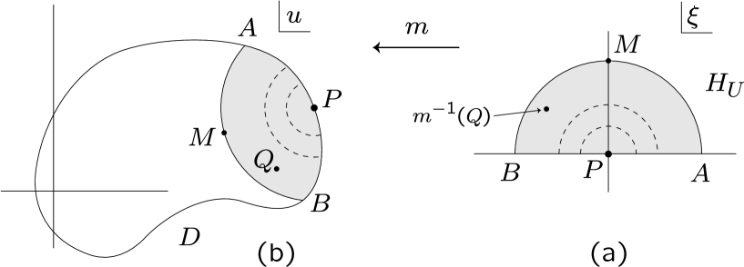
Figure 1: A punctured disk $D$ with a local coordinate around the puncture $P$. The coordinate is defined via a map from the half-disk $H_{U}$ to $D$. The arcs $AM$ and $MB$ in $D$ represent the left half and the right half of the open string respectively.

At an intuitive level $\langle\Sigma|$ can be given the following functional integral representation. Consider the path integral over the basic elementary fields of the two dimensional conformal field theory, $-$ collectively denoted as $\varphi$, $-$ on the disk $D$ minus the local coordinate patch, with some fixed boundary condition $\varphi=\varphi_{0}(\sigma)$ on the boundary $AMB$ of the local coordinate patch, and the open string boundary condition corresponding to the BCFT under study on the rest of the boundary of this region. The parameter $\sigma$ is the coordinate labeling the open string along $AMB$, defined through $\xi=e^{i\sigma}$. The result of this path integral will be a functional of the boundary value $\varphi_{0}(\sigma)$. We identify this as the wave-functional of the state $\langle\Sigma|$. (For describing the wave-functional of $|\Sigma\rangle$ we need to make a $\sigma\to(\pi-\sigma)$ transformation.) On the other hand the wave-functional of the state $|\phi\rangle$ can be obtained by performing the path integral over $\varphi$ on the unit half-disk in the $\xi$ coordinate system, with the boundary condition $\varphi=\varphi_{0}(\sigma)$ on the semicircle, open string boundary condition corresponding to the BCFT on real axis, and a vertex operator $\phi(0)$ inserted at the origin. We can now compute $\langle\Sigma|\phi\rangle$ for any state $|\phi\rangle$ in ${\cal H}$ by multiplying the two wave-functionals and integrating over the argument $\varphi_{0}(\sigma)$. The net result is a path integration over $\varphi$ on the full disk $D$, with the boundary condition corresponding to BCFT over the full boundary and a vertex operator $\phi$ inserted at the puncture $P$ using the $\xi$ coordinate system. This is precisely eq.(3.3).

3.1.2 The various pictures of the sliver

We are now ready to define the sliver surface state. Ref.[15] describes several canonical presentations of the sliver related by conformal tranformations. Here we shall review only three of them.

We begin by giving the description in which the disk $D$ is represented as the unit disk $D_{0}:|w|\leq 1$ in a $w$-plane. The puncture will be located at $w=1$. We define for any positive real number $n>0$

$$w_{n}=\check{f}_{n}(\xi)\equiv(h(\xi))^{2/n}=\Big{(}{1+i\xi\over 1-i\xi}\Big{)}^{2/n}\,,$$ (3.4)

which for later purposes we also write as

$$w_{n}=\exp\Bigl{(}\,i\,{4\over n}\,\tan^{-1}(\xi)\Bigr{)}\,.$$ (3.5)

The map $h(\xi)$ takes the canonical half disk into a unit half disk in the $h(\xi)$-plane, lying in the region $\Re(h(\xi))\geq 0$, $|h(\xi)|\leq 1$, with the puncture at $h(0)=1$ on the curved side of the half-disk. Moreover the string midpoint $M$ at $\xi=i$ is mapped to $h(i)=0$. The map $w_{n}=(h(\xi))^{2/n}$ makes the image of the canonical half-disk into a wedge with the angle at $w_{n}=0$ equal to $2\pi/n$. For any fixed $n$ we call the $\langle n|$ the resulting surface state. Thus we have

$$\langle n|\phi\rangle\equiv\langle\check{f}_{n}\circ\phi(0)\rangle_{D_{0}}\,\qquad\forall\phi.$$ (3.6)

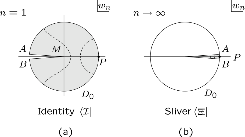
Figure 2: (a) The surface state corresponding to the identity string field $\langle{\cal I}|$. Here the image of $H_{U}$ covers the full disk, except for a cut in the negative real axis. (b) The surfaces state corresponding to the sliver $\langle\Xi|$. Here the image of $H_{U}$ covers an infinitesimally thin sliver around the positive real axis.

The state obtained when $n=1$ is the identity state (see Figure 2-a). For this state the local coordinate patch in the $w_{n}$ plane covers the full unit disk $D_{0}$ with a cut on the negative real axis. The left-half and the right-half of the string coincide along this cut. The state $n=2$ is the vacuum state. In this case the image of $H_{U}$ covers the right half of the full unit disk $D_{0}$ in the $w_{n}$ plane. In the $n\to\infty$ limit, the image of $H_{U}$ in the $w_{n}$ coordinate is a ‘thin sliver’ of the disk $D_{0}$ (Figure 2-b). It was seen in [21] and explained in detail in [15] that the limit $n\to\infty$ of $\langle n|$ gives rise to a well-defined state. The key is to use SL(2,R) invarainces to resolve the apparent singularity in the local coordinate as $n\to\infty$.

This surface state $\langle\Xi|$, called the sliver, has the property that the left-half and the right-half of the string are as far as they can be on the unit disk.

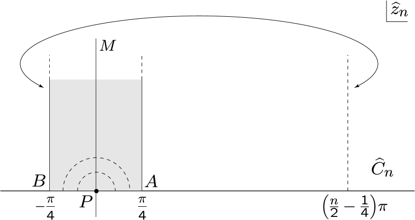
Figure 3: The finite $n$ approximation to the sliver presented in the $\widehat{z}_{n}$ coordinate.

In the second presentation of the wedge states $\langle n|$, we represent the disk $D$ in a new global coordinate system:

$$\widehat{w}_{n}=(w_{n})^{n/2}\,.$$ (3.7)

Under this map the unit disk $D_{0}$ in the $w_{n}$-coordinates is mapped to a cone in the $\widehat{w}_{n}$ coordinate, subtending an angle $n\pi$ at the origin $\widehat{w}_{n}=0$. We shall denote this cone by $\widehat{D}_{n}$. We see from (3.4) that

$$\widehat{w}_{n}=h(\xi)={1+i\xi\over 1-i\xi}\,.$$ (3.8)

Thus $\widehat{w}_{n}$ coordinate system has the special property that the local coordinate patch, i.e. the image of the half disk $H_{U}$ in $\widehat{D}_{n}$, is particularly simple. The image of $H_{U}$ appears as a vertical half-disk of unit radius, with the curved part of $H_{U}$ mapped to the imaginary axis and the diameter of $H_{U}$ mapped to the unit semi-circle to the right of the imaginary axis. Using eq.(3.8) we have

$$\langle n|\phi\rangle=\langle h\circ\phi(0)\rangle_{\widehat{D}_{n}}\,.$$ (3.9)

In the $n\to\infty$ limit $\widehat{D}_{n}$ can be viewed as an infinite helix.

Finally it is useful to introduce a new coordinate system

$$\widehat{z}_{n}={1\over 2i}\ln\widehat{w}_{n}\,.$$ (3.10)

The cone $\widehat{D}_{n}$ in the $\widehat{w}_{n}$ coordinate system maps to a semi-infinite cylinder $\widehat{C}_{n}$ in the $\widehat{z}_{n}$ coordinate system with $\widehat{z}_{n}$ spanning the range:

$$-{\frac{\pi}{4}}\leq\Re(\widehat{z}_{n})\leq(\frac{n}{2}-{1\over 4})\pi\,,\quad\Im(\widehat{z}_{n})\geq 0,\quad\widehat{z}_{n}\simeq\widehat{z}_{n}+n\,{\pi\over 2}\,.$$ (3.11)

The local coordinate patch is the region:

$$-{\pi/4}\leq\Re(\widehat{z}_{n})\leq{\pi/4},\quad\Im(\widehat{z}_{n})\geq 0\,.$$ (3.12)

This has been shown in Fig. 3. The relationship between $\widehat{z}_{n}$ and the local coordinate $\xi$ follows from eqs.(3.8) and (3.10):

$$\widehat{z}_{n}=\tan^{-1}\xi\equiv f(\xi)\,.$$ (3.13)

Thus we have

$$\langle n|\phi\rangle=\langle f\circ\phi(0)\rangle_{\widehat{C}_{n}}\quad\forall|\phi\rangle\in{\cal H}\,.$$ (3.14)

Note that using the periodicity along the $\Re(\widehat{z}_{n})$ direction we could take the range of $\Re(\widehat{z}_{n})$ to be $-n\pi/4\leq\Re(\widehat{z}_{n})\leq n\pi/4$. In this case as $n\to\infty$, $\widehat{C}_{n}$ approaches the full UHP and we get

$$\langle\Xi|\phi\rangle=\langle f\circ\phi(0)\rangle_{UHP}\,.$$ (3.15)

3.1.3 Star multiplication of wedge states

The star multiplication of two wedge states is easy to describe by representing them in the $\widehat{w}_{n}$ coordinate system. In this coordinate system the disk becomes a cone subtending an angle $\pi n$ at the origin. If we remove the local coordinate patch the left over region becomes a sector of angle $\pi(n-1)$. The star multiplication of two wedge states $|m\rangle*|n\rangle$ is readily performed by gluing the right half of the sector of angle $\pi(m-1)$ to the left half of the sector of angle $\pi(n-1)$. The result is of course a sector of angle $\pi(m+n-2)$. The local coordinate patch must then be restored to produce the full representation of the surface state. The result is a cone subtending an angle $\pi(m+n-1)$ at the origin, which corresponds to the wedge state $|m+n-1\rangle$ [21]:

$$|m\rangle*|n\rangle=|m+n-1\rangle\,.$$ (3.16)

In the limit $n,m\to\infty$ we find that the sliver squares to itself

$$\Xi*\Xi=\Xi\,.$$ (3.17)

We can now use the factorization property to conclude that the matter part of the sliver obeys $\Xi_{m}*^{m}\Xi_{m}=\Xi_{m}$, with suitable normalization of $\Xi_{m}$. (This could be infinite, but is universal in the sense that it does not depend on the specific choice of the matter BCFT, but only on the value $c=26$ of the central charge).

For later use it will be useful to work out the precise relationship between the different coordinate systems appearing in the description of the product state $|m+n-1\rangle$ and the states $|m\rangle$ and $|n\rangle$. Again this is simple in the $\widehat{w}$ coordinate system. For this let us take

$$\alpha=\pi(m-1),\qquad\beta=\pi(n-1),\qquad\alpha+\beta=\pi(m+n-2)\,,$$ (3.18)

and denote by ${\cal R}_{\alpha}$ and ${\cal R}_{\beta}$ the sectors of angles $\alpha$ and $\beta$ associated with the states $|m\rangle$ and $|n\rangle$ respectively. If we denote by $\widehat{w}_{m}$, $\widehat{w}_{n}$ and $\widehat{w}_{m+n-1}$ the $\widehat{w}$ coordinates associated with the wedge states $|m\rangle$, $|n\rangle$ and $|m+n-1\rangle$ respectively, we have

$$\widehat{w}_{m+n-1}=\cases{\widehat{w}_{m}\quad\,\,\,\,\,\,\hbox{in}\quad{\cal R}_{\alpha}\cr e^{i\alpha}\widehat{w}_{n}\quad\hbox{in}\quad{\cal R}_{\beta}\,\,.}$$ (3.19)

In the $\widehat{z}_{n}$ coordinate system introduced in eq.(3.10) the gluing relations (3.19) take a very simple form:

$$\widehat{z}_{m+n-1}=\cases{\widehat{z}_{m}\qquad\qquad\qquad\,\,\,\hbox{for}\quad{\pi\over 4}\leq\Re(\widehat{z}_{m})\leq(\frac{m}{2}-{1\over 4})\pi,\cr\cr\widehat{z}_{n}+{1\over 2}(m-1)\pi\quad\hbox{for}\quad{\pi\over 4}\leq\Re(\widehat{z}_{n})\leq(\frac{n}{2}-{1\over 4})\pi\,.}$$ (3.20)

3.2 The sliver as a squeezed state

Here we wish to review the construction of the matter part of the sliver in the oscillator representation and consider the basic algebraic properties that guarantee that the multiplication of two slivers gives a sliver. In fact we follow the discussion of Kostelecky and Potting [22] who gave the first algebraic construction of a state that would star multiply to itself in the matter sector. This discussion was simplified in [13] where due attention was also paid to normalization factors that guarantee that the states satisfy precisely the projector equation (2.8). We also identify some infinite dimensional matrices introduced in [14] with the properties of projection operators. These matrices will be useful in the construction of multiple D-brane solutions in section 5.

In order to star multiply two states $|A\rangle$ and $|B\rangle$ we must calculate

$$(|A\rangle*|B\rangle)_{3}={}_{1}\langle A|{}_{2}\langle B|V_{3}\rangle_{123}\,,$$ (3.21)

where $|~{}\rangle_{r}$ denotes a state in the $r$-th string Hilbert space, and $|~{}\rangle_{123}$ denotes a state in the product of the Hilbert space of three strings. The key ingredient here is the three-string vertex $|V_{3}\rangle_{123}$. While the vertex has nontrivial momentum dependence, if the states $A$ and $B$ are at zero momentum, the star product gives a zero momentum state that can be calculated using

$$|V_{3}\rangle_{123}=\exp\Bigl{(}-{1\over 2}\sum_{{r,s}}a^{(r)\dagger}\cdot V^{rs}\cdot a^{(s)\dagger}\Bigr{)}|0\rangle_{123}\,,$$ (3.22)

and the rule $\langle 0|0\rangle=1$. Here the $V^{rs}$, with $r,s=1,2,3$, are infinite matrices $V^{rs}_{mn}$ ($m,n=1,\cdots\infty$) satisfying the cyclicity condition $V^{rs}=V^{r+1,s+1}$ and the symmetry condition $(V^{rs})^{T}=V^{sr}$. These properties imply that out of the nine matrices, three: $V^{11},V^{12}$ and $V^{21}$, can be used to obtain all others. $a^{(r)\mu\dagger}_{m}$ ($0\leq\mu\leq 25$) denote oscillators in the $r$-th string Hilbert space. For simplicity, the Lorentz and the oscillator indices, and the Minkowski matrix $\eta_{\mu\nu}$ used to contract the Lorentz indices, have all been suppressed in eq.(3.22). We shall follow this convention throughout the paper.

One now introduces

$$M^{rs}\equiv CV^{rs}\,,\quad\hbox{with}\quad C_{mn}=(-1)^{m}\delta_{mn},\quad m,n\geq 1\,.$$ (3.23)

These matrices can be shown to satisfy the following properties:

$$CV^{rs}=V^{sr}C\,,\quad(V^{rs})^{T}=V^{sr}\,,$$

$$(M^{rs})^{T}=M^{rs}\,,\quad CM^{rs}C=M^{sr}\,,\quad[M^{rs},M^{r^{\prime}s^{\prime}}]=0\,.$$ (3.24)

In particular note that all the $M$ matrices commute with each other. Defining $X\equiv M^{11}$, the three relevant matrices are $X,M^{12}$ and $M^{21}$. Explicit formulae exist that allow their explicit computation [32, 33]. In particular they obey the relations:

$$M^{12}+M^{21}=1-X\,,\quad M^{12}M^{21}=X^{2}-X\,.$$ (3.25)

The state in the matter Hilbert space that multiplies to itself takes the form [22, 13]

$$|\Psi\rangle={\cal N}^{26}\exp\Bigl{(}-{1\over 2}\,a^{\dagger}\cdot S\cdot a^{\dagger}\Bigr{)}|0\rangle\,,\quad{\cal N}=\{\det(1-X)\det(1+T)\}^{1/2}\,,\quad S=CT$$ (3.26)

where the matrix $T$ satisfies $CTC=T$ and the equation

$$XT^{2}-(1+X)T+X=0\,,$$ (3.27)

which gives

$$T=(2X)^{-1}(1+X-\sqrt{(1+3X)(1-X)}).$$ (3.28)

In taking the square root we pick that branch which, for small $X$, goes as $(1+X)$.

In [13] we identified this state as the sliver by computing numerically the matrix $S$ using the equation above and comparing the state obtained this way with the matter part of the sliver $|\Xi\rangle$, which can be evaluated directly using the techniques of ref.[36]. We found close agreement between the numerical values of $S_{mn}$ and exact answers for $\widehat{S}_{mn}$. This gave convincing evidence that $|\Psi\rangle=|\Xi\rangle$.

The algebraic structure allows one to construct a pair of projectors that have the interpretation of projectors into the left and right halves of a string. We define the matrices

$$\displaystyle\rho_{1} ={1\over(1+T)(1-X)}\Bigl{[}M^{12}(1-TX)+T(M^{21})^{2}\Bigr{]}\,,$$ (3.29)

$$\rho_{2} ={1\over(1+T)(1-X)}\Bigl{[}M^{21}(1-TX)+T(M^{12})^{2}\Bigr{]}\,.$$

One can verify, using various identities satisfied by $X$, $M^{12}$ and $M^{21}$, that they satisfy the following properties:

$$\rho_{1}+\rho_{2}=1,\quad\rho_{1}^{T}=\rho_{1}\,,\quad\rho_{2}^{T}=\rho_{2}\,,\quad C\rho_{1}C=\rho_{2}\,,$$ (3.30)

and more importantly

$$\rho_{1}\rho_{1}=\rho_{1}\,,\quad\rho_{2}\rho_{2}=\rho_{2}\,.$$ (3.31)

We see that $\rho_{1}$ and $\rho_{2}$ are projection operators into orthogonal complementary subspaces exchanged by $C$.

With the help of these projectors one can compute some useful star products. For example, introducing coherent like states of the form

$$|\Xi_{\beta}\rangle=\exp\Bigl{(}\sum_{n=1}^{\infty}(-)^{n+1}\beta_{\mu n}a_{n}^{\mu\dagger}\Bigr{)}|\Xi\rangle=\exp(-a^{\dagger}\cdot C\beta)|\Xi\rangle\,,$$ (3.32)

one can show [14] that

$$|\Xi_{\beta_{1}}\rangle*|\Xi_{\beta_{2}}\rangle=\exp\Bigl{(}-{\cal C}(\beta_{1},\beta_{2})\Bigr{)}|\Xi_{\rho_{1}\beta_{1}+\rho_{2}\beta_{2}}\rangle\,,$$ (3.33)

where

$$\displaystyle{\cal C}(\beta_{1},\beta_{2})={1\over 2}\,(\beta_{1},\beta_{2}){1\over(1+T)(1-X)}\pmatrix{V^{11}(1-T)&V^{12}\cr V^{21}&V^{11}(1-T)}\pmatrix{\beta_{1}\cr\beta_{2}}\,.$$ (3.34)

(3.33) is a useful relation that allows one to compute $*$-products of slivers acted by oscillators by simple differentiation. For example,

$$\displaystyle(a^{\mu\dagger}_{m}|\Xi\rangle)*(a^{\nu\dagger}_{n}|\Xi\rangle)=(-1)^{(m+1)+(n+1)}\Bigl{(}{\partial\over\partial\beta_{1\mu m}}{\partial\over\partial\beta_{2\nu n}}\big{(}|\Xi_{\beta_{1}}\rangle*|\Xi_{\beta_{2}}\rangle\big{)}\Bigr{)}_{\beta_{1}=\beta_{2}=0}\,.$$ (3.35)

It follows from (3.33) that $P_{\beta}\equiv\exp\Bigl{(}{\cal C}(\beta,\beta)\Bigr{)}|\Xi_{\beta}\rangle$ satisfies $P_{\beta}*P_{\beta}=P_{\beta}\,$. One can also check that $\langle P_{\beta}|P_{\beta}\rangle=\langle\Xi|\Xi\rangle\,$.

4 Boundary CFT construction of D-brane solutions

In this section we shall review the basic construction of [15]. We shall describe deformations of the sliver to generate new solutions of the equations of motion representing D-branes described by general BCFT’s. The general idea is simple. We denote by BCFT₀ the reference BCFT in whose Hilbert space the string field takes value. The D-brane associated with BCFT₀ is represented by a solution of the string field equation (2.6) whose matter part is the sliver of BCFT₀, $-$ the surface state described in section 3.1, with the specific boundary condition corresponding to BCFT₀ on the boundary of the surface. To get a solution representing the single D-brane of some other boundary conformal field theory BCFT^′ we must represent the sliver of BCFT^′ on the state space of BCFT₀, as we now explain. The construction assumes that BCFT₀ and BCFT^′ have the same bulk conformal field theory, but of course, differ in their boundary interactions.

Usually the sliver $\Xi^{\prime}$ of BCFT^′ will be described in the same manner as discussed in the last section, with all the correlation functions now being calculated in BCFT^′. This, however, would express $\Xi^{\prime}$ as a state in the state space ${\cal H}^{\prime}$ of BCFT^′, since in eq. (3.15), for example, $\phi$ will now represent a vertex operator of BCFT^′. In order to express $\Xi^{\prime}$ in the state space of BCFT₀, we adopt the following procedure. As discussed in section 3.1.1, at an intuitive level, the wave-functional for $\langle\Xi^{\prime}|$ is a functional of $\varphi_{0}(\sigma)$ with $\sigma$ labeling the coordinate along the string, obtained by functional integration over the two dimensional fields $\varphi$ on the full disk (UHP labeled by $z^{\prime}=\tan^{-1}\xi$ in this case) minus the local coordinate patch ($|\Re(z^{\prime})|\leq\pi/4$), with boundary condition $\varphi=\varphi_{0}(\sigma)$ on the boundary $\xi=e^{i\sigma}$ ($\Re(z^{\prime})=\pm\pi/4$), and the boundary condition appropriate to BCFT^′ on the rest of the boundary of this region ($z^{\prime}$ real, $|\Re(z^{\prime})|\geq\pi/4$). On the other hand given a state $|\phi\rangle$ in the Hilbert space ${\cal H}$ of BCFT₀, we represent the wave-functional of $|\phi\rangle$ as a functional of $\varphi_{0}(\sigma)$, obtained by performing path integral over $\varphi$ in the inside of the local coordinate patch with boundary condition appropriate for BCFT₀ on the real axis, the vertex operator $\phi$ of BCFT₀ inserted at the origin in the local coordinate system $\xi$, and the boundary condition $\varphi=\varphi_{0}(\sigma)$ on the semi-circle $\xi=e^{i\sigma}$. Finally in order to calculate $\langle\Xi^{\prime}|\phi\rangle$ we take the product of the wave-functional of $\langle\Xi^{\prime}|$ and the wave-functional of $|\phi\rangle$ and integrate over $\varphi_{0}(\sigma)$. The result will be a functional integral over the fields $\varphi$ on the full UHP, with boundary condition appropriate to BCFT^′ in the range $|\Re(z^{\prime})|\geq\pi/4$, boundary condition corresponding to BCFT₀ for $|\Re(z^{\prime})|\leq\pi/4$ and the vertex operator $\phi$ inserted at the origin in the local coordinate system. This can be expressed as

$$\langle\Xi^{\prime}|\phi\rangle=\langle f\circ\phi(0)\rangle^{\prime\prime}\,,$$ (4.1)

where $\langle~{}\rangle^{\prime\prime}$ denotes correlation function in a theory where we have BCFT^′ boundary condition for $|\Re(z^{\prime})|\geq\pi/4$ and BCFT₀ boundary condition for $|\Re(z^{\prime})|\leq\pi/4$. $\phi$ is a vertex operator in BCFT₀ and $f(\xi)=\tan^{-1}\xi$ as usual.

In what follows, we shall show that after appropriate ultraviolet regularization, $\Xi^{\prime}$ defined this way squares to itself under $*$-multiplication, and also has the right tension for describing a D-brane associated to BCFT^′. We will only review this general case in the next subsections. We refer to [15] for the discussion of the case where BCFT^′ is replaced by a general two dimensional field theory obtained from BCFT₀ by some boundary perturbation.

4.1 Solution describing an arbitrary D-brane

We shall now describe the construction of the solution of the SFT equations of motion describing a D-brane corresponding to an arbitrary boundary conformal field theory BCFT^′ with the same bulk CFT as BCFT₀. We start with the definition of $\Xi^{\prime}$ given in eq.(4.1). The effect of the change of the boundary condition beyond $|x^{\prime}|\geq\pi/4$ can be represented by inserting boundary condition changing vertex operator $\sigma^{\pm}$ (discussed e.g. in [25, 26]) at $x^{\prime}=\pm\pi/4$. In other words we can express (4.1) as

$$\langle\Xi^{\prime}|\phi\rangle=\Bigl{\langle}f\circ\phi(0)\,\sigma^{+}({\pi\over 4})\sigma^{-}(-{\pi\over 4})\Bigr{\rangle}\,.$$ (4.2)

If we denote by D and D^′ the D-branes associated with BCFT₀ and BCFT^′ respectively, then $\sigma^{+}$ denotes the vertex operator for the ground state of an open string whose left end (viewed from inside the UHP) is on the D^′-brane and right end is on the D-brane, whereas $\sigma^{-}$ denotes the vertex operator for the ground state of open string whose left end is on the D-brane and right end is on the D^′-brane. In anticipation of short-distance divergences, we shall actually put $\sigma^{-}$ and $\sigma^{+}$ at $(-{\pi\over 4}-\epsilon)$ and $({\pi\over 4}+\epsilon)$ respectively, where $\epsilon$ is a small positive number. We shall also use the description of the sliver as limit of finite $n$ wedge states in the $\widehat{z}_{n}$ coordinate introduced in eq.(3.10). Thus we have

$$\langle\Xi^{\prime}|\phi\rangle=\lim_{n\to\infty}\Bigl{\langle}f\circ\phi(0)\,\sigma^{+}\Bigl{(}{\pi\over 4}+\epsilon\Bigr{)}\sigma^{-}\Bigl{(}{n\over 2}\pi-{\pi\over 4}-\epsilon\Bigr{)}\Bigr{\rangle}_{\widehat{C}_{n}}\,.$$ (4.3)

We now calculate $\Xi^{\prime}*\Xi^{\prime}$. From the gluing relations (3.20) we get,

$$\displaystyle\langle\Xi^{\prime}*\Xi^{\prime}|\phi\rangle = \lim_{m,n\to\infty}\Biggl{\langle}f\circ\phi(0)\,\,\sigma^{+}\Bigl{(}{\pi\over 4}+\epsilon\Bigr{)}\,\sigma^{-}\Bigl{(}({m\over 2}-{1\over 4})\pi-\epsilon\Bigr{)}$$ (4.4)

$$\sigma^{+}\Bigl{(}({m\over 2}-{1\over 4})\pi+\epsilon\Bigr{)}\sigma^{-}\Bigl{(}{1\over 2}(m+n-1)\pi-{\pi\over 4}-\epsilon\Bigr{)}\Biggr{\rangle}_{\widehat{C}_{m+n-1}}\,.$$

Thus the $\sigma^{\pm}$ at ${1\over 2}(m-{1\over 2})\pi\pm\epsilon$ come close as $\epsilon\to 0$ and give rise to a divergent factor $(2\epsilon)^{-2h}$ where $h$ is the conformal weight of $\sigma^{\pm}$. Hence we have $\Xi^{\prime}*\Xi^{\prime}=(2\epsilon)^{-2h}\Xi^{\prime}$. This requires us to redefine $\Xi^{\prime}$ by absorbing a factor of $(2\epsilon)^{2h}$, so that it squares to itself under $*$-multiplication

$$\Xi^{\prime}_{R}\equiv(2\epsilon)^{2h}\,\,\Xi^{\prime}\quad\to\quad\Xi^{\prime}_{R}*\Xi^{\prime}_{R}=\Xi^{\prime}_{R}\,.$$ (4.5)

We note, however, that even for finite $\epsilon$, the state $\Xi^{\prime}_{R}$ still squares to itself. Indeed, the product $\sigma^{-}({1\over 2}(m-{1\over 2})\pi-\epsilon)\sigma^{+}({1\over 2}(m-{1\over 2})\pi+\epsilon)$ can be expanded in an operator product expansion, and since these operators are moved to $\infty$ in the $m,n\to\infty$ limit, only the identity operator in this operator product expansion would contribute. The coefficient of the identity operator is given by $(2\epsilon)^{-2h}$ even for finite $\epsilon$.

Since BCFT₀ and BCFT^′ differ only in the matter sector, it is clear that $|\Xi^{\prime}_{R}\rangle$ has the factorized form

$$|\Xi^{\prime}_{R}\rangle=|\Xi_{g}\rangle\otimes|\Xi^{\prime}_{R,m}\rangle\,,$$ (4.6)

where $\Xi_{g}$ is a universal ghost factor. Normalizing $\Xi_{g}$ (which is independent of the choice of BCFT^′) such that $\Xi_{g}*^{g}\Xi_{g}=\Xi_{g}$, we can ensure that

$$\Xi^{\prime}_{R,m}*^{m}\Xi^{\prime}_{R,m}=\Xi^{\prime}_{R,m}\,.$$ (4.7)

Thus we can now construct a new D-brane solution by taking the product $|\Psi_{g}\rangle\otimes|\Xi^{\prime}_{R,m}\rangle$, where $|\Psi_{g}\rangle$ is the same universal ghost state that appears in the construction of the D-brane solution corresponding to BCFT₀.

We shall now calculate the tension associated with this new D-brane solution. For this we need to compute $\langle\Xi_{R,m}^{\prime}|\Xi_{R,m}^{\prime}\rangle_{m}$, where the subscript $m$ denotes matter. We have,

$$\langle\Xi_{R,m}^{\prime}|\Xi_{R,m}^{\prime}\rangle_{m}=(2\epsilon)^{4h}\,\,\langle\Xi_{m}^{\prime}|\Xi_{m}^{\prime}\rangle_{m}\,.$$ (4.8)

Calculation of $\langle\Xi_{m}^{\prime}|\Xi_{m}^{\prime}\rangle_{m}$ is again simple in the $\widehat{z}_{n}$ coordinate system. We first compute the $*$-product of the two states, and then in the final glued surface with coordinate $\widehat{z}_{m+n-1}$ we remove the local coordinate patch $-\pi/4\leq\Re(\widehat{z}_{m+n-1})\leq\pi/4$ and identify the lines $\Re(\widehat{z}_{m+n-1})=\pm\pi/4$. This produces the semi-infinite cylinder $\widetilde{C}_{m+n-2}$ defined by ${\pi\over 4}\leq\Re(z_{m+n-2})\leq{\pi\over 4}+(m+n-2){\pi\over 2}$ and $\Im(z_{m+n-2})\geq 0$. We therefore find

$$\displaystyle\langle\Xi_{m}^{\prime}|\Xi_{m}^{\prime}\rangle_{m} = \lim_{m,n\to\infty}\Biggl{\langle}\sigma^{+}\Bigl{(}{\pi\over 4}+\epsilon\Bigr{)}\,\,\sigma^{-}\Bigl{(}({m\over 2}-{1\over 4})\pi-\epsilon\Bigr{)}$$ (4.9)

$$\sigma^{+}\Bigl{(}{m\over 2}-{1\over 4})\pi+\epsilon\Bigr{)}\sigma^{-}\Bigl{(}{1\over 2}(m+n-1)\pi-{\pi\over 4}-\epsilon\Bigr{)}\Bigg{\rangle}_{\widetilde{C}_{m+n-2}}\,,$$

where the correlation function is now being computed in the matter BCFT. We get a factor of $(2\epsilon)^{-2h}$ coming from $\sigma^{\pm}$ inserted at $({m\over 2}-{1\over 4})\pi\pm\epsilon$ as before, but there is another factor of $(2\epsilon)^{-2h}$ coming from the other $\sigma^{\pm}$ insertions that happen at points separated by a (minimal) distance $2\epsilon$ on the cylinder $\widetilde{C}_{m+n-2}$. These exactly cancel the explicit factor of $(2\epsilon)^{4h}$ in (4.8). Since from the definition of $\sigma^{\pm}$ it is clear that in the $\epsilon\to 0$ limit we have BCFT^′ boundary condition on the full real $z_{m+n-2}$ axis, we find that $\langle\Xi^{\prime}_{R,m}|\Xi_{R,m}^{\prime}\rangle_{m}$ is given by the partition function of the deformed boundary CFT on the $\widetilde{C}_{m+n-2}$ cylinder

$$\langle\Xi_{R,m}^{\prime}|\Xi_{R,m}^{\prime}\rangle_{m}=Z_{\widetilde{C}_{m+n-2}}(\hbox{BCFT}^{\prime})\sim Z_{D_{0}}(\hbox{BCFT}^{\prime})\,,$$ (4.10)

where in the last step we relate this partition function to the one on the standard unit disk. This is possible because of conformal invariance. Any constant multiplicative factor that might appear due to conformal anomaly depends only on the bulk central charge and is independent of the choice of BCFT^′. This can at most give rise to a universal multiplicative factor. Since the partition function of BCFT^′ on the unit disk is proportional to the tension of the corresponding D-brane [23] $-$ a fact which has played a crucial role in the analysis of tachyon condensation in boundary string field theory[9, 10], $-$ we see that the tension $\langle\Xi_{R,m}^{\prime}|\Xi_{R,m}^{\prime}\rangle_{m}$ computed from vacuum string field theory agrees with the known tension of the BCFT^′ D-brane, up to an overall constant factor independent of BCFT^′.

Arguments similar to the one given for $\Xi^{\prime}*\Xi^{\prime}$ show that the result (4.10) holds even when $\epsilon$ is finite. In this case we have two pairs of $\sigma^{\pm}$ on the boundary, with the first pair being infinite distance away from the second pair. Thus we can expand each pair using operator product expansion and only the identity operator contributes, giving us back the partition function of BCFT^′ on the disk. From this we see that we have a one parameter family of solutions, labeled by $\epsilon$, describing the same D-brane. We expect these solutions to be related by gauge transformations.

4.2 Multiple D-branes and coincident D-branes

We first consider the construction of a configuration containing various D-branes associated to different BCFT^′s. To this end, we note that the star product $\Xi^{\prime}*\Xi$ of the BCFT^′ solution and the BCFT₀ solution vanishes. Indeed, using the same methods as in the previous subsection, the computation of $\langle\Xi^{\prime}*\Xi|\phi\rangle$ leads to the cylinder $\widehat{C}_{m+n-1}$ with a $\sigma^{+}$ insertion at ${\pi\over 4}+\epsilon$, a $\sigma^{-}$ insertion at $({m\over 2}-{1\over 4})-\epsilon$, and $f\circ\phi(0)$ insertion at $f(0)=0$. In the $m,n\to\infty$ limit, $\sigma^{-}$ moves off to infinity and as a result the correlation function vanishes since $\sigma^{-}$ has dimension larger than zero as long as BCFT₀ and BCFT^′ are different. Similar arguments show that $\Xi*\Xi^{\prime}$ and $\langle\Xi_{m}|\Xi^{\prime}_{m}\rangle_{m}$ also vanish. Thus the matter part of $\Xi+\Xi^{\prime}_{R}$ is a new solution describing the superposition of the D-branes corresponding to BCFT₀ and BCFT^′. Since no special assumptions were made about BCFT₀ or BCFT^′, it follows that $\Xi^{\prime}*\Xi^{\prime\prime}=\Xi^{\prime\prime}*\Xi^{\prime}=0$ and $\langle\Xi^{\prime}_{m}|\Xi^{\prime\prime}_{m}\rangle_{m}=0$ for any two different BCFT^′ and BCFT^′′, and hence we can superpose any number of slivers to form a solution. This in particular also includes theories which differ from each other by a small marginal deformation. Special cases of this phenomenon, in the case of D-branes in flat space-time, have been discussed in ref.[17].

This procedure, however, is not suitable for superposing D-branes associated with the same BCFT, i.e. for parallel coincident D-branes. For example, if we take BCFT^′ to differ from BCFT₀ by an exactly marginal deformation with deformation parameter $\lambda$, then in the $\lambda\to 0$ limit the operators $\sigma^{\pm}$ both approach the identity operator (having vanishing conformal weight), and although the argument for the vanishing of $\Xi*\Xi^{\prime}$ holds for any non-zero $\lambda$, it breaks down at $\lambda=0$.

In order to construct a superposition of identical D-branes, one can proceed in a different way. First consider getting coincident BCFT₀ branes. To this end we introduce a modified BCFT₀ sliver

$$\langle\Xi_{\chi}|\phi\rangle=\lim_{n\to\infty}\Bigl{\langle}f\circ\phi(0)\,\chi^{+}\Bigl{(}{\pi\over 4}+\epsilon\Bigr{)}\chi^{-}\Bigl{(}{n\over 2}\pi-{\pi\over 4}-\epsilon\Bigr{)}\Bigr{\rangle}_{\widehat{C}_{n}}\,.$$ (4.11)

Here $\chi^{\pm}$ are a conjugate pair of operators of BCFT₀, having a common dimension $h$ greater than zero, and representing some excited states of the open string with both ends having BCFT₀ boundary condition. Thus, throughout the real line we have BCFT₀ boundary conditions. We require that the coefficient of the identity in the OPE $\chi^{-}(x)\chi^{+}(y)$ is given by $|x-y|^{-2h_{i}}$, and that this OPE does not contain any other operator of dimension $\leq 0$.

The clear parallel between eqn. (4.11) and eqn. (4.3), describing the BCFT^′ D-brane, implies that an analysis identical to the one carried out in the previous section will show that:

1. This new state $\Xi_{\chi}$ (after suitable renormalization as in eq.(4.5)) squares to itself under $*$-multiplication.

2. The BPZ norm of the matter part of $\Xi_{\chi}$ is proportional to the partition function of BCFT₀ on the unit disk.

3. $\Xi_{\chi}$ has vanishing $*$-product with $\Xi$.

Thus the matter part of this state gives another representation of the D-brane associated with BCFT₀, and we can construct a pair of D-branes associated with BCFT₀ by superposing the matter parts of $\Xi$ and $\Xi_{\chi}$.

This construction can be easily generalized to describe multiple BCFT₀ D-branes. We construct different representations of the same D-brane by using different vertex operators $\chi^{(i)\pm}$ in BCFT₀ satisfying the ‘orthonormality condition’ that the coefficient of the identity operator in the OPE of $\chi^{(i)-}(x)\chi^{(j)+}(y)$ is given by $\delta_{ij}|x-y|^{-2h_{i}}$, and that this OPE does not contain any other operator of dimension $\leq 0$. The correponding solutions $\Xi_{\chi^{(i)}}$ all have vanishing $*$-product with each other, and hence can be superposed to represent multiple D-branes associated with BCFT₀.

For constructing a general configuration of multiple D-branes some of which may be identical and some are different, we choose a set of conjugate pair of vertex operators $\chi^{(i)\pm}$, representing open strings with one end satisfying boundary condition corresponding to BCFT₀ and the other end satisfying the boundary condition corresponding to some boundary conformal field theory BCFT_i, satisfying the ‘orthonormality condition’ that the coefficient of the identity operator in the OPE of $\chi^{(i)-}(x)\chi^{(j)+}(y)$ is given by $\delta_{ij}|x-y|^{-2h_{i}}$, and that this OPE does not contain any other operator of dimension $\leq 0$. The correponding solutions $\Xi_{\chi^{(i)}}$ all have vanishing $*$-product with each other, and hence can be superposed to represent multiple D-branes, with the $i$th D-brane being associated with BCFT_i. Since there is no restriction that BCFT_i should be different from BCFT₀, or from BCFT_j for $j\neq i$, we can use this procedure to describe superposition of an arbitrary set of D-branes.

This procedure of adding vertex operators near $\pm\pi/4$ to create new solutions representing the same D-brane is the BCFT version of the use of excited states of half-strings [14, 17] for the same purpose. This is reviewed in section 5.

4.3 Solutions from boundary field theories

We can consider a class of solutions associated with the sliver for boundary field theories which are not necessarily conformal. For this, suppose $V$ is a local vertex operator in the matter sector of BCFT₀ and define a new state $\langle\Xi^{V,\lambda}|$ through the relation:

$$\langle\Xi^{V,\lambda}|\phi\rangle=\lim_{n\to\infty}\Big{\langle}\exp\Big{(}-\lambda\int_{{\pi\over 4}}^{({n\over 2}-{1\over 4})\pi}V(x_{n})dx_{n}\Big{)}f\circ\phi(0)\Big{\rangle}_{\widehat{C}_{n}}\quad\forall|\phi\rangle\in{\cal H}\,,$$ (4.12)

where $x_{n}=\Re(\widehat{z}_{n})$, $\lambda$ is a constant, and the integration is done over the real $\widehat{z}_{n}$ axis excluding the part that is inside the local coordinate patch. This expression should be treated as a correlation function in a theory where on part of the boundary we have the usual boundary action corresponding to BCFT₀, and on part of the boundary we have a modified boundary action obtained by adding the integral of $V$ to the original action (in defining this we need to use suitable regularization and renormalization prescriptions; see ref.[15] for more discussion of this). Alternatively, we have a correlation function with BCFT₀ boundary condition in the range $-{\pi\over 4}\leq x\leq{\pi\over 4}$ and a modified boundary condition outside this range.

One can show that $|\Xi^{V,\lambda}\rangle$ satisfies the projection equation $\Xi^{V,\lambda}*\Xi^{V,\lambda}=\Xi^{V,\lambda}$, by using the $\widehat{z}_{n}$ coordinate system to take the star product [15]. This may be surprising given that $V$ is not constrained, but is a consequence of the trivial way the star product acts in the $\widehat{z}_{n}$ coordinates . Since the operator $V$ is in the matter sector, $\Xi^{V,\lambda}$ has the usual ghost/matter factorized form, and the matter part satisfies $\Xi^{V,\lambda}_{m}*^{m}\Xi^{V,\lambda}_{m}=\Xi^{V,\lambda}_{m}\,$. Thus we can now construct new D-brane solutions by taking the product $|\Psi_{g}\rangle\otimes|\Xi^{V,\lambda}_{m}\rangle$, where $|\Psi_{g}\rangle$ is the universal ghost state that appears in the D25-brane solution.

The tension associated with such solution is proportional to $\langle\Xi_{m}^{V,\lambda}|\Xi_{m}^{V,\lambda}\rangle_{m}$. This computation is again simple in the $\widehat{z}_{n}$ coordinates and the relevant geometry was discussed above (4.9). One finds

$$\langle\Xi_{m}^{V,\lambda}|\Xi_{m}^{V,\lambda}\rangle_{m}=\lim_{m,n\to\infty}\Bigl{\langle}\exp\Big{(}-\lambda\int_{{\pi\over 4}}^{{m+n-1\over 2}\pi-{\pi\over 4}}V(x_{m+n-2})dx_{m+n-2}\Big{)}\Bigr{\rangle}_{\widetilde{C}_{m+n-2}}\,,\\$$

where $x_{m+n-2}=\Re(z_{m+n-2})$. We now define a rescaled coordinate $u$ as $u=4(z_{m+n-2}-{\pi\over 4})/(m+n-2)$ so that $\Re(u)$ ranges from 0 to $2\pi$. Thus in the $u$ coordinate we have a semiinfinite cylinder $C$ of circumference $2\pi$. Writing $u=i\rho+\theta$, and taking into account the conformal transformation of the vertex operator $V$ under this scale transformation, we get:

$$\langle\Xi_{m}^{V,\lambda}|\Xi_{m}^{V,\lambda}\rangle=\lim_{m,n\to\infty}\Bigl{\langle}\exp\Big{(}-\lambda_{R}\int_{\theta=0}^{2\pi}d\theta V_{R}(\theta)\Big{)}\Bigr{\rangle}_{C}\,,$$ (4.13)

where $\lambda_{R}\int V_{R}$ denotes the operator to which the perturbation $\lambda\int V$ flows under the rescaling by $(m+n-2)/4$. This semiinfinite cylinder in the $u$ coordinate is nothing but a unit disk $D_{U}$ with $\theta$ labeling the angular parameter along the boundary of the disk, and $e^{-\rho}$ labeling the radial coordinate. Thus (4.13) is the partition function on a unit disk, with the perturbation $\lambda_{R}\int V_{R}(\theta)d\theta$ added at the boundary! If $V$ is a relevant deformation then $h<1$ and in the limit $m,n\to\infty$, $\lambda_{R}\int d\theta V_{R}(\theta)$ approaches its infrared fixed point $\lambda_{IR}\int d\theta V_{IR}(\theta)$. Thus, $\langle\Xi_{m}^{V,\lambda}|\Xi_{m}^{V,\lambda}\rangle_{m}$ represents the partition function on the unit disk of the BCFT to which the theory flows in the infrared! This is indeed the tension of the D-brane associated to this BCFT. Thus $|\Psi_{g}\rangle\otimes|\Xi_{m}^{V,\lambda}\rangle$ is the D-brane solution for the BCFT obtained as the infrared fixed point of the boundary perturbation $\int V(\theta)d\theta$.

5 Half strings, projectors and multiple D25-branes in the algebraic approach

In this section we review the basic ideas of [14] $-$ see also [17]. First we consider the functional representation of the $*$-product and argue that it is natural to think of string fields as operators acting in the space of half string functionals. This intuition provides the clue for a rigorous algebraic construction of multiple D-brane solutions. Throughout this section we shall deal with matter sector states only, and compute $*$-products and BPZ inner products in the matter sector, but will drop the subscripts and superscripts $m$ from the labels of the states, $*$-products and inner products.

5.1 Half-string functionals and projectors

We shall begin by examining the representation of string fields as functionals of half strings. This viewpoint is possible at least for the case of zero momentum string fields. It leads to the realization that the sliver functional factors into functionals of the left and right halves of the string, allowing its interpretation as a rank-one projector in the space of half-string functionals. We construct higher rank projectors – these are solution of the equations of motion representing multiple D25-branes.

5.1.1 Zero momentum string field as a matrix

The string field equation in the matter sector is given by

$$\Psi*\Psi=\Psi\,.$$ (5.1)

Thus if we can regard the string field as an operator acting on some vector space where $*$ has the interpretation of product of operators, then $\Psi$ is a projection operator in this vector space. Furthermore, in analogy with the results in non-commutative solitons [37] we expect that in order to describe a single D-brane, $\Psi$ should be a projection operator into a single state in this vector space.

A possible operator interpretation of the string field was suggested in Witten’s original paper [2], and was further developed in refs.[28, 29]. In this picture the string field is viewed as a matrix where the role of the row index and the column index are taken by the left-half and the right-half of the string respectively. In order to make this more concrete, let us consider the standard mode expansion of the open string coordinate [32]:

$$X^{\mu}(\sigma)=x^{\mu}_{0}+\sqrt{2}\sum_{n=1}^{\infty}x^{\mu}_{n}\cos(n\sigma)\,,\quad\hbox{for}\quad 0\leq\sigma\leq\pi\,.$$ (5.2)

Now let us introduce coordinates $X^{L\mu}$ and $X^{R\mu}$ for the left and the right half of the string as follows:

$$\displaystyle X^{L\mu}(\sigma) = X^{\mu}(\sigma/2)-\,\,X^{\mu}(\pi/2)\,\,,\,\,\qquad\hbox{for}\quad 0\leq\sigma\leq\pi\,.$$

$$X^{R\mu}(\sigma) = X^{\mu}(\pi-\sigma/2)-X^{\mu}(\pi/2),\qquad\hskip-9.0pt\hbox{for}\quad 0\leq\sigma\leq\pi\,.$$ (5.3)

$X^{L\mu}(\sigma)$ and $X^{R\mu}(\sigma)$ satisfy the usual Neumann boundary condition at $\sigma=0$ and a Dirichlet boundary condition at $\sigma=\pi$. Thus they have expansions of the form:

$$\displaystyle X^{L\mu}(\sigma) = \sqrt{2}\sum_{n=1}^{\infty}x^{L\mu}_{n}\cos((n-{1\over 2})\sigma),$$ (5.4)

$$X^{R\mu}(\sigma) = \sqrt{2}\sum_{n=1}^{\infty}x^{R\mu}_{n}\cos((n-{1\over 2})\sigma)\,.$$

Comparing (5.2) and (5.4) we get an expression for the full open string modes in terms of the modes of the left-half and the modes of the right-half:

$$x^{\mu}_{n}=A_{nm}^{+}\,x^{L\mu}_{m}+A^{-}_{nm}\,x^{R\mu}_{m},\qquad m,n\geq 1\,,$$ (5.5)

where the matrices $A^{\pm}$ are

$$A_{nm}^{\pm}=\pm{1\over 2}\delta_{n,2m-1}+{1\over 2\pi}\epsilon(n,m)\Big{(}{1\over 2m+n-1}+{1\over 2m-n-1}\Big{)}\,,$$ (5.6)

and

$$\epsilon(n,m)=(1+(-1)^{n})(-1)^{m+{1\over 2}n-1}\,.$$ (5.7)

Alternatively we can write the left-half modes and right half modes in terms of the full string modes

$$\displaystyle x^{L\mu}_{m} = \widetilde{A}_{mn}^{+}\,x^{\mu}_{n},$$ (5.8)

$$x^{R\mu}_{m} = \widetilde{A}_{mn}^{-}\,x^{\mu}_{n},\qquad m,n\geq 1\,,$$

where one finds

$$\widetilde{A}_{mn}^{\pm}=2A_{nm}^{\pm}-{1\over\pi}\,\epsilon(n,m)\,\Big{(}{2\over 2m-1}\Big{)}\,.$$ (5.9)

Note that

$$A^{+}=CA^{-},\quad\widetilde{A}^{+}=\widetilde{A}^{-}C\,,$$ (5.10)

where $C_{mn}=(-1)^{n}\delta_{mn}$ is the twist operator. Note also that the relationship between $x_{n}^{\mu}$ and $(x_{n}^{L\mu}$, $x_{n}^{R\mu})$ does not involve the zero mode $x_{0}^{\mu}$ of $X^{\mu}$.

A general string field configuration can be regarded as a functional of $X^{\mu}(\sigma)$, or equivalently a function of the infinite set of coordinates $x^{\mu}_{n}$. Now suppose we have a translationally invariant string field configuration. In this case it is independent of $x_{0}^{\mu}$ and we can regard this as a function $\psi(\{x^{L\mu}_{n}\},\{x^{R\mu}_{n}\})$ of the collection of modes of the left and the right half of the string. (The sliver is an example of such a state). We will use vector notation to represent these collections of modes

$${x^{L}}\equiv\{x^{L\mu}_{n}\,|\,n=1,\cdots\infty;\,\mu=0,\cdots 25\}\,,$$

$${x^{R}}\equiv\{x^{R\mu}_{n}\,|\,n=1,\cdots\infty;\,\mu=0,\cdots 25\}\,.$$ (5.11)

We can also regard the function $\psi({x^{L}},{x^{R}})$ as an infinite dimensional matrix, with the row index labeled by the modes in ${x^{L}}$ and the column index labeled by the modes in ${x^{R}}$. The reality condition on the string field is the hermiticity of this matrix:

$$\psi^{*}({x^{L}},{x^{R}})=\psi({x^{R}},{x^{L}})\,,$$ (5.12)

where the ^∗ as a superscript denotes complex conjugation. Twist symmetry, on the other hand, exchanges the left and right half-strings, so it acts as transposition of the matrix: twist even (odd) string fields correspond to symmetric (antisymmetric) matrices in half-string space. Furthermore, given two such functions $\psi({x^{L}},{x^{R}})$ and $\chi({x^{L}},{x^{R}})$, their $*$ product is given by [2]

$$(\psi*\chi)\,({x^{L}},{x^{R}})=\int[\hbox{d}y]\,\,\psi({x^{L}},y)\,\chi(y,{x^{R}})\,.$$ (5.13)

Thus in this notation the $*$-product becomes a generalized matrix product. It is clear that the vector space on which these matrices act is the space of functionals of the half-string coordinates ${x^{L}}$ (or ${x^{R}}$). A projection operator $P$ into a one dimensional subspace of the half string Hilbert space, spanned by some appropriately normalized functional $f$, will correspond to a functional of the form:

$$\psi_{P}({x^{L}},{x^{R}})=f({x^{L}})f^{*}({x^{R}})\,.$$ (5.14)

The two factors in this expression are related by conjugation in order to satisfy condition (5.12). The condition $\psi_{P}*\psi_{P}=\psi_{P}$ requires that

$$\int[\hbox{d}y]f^{*}(y)f(y)=1\,.$$ (5.15)

By the formal properties of the original open string field theory construction one has $\langle A,B\rangle=\int A*B$ where $\int$ has the interpretation of a trace, namely identification of the left and right halves of the string, together with an integration over the string-midpoint coordinate $x^{M\,\mu}=X^{\mu}(\pi/2)$. Applying this to a projector $P$ with associated wavefunction $\psi_{P}(x^{L},x^{R})=f^{*}(x^{L})f(x^{R})$, and focusing only in the matter sector we would find

$$\displaystyle\langle P,P\rangle = \int P*P=\int P=V\int[\hbox{d}x^{L}][\hbox{d}x^{R}]\delta(x^{L}-x^{R})\psi_{P}(x^{L},x^{R})$$

$$= V\int[\hbox{d}y]f^{*}(y)f(y)=V\,,$$

where $V$ is the space-time volume coming from integration over the string midpoint $x^{M\,\mu}$. This shows that (formally) rank-one projectors are expected to have BPZ normalization $V$. In our case, due to conformal anomalies, while the matter sliver squares precisely as a projector, its BPZ norm approaches zero as the level is increased [13]. The above argument applies to string fields at zero momentum, thus the alternate projector constructed in ref.[13] representing lower dimensional D-branes need not have the same BPZ norm as the sliver.

5.1.2 The left-right factorization of the sliver wavefunctional

The sliver is a projector operator in the space of half-string functionals if it factorizes. This factorization appears to be indeed true, and can be tested numerically. For this we need to express the sliver wave-function as a function of $x^{L\mu}_{n}$, $x^{R\mu}_{n}$ and then see if it factorizes in the sense of eq.(5.14). For this purpose, we need the position eigenstate

$$\langle\vec{x}|=K_{0}^{26}\,\langle 0|\exp\Bigl{(}-x\cdot E^{-2}\cdot x+2i\,a\cdot E^{-1}\cdot x+{1\over 2}a\cdot a\Bigr{)}\,,\quad E_{nm}=\delta_{nm}\sqrt{{2\over n}}\,.$$ (5.17)

The sliver wave-function is then found to be [14]

$$\psi_{\Xi}(\vec{x})=\langle\vec{x}\,|\Xi\rangle=\widetilde{\cal N}^{26}\exp\Bigl{(}-{1\over 2}\,x\cdot V\cdot x\Bigr{)}\,,\quad V_{mn}=n\delta_{mn}-2\sqrt{mn}(S(1+S)^{-1})_{mn}\,.$$ (5.18)

We can now rewrite $\psi_{\Xi}$ as a function of $x^{L}$ and $x^{R}$ using eq.(5.5). This gives:

$$\psi_{\Xi}({x^{L}},{x^{R}})=\widetilde{\cal N}^{26}\exp\Bigl{(}-{1\over 2}{x^{L}}\cdot K\cdot{x^{L}}-{1\over 2}{x^{R}}\cdot K\cdot{x^{R}}-{x^{L}}\cdot L\cdot{x^{R}}\Bigr{)}\,,$$ (5.19)

where

$$K=A^{+T}VA^{+}=A^{-T}VA^{-},\qquad L=A^{+T}VA^{-}\,.$$ (5.20)

The equality of the two forms for $K$ follows from eq.(5.10) and the relation $CSC=S$. The superscript $T$ denotes transposition. The sliver wave-function factorizes if the matrix $L$ vanishes. We have checked using level truncation that this indeed appears to be the case. In particular, as the level is increased, the elements of the matrix $L$ become much smaller than typical elements of the matrix $K$. If $L$ vanishes, then the sliver indeed has the form given in eq.(5.14) with

$$f({x^{L}})=\widetilde{\cal N}^{13}\exp(-{1\over 2}\,{x^{L}}\cdot K\cdot{x^{L}})\,.$$ (5.21)

In this form we also see that the functional $f$ is actually real. This is expected since the sliver is twist even, and it must then correspond to a symmetric matrix in half-string space.

5.1.3 Building orthogonal projectors

Given that the sliver describes a projection operator into a one dimensional subspace, the following question arises naturally : is it possible to construct a projection operator into an orthogonal one dimensional subspace? If we can construct such a projection operator $\chi$, then we shall have

$$\Xi*\chi=\chi*\Xi=0,\qquad\chi*\chi=\chi\,,$$ (5.22)

and $\Xi+\chi$ will satisfy the equation of motion (5.1) and represent a configuration of two D-25-branes.

From eq.(5.14) it is clear how to construct such an orthogonal projection operator. We simply need to choose a function $g$ satisfying the same normalization condition (5.15) as $f$ and orthonormal to $f$:

$$\int[\hbox{d}y]\,f^{*}(y)g(y)=0\,,\quad\int[\hbox{d}y]\,g^{*}(y)g(y)=\int[\hbox{d}y]\,f^{*}(y)f(y)\,=1\,,$$ (5.23)

and then define

$$\psi_{\chi}({x^{L}},{x^{R}})=g({x^{L}})g^{*}({x^{R}})\,.$$ (5.24)

There are many ways to construct such a function $g$, but one simple class of such functions is obtained by choosing:

$$g(x^{L})=\lambda_{\mu n}x^{L\mu}_{n}\,f(x^{L})\,\equiv\lambda\cdot x^{L}\,f({x^{L}})\,,$$ (5.25)

where $\lambda$ is a constant vector. Since $f(-x)=f(x)$, the function $g(x)$ is orthogonal to $f(x)$. For convenience we shall choose $\lambda$ to be real. Making use of (5.21) the normalization condition (5.23) for $g$ requires:

$${1\over 2}\lambda\cdot K^{-1}\cdot\lambda=1\,.$$ (5.26)

Additional orthogonal projectors are readily obtained. Given another function $h(x^{L})$ of the form

$$h(x^{L})=\lambda^{\prime}\cdot x^{L}\,f(x^{L})\,,$$ (5.27)

with real $\lambda^{\prime}$, we find another projector orthogonal to the sliver and to $\chi$ if

$$\lambda\cdot K^{-1}\cdot\lambda^{\prime}=0,\qquad{1\over 2}\,\lambda^{\prime}\cdot K^{-1}\lambda^{\prime}=1.\qquad$$ (5.28)

Since we can choose infinite set of mutually orthonormal vectors of this kind, we can construct infinite number of projection operators into mutually orthogonal subspaces, each of dimension one. By superposing $N$ of these projection operators we get a solution describing $N$ D-branes.

It is instructive to re-express the string state $\chi$, given by eqs.(5.24) and (5.25) in the harmonic oscillator basis. We have,

$$|\chi\rangle=(\lambda\cdot\hat{x}^{L})\,(\lambda\cdot\hat{x}^{R})|\Xi\rangle\,.$$ (5.29)

Using eqs.(5.8) and the relation $\hat{x}={i\over 2}\,E\cdot(a-a^{\dagger})$ we rewrite this as

$$|\chi\rangle=-{1\over 4}\,(\lambda\cdot\widetilde{A}^{+}E(a-a^{\dagger}))\,(\lambda\cdot\widetilde{A}^{-}E(a-a^{\dagger}))|\Xi\rangle\,.$$ (5.30)

To express this in terms of creation operators only we use $a\,|\Xi\rangle=-Sa^{\dagger}\,|\Xi\rangle$ and find

$$|\chi\rangle=\Big{(}-\xi\cdot a^{\dagger}\,\,\widetilde{\xi}\cdot a^{\dagger}+\kappa\Big{)}|\Xi\rangle\,,$$ (5.31)

where $\widetilde{\xi}_{\mu n}=\xi_{\mu m}C_{mn}$, and

$$\displaystyle\xi={1\over 2}\,\lambda\cdot\widetilde{A}^{+}E(1+S)\,,\quad\kappa=\xi\cdot(1+S)^{-1}\cdot\widetilde{\xi}\,.$$ (5.32)

5.2 Multiple D-brane solutions $-$ Algebraic approach

Since the operators $\widetilde{A}^{+}$, $\widetilde{A}^{-}$ and $S$ are known explicitly, eqs.(5.31), (5.32) give an explicit expression for a string state which squares to itself and whose $*$-product with the sliver vanishes. Since the treatment of star products as delta functionals that glue half strings in path integrals could conceivably be somewhat formal, and also the demonstration that the sliver wave-functional factorizes was based on numerical study, it is worth examining the problem algebraically using the oscillator representation of star products. One can give an explicit construction of the state $|\chi\rangle$ without any reference to the matrices $\widetilde{A}^{+},\widetilde{A}^{-}$. For this we take a trial state of the same form as in eq. (5.31):

$$|\chi\rangle=\Big{(}-\xi\cdot a^{\dagger}\,\,\widetilde{\xi}\cdot a^{\dagger}+\kappa\Big{)}|\Xi\rangle\,.$$ (5.33)

Here $\xi$ is taken to be an arbitrary vector to be determined, $\widetilde{\xi}\equiv C\xi$, and $\kappa$ is a constant to be determined. We shall actually constrain $\xi$ to satisfy

$$\rho_{1}\xi=0,\qquad\rho_{2}\xi=\xi\,,$$ (5.34)

where the $\rho_{i}$ are the projector operators defined in (3.29). The detailed verification that $\chi$ is a projector orthogonal to $\Xi$ was given in [14] and had three parts, which we now summarize:

(1) We require $\chi*\Xi=0$ and use this to fix $\kappa$. This gave

$$\kappa=-\xi^{T}T(1-T^{2})^{-1}\xi\,.$$ (5.35)

(2) One verifies that $\chi*\chi=\chi$, if $\xi$ is normalized as

$$\xi^{T}\,(1-T^{2})^{-1}\,\widetilde{\xi}=1\,.$$ (5.36)

(3) One confirms that $\langle\chi|\chi\rangle=\langle\Xi|\Xi\rangle$ and that $\langle\chi|\Xi\rangle=0$.

The above results imply that the solution described by $\chi$ has the same tension as the solution described by $\Xi$. Since $\langle\Xi|\chi\rangle=0$, the BPZ norm of $|\Xi\rangle+|\chi\rangle$ is $2\langle\Xi|\Xi\rangle$. This shows that $|\Xi\rangle+|\chi\rangle$ represents a configuration with twice the tension of a single D-25-brane.

Consider now another projector $\chi^{\prime}$ built just as $\chi$ but using a vector $\xi^{\prime}$:

$$|\chi^{\prime}\rangle=\Big{(}-\xi^{\prime}\cdot a^{\dagger}\,\widetilde{\xi}^{\prime}\cdot a^{\dagger}+\kappa^{\prime}\Big{)}|\Xi\rangle\,,\quad\rho_{1}\xi^{\prime}=0,\quad\rho_{2}\xi^{\prime}=\xi^{\prime}\,,$$ (5.37)

and

$$\kappa^{\prime}=-\xi^{\prime T}T(1-T^{2})^{-1}\xi^{\prime}\,,\quad\xi^{\prime T}(1-T^{2})^{-1}\xi^{\prime}=1\,.$$ (5.38)

Thus $\chi^{\prime}$ is a projector orthogonal to $\Xi$. In addition, $\chi^{\prime}$ projects into a subspace orthogonal to $\chi$ if $\chi*\chi^{\prime}$ vanishes. A short computation shows that this requires:

$$\xi^{T}(1-T^{2})^{-1}\xi^{\prime}=0\,.$$ (5.39)

The above equation being symmetric in $\xi$ and $\xi^{\prime}$, it is clear that $\chi^{\prime}*\chi$ also vanishes when eq.(5.39) is satisfied. We also have:

$$\langle\chi^{\prime}|\chi^{\prime}\rangle=1,\quad\langle\chi|\chi^{\prime}\rangle=\langle\Xi|\chi^{\prime}\rangle=0\,.$$ (5.40)

Thus $|\Xi\rangle+|\chi\rangle+|\chi^{\prime}\rangle$ describes a solution with three D-25-branes. This procedure can be continued indefinitely to generate solutions with arbitrary number of D-25-branes.

6 D-$p$ branes in flat space in the algebraic approach

In the previous subsections we have described algebraic methods for constructing space-time independent solutions of the matter part of the field equation $\Psi*\Psi=\Psi$ which have vanishing $*$-product with the sliver and with each other. Taking the superposition of such solutions and the sliver we get a solution representing multiple D-branes. In this subsection we shall discuss similar construction for the D-branes of lower dimension.

Explicit solutions of the field equations representing D-$p$-branes of all $p\leq 25$ have been given in ref.[13]. Thus, for example, if $x^{\bar{\mu}}$ denote directions tangential to the D-$p$-brane ($0\leq\bar{\mu}\leq p$) and $x^{\alpha}$ denote directions transverse to the D-brane ($p+1\leq\alpha\leq 25$), then a solution representing the D-$p$-brane has the form[13]:

$$|\Xi_{p}\rangle={\cal N}^{p+1}\exp\Big{(}-{1\over 2}\eta_{{\bar{\mu}}{\bar{\nu}}}S_{mn}a_{m}^{{\bar{\mu}}\dagger}a_{n}^{{\bar{\nu}}\dagger}\Big{)}|0\rangle\otimes({\cal N}^{\prime})^{25-p}\exp\Big{(}-{1\over 2}S^{\prime}_{mn}a_{m}^{\alpha\dagger}a_{n}^{\alpha\dagger}\Big{)}|\Omega\rangle\,,$$ (6.1)

where in the second exponential the sums over $m$ and $n$ run from 0 to $\infty$, ${\cal N}^{\prime}$ is an appropriate normalization constant determined in ref.[13], $a_{0}^{\alpha}$, $a_{0}^{\alpha\dagger}$ are appropriate linear combinations of the center of momentum coordinate $\hat{x}^{\alpha}$ and its conjugate momentum $\hat{p}^{\alpha}$ satisfying commutation relations of creation and annihilation operators, and $S^{\prime}$ is given by an equation identical to the one for $S$ (see eqs.(3.23)-(3.28)) with all matrices $M^{rs}$, $V^{rs}$, $X$, $C$ and $T$ replaced by the corresponding primed matrices. The primed matrices carry indices running from 0 to $\infty$ in contrast with the unprimed matrices whose indices run from 1 to $\infty$. But otherwise the primed matrices satisfy the same equations as the unprimed matrices. Indeed, all the equations in section 3.2 are valid with unprimed matrices replaced by primed matrices, $|\Xi\rangle$ replaced by $|\Xi_{p}\rangle$ and $\beta\cdot a^{\dagger}$ interpreted as $(\beta_{n{\bar{\mu}}}a^{{\bar{\mu}}\dagger}_{n}+\beta^{\prime}_{n\alpha}a^{\alpha\dagger}_{n})$. In particular we can define a pair of projectors $\rho_{1}^{\prime}$ and $\rho_{2}^{\prime}$ in a manner analogous to eq.(3.29). We now choose vectors $\xi_{{\bar{\mu}}m}$, $\xi^{\prime}_{\alpha m}$ such that $\rho_{1}\xi_{{\bar{\mu}}}=0$ and $\rho_{1}^{\prime}\xi^{\prime}_{\alpha}=0$. We also define

$$\widetilde{\xi}_{\bar{\mu}}=C\xi_{\bar{\mu}},\qquad\widetilde{\xi}^{\prime}_{\alpha}=C^{\prime}\xi^{\prime}_{\alpha},\qquad\kappa^{\prime}=-\xi^{T}T(1-T^{2})^{-1}\xi-\xi^{\prime T}T^{\prime}(1-T^{\prime 2})^{-1}\xi^{\prime}\,,$$ (6.2)

and normalize $\xi$, $\xi^{\prime}$ such that

$$\xi^{T}(1-T^{2})^{-1}\xi+\xi^{\prime T}(1-T^{\prime 2})^{-1}\xi^{\prime}=1\,.$$ (6.3)

In that case following the procedure used in subsection 5.2 we can show that the state:

$$|\chi_{p}\rangle=\Big{(}-(\xi_{{\bar{\mu}}}\cdot a^{{\bar{\mu}}\dagger}+\xi^{\prime}_{\alpha}\cdot a^{\alpha\dagger})(\widetilde{\xi}_{{\bar{\nu}}}\cdot a^{{\bar{\nu}}\dagger}+\widetilde{\xi}^{\prime}_{\alpha}\cdot a^{\alpha\dagger})+\kappa^{\prime}\Big{)}|\Xi_{p}\rangle\,,$$ (6.4)

satisfies:

$$\chi_{p}*\Xi_{p}=\Xi_{p}*\chi_{p}=0\,,\quad\hbox{and}\quad\chi_{p}*\chi_{p}=\chi_{p}\,.$$ (6.5)

Thus $\chi_{p}+\Xi_{p}$ will describe a configuration with two D-$p$-branes. This construction can be generalized easily following the procedure of subsection 5.2 to multiple D-$p$-brane solutions.

This procedure can be generalized to construct superposition of parallel separated D-branes as well as D-branes of different dimensions[14]. But since the general construction for superposition of D-branes described by arbitrary boundary conformal field theories has been discussed in section 4, we shall not give this algebraic construction here.

7 Outlook

We now offer some brief remarks on our results and discuss some of the open questions.

• Conventional OSFT requires a choice of background affecting the form of the quadratic term in the action. In that sense the VSFT action (2.1) represents the choice of the tachyon vacuum as the background around which we expand. But this clearly is a special background being the end-point of tachyon condensation of any D-brane. The VSFT action is formally independent of the choice of BCFT used to expand the string field since ${\cal Q}$ is made purely of ghost operators, and the $*$-product, defined through overlap conditions on string wave-functionals, is formally independent of the choice of open string background. For backgrounds related by exactly marginal deformations, this notion of manifest background independence can be made precise using the language of connections in theory space [24] as has been demonstrated in ref.[15]. The closed string background dependence of VSFT deserves investigation and may illuminate the way closed string physics should be incorporated [30, 31].

• The structure of the string field theory action (2.1) is very similar in spirit to the action of $p$-adic string theory [34, 35]. Both are non-local, and in both cases the action expanded around the tachyon vacuum is perfectly non-singular and has no physical excitations. Yet in both cases the theory admits lump solutions which support open string excitations. The D-$p$-brane solutions are gaussian in the case of $p$-adic string theory, and also in the case of VSFT, although in this case the string field has additional higher level excitations. The similarities may extend to the quantum level, as discussed recently by Minahan [35].

• Vacuum string field theory is much simpler than conventional cubic open string field theory. Explicit analytic solutions of equations of motion are possible. Also in this theory off-shell ‘tachyon’ amplitudes (and perhaps other amplitudes as well) around the tachyon vacuum can be computed exactly up to overall normalization. This indicates that we are indeed expanding the action around a simpler background. Even the $p$-adic string action takes a simple form only when expanded about the tachyon vacuum.

• The vacuum SFT incorporates nicely the most attractive features of boundary SFT $-$ the automatic generation of correct tensions, and the description of solutions in terms of renormalization group ideas. These features arise in vacuum string field theory by taking into account the unusual geometrical definition of the sliver state. As in boundary SFT, two dimensional field theories with non-conformal boundary interactions play a role. However, rather than using them to define the configuration space of string fields, we use them to construct solutions of the equations of motion, as reviewed briefly in section 4.3.

• Our work also gives credence to the idea that half-string functionals do play a role in open string theory. At least for zero momentum string fields, as explained here, it is on the space of half-string functionals that the sliver is a rank-one projection operator. We have also learned how to construct higher rank projectors. This allows us to construct explicit solutions representing superpositions of D-branes of various dimensions in the oscillator representation.

• The identity string field, on the other hand is an infinite rank projector. Since rank-$N$ projectors are associated to configurations with $N$ D-branes, one would be led to believe that the identity string field is a classical solution of VSFT representing a background with an infinite number of D-branes. While technical complications might be encountered in discussing concretely such background, it is interesting to note that a background with infinite number of D-branes is natural for a general K-theory analysis of D-brane states [38].

• In the study of $C^{*}$ algebras and von Neumann algebras projectors play a central role in elucidating their structure. Having finally found how to construct (some) projectors in the star algebra of open strings, a more concrete understanding of the gauge algebra of open string theory, perhaps based on operator algebras, may be possible to attain in the near future. This would be expected to have significant impact on our thinking about string theory.

• Clearly the most pressing problem at this stage is understanding the ghost sector. This is needed not merely to complete the construction of the action, but also for understanding gauge transformations in this theory. This, in turn is needed for classifying inequivalent classical solutions and the spectrum of physical states around D-brane backgrounds. The knowledge of ${\cal Q}$ will also enable us to calculate quantum effects in this theory and determine whether the theory contains in its full spectrum, the elusive closed string states.

• Another challenging problem at this stage is to understand which of the various solutions are gauge equivalent. Some progress to this direction have been made in ref.[15], but a full understanding is lacking. Similar problems in the context of non-commutative field theories have been discussed in ref.[40].

All in all we are in the surprising position where we realize that in string field theory some non-perturbative physics – such as that related to multiple D-brane configurations – could be argued to emerge more simply than the analogous phenomena does in ordinary field theory. Thus we are led to believe that vacuum string field theory may provide a surprisingly powerful and flexible approach to non-perturbative string theory.

Acknowledgements: We would like to thank J. David, D. Gaiotto, R. Gopakumar, F. Larsen, J. Minahan, S. Minwalla, N. Moeller, P. Mukhopadhyay, M. Schnabl, S. Shatashvili, S. Shenker, A. Strominger, W. Taylor, E. Verlinde and E. Witten for useful discussions. The work of L.R. was supported in part by Princeton University “Dicke Fellowship” and by NSF grant 9802484. The work of A.S. was supported in part by NSF grant PHY99-07949. The work of B.Z. was supported in part by DOE contract #DE-FC02-94ER40818. Finally we thank the organizers of Strings 2001 for organizing an excellent conference.

References

- [1] A. Sen, Int. J. Mod. Phys. A14, 4061 (1999) [hep-th/9902105]; hep-th/9904207; JHEP 9912, 027 (1999) [hep-th/9911116].
- [2] E. Witten, Nucl. Phys. B268, 253 (1986).
- [3] V. A. Kostelecky and S. Samuel, Nucl. Phys. B 336, 263 (1990).
- [4] A. Sen and B. Zwiebach, JHEP 0003, 002 (2000) [hep-th/9912249]; N. Moeller and W. Taylor, Nucl. Phys. B583, 105 (2000) [hep-th/0002237]; J.A. Harvey and P. Kraus, JHEP 0004, 012 (2000) [hep-th/0002117]; R. de Mello Koch, A. Jevicki, M. Mihailescu and R. Tatar, Phys. Lett. B482, 249 (2000) [hep-th/0003031]; N. Moeller, A. Sen and B. Zwiebach, hep-th/0005036; A. Sen and B. Zwiebach, JHEP 0010, 009 (2000) [hep-th/0007153]; W. Taylor, JHEP 0008, 038 (2000) [hep-th/0008033]; R. de Mello Koch and J.P. Rodrigues, hep-th/0008053; N. Moeller, hep-th/0008101; H. Hata and S. Shinohara, JHEP 0009, 035 (2000) [hep-th/0009105]; B. Zwiebach, hep-th/0010190; M. Schnabl, hep-th/0011238; P. Mukhopadhyay and A. Sen, hep-th/0101014; H. Hata and S. Teraguchi, hep-th/0101162; I. Ellwood and W. Taylor, hep-th/0103085; B. Feng, Y. He and N. Moeller, hep-th/0103103; K. Ohmori, hep-th/0102085; I. Ellwood, B. Feng, Y. He and N. Moeller, hep-th/0105024.
- [5] K. Bardakci and M. B. Halpern, Phys. Rev. D10 (1974) 4230; K. Bardakci, Nucl.Phys. B133 (1978) 297;
- [6] B. Zwiebach, JHEP 0009, 028 (2000) [hep-th/0008227]; J. A. Minahan and B. Zwiebach, JHEP 0009, 029 (2000) [hep-th/0008231]; J. A. Minahan and B. Zwiebach, JHEP 0102, 034 (2001) [hep-th/0011226].
- [7] P. Yi, Nucl. Phys. B 550, 214 (1999) [hep-th/9901159]; A. Sen, JHEP 9910, 008 (1999) [hep-th/9909062]; O. Bergman, K. Hori and P. Yi, Nucl. Phys. B 580, 289 (2000), [hep-th/0002223]; G. Gibbons, K. Hori and P. Yi, Nucl. Phys. B 596, 136 (2001) [hep-th/0009061]; A. Sen, hep-th/0010240.
- [8] C. G. Callan, I. R. Klebanov, A. W. Ludwig and J. M. Maldacena, Nucl. Phys. B 422, 417 (1994) [hep-th/9402113]; J. Polchinski and L. Thorlacius, Phys. Rev. D 50, 622 (1994) [hep-th/9404008]; A. Recknagel and V. Schomerus, Nucl. Phys. B 545, 233 (1999) [hep-th/9811237]; P. Fendley, H. Saleur and N. P. Warner, Nucl. Phys. B 430, 577 (1994) [hep-th/9406125]; I. Affleck and A. W. Ludwig, Phys. Rev. Lett. 67, 161 (1991); J. A. Harvey, D. Kutasov and E. J. Martinec, hep-th/0003101; S. Dasgupta and T. Dasgupta, hep-th/0010247.
- [9] E. Witten, Phys. Rev. D46, 5467 (1992) [hep-th/9208027]; Phys. Rev. D47, 3405 (1993) [hep-th/9210065]; K. Li and E. Witten, Phys. Rev. D48, 853 (1993) [hep-th/9303067]; S.L. Shatashvili, Phys. Lett. B311, 83 (1993) [hep-th/9303143]; hep-th/9311177.
- [10] A.A. Gerasimov and S.L. Shatashvili, hep-th/0009103; D. Kutasov, M. Marino and G. Moore, hep-th/0009148; D. Ghoshal and A. Sen, hep-th/0009191; A. A. Gerasimov and S. L. Shatashvili, JHEP 0101, 019 (2001) [hep-th/0011009].
- [11] K. S. Viswanathan and Y. Yang, hep-th/0104099; M. Alishahiha, hep-th/0104164; K. Bardakci and A. Konechny, hep-th/0105098; B. Craps, P. Kraus and F. Larsen, hep-th/0105227; G. Arutyunov, A. Pankiewicz and B. Stefanski, hep-th/0105238.
- [12] L. Rastelli, A. Sen and B. Zwiebach, hep-th/0012251.
- [13] L. Rastelli, A. Sen and B. Zwiebach, hep-th/0102112.
- [14] L. Rastelli, A. Sen and B. Zwiebach, hep-th/0105058.
- [15] L. Rastelli, A. Sen and B. Zwiebach, hep-th/0105168.
- [16] G. T. Horowitz, J. Morrow-Jones, S. P. Martin and R. P. Woodard, Phys. Rev. Lett. 60, 261 (1988).
- [17] D. J. Gross and W. Taylor, hep-th/0105059.
- [18] Y. Matsuo, hep-th/0105175.
- [19] J. R. David, hep-th/0105184.
- [20] A. A. Gerasimov and S. L. Shatashvili, hep-th/0105245.
- [21] L. Rastelli and B. Zwiebach, hep-th/0006240.
- [22] A. Kostelecky and R. Potting, hep-th/0008252.
- [23] C. G. Callan and I. R. Klebanov, Nucl. Phys. B 465 (1996) 473 [hep-th/9511173]; P. Di Vecchia, M. Frau, I. Pesando, S. Sciuto, A. Lerda and R. Russo, Nucl. Phys. B 507, 259 (1997) [hep-th/9707068]; S. Elitzur, E. Rabinovici and G. Sarkisian, Nucl. Phys. B 541 (1999) 246 [hep-th/9807161]; J. A. Harvey, S. Kachru, G. Moore and E. Silverstein, JHEP 0003, 001 (2000) [hep-th/9909072]; S. P. de Alwis, Phys. Lett. B 505, 215 (2001) [hep-th/0101200].
- [24] K. Ranganathan, H. Sonoda and B. Zwiebach, Nucl. Phys. B 414, 405 (1994) [hep-th/9304053]; A. Sen and B. Zwiebach, Nucl. Phys. B 414, 649 (1994) [hep-th/9307088].
- [25] J. L. Cardy, Nucl. Phys. B 324, 581 (1989).
- [26] E. Gava, K. S. Narain and M. H. Sarmadi, Nucl. Phys. B 504, 214 (1997) [hep-th/9704006].
- [27] A. A. Gerasimov and S. L. Shatashvili, “Stringy Higgs mechanism and the fate of open strings,” JHEP 0101, 019 (2001) [hep-th/0011009].
- [28] C. Hong-Mo and T. Sheung Tsun, Phys. Rev. D 35, 2474 (1987);Phys. Rev. D 39, 555 (1989); F. Anton, A. Abdurrahman and J. Bordes, Nucl. Phys. B 397, 260 (1993); A. Abdurrahman, F. Anton and J. Bordes, Nucl. Phys. B 411, 693 (1994); A. Abdurrahman and J. Bordes, Phys. Rev. D 58, 086003 (1998); T. Kawano and K. Okuyama, hep-th/0105129.
- [29] J. Bordes, H. Chan, L. Nellen and S. T. Tsou, Nucl. Phys. B 351 (1991) 441;
- [30] B. Zwiebach, Annals Phys. 267, 193 (1998) [hep-th/9705241]; B. Zwiebach, Phys. Lett. B 256, 22 (1991); B. Zwiebach, Mod. Phys. Lett. A 7, 1079 (1992) [hep-th/9202015].
- [31] A. Strominger, Phys. Rev. Lett. 58 (1987) 629.
- [32] D. J. Gross and A. Jevicki, Nucl. Phys. B283, 1 (1987); Nucl. Phys. B287, 225 (1987).
- [33] E. Cremmer, A. Schwimmer and C. Thorn, Phys. Lett. B179 (1986) 57; S. Samuel, Phys. Lett. B181,255(1986); N. Ohta, Phys. Rev.D34 (1986)3785; D35 (1987) 2627(E).
- [34] L. Brekke, P. G. Freund, M. Olson and E. Witten, Nucl. Phys. B302, 365 (1988); D. Ghoshal and A. Sen, Nucl. Phys. B584, 300 (2000) [hep-th/0003278]; J. Minahan, hep-th/0102071.
- [35] J. Minahan, hep-th/0105312.
- [36] A. LeClair, M. E. Peskin and C. R. Preitschopf, Nucl. Phys. B317, 411 (1989); Nucl. Phys. B317, 464 (1989).
- [37] R. Gopakumar, S. Minwalla and A. Strominger, JHEP0005, 020 (2000) [hep-th/0003160]; K. Dasgupta, S. Mukhi and G. Rajesh, JHEP 0006 022 (2000) [hep-th/0005006]; J. A. Harvey, P. Kraus, F. Larsen and E. J. Martinec, JHEP 0007, 042 (2000) [hep-th/0005031].
- [38] E. Witten, Int. J. Mod. Phys. A 16, 693 (2001) [hep-th/0007175].
- [39] J. A. Harvey, hep-th/0102076.
- [40] J. A. Harvey, hep-th/0105242.