WATPPHYS-TH01/07

Vortex Holography

M.H. Dehghani, A.M. Ghezelbash and R. B. Mann

Department of Physics, University of Waterloo,

Waterloo, Ontario N2L 3G1, CANADA

PACS numbers: 11.15.-q, 11.25.Hf, 04.60.-m, 11.10.Lm

We show that the Abelian Higgs field equations in the four dimensional anti de Sitter spacetime have a vortex line solution. This solution, which has cylindrical symmetry in AdS₄, is a generalization of the flat spacetime Nielsen-Olesen string. We show that the vortex induces a deficit angle in the AdS₄ spacetime that is proportional to its mass density. Using the AdS/CFT correspondence, we show that the mass density of the string is uniform and dual to the discontinuity of a logarithmic derivative of correlation function of the boundary scalar operator.

1 Introduction

The general idea behind the holographic conjecture is that a conformal field theory defined on a $d$-dimensional boundary of a $(d+1)$-dimensional spacetime (with prescribed asymptotic behaviour) provides a sufficient description of the physics of quantum gravity in that spacetime. Its most concrete manifestation has been due to the work of  Maldacena [1] and Witten [2] concerning the relation of  large ${\cal N}$ gauge theories and conformal field theories. Specifically, the conjectured correspondence is between the large ${\cal N}$  limit of superconformal gauge theories and supergravity on $AdS_{d+1}$ spaces [1], one which has also been studied in connection with non-extremal black-hole physics [3].

More precisely, consider the partition function of any field theory on $AdS_{d+1}$ defined by

$$Z_{AdS}[\phi_{0}]=\int_{{\phi_{o}}}{\cal D}\phi\text{ }e^{-S(\phi)}\text{ }$$ (1)

where $\phi_{0}$ is the finite field defined on the boundary of $AdS_{d+1}$ and the integration is over the field configurations $\phi$ that approach $\phi_{0}$ when one goes from the bulk of $AdS_{d+1}$ to its boundary. The conjectured correspondence states that $Z_{AdS}$ is identified with the generating functional $Z_{CFT}$ of the boundary conformal field theory given by

$$Z_{CFT}[\phi_{0}]=<\exp\left(\int_{\partial{\cal M}{{}_{d}}}d^{d}x\sqrt{g}{\cal O}\phi_{0}\right)>$$ (2)

for a quasi-primary conformal operator ${\cal O}$ on the boundary $\partial{\cal M}{{}_{d}}$ of $AdS_{d+1}$ [4, 2, 5]. This correspondence has been explicated for a free massive scalar field and a free $U(1)$ gauge theory [2]; other examples, such as interacting massive scalar [6], free massive spinor [7] and interacting scalar-spinor fields [8] have also been investigated, along with classical gravity and type-IIB string theory [9, 10, 11]. In all these cases, the exact partition function (1) is given by the exponential of the action evaluated for a classical field configuration which solves the classical equations of motion, and explicit calculations show that the evaluated partition function is equal to the generating functional (2) of some conformal field theory with a quasi-primary operator of a certain conformal weight.

These results encourage the expectation that an understanding of quantum gravity in a given spacetime (at least one that is asymptotically AdS) can be carried out by studying  instead its dual theory, defined on the boundary of spacetime at infinity.  This general “holographic principle” – of which the AdS/CFT correspondence can be viewed as a special case – has among other things the advantage that there are significantly fewer degrees of freedom in the holographic dual theory than there are in the bulk theory.

Consequently, it is natural to inquire about the relationship between objects in the bulk and their dual holographic counterparts, and much effort has been expended in this direction.  For example the asymptotic behaviour of bulk fields is directly related to one-point functions in the CFT [12], and it has been shown that the radial position of a position of a source particle following a bulk geodesic is encoded in the size and shape of an expectation-value bubble in the CFT [13].  When distinct bulk solutions have the same asymptotic behaviour it has been argued that non-local objects in the CFT are required to distinguish them; specifically, propagator kinks in Green’s functions in the CFT can be used to detect the presence of point particles in $(2+1)$-dimensional spacetimes that are asymptotically AdS [14].

In this paper we extend these considerations to extended objects in the bulk. Specifically, we consider topologically non-trivial solutions of Abelian-Higgs field equations in the four dimensional anti de Sitter space. Such vortex solutions have long been known in flat space [15], and have been of some interest in black hole physics in recent years since they provide a specific example of stable hair for the Schwarzchild black hole in $(3+1)$ dimensions [16]. In this paper we investigate how a gauge vortex can be holographically represented via the AdS/CFT correspondence. These objects have some features in common with those of lower-dimensional point-particles: a cross-sectional slice at some fixed polar angle yields a spacetime approximately equivalent to that of a $(2+1)$-dimensional asymptotically AdS spacetime with a point-particle. However unlike the point particle the vortex solution extends all the way to the boundary, entailing different considerations of  its relationship to the CFT.

The model we consider will appear as the low energy limit of any string theory containing the minimal supersymmetric standard model in some (low-energy) limit, along with a mechanism in which supersymmetry is broken only by super-renormalizable terms. The Higgs field potential is given by the linear combination of the D-term of a scalar superfield potential, the F-term of another scalar field potential, and the most general superrenormalizable supersymmetry-breaking term. This term yields a potential and gauge couplings of the form we consider [17].  The Abelian Higgs model has also recently been shown to be equivalent to the theory of a massive Kalb-Ramond string interacting with the worldsheet of the vortex in the limit of large Higgs coupling and thin core radius [18].

The outline of our paper is as follows. In section two, we present a solution of  the $U(1)$ Abelian Higgs equations with non-zero winding number $(3+1)$-dimensional anti de Sitter spacetime (AdS₄), and justify that these solutions describe a vortex-line structure. We then show in section three that this solution induces (for thin strings and to leading order in the gravitational coupling) a deficit angle in AdS₄. Since this solution has the same local asymptotic behaviour as pure AdS₄, we therefore expect [14] that a non-local quantity in the boundary CFT will be needed for its holographic description. In section 4 we show this to be the case: we consider the two point correlation function of the dual boundary conformal scalar operator and show that there exists a kink in this correlation function which encodes the mass per unit length of the vortex. We compute this in section 5 using the boundary counterterm approach, and find the mass density to be uniform. A concluding section rounds out the paper.

2 Abelian Higgs Vortex in AdS₄

We take the Abelian Higgs Lagrangian in AdS₄ as follows,

$${\cal L}(\Phi,A_{\mu})=\frac{1}{2}({\cal D}_{\mu}\Phi)^{\dagger}{\cal D}^{\mu}\Phi-\frac{1}{16\pi}{\cal F}_{\mu\nu}{\cal F}^{\mu\nu}-\xi(\Phi^{\dagger}\Phi-\eta^{2})^{2}$$ (3)

where $\Phi$ is a complex  scalar Klein-Gordon field, ${\cal F}_{\mu\nu}$ is the field strength of  the electromagnetic field $A_{\mu}$ and ${\cal D}_{\mu}=\nabla_{\mu}+ieA_{\mu}$ in which $\nabla_{\mu}$ is the covariant derivative. We employ Planck units $G=\hbar=c=1$ which implies that the Planck mass is equal to one, and write the AdS₄ spacetime metric in the form

$$ds^{2}=-(1+\frac{r^{2}}{l^{2}})dt^{2}+\frac{1}{(1+\frac{r^{2}}{l^{2}})}dr^{2}+r^{2}(d\theta^{2}+\sin^{2}\theta\,d\varphi^{2})$$ (4)

Defining the real fields $X(x^{\mu}),\omega(x^{\mu}),P_{\mu}(x^{\nu})$ by the following equations

$$\Phi(x^{\mu})=\eta X(x^{\mu})e^{i\omega(x^{\mu})}$$

(5)

and employing a suitable choice of gauge, one could rewrite the Lagrangian (3) and the equations of motion in terms of these fields as:

$${\cal L(}X,P_{\mu})=-\frac{\eta^{2}}{2}(\nabla_{\mu}X\,\nabla^{\mu}X+X^{2}P_{\mu}P^{\mu})-\frac{1}{16\pi e^{2}}F_{\mu\nu}F^{\mu\nu}-\xi\eta^{4}(X^{2}-1)^{2}$$ (6)

$$\nabla_{\mu}\nabla^{\mu}X-XP_{\mu}P^{\mu}-4\xi\eta^{2}X(X^{2}-1)=0$$

(7)

where $F^{\mu\nu}=\nabla^{\mu}P^{\nu}-\nabla^{\nu}P^{\mu}$ is the field strength of the corresponding gauge field $P^{\mu}$. Note that the real field $\omega$ is not itself a physical quantity. Superficially it appears not to contain any physical information. However if $\omega$ is not single valued this is no longer the case, and the resultant solutions are referred to as vortex solutions [15].  In this case the requirement that $\Phi$ field be single-valued implies that the line integral of $\omega$ over any closed loop is $\pm 2\pi n$ where $n$ is an integer. In this case the flux of electromagnetic field $\Phi_{H\text{ \ }}$passing through such a closed loop is quantized with quanta $2\pi/e.$

We seek a vortex solution for the Abelian Higgs Lagrangian (6) in the background of AdS₄.This solution can be interpreted as a string like object in the background metric (4). We consider the static cylindrically symmetric case with the gauge choice,

$$P^{\mu}(r,\theta)=(0;0,0,P(r,\theta))$$ (8)

where $\mu$ goes from $0$ to $3$, corresponding to the coordinates $t,r,\theta,\varphi$ in the metric (4). The equations of motion (7) are

$$(1+\frac{r^{2}}{l^{2}})\frac{\partial^{2}P(r,\theta)}{\partial r^{2}}+\frac{2}{r}(2+3\frac{r^{2}}{l^{2}})\frac{\partial P(r,\theta)}{\partial r}+\frac{1}{r^{2}}\frac{\partial^{2}P(r,\theta)}{\partial\theta^{2}}+3\frac{\cot\theta}{r^{2}}\frac{\partial P(r,\theta)}{\partial\theta}+\frac{6}{l^{2}}P(r,\theta)$$

(9)

$$(1+\frac{r^{2}}{l^{2}})\frac{\partial^{2}X(r,\theta)}{\partial r^{2}}+2(\frac{1}{r}+\frac{2r}{l^{2}})\frac{\partial X(r,\theta)}{\partial r}+\frac{1}{r^{2}}\frac{\partial^{2}X(r,\theta)}{\partial\theta^{2}}+\frac{1}{r^{2}}\frac{\partial X(r,\theta)}{\partial\theta}\cot\theta-4\xi\eta^{2}X^{3}(r,\theta)$$

(10)

We seek a cylindrically symmetric solution, one for which

$$P(r,\theta)=-A(\rho)/\rho,\text{ \ }X(r,\theta)=X(\rho)$$ (11)

where $\rho=r\sin\theta$.  We thus obtain the following equations of motion

$$(1+\frac{\rho^{2}}{l^{2}})\frac{d^{2}A}{d\rho^{2}}+\frac{dA}{d\rho}(\frac{1}{\rho}+\frac{4\rho}{l^{2}})+A(\frac{2}{l^{2}}-\frac{1}{\rho^{2}})+4\pi e\eta^{2}(eA-\frac{1}{\rho})X^{2}=0$$ (12)

$$(1+\frac{\rho^{2}}{l^{2}})\frac{d^{2}X}{d\rho^{2}}+(\frac{1}{\rho}+\frac{4\rho}{l^{2}})\frac{dX}{d\rho}-4\xi\eta^{2}X^{3}-\{(\frac{1}{\rho}-eA)^{2}-4\xi\eta^{2}\}X=0$$ (13)

As expected, in the limit $l\rightarrow\infty$, the equations (12) and (13) reduce to those whose solutions describe the well known Nielsen-Olesen vortex in flat spacetime. In this case the solution for the gauge field is represented by a combination of Bessel functions which at large distance decay exponentially.

Exact analytical solutions to the above equations (12) and (13) are not known. However if we assume that $X$  becomes constant at large $\rho$, $\ X_{0}=X(\rho\rightarrow\infty)=1$, which is the necessary condition to have a vortex line solution, then we are able to analytically solve (12) for the gauge field, obtaining

$$A(\rho)=\frac{1}{e\rho}+S(\rho)\{c_{1}+c_{2}\int^{\rho}\frac{d\zeta}{\zeta(\zeta^{2}+l^{2})^{3/2}S^{2}(\zeta)}\}$$ (14)

where the function $S(\rho)$ is given by

$$S(\rho)=\rho\text{ }_{\text{ }2}F_{\text{ }1}(\frac{5}{4}+\frac{1}{4}\sqrt{1+16\pi e^{2}\eta^{2}l^{2}},\frac{5}{4}-\frac{1}{4}\sqrt{1+16\pi e^{2}\eta^{2}l^{2}},2;-\frac{\rho^{2}}{l^{2}})$$ (15)

and$\ {}_{\text{ }2}F_{\text{ }1}(a,b,c;x)$  is the usual hypergeometric function.  To obtain the behaviour of solution (14) in the limit $l\rightarrow\infty$, one may use the following relation between the hypergeometric function and the Bessel function,

$$\lim\Sb\varkappa\rightarrow\infty\\ \varrho\rightarrow\infty\text{ }_{2}F_{1}(\varkappa,\varrho,\nu+1;-\frac{x^{2}}{4\varkappa\varrho})=\frac{2^{\nu}\Gamma(\nu+1)J_{\nu}(x)}{x^{\nu}}$$ (16)

in which $\varkappa$ and $\varrho$ could go to infinity through real or complex values [19].

The solution (14) for the gauge potential then reduces to a combination of the Bessel functions $J_{1}(\rho)$ and $N_{1}(\rho)$. By a suitable choice of constants of integration $c_{1}$ and $c_{2}$ we obtain

$$A(\rho)=\frac{1}{e\rho}-\frac{\pi}{2e}c{\cal H}_{1}^{(1)}(i\sqrt{4\pi e^{2}}\eta\rho)$$ (17)

where $c$ is a constant and ${\cal H}_{1}^{(1)}(i\sqrt{4\pi e^{2}}\eta\rho)$ is the Hankel function of order one, which in the large $\rho$ limit has the well behaved decaying exponential form analogous to that observed in [15].

The magnitude of the magnetic field ${\mathbf{H}}(\rho)$, which is given by

$$H(\rho)=\frac{1}{2\pi\rho}\frac{d\Phi_{H}}{d\rho}=\frac{1}{\rho}\frac{d(\rho A(\rho))}{d\rho}$$ (18)

is

$$H(\rho) = \frac{2}{\rho}\{S(\rho)-\frac{\rho^{3}}{2l^{2}}(\frac{3}{2}-\pi e\eta^{2}l^{2})\text{ }_{2}F_{\text{ }1}(\frac{9}{4}+\frac{1}{4}\sqrt{1+16\pi e^{2}\eta^{2}l^{2}},\frac{9}{4}-\frac{1}{4}\sqrt{1+16\pi e^{2}\eta^{2}l^{2}},3;-\frac{\rho^{2}}{l^{2}})\}$$ (19)

$$\times\frac{A(\rho)-\frac{1}{e\rho}}{S(\rho)}+\frac{c_{2}}{\rho(\rho^{2}+l^{2})^{3/2}S(\rho)}$$

Again by using eq. (16) one could show that as $l$ goes to infinity, the above solution reduces to

$$H(\rho)=-i\frac{\pi}{2}c\eta{\cal H}_{0}^{(1)}(i\sqrt{4\pi e^{2}}\eta\rho)$$ (20)

where ${\cal H}_{0}^{(1)}(i\sqrt{4\pi e^{2}}\eta\rho)$ is the Hankel function of order zero. The above relation (20) is the same as that of the magnetic field obtained for the string in the flat spacetime. In this case in the large $\rho$ limit the magnetic field (20) is approximately

$$H(\rho\rightarrow\infty)\sim\frac{1}{\sqrt{\rho}}e^{-\sqrt{4\pi e^{2}}\eta\rho}$$ (21)

Consider next the behaviour of the magnetic field $H(\rho)$ given by equation (19) as a function of the distance from the string. For values of $\ \eta<1$, and different values of  the cosmological constant, $H(\rho)$ goes to zero very rapidly as $\rho$ goes to infinity, as illustrated in Fig. (1). The characteristic length is defined to be a distance from the string axis which measures the region in spacetime over which the magnitude of $H(\rho)$ is appreciably different from zero. From Fig. (1), we see that the characteristic length does not depend on the cosmological constant and therefore one could consider the characteristic length to be the same as the case of  large $l$, which from equation (21) is equal to $\lambda_{H}\sim\frac{1}{\sqrt{4\pi e^{2}}\eta}.$

Figure 1: $H(\rho)$ for $l=1$ (solid), $l=2$ (dotted), $l=5$ (dashed).

Next we study the behaviour of the magnitude of the scalar field $X(\rho).$ Eq.(13) is approximately satisfied if

$$X=X_{0}\simeq 1$$ (22)

where $X_{0}$ is the minimum of the potential in (3). This minimum is just the vacuum value of the field configuration. Denoting fluctuations about this vacuum value by $\psi(\rho)$

$$X(\rho)=X_{0}+\psi(\rho)$$ (23)

and expanding the potential in the Lagrangian about $X_{0},$ we have from eq. (13),

$$\frac{\rho^{2}}{l^{2}}\frac{d^{2}\psi}{d\rho^{2}}+\frac{4\rho}{l^{2}}\frac{d\psi}{d\rho}-4\xi\eta^{4}\psi(\rho)=0$$ (24)

where in deriving (24) from (13), we have neglected terms of order unity in the coefficients of the first and second terms involving derivatives of the $X$ field with respect to the terms involving $\frac{\rho^{2}}{l^{2}}$.

From (24) the approximate solution to eq. (13) for large $\rho$ is

$$X(\rho)\simeq X_{0}\{1-(\frac{\rho}{\rho_{0}})^{-\left(3+\eta^{2}\sqrt{9+16\xi l^{2}}\right)/2}\}$$ (25)

Figure (2) illustrates the behaviour of $X(\rho)$ for different values of $l$ which is obtained by solving the field equations numerically.

Figure 2: $X(\rho)$ for $X_{0}=1$ and $l=1$ (solid), $l=2$ (dotted), $l=5$ (dashed).

As with the magnetic field, the $X$  field is nearly equal to its vacuum value $X_{0}\sim 1$ everywhere except within a certain region $\rho\lesssim\lambda_{X}$, which defines a characteristic length for this field.  A simple calculation shows that $X\simeq 1-\varepsilon$ for $\rho\simeq\rho_{0}\left(1+2\varepsilon/(3+\eta^{2}\sqrt{9+16\xi l^{2}})\right)$ and so the characteristic length $\lambda_{X}$  is of the order of $\rho_{0}$. From  figure (2) , we see that the value of $\lambda_{X}$  is nearly independent of $\ l.$  It is easily seen that if the order of  magnitude of $\lambda_{X}$ and $\lambda_{H}$ are nearly equal to each other, then one has a well defined vortex line, or string. So the vacuum state is described by $H=0$ and $X=X_{0}$, and the extension of the string is given by $\lambda_{H}\sim\lambda_{X}.$  As one can see from figure (2), the value of$\ X$  is nearly equal to $X_{0}$ for  $\rho$ greater than some $\rho$ which has the same order as $\rho_{0}=1$. This shows that we can have a vortex solution for the field equations.

3 Effect of the Vortex on AdS₄

We now consider the effect of  the vortex on the AdS₄ spacetime. This entails finding the solutions of the coupled Einstein-Abelian Higgs differential equations in AdS₄. This is a formidable problem even for flat spacetime, and no exact solutions have been found  for the flat spacetime yet.

However we can obtain some physical results by making judicious approximations. First, we assume that the thickness of string is much smaller that all the other relevant length scales. Second, we assume that the gravitational effects of the string are weak enough so that the linearized Einstein-Abelian Higgs differential equations are applicable.

For convenience, in this section we use the following form of the metric of AdS${}_{4}.$

$$ds^{2}=\exp(\frac{2z}{l})\left(-\exp(A(\widehat{\rho},z))d\widehat{t}^{2}+d\widehat{\rho}^{2}+\widehat{\rho}^{2}\exp(B(\widehat{\rho},z))d\phi^{2}\right)+\exp(C(\widehat{\rho},z))dz^{2}$$ (26)

In the absence of the vortex, we must have $A(\widehat{\rho},z)=B(\widehat{\rho},z)=C(\widehat{\rho},z)=0$ , yielding

$$ds^{2}=\exp(\frac{2z}{l})\left(d\widehat{\rho}^{2}+\widehat{\rho}^{2}d\phi^{2}-d\widehat{t}^{2}\right)+dz^{2}$$ (27)

which is the metric for pure AdS₄. The transformation relations between two metrics (4) and (27) are

$$\widehat{\rho}\exp(\frac{z}{l}) = r\sin\theta$$ (28)

$$\exp(\frac{z}{l}) = \frac{r}{l}\cos\theta+\sqrt{1+\frac{r^{2}}{l^{2}}}\cos(\frac{t}{l})$$ (29)

$$\widehat{t}\exp(\frac{z}{l}) = l\sqrt{1+\frac{r^{2}}{l^{2}}}\sin(\frac{t}{l})$$ (30)

Using the transformation $\rho=\widehat{\rho}\exp(\frac{z}{l})$ (which in fact is equal to $\rho=r\sin\theta$) it is straightforward to show that the Abelian Higgs equations in the background metric (27) are simply equations (12 , 13). Employing the two assumptions concerning the thickness of the vortex core and its weak gravitational field, we solve the Einstein field equations $G_{\mu\nu}-\frac{3}{l^{2}}g_{\mu\nu}=-8\pi G{\cal T}_{\mu\nu},$ to this order of approximation by taking $g_{\mu\nu}\simeq g_{\mu\nu}^{(0)}+g_{\mu\nu}^{(1)}$ , where $g_{\mu\nu}^{(0)}$ is given by (27), $g_{\mu\nu}^{(1)}$ includes the corrections which induce non-zero $A(\widehat{\rho},z),$ $B(\widehat{\rho},z)$ and $C(\widehat{\rho},z)$ in (26) by taking the energy-momentum tensor ${\cal T}_{\mu\nu}$ to be that associated with the solution (14) and (25).  Hence

$$G_{\mu\nu}^{(1)}-\frac{3}{l^{2}}g_{\mu\nu}^{(1)}=-8\pi{\cal T}_{\mu\nu}^{(0)}$$ (31)

where ${\cal T}_{\mu\nu}^{(0)}$ is the energy momentum tensor of string field in AdS${}_{4\text{ }}$background metric (27), and $G_{\mu\nu}^{(1)}$ is the correction to the Einstein tensor due to $g_{\mu\nu}^{(1)}$.

After scaling the coordinate $\rho\rightarrow\frac{\rho}{\sqrt{\xi}\eta},$ $z\rightarrow\frac{z}{\sqrt{\xi}\eta}$ the gauge field $P\rightarrow P\xi\eta^{2},$ and $l\rightarrow\frac{l}{\sqrt{\xi}\eta},$ then the components of the energy momentum tensor of string in the background of AdS${}_{4},$ $T_{\mu\nu}^{(0)}=\frac{{\cal T}_{\mu\nu}^{(0)}}{\xi\eta^{4}}$ are given by,

$$T_{\widehat{t}}^{\widehat{t}(0)}(\rho)=(1+\frac{\rho^{2}}{l^{2}})\{-\frac{1}{2}(\frac{dX}{d\rho})^{2}-2\beta[\frac{1}{4}\rho^{2}(\frac{dP}{d\rho})^{2}+\rho P\frac{dP}{d\rho}+P^{2}]\}-\frac{1}{2}\rho^{2}P^{2}X^{2}-(X^{2}-1)^{2}$$

(32)

where $X$ and $P$ are the solutions of  the string fields (25) and (14), $\beta=\xi/4\pi e^{2}$ is the Bogomolnyi parameter [20] and $\widetilde{T}_{z}^{\widehat{\rho}(0)}=T_{z}^{\widehat{\rho}(0)}\exp(\frac{z}{l})$.

As it is well known , the most general form of the metric of a cylindrically symmetric spacetime has three arbitrary functions [21]. Since all diagonal components of $T_{\mu}^{\nu(0)}$ and $\widetilde{T}_{z}^{\widehat{\rho}(0)}$depend only on the combination $\rho=\widehat{\rho}\exp(\frac{z}{l})$, we assume the same for the functions $A(\widehat{\rho},z)$, $B(\widehat{\rho},z)$ and $C(\widehat{\rho},z)$ in the metric (26) as well. Furthermore, we expect that these three functions rapidly approach constants for large $\rho$ , since the string energy-momentum tensor falls off rapidly to zero outside the core of the string.  It is straightforward to show from the Einstein equations that $A(\widehat{\rho},z)=A(\rho)$ and $B(\widehat{\rho},z)=B(\rho)$  approach non-zero constants whereas $C(\widehat{\rho},z)\rightarrow 0\$in this limit. The constant limit of $A(\rho)$ can be absorbed by a rescaling of the time coordinate, whereas the Einstein equations imply for $B(\rho)$ that

$$\frac{1}{2}(1+\frac{\rho^{2}}{l^{2}})\frac{d^{2}B}{d\rho^{2}}+\frac{1}{4}(\frac{dB}{d\rho})^{2}(1+\frac{\rho^{2}}{l^{2}})+\frac{1}{\rho}\frac{dB}{d\rho}(1+\frac{2\rho^{2}}{l^{2}})=-\varepsilon T_{\widehat{t}}^{\widehat{t}(0)}$$ (33)

where $\varepsilon=8\pi G\eta^{2}$. Introducing

$$F(\rho)=\rho\exp(B(\rho)/2)$$ (34)

equation (33) becomes

$$\frac{2}{l^{2}}-\frac{1}{F}\frac{d}{d\rho}\{(1+\frac{\rho^{2}}{l^{2}})\frac{dF}{d\rho}\}=\varepsilon T_{\widehat{t}}^{\widehat{t}(0)}$$ (35)

which be integrated to find $F$ in terms of the mass per unit length of the vortex

$$\mu=\int_{0}^{2\pi}\int_{0}^{\rho_{0}}{\cal T}_{\widehat{t}}^{\widehat{t}(0)}\sqrt{{}^{(2)}g}d\widehat{\rho}d\varphi$$ (36)

where ${}^{(2)}g$ is the determinant of two-dimensional metric induced on the hypersurface $(\widehat{t},z)=(\widehat{t}_{0},z_{0})$ in the spacetime (26),  and $\rho_{0\text{ }}$is the orthogonal distance from the string. For $\rho\geq\rho_{0}$  the energy-momentum tensor rapidly goes to zero, and so $\mu$ becomes a non-zero constant. Using the relation (35) with the boundary conditions $F(0)=1,$ $F^{\prime}(0)=1$,  we obtain

$$\mu=\frac{\gamma}{4\pi}(1+\frac{\rho_{0}^{2}}{l^{2}})+\frac{1}{2l^{2}}\int_{0}^{\rho_{0}}F(\rho)d\rho-\frac{1}{4}\frac{\rho_{0}^{2}}{l^{2}}$$ (37)

where $2\gamma$ is the deficit angle

$$\gamma=\pi(1-F^{\prime}(\rho_{0}))$$ (38)

and so we see that the presence of the vortex induces a deficit angle in the spacetime.

Note that in the special case of  $F(\rho)=\rho$, there is no deficit angle; from equations (37) we must have $\mu=0.$  In the large-$l$ limit (37) gives the correct known result between the vortex mass density and deficit angle in flat spacetime [16].  Numerical integration of the remaining Einstein equations confirms the above ansatz for the asymptotic behaviors of the functions in (27). A more complete treatment of the vortex self-gravity in AdS${}_{4\text{ }}$will be dealt with elsewhere.

We therefore see that a thin vortex will, to leading order in the gravitational coupling, yield the metric (27) but with a deficit angle $2\gamma$ given by (37). Using eqs. (28-30) this metric becomes (4), but now with the same deficit angle in the $\phi$ coordinate.  We shall henceforth take this to be the metric induced by the vortex.

4 Holographic Detection of  a Stationary Vortex

The scalar field $\Phi(t,R,\theta,\phi)$ in the Lagrangian (3) in the AdS${}_{4\text{ }}$spacetime is dual to the conformal operator ${\cal O}(t,\theta,\phi)$ on the boundary of AdS₄ with the conformal weight $\Delta=3/2+\sqrt{9/4+\eta}$. The two-point correlation function of the operator ${\cal O}$ in two distinct points $X$ and $Y$ on the boundary of AdS₄ according to the AdS/CFT correspondence is,

$$<{\cal O(}X){\cal O}(Y)>=\frac{{\cal A}}{\mid X-Y\mid^{2\Delta}}$$ (39)

where ${\cal A}$ is a constant. This result is obtained [2] from regulating the boundary at infinity ($R/l=1$) by taking $R_{\varepsilon}(t,\theta,\phi)/l=1-\varepsilon(t,\theta,\phi)$ and then letting $\varepsilon\rightarrow 0$, where $\varepsilon(t,\theta,\phi)$ is a smooth function on the boundary.

One can prove, following reasoning similar to that of ref. [14], that the conformal two-point correlation function (39) can be obtained by evaluating the bulk propagator of a scalar field of mass $\sqrt{\eta}$ between the points $(R_{\varepsilon}(X),X)$ and $(R_{\varepsilon}(Y),Y)$ in the bulk of AdS₄ (up to a term which depends on the regulator $\varepsilon(t,\theta,\phi)$). The bulk propagator of a scalar field is given by

$$G(x^{\mu},y^{\nu})=\int{\cal D}{\mathfrak{P}\ }e^{i\Delta{\cal L}({\mathfrak{P}})}$$ (40)

where the integral is over all paths ${\mathfrak{P}}$ between the points $x^{\mu}$ and $\ y^{\nu}$and ${\cal L}({\mathfrak{P}})$ is the proper geodesic length of the path. Later, we will use the saddle point approximation to write the right hand side of (40), as the exponential of unique geodesic length between the boundary points given by (51). Although there is a deficit angle $2\gamma$ due to the presence of the vortex given by the equation (38), we can use the saddle point approximation since the spacetime is everywhere static. Furthermore the spacetime is locally pure AdS₄ without any black hole structure, and so no issues of causality arise, in contrast to the black hole situation which is considered in ref. [22].

The AdS/CFT correspondence conjecture leads us to expect that some physical information from the bulk space is encoded in the conformal correlation functions. Once these are known, the natural question is how then to obtain the corresponding bulk information (e.g. the mass of bulk fields, etc.) from these correlation functions. To this end we shall evaluate the two-point correlation function (39).  To proceed, we need to know the structure of the geodesics of AdS₄, which we discuss in the next subsection.

4.1 Global AdS₄

To find the structure of the geodesics of AdS₄, it is more convenient to change the coordinate $r$ in (4) to $\chi$

$$r=l\sinh\chi$$ (41)

for which the metric of the global AdS₄ becomes

$$ds^{2}=-\cosh^{2}\chi dt^{2}+l^{2}d\chi^{2}+l^{2}\sinh^{2}\chi(d\theta^{2}+\sin^{2}\theta d\varphi^{2})$$

(42)

which is the Poincaré ball representation. The coordinate $R=\tanh(\frac{\chi}{2})$ ranges over the interval $[0,1]$. $\varphi$ has period $2\pi$, $\theta$ is between $0$ to $\pi$ and $t$ runs between $-\infty$ to $+\infty.$

Each constant time hypersurface in (42) is a Poincaré ball, the boundary of which is a two-dimensional sphere.

4.2 Geodesics

Eliminating proper time from the geodesic equations yields the following differential equations

$$\frac{d^{2}\varphi(\theta)}{d\theta^{2}}+\sin\theta\cos\theta(\frac{d\varphi(\theta)}{d\theta})^{3}+2\cot\theta\frac{d\varphi(\theta)}{d\theta}=0$$ (43)

$$\frac{d^{2}\chi(\theta)}{d\theta^{2}}-2(\frac{d\chi(\theta)}{d\theta})^{2}\coth(\chi(\theta))+\sin\theta\cos\theta\frac{d\chi(\theta)}{d\theta}(\frac{d\varphi(\theta)}{d\theta})^{2}$$

(44)

describing the path of minimal length between two arbitrary points on the boundary of Poincaré ball.

To find the solutions of the eqs. (43) and (44), we note that equal time geodesics of AdS${}_{4\text{ }}$are circle segments which are perpendicular to the three dimensional Poincaré ball parametrized by $R,\theta,\varphi$ at $R=l$.

The different fields of the Abelian-Higgs theory have cylindrical symmetry and so do not depend on the coordinate $z$. To evaluate quantities such as the kink in the propagator (39), it is therefore convenient to consider two points on the boundary with the same $\theta$, thereby respecting the cylindrical symmetry of the solution.

To find the geodesic path between two points on the boundary at the same $\theta=\theta_{0}$, which we denote by $M=(1,\theta_{0},-\varphi_{m})$ and $N=(1,\theta_{0},+\varphi_{m})$, we take a plane passing through both of these points and the origin $O$. The geodesics are segments of circles in this plane that are orthogonal to the intersection circle of the plane with 2-sphere boundary of the Poincaré ball. The angle $\theta$ between any arbitrary vector in this plane and the $z$ axis is then a function of the azimuthal angle $\varphi,$ which can be written as

$$\varphi=\varphi_{0}+\arccos(b\cot\theta)$$ (45)

where $\varphi_{0}$ is an arbitrary constant and $b=\tan\theta_{0}^{\prime}$, which $\theta_{0}^{\prime}$ is the minimum angle between the $z$ axis and the plane

$OMN.$

We note that eq. (45) is in fact the solution of (43). To find the solution of (44), we observe that in the slanted plane $OMN$, we have

$$\tanh\chi=\frac{a^{\prime}}{\cos(\varphi^{\prime}-\varphi_{0}^{\prime})}$$ (46)

where $\varphi^{\prime}$ is the azimuthal coordinate in the plane $OMN$, $\ a^{\prime}=\cos(\varphi_{m}^{\prime})$ in which $\pm\varphi_{m}^{\prime}$ is the corresponding angles of  the points $M$ and $N$ and $\varphi_{0}^{\prime}$ is a constant. Using the well known relation between the coordinates $\varphi$ and $\varphi^{\prime}$, one can get the following equation

$$\tanh\chi\cos\theta=\cos\theta_{0}$$ (47)

We note that (47)  and (45) satisfy the eq. (44) and hence these two equations describe the equal time geodesic path.

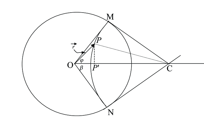
Figure 3: The outer circle is the intersection of the plane OMN with the 2-sphere boundary of the Poincaré ball. The geodesic connecting M to N is a circle whose centre is at C, and it intersects the boundary orthogonally at points M and N.

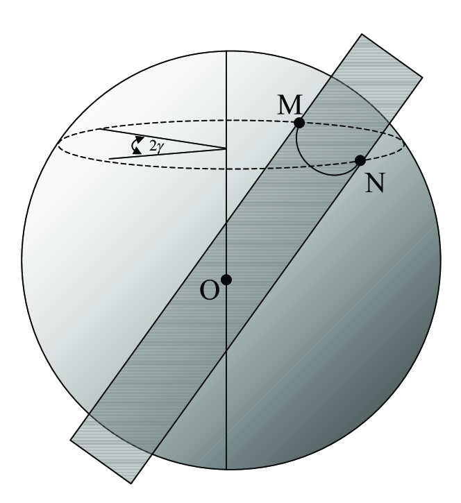
Figure 4: The intersection of the plane OMN with the Poincaré ball. A deficit angle of $2\gamma$ is cut out as shown.

To calculate the geodesic length, we parametrize the above geodesics (45) and (47) by

$$\sinh\chi=\sqrt{\frac{a^{{}^{\prime^{2}}}+\varsigma^{2}}{1-a^{{}^{\prime^{2}}}}},\text{ \ }\cos\theta=\cos\theta_{0}\sqrt{\frac{1+\varsigma^{2}}{a^{\prime^{2}}+\varsigma^{2}}},\text{ \ }\cos\varphi=b\cos\theta_{0}\sqrt{\frac{1+\varsigma^{2}}{a^{\prime^{2}}-1+(\varsigma^{2}+1)\sin^{2}\theta_{0}}}$$ (48)

where $0\leq\varsigma\leq\infty,$ and then substitute (48) into

$${\cal L}=\int\sqrt{\stackrel{{\scriptstyle\cdot}}{{\chi}}^{2}+\sinh^{2}\chi(\stackrel{{\scriptstyle\cdot}}{{\theta}}^{2}+\stackrel{{\scriptstyle\cdot}}{{\varphi}}^{2}\sin^{2}\theta)}d\varsigma$$ (49)

where the over-dot means differentiation with respect to the parameter $\varsigma.$ After integration over $\varsigma$, we obtain

$${\cal L}=2\ln\{\sinh\chi\sin\theta_{0}\sin\varphi+\sqrt{1+\sinh^{2}\chi\sin^{2}\theta_{0}\sin^{2}\varphi}\}$$ (50)

for the geodesic length between  the points $M$ and $N$. In the limit of $R\rightarrow 1$ or $\varepsilon\rightarrow 0$ this becomes

$${\cal L}=2\ln(\frac{2}{\varepsilon}\sin\theta_{0}\sin\varphi)$$ (51)

4.3 Conformal Field Theory Description of the Vortex Structure

We want to replace the vortex by a geometrical structure in the spacetime. We have seen in the preceding section that the metric is that of (4) with a deficit angle $2\gamma$. Then the constant time hypersurface in (42) is a Poincaré ball with a wedge cut from it that runs from $\theta=0$ to $\theta=\pi$. In any plane orthogonal to the $z$-axis, we have a wedge with angle $2\gamma$ with its boundary edges identified.

From (42) the boundary of AdS${}_{4\text{ }}$is ${\mathbf{R}\times S}^{2}$. Any closed curve on this boundary could be parametrized as $(t(\sigma),\theta(\sigma),\varphi(\sigma)),$ where the range of $\sigma$ is taken $0\leq\sigma\leq 2\pi.$ Now let us take any two points on the constant time boundary, i.e. on the sphere at the same polar angle $\theta_{0}$ with radius very close to the radius of boundary of Poincaré ball and opposite sign azimuth angles. In this case, where $t$, $\theta$ are constant, one can take the parameter $\sigma$ to be the same as $\varphi.$ Some of the geodesics passing through the two points which correspond to different values of $\sigma$ (or $\varphi$) intersect the edge of the wedge and some other do not.

Following ref. [14], we take coordinate systems $C_{1\text{ }}$ and $C_{2}$. In the first coordinate system, $C_{1}$, we take the range of deficit angle from $\pi-\gamma$ to $\pi+\gamma$, so the range of variation of polar coordinate $\varphi$ is $0\leq\varphi\leq\pi-\gamma,$ $\pi+\gamma\leq\varphi\leq 2\pi$. In the second coordinate system $C_{2}$, we take the deficit angle to be from $-\gamma$ to $+\gamma$. In this case the actual value of $\varphi$ changes between $\gamma$ and $2\pi-\gamma$.

When one increases the value of $\varphi$ from zero to some specific value, there exists an angle $\varphi_{c}$ for which the logarithmic derivative of the correlation function has a discontinuity. The reason is as follows.  It is a simple matter to see that the geodesics which intersect the identification in $C_{1\text{ }}$coordinate system do not intersect the identification in $C_{2\text{ }}$coordinate system and vice-versa. Hence in evaluating the length of the geodesics between two points which intersect the wedge of $C_{1},$ it is convenient to transform to $C_{2}$ coordinates. The effect of this is just to add a constant $\pm\gamma$ to the polar coordinate $\varphi$ of $C_{1}$ depending to its sign – $+\gamma$ for positive $\varphi$ and $-\gamma$ for negative $\varphi$. One can easily find that if the angle $\varphi$ is less than the critical polar angle , namely $\varphi_{c}=\frac{\pi-\gamma}{2}$, then the geodesics do not pass through the wedge $2\gamma.$ In this case, the length of geodesics should be computed in $C_{1}$, which is equal to (51). On the other hand, if the angle $\varphi$ is greater than the critical value $\varphi_{c}$, then the geodesics intersect the edges of the wedge and we must use the coordinate system $C_{2}$, which the length of geodesic is given by replacing $\varphi\rightarrow\varphi+\gamma$ in (51).

Hence there will be a discontinuity in the logarithmic derivative of the correlation function just in the neighborhood of $\varphi_{c}.$ The amount of this discontinuity is

$$K=\frac{1}{<{\cal OO}>}\frac{d<{\cal OO}>}{d\sigma}(\sigma_{c+})-\frac{1}{<{\cal OO}>}\frac{d<{\cal OO}>}{d\sigma}(\sigma_{c-})=2\Delta\frac{\partial\varphi(\sigma_{c})}{\partial\sigma}\tan\frac{\gamma}{2}$$ (52)

where as mentioned above, $\frac{\partial\varphi(\sigma_{c})}{\partial\sigma}$ is some constant $C_{0}$, which could be set equal to $1$. Although the correlation function depends on $\theta_{0}$, the magnitude of the kink is independent of this quantity. We will return to this point later.

5 The Vortex Mass in AdS₄

In this section we compute the mass of the vortex, which is equivalent to the mass of AdS₄ with a deficit angle of $\ 2\gamma$.

We choose a two-dimensional manifold ${\cal B}$, which is the boundary of the Poincaré ball at $R=l$, or $r=r_{0}\rightarrow\infty$. The boundary stress tensor is

$$T^{\mu\nu}=\frac{1}{8\pi}\{\Theta^{\mu\nu}-\Theta\gamma^{\mu\nu}+\frac{2}{\sqrt{-\gamma}}\frac{\delta I_{ct}}{\delta\gamma_{\mu\nu}}\}$$ (53)

where $\gamma^{\mu\nu\text{ }}$is the induced metric on the boundary of AdS₄ ($\partial$AdS₄), located at $R=l$ with extrinsic curvature $\Theta^{\mu\nu}$. The counterterm action $I_{ct}$ is given by [23]

$$I_{ct}=\frac{1}{4\pi l}\int_{\partial AdS_{4}}d^{3}x\sqrt{-\gamma}(1+\frac{l^{2}}{4}{\cal R})$$ (54)

which, when added to the usual Einstein-Hilbert action of AdS-gravity, removes its divergences at $r\rightarrow\infty$.

The mass is given by [24]

$$M=\frac{1}{8\pi}\int_{{\cal B}}d^{2}x\sqrt{\sigma}T_{\mu\nu}u^{\mu}\xi^{\nu}$$ (55)

where $u^{\mu}$ is the timelike normal unit vector to the boundary ${\cal B}$ with the metric $\sigma^{ab}$, and defines the local arrow of time on the boundary of AdS${}_{4\text{ }}$. $\xi^{\nu}$ is the time-like Killing vector of AdS₄.

The deficit angle in the AdS${}_{4\text{ }}$space yields a singular structure in the induced Ricci scalar of the boundary ${\cal B}$. These conical singularity structures are due to the identification of the edges of the wedge at the points $\theta=0$ and $\theta=\pi$ on the ${\cal B}$. To handle these singularities,  we replace the boundary ${\cal B}$ with a sequence of  regular manifolds [25, 26]. The first and second regular manifolds $\widetilde{{\cal M}_{\gamma}^{(0)}}$, $\widetilde{{\cal M}_{\gamma}^{(\pi)}}$ are regulated manifolds corresponding to the ${\cal M}_{\gamma}^{(0)}$, ${\cal M}_{\gamma}^{(\pi)}$ which are two dimensional spaces with the topology of a cone in the neighborhood of the poles of the boundary ${\cal B}$. The third manifold is ${\cal B}/{\cal(}{\cal M}_{\gamma}^{(0)}\otimes$ ${\cal M}_{\gamma}^{(\pi)})$, which can be smoothly matched to the other two. On the manifolds ${\cal M}_{\gamma}^{(0)}$, ${\cal M}_{\gamma}^{(\pi)}$,  the metric is,

$$r_{0}^{2}(d\theta^{2}+\theta^{2}d\varphi^{2})$$ (56)

where the polar coordinate $\varphi$ is restricted to the interval $[0,2(\pi-\gamma)].$ We take the following form of the metric for the regular manifolds  $\widetilde{{\cal M}_{\gamma}^{(0)}}$, $\widetilde{{\cal M}_{\gamma}^{(\pi)}}$,

$$r_{0}^{2}\{(1-\frac{\gamma}{\pi})^{2}+\frac{\gamma}{\pi}(\frac{\gamma}{\pi}-2)[\frac{\partial f(\theta,a)}{\partial\theta}]^{2}\}d\theta^{2}+r_{0}^{2}\theta^{2}d\varphi^{2}$$ (57)

In the above equation, $f(\theta,a)$ is a function which is introduced to smooth off the tips of the cones, and is subject to the following conditions ,

$$\lim_{a\rightarrow 0}f(\theta,a)=\theta,\text{ }\lim_{a\rightarrow 0}\text{ }\frac{\partial f(\theta,a)}{\partial\theta}=0\text{\ }$$ (58)

where $a$ is the regulator parameter. By choosing an appropriate function form of $\ f(\theta,a)$ [26], it is easy to show that the Ricci scalar ${\cal R}_{\gamma}$ of the boundary ${\cal B}$ with conical singularities at $\theta=0$  and $\theta=\pi$ is

$${\cal R}_{\gamma}={\cal R}+\frac{2\gamma}{\pi-\gamma}\frac{1}{r_{0}^{2}}\{\delta(\theta)+\delta(\pi-\theta)\}$$ (59)

In the above relation, ${\cal R}$ is the Ricci scalar of the manifold ${\cal B}/{\cal(}{\cal M}_{\gamma}^{(0)}\otimes$ ${\cal M}_{\gamma}^{(\pi)})$ and the Dirac delta function is subject to the following normalization,

$$\int\theta\delta(\theta)d\theta=1$$ (60)

Putting these together, (55) gives for the mass of AdS₄, containing a wedge ,

$$M=\frac{\gamma}{2\pi}r_{0}$$ (61)

in agreement with (37) in the limit that the thickness $\rho_{0}$ of the string is negligible.

6 Conclusion

We have solved the Nielsen-Olesen equations in an AdS₄ background, and found that the Higgs and gauge fields are axially symmetric, with non-zero winding number. Our solution in the limit of  large $l$ (small cosmological constant) reduces to the well known flat-space [15], and has well-defined characteristic lengths $\lambda$ and $\beta$ outside of which the fields exponentially approach their asymptotic values. The solution (to leading order in the gravitational coupling) induces a deficit angle in AdS₄. We find these results compelling enough to interpret our solution as a vortex.

The holographic detection of a Nielsen-Olesen vortex is now obtained by comparing eqs. (52) and (61). Although the total mass of the vortex is infinite, the mass per unit length is finite, and we can relate this to the kink (52) in the correlation function computed above. Since the kink depends only on the deficit angle $\gamma$, therefore for a fixed $\gamma,$ the kink is constant. On the other hand mass density also depends only on $\gamma$, and therefore one could interpret the value of the kink as the mass per unit length. From (61), the mass per unit length is equal to $\mu=\frac{M}{2r_{0}}=\frac{\gamma}{4\pi}$,  and we obtain

$$\frac{M}{2r_{0}}=\frac{1}{2\pi}\arctan\left(\frac{K}{2C_{0}\Delta}\right)$$ (62)

for the relationship between the vortex mass density and the kink in the CFT correlation function.

The winding number of the vortex also has a holographic description.  The field $\Phi$ in (5) has the same phase as its limiting field at the boundary of AdS₄ . Consequently the winding number of the vortex is given by the line-integral of the corresponding one-point function about any loop which encloses $\theta=0$ on the $(2+1)$-dimensional boundary.

Of course another holographic effect of the vortex is to induce conical singularities in the boundary at $\theta=0,\pi$ . The holographic interpretation is that the boundary CFT is formulated on a space that has a conical deficit.  However note that the presence of such singularities need not imply the presence of a kink in the correlation function.  It is this kink – present at any latitude of the boundary spacetime – that signals the presence of a vortex.

Our results are commensurate with those of ref. [14]:  non-local properties of the two point correlation function in the dual conformal field theory (the kink, in this case) probe the interior of the bulk geometry.  We have considered only the two point function of the operator on the boundary which is dual to the scalar field $\Phi$ in the Lagrangian (3).  As we have seen, this correlation function is related to the mass density of the vortex. An understanding of the role of the other two, three and four points correlation functions remains to be carried out, along with a more detailed study of the vortex itself, including obtaining a holographic description of its interior structure, and of threading it through a black hole. Work on these problems is in progress.

Acknowledgments

This work was supported by the Natural Sciences and Engineering Research Council of Canada.

References

- [1] J. Maldacena, Adv. Theor. Math. Phys. 2, 231 (1998), hep-th/9711200.
- [2] E. Witten, Adv. Theor. Math. Phys. 2, 253 (1998), hep-th/9802150.
- [3] K. Sfetsos, K. Skenderis, Nucl. Phys. B517, 179 (1998) .
- [4] D.Z. Freedman, S.D. Mathur, A. Matusis, L. Rastelli, Nucl. Phys. B546, 96 (1999), hep-th/9804058.
- [5] S. S. Gubser, I.R. Klebanov, A. M. Polyakov, Phys. Lett. B428, 105 (1998), hep-th/9802109.
- [6] W. Muck, K.S. Viswanathan, Phys. Rev. D58, 041901 (1998), hep-th/9804035.
- [7] M. Henningson, K. Sfetsos, Phys. Lett. B431, 63 (1998), hep-th/9803251.
- [8] A.M. Ghezelbash, K. Kaviani, S. Parvizi, A.H. Fatollahi, Phys. Lett. B435, 291 (1998), hep-th/9805162.
- [9] H. Liu, A.A. Tseytlin, Nucl. Phys. B533, 88 (1998), hep-th/9804083.
- [10] T. Banks, M.B. Green, JHEP 9805, 002 (1998), hep-th/9804170.
- [11] G. Chalmers, H. Nastase, K. Schalm, R. Siebelink, Nucl. Phys. B540, 247 (1999), hep-th/9805105.
- [12] V. Balasubramanian, P. Kraus, A. Lawrence, S.P. Trivedi, Phys. Rev. D59, 104021 (1999), hep-th/9808017.
- [13] U.H. Danielsson, E. Keski-Vakkuri, M. Kruczenski, JHEP 01, 002 (1999), hep-th/9812007.
- [14] V. Balasubramanian, S.F. Ross, Phys. Rev. D61, 044007 (2000), hep-th/9906226.
- [15] H.B. Nielsen, P. Olesen, Nucl. Phys. B61, 45 (1973).
- [16] A. Achucarro, R. Gregory, K. Kuijken, Phys. Rev. D52, 5729 (1995), gr-qc/9505039.
- [17] S. Weinberg, Quantum Field Theory III, ch 28, Cambridge University Press, (2000).
- [18] Y. Koma, M. Koma, D. Ebert, H. Toki, hep-th/0108138.
- [19] M. Abramovitz, I. Stegun, “Handbook of Mathematical Functions : With Formulas, Graphs, and Mathematical Tables”, New York : Academic Press, (1975).
- [20] E.B. Bogomolnyi, Yad. Fiz. 24 861 (1976) [Sov. J. Nucl. Phys. 24, 449, (1976)].
- [21] J.L. Synge, ”Relativity: The General Theory”, Amsterdam: North Holland, (1960).
- [22] J. Louko, D. Marolf, S.F. Ross, Phys. Rev. D62, 044041 (2000), hep-th/0002111.
- [23] R.B. Mann, Phys. Rev. D60, 104047 (1999); R. Emparan, C.V. Johnson, R. Meyers, Phys. Rev. D60, 104001 (1999); M. Hennigson, K. Skenderis, JHEP 9807 023 (1998) ; S.Y. Hyun, W.T. Kim, J. Lee, Phys. Rev. D59 084020 (1999) ; V. Balasubramanian, P. Kraus, Commun. Math. Phys. 208, 413 (1999).
- [24] J.D. Brown, J. Creighton, R.B. Mann, Phys. Rev. D50, 6394 (1994).
- [25] R.B. Mann, S.N. Solodukhin, Phys. Rev. D54, 3932 (1996), hep-th/9604118.
- [26] D.V. Fursaev, S.N. Solodukhin, Phys. Rev. D52, 2133 (1995), hep-th/9501127.