Bulk effects in the cosmological dynamics of brane-world scenarios

Abstract

In this paper we deal with the cosmological dynamics of Randall-Sundrum brane-world type scenarios in which the five-dimensional Weyl tensor has a non-vanishing projection onto the three-brane where matter fields are confined. Using dynamical systems techniques, we study how the state space of Friedmann-Lemaître-Robertson-Walker (FLRW) and Bianchi type I cosmological models is affected by the bulk Weyl tensor, focusing in the differences that appear with respect to general relativity and also Randall-Sundrum cosmological scenarios without the Weyl tensor contribution.

]

I Introduction

Recently, Randall and Sundrum have shown that for non-factorizable geometries in five dimensions the zero-mode of the Kaluza-Klein dimensional reduction can be localized in a four-dimensional submanifold where Newtonian gravity is effectively reproduced at large distances [1]. The picture coming out is one with all matter and gauge fields, excepting gravity, confined in a three-brane embedded in a five-dimensional spacetime with ${\mathbb{Z}}_{2}$ symmetry. This scenario was motivated by orbifold compactification of higher dimensional string theories. In particular by the dimensional reduction of eleven-dimensional supergravity in ${\mathbb{R}}^{10}\times S^{1}/{\mathbb{Z}}_{2}$ introduced by Ho$\check{\mbox{r}}$ava and Witten[2]. The cosmological implications of the Ho$\check{\mbox{r}}$ava-Witten theory have been analyzed in [3]. The actual relevance of this type of scenarios is that they provide an alternative framework to investigate new solutions to the hierarchy and cosmological constant problems.

Gravity on the brane can be described by the Einstein equations modified by two additional terms, one quadratic in the matter variables and the second one being the “electric” part of the five-dimensional Weyl tensor [4, 5, 6, 7]. In a previous work [8] we studied the whole dynamics of the Friedmann-Lemaître-Robertson-Walker (FLRW) and the Bianchi type I and V cosmological models taking into account only the effects produced by the first type of corrections. In that paper we found new critical points corresponding to the Bin$\acute{\mbox{e}}$truy-Deffayet-Langlois (BDL) models [4], representing the dynamics at very high energies, where the extra-dimension effects become dominant. The presence of these models seems to be a generic feature of the state space of more general cosmological models. Moreover, we saw that the state space presents new bifurcations and how the dynamical character of some of the critical points changes with respect to the general-relativistic case. Finally, we showed that for models satisfying all the ordinary energy conditions and causality requirements the anisotropy is negligible near the initial singularity. On the other hand, for late times the anisotropy is diluted as in general relativity (GR) but now there are intermediate stages in which the shear contribution grows.

Here, we will complete the analysis done in [8] (hereafter Paper I) studying the effects of the five-dimensional Weyl tensor on FLRW and Bianchi type I cosmological models. In the case of FLRW models this study will be completely general whereas in the Bianchi type I case we will neglect the Weyl tensor components for which the theory does not provide evolution equations. The paper is organized as follows. In Sec. II we briefly describe the geometric formulation of brane-world scenarios and the dynamical equations for FLRW and Bianchi type I cosmological models with a perfect-fluid type matter content. The dynamics of the FLRW and Bianchi type I cosmological models will be analyzed in Secs. III and IV respectively. We will finish with some concluding remarks in Sec. V. Through this paper we will follow the following notation: upper-case Latin letters denote coordinate indices in the bulk spacetime ($A,B,\ldots=0-4$) whereas lower-case Latin letters denote coordinate indices in the brane ($a,b,\ldots=0-3$). We use physical units in which $c=1$.

II Preliminaries

In what follows we introduce the geometric framework to analyze the brane-world scenario and the main assumptions we will adopt to study the FLRW and Bianchi type I cosmological models.

A Geometric formulation of brane-world scenarios

In Randall-Sundrum brane-world type scenarios matter fields are confined in a three-brane embedded in a five-dimensional spacetime (bulk). It is assumed that the metric of this spacetime, $g^{(5)}_{AB}$, obeys the Einstein equations with a negative cosmological constant $\Lambda_{(5)}$ (see [6, 7, 9])

$$G^{(5)}_{AB}=-\Lambda_{(5)}g^{(5)}_{AB}+\kappa^{2}_{(5)}\delta(\chi)\left[-\lambda\,g_{AB}+T_{AB}\right]\,,$$ (1)

where $G^{(5)}_{AB}$ denotes the Einstein tensor and $\kappa_{(5)}$ is the five-dimensional gravitational coupling constant. Moreover, $T_{AB}$ is the matter energy-momentum tensor and the Dirac delta function reflects the fact that matter is confined in the spacelike hypersurface $x^{4}\equiv\chi=0$, the three-brane, with induced metric $g_{AB}$ and tension $\lambda\,.$

From the Gauss-Codacci equations, the Israel junction conditions and the ${\mathbb{Z}}_{2}$ symmetry with respect to the three-brane, we can see [6, 7] that the effective Einstein equations on the brane are

$$G_{ab}=-\Lambda g_{ab}+\kappa^{2}T_{ab}+\kappa^{4}_{(5)}S_{ab}-E^{(5)}_{ab}\,,$$ (2)

where $G_{ab}$ is the Einstein tensor of the induced metric $g_{ab}\,.$ The four-dimensional gravitational constant $\kappa$ and the cosmological constant $\Lambda$ are given in terms of the fundamental constants in the bulk $(\kappa_{(5)},\Lambda_{(5)})$ and the brane tension $\lambda$. It is important to note that in order to recover conventional gravity on the brane $\lambda$ must be assumed to be positive. As one can observe, there are two corrections to the general-relativistic equations. The first one, denoted by the term $S_{ab}$, is quadratic in the matter energy-momentum tensor $T_{ab}$ ($T\equiv g^{ab}T_{ab}$)

$$S_{ab}=\textstyle{1\over 12}TT_{ab}-\textstyle{1\over 4}T_{a}{}^{c}T_{bc}+\textstyle{1\over 24}g_{ab}\left[3T^{cd}T_{cd}-T^{2}\right]\,.$$ (3)

The second correction, $E^{(5)}_{ab}$, correspond to the “electric” part of the five-dimensional Weyl tensor, $C^{(5)}_{ABCD}$, with respect to the normal, $n_{A}$ ($n^{A}n_{A}=1$), to the hypersurface $\chi=0$, that is

$\displaystyle E^{(5)}_{AB}=C^{(5)}_{ACBD}n^{C}n^{D}\,.$

From the modified Einstein equations (2) and the energy-momentum tensor conservation equations ($\nabla_{a}T^{a}{}_{b}=0$) we get a constraint on $S_{ab}$ and $E^{(5)}_{ab}$

$$\nabla^{a}(E^{(5)}_{ab}-\kappa^{4}_{(5)}S_{ab})=0\,.$$ (4)

Following [9], it is useful to decompose $E^{(5)}_{ab}$ with respect to any timelike observers $u$ ($u^{a}u_{a}=-1$) in a scalar part, ${\cal U}$, a vector part, ${\cal Q}_{a}$, and a tensorial part ${\cal P}_{ab}$, in such a way that $E^{(5)}_{ab}$ can be written as

$$E^{(5)}_{ab}=-\left(\frac{\kappa_{(5)}}{\kappa}\right)^{4}\left[(u_{a}u_{b}+\textstyle{1\over 3}h_{ab}){\cal U}+2u_{(a}{\cal Q}_{b)}+{\cal P}_{ab}\right]\,,$$ (5)

where the following properties hold

$\displaystyle{\cal Q}_{a}u^{a}=0\,,~{}~{}~{}{\cal P}_{(ab)}={\cal P}_{ab}\,,~{}~{}{\cal P}^{a}{}_{a}=0\,,~{}~{}{\cal P}_{ab}u^{b}=0\,.$

That is, ${\cal Q}_{a}$ is a spatial vector and ${\cal P}_{ab}$ is a spatial, symmetric and trace-free tensor. The scalar term has the same form as the energy-momentum tensor of a radiation perfect fluid, and for this reason ${\cal U}$ was called “dark” energy density in [9]. Note that the constraint (4) provides evolution equations for ${\cal U}$ and ${\cal Q}_{a}$, but not for ${\cal P}_{ab}$ (see [9]).

B Cosmological dynamics on the brane

Throughout this paper we will describe matter by a perfect fluid

$\displaystyle T_{ab}=(\rho+p)u_{a}u_{b}+pg_{ab}\,,$

where $u$, $\rho$ and $p$ are the unit fluid velocity of matter, the energy density and the pressure of the matter fluid respectively. We will also assume a linear barotropic equation of state for the fluid

$$p=(\gamma-1)\rho\,.$$ (6)

The weak energy condition (see, e.g., [10]) imposes the restriction $\rho\geq 0$ and from causality requirements we have that the parameter $\gamma\in[0,2]$.

In this paper we deal with non-tilted homogeneous cosmological models on the brane, i.e. we are assuming that the fluid velocity is orthogonal to the hypersurfaces of homogeneity. Then, it is convenient to make the splitting (5) with respect to the fluid velocity. In particular we will consider: (i) The FLRW models, with metric tensor given by

$\displaystyle\mbox{ds}^{2}=-dt^{2}+a^{2}(t)\left[dr^{2}+\Sigma^{2}_{k}(r)(d\theta^{2}+\sin^{2}\theta d\varphi^{2})\right]\,,$

where $a(t)$ is the scale factor, $k$ is the curvature parameter, and

$\displaystyle\Sigma_{k}(r)=\left\{\begin{array}[]{ll}\sin r&\mbox{for $k=1$}\,,\\ r&\mbox{for $k=0$}\,,\\ \sinh r&\mbox{for $k=-1$}\,;\end{array}\right.$

and (ii) Bianchi type I models, whose line element can be written as

$$\mbox{ds}^{2}=-dt^{2}+\sum_{\alpha=1}^{3}A^{2}_{\alpha}(t)(dx^{\alpha})^{2}\,.$$ (7)

Then, in both cases the fluid velocity is $\vec{\mbox{\boldmath$u$}}=\mbox{\boldmath$\partial$}/\mbox{\boldmath$\partial t$}\,.$ We will not consider Bianchi type V models as we did in Paper I because, as we showed there, their main dynamical features are a combination of those of the FLRW and Bianchi type I models.

Taking into account these assumptions and the effective Einstein’s equations (2), the consequences of having a FLRW model on the brane are

$\displaystyle{\cal Q}_{a}={\cal P}_{ab}=0\,,$

and this, through the constraint (4), further implies

$$D_{a}{\cal U}=0~{}\Leftrightarrow~{}{\cal U}={\cal U}(t)\,,$$ (8)

where $D_{a}$ denotes the covariant derivative associated with the induced metric on the hypersurfaces of homogeneity ($h_{ab}\equiv g_{ab}+u_{a}u_{b}$). Instead, in the case of Bianchi type I we get ${\cal Q}_{a}=0$ but we do not get any restriction on ${\cal P}_{ab}\,.$ Since there is no way of fixing the dynamics of this tensor we will study the particular case in which it is zero. Then, also the condition (8) follows.

The key equation to describe the dynamics of these models is the Friedmann equation, which determines the expansion of the universe, or in other words, the Hubble function: $3H\equiv\nabla_{a}u^{a}\,.$ The general expression of this equation in the case of homogeneous cosmological models is

$$H^{2}=\frac{1}{3}\kappa^{2}\rho\left(1+\frac{\rho}{2\lambda}\right)-\frac{1}{6}{}^{3}R+\frac{1}{3}\sigma^{2}+\frac{1}{3}\Lambda+\frac{2{\cal U}}{\lambda\kappa^{2}}\,,$$ (9)

where ${}^{3}R$ is the scalar curvature of the hypersurfaces orthogonal to the fluid flow and $2\sigma^{2}\equiv\sigma^{ab}\sigma_{ab}$ is the shear scalar ($\sigma_{ab}\equiv h_{a}{}^{c}h_{b}{}^{d}\nabla_{(c}u_{d)}-Hh_{ab}$). We consider only the case of a positive fourd-dimensional cosmological constant, i.e. $\Lambda\geq 0$. For Bianchi type I models ${}^{3}R$ vanishes whereas for FLRW models it is given by ${}^{3}R=6ka^{-2}(t)\,.$ On the other hand, the shear vanishes for FLRW models and for Bianchi type I models the evolution of the shear scalar is

$\displaystyle(\sigma^{2})^{\cdot}=-6H\sigma^{2}\,.$

In both cases the evolution equation for ${\cal U}$ is [9]

$\displaystyle\dot{\cal U}=-4H{\cal U}\,,$

and, from the energy-momentum conservation equation, the evolution of $\rho$ is simply

$$\dot{\rho}=-3\gamma H\rho\,.$$ (10)

Finally, an important quantity in the dynamical study will be the deceleration parameter $q$, defined by

$$\dot{H}\equiv-(1+q)H^{2}\,,$$ (11)

where $\dot{H}$ is found to be

$$\dot{H} = -H^{2}-\frac{3\gamma-2}{6}\kappa^{2}\rho\left[1+\frac{3\gamma-1}{3\gamma-2}\frac{\rho}{\lambda}\right]-\frac{2}{3}\sigma^{2}$$ (13)

$$+\frac{1}{3}\Lambda-\frac{2{\cal U}}{\lambda\kappa^{2}}\,,$$

which is the modified Raychaudhuri equation.

III Dynamics of the FLRW models

In Paper I we studied the dynamics of the FLRW cosmological models in a brane-world scenario in which the effects of the extra dimensions are only due to the term quadratic in the matter sources, $S_{ab}$ [see Eq. (2)]. Now, we will add the contribution of $E^{(5)}_{ab}\,,$ which, as we have seen above, only contains the scalar part ${\cal U}\,.$ In order to study the dynamics of these models we will closely follow the analysis carried out in Paper I. This procedure is based on the introduction of new variables which describe the dynamics in such a way that the state space is a compact space (see [11, 12] for details on the techniques of dynamical systems analysis). To carry out this study we have to consider four differentiated cases according to the signs of ${}^{3}R$ and ${\cal U}$: (A) ${\cal U}\geq 0$ and ${}^{3}R\leq 0$; (B) ${\cal U}\geq 0$ and ${}^{3}R\geq 0$; (C) ${\cal U}\leq 0$ and ${}^{3}R\leq 0$; (D) ${\cal U}\leq 0$ and ${}^{3}R\geq 0$.

A Case ${\cal U}\geq 0$ and ${}^{3}R\leq 0$

The state space in this case can be described by the dimensionless general-relativistic variables

$$\Omega_{\rho}\equiv\frac{\kappa^{2}\rho}{3H^{2}}\,,~{}~{}\Omega_{k}\equiv-\frac{{}^{3}R}{6H^{2}}\,,~{}~{}\Omega_{\Lambda}\equiv\frac{\Lambda}{3H^{2}}\,,$$ (14)

and the following new variables

$$\Omega_{\lambda}\equiv\frac{\kappa^{2}\rho^{2}}{6\lambda H^{2}}\,,~{}~{}\Omega_{\cal U}\equiv\frac{2{\cal U}}{\lambda\kappa^{2}H^{2}}\,.$$ (15)

Here $\Omega_{\rho}$ is the ordinary density parameter and $\Omega_{k}$, $\Omega_{\Lambda}$, $\Omega_{\lambda}$, and $\Omega_{\cal U}$ are the fractional contributions of the curvature, cosmological constant, brane tension, and the dark radiation energy, respectively, to the universe expansion (9). In fact, the Friedmann equation (9) becomes

$\displaystyle\Omega_{\rho}+\Omega_{k}+\Omega_{\Lambda}+\Omega_{\lambda}+\Omega_{\cal U}=1\,.$

Since these terms are non-negative they must belong to the interval $[0,1]$ and hence, the variables $\mbox{\boldmath$\Omega$}=(\Omega_{\rho},\Omega_{k},\Omega_{\Lambda},\Omega_{\lambda},\Omega_{\cal U})$ define a compact state space. Introducing the time derivative $|H|^{-1}d/dt$, which we will denote by a prime, the evolution equation for $H$ [Eq. (11)] will decouple from the equations for $\Omega$. Then, the set of equations describing the dynamics is given by

$$\Omega^{\prime}_{\rho} = \epsilon[2(1+q)-3\gamma]\Omega_{\rho}\,,$$ (16)

$$\Omega^{\prime}_{k} = 2\epsilon q\Omega_{k}\,,$$ (17)

$$\Omega^{\prime}_{\Lambda} = 2\epsilon(1+q)\Omega_{\Lambda}\,,$$ (18)

$$\Omega^{\prime}_{\lambda} = 2\epsilon(1+q-3\gamma)\Omega_{\lambda}\,,$$ (19)

$$\Omega^{\prime}_{\cal U} = 2\epsilon(q-1)\Omega_{\cal U}\,,$$ (20)

where $q$ is

$\displaystyle q=\frac{3\gamma-2}{2}\Omega_{\rho}-\Omega_{\Lambda}+(3\gamma-1)\Omega_{\lambda}+\Omega_{\cal U}\,,$

and $\epsilon$ is the sign of $H\,.$ As is clear, for $\epsilon=1$ the model will be in expansion, and for $\epsilon=-1$ it will be in contraction.

The critical points of the dynamical system (16)-(20), their coordinates in the state space and their eigenvalues are given in the following table [13]

Model	Coordinates	Eigenvalues
$\mbox{F}_{\epsilon}$	$(1,0,0,0,0)$	$\epsilon(3\gamma-2,3\gamma-2,3\gamma,-3\gamma,3\gamma-4)$
$\mbox{M}_{\epsilon}$	$(0,1,0,0,0)$	$\epsilon(-(3\gamma-2),0,2,-2(3\gamma-1),-2)$
$\mbox{dS}_{\epsilon}$	$(0,0,1,0,0)$	$-\epsilon(3\gamma,2,2,6\gamma,4)$
$\mbox{m}_{\epsilon}$	$(0,0,0,1,0)$	$2\epsilon(\textstyle{3\gamma\over 2},(3\gamma-1),3\gamma,3\gamma-1,3\gamma-2)$
$\mbox{R}_{\epsilon}$	$(0,0,0,0,1)$	$\epsilon(-(3\gamma-4),2,4,-2(3\gamma-2),2)$

We have five hyperbolic critical points: the flat FLRW models (F), $k=\Lambda=\lambda^{-1}={\cal U}=0$ and $a(t)=t^{2/(3\gamma)}$; the Milne universe (M), $\rho=\Lambda={\cal U}=0\,,$ $k=-1$ and $a(t)=t$; the de Sitter model (dS), $k=\rho={\cal U}=0$ and $a(t)=\exp(\sqrt{\Lambda/3}\,t)$; the non-general-relativistic BDL model (m) [4, 5, 14], found through a limiting process to be $a(t)=t^{1/(3\gamma)}$ (see Paper I for more details); and a model (R) with the metric of a flat radiation FLRW model, $a(t)=t^{1/2}$, but characterized by $\rho=k=\Lambda=\lambda^{-1}=0$.

B Case ${\cal U}\geq 0$ and ${}^{3}R\geq 0$

Here we can follow the study corresponding to the non-negative scalar curvature case in Paper I. Then, we will consider the variables $\mbox{\boldmath$\tilde{\Omega}$}\equiv(Q,\tilde{\Omega}_{\rho},\tilde{\Omega}_{\Lambda},\tilde{\Omega}_{\lambda},\tilde{\Omega}_{\cal U})$, where Q is

$\displaystyle Q\equiv\frac{H}{D}\,,~{}~{}~{}D^{2}\equiv H^{2}+\textstyle{1\over 6}{}^{3}R\,.$

and the variables with tilde are the analogues of those in (14) and (15) but normalized with respect to $D$ instead of $H$. Then, the Friedmann equation (9) is now

$$\tilde{\Omega}_{\rho}+\tilde{\Omega}_{\Lambda}+\tilde{\Omega}_{\lambda}+\tilde{\Omega}_{\cal U}=1\,.$$ (21)

Taking into account that $q$ is now given by

$\displaystyle 1+qQ^{2}=\textstyle{{3\gamma}\over 2}(\tilde{\Omega}_{\rho}+2\tilde{\Omega}_{\lambda})+2\tilde{\Omega}_{\cal U}\,,$

and using the time derivative ${}^{\prime}\equiv D^{-1}d/dt\,,$ the dynamical equations for $\tilde{\Omega}$ are decoupled from $D$ and are given by

$$Q^{\prime} = -qQ^{2}(1-Q^{2})\,,$$

$$\tilde{\Omega}^{\prime}_{\rho} = [2(1+qQ^{2})-3\gamma]Q\tilde{\Omega}_{\rho}\,,$$

$$\tilde{\Omega}^{\prime}_{\Lambda} = 2(1+qQ^{2})Q\tilde{\Omega}_{\Lambda}\,,$$

$$\tilde{\Omega}^{\prime}_{\lambda} = 2[1+qQ^{2}-3\gamma]Q\tilde{\Omega}_{\lambda}\,,$$

$$\tilde{\Omega}^{\prime}_{\cal U} = -2(1-qQ^{2})Q\tilde{\Omega}_{\cal U}\,.$$

The critical points of this dynamical system, as well as their coordinates and eigenvalues are [13]

Model	Coordinates	Eigenvalues
$\mbox{F}_{\epsilon}$	$(\epsilon,1,0,0,0)$	$\epsilon(3\gamma-2,3\gamma,3\gamma,-3\gamma,3\gamma-4)$
$\mbox{dS}_{\epsilon}$	$(\epsilon,0,1,0,0)$	$-\epsilon(2,3\gamma,0,6\gamma,4)$
E	$(0,\tilde{\Omega}^{\ast}_{\rho},\tilde{\Omega}^{\ast}_{\Lambda},\tilde{\Omega}^{\ast}_{\lambda},\tilde{\Omega}^{\ast}_{\cal U})$	$(0,\sqrt{\phi},0,-\sqrt{\phi},0)$
$\mbox{m}_{\epsilon}$	$(\epsilon,0,0,1,0)$	$2\epsilon(3\gamma-1,\textstyle{{3\gamma}\over 2},3\gamma,3\gamma,3\gamma-2)$
$\mbox{R}_{\epsilon}$	$(\epsilon,0,0,0,1)$	$\epsilon(2,-(3\gamma-4),4,-2(3\gamma-2),4)$

Here E denotes a infinite set of saddle points whose line element is that of the Einstein universe ($k=1$ and $H=0$). Their coordinates $\tilde{\Omega}^{\ast}$ satisfy (21) and

$$1-\frac{3\gamma}{2}(\tilde{\Omega}^{\ast}_{\rho}+2\tilde{\Omega}^{\ast}_{\lambda})-2\tilde{\Omega}^{\ast}_{\cal U}=0\,.$$ (22)

In the table above $\phi$ is given by

$\displaystyle\phi=\frac{3\gamma}{2}\left[\left(3\gamma-2\right)\tilde{\Omega}^{\ast}_{\rho}+4\left(3\gamma-1\right)\tilde{\Omega}^{\ast}_{\lambda}\right]+4\tilde{\Omega}^{\ast}_{\cal U}\,.$

From the relation (22) and the allowed values of the variables $\tilde{\Omega}$ one can show that $\phi$ is always positive for any $\gamma\,.$ In GR the Einstein universe appears for $\gamma\geq 2/3\,.$ In Paper I we showed that in brane-world scenarios without the contribution coming from the five-dimensional Weyl tensor it appears for $\gamma\geq 1/3\,.$ Now, considering also this contribution Eq. (22) shows that the Einstein universe appears for any value of $\gamma\,.$

C Case ${\cal U}\leq 0$ and ${}^{3}R\leq 0$

In this case we can get a compact state space by introducing the following set of dynamical variables $\mbox{\boldmath$\bar{\Omega}$}\equiv(Z,\bar{\Omega}_{\rho},\bar{\Omega}_{k},\bar{\Omega}_{\Lambda},\bar{\Omega}_{\lambda})$, where

$$Z\equiv\frac{H}{N}\,,~{}~{}N^{2}\equiv H^{2}-\frac{2{\cal U}}{\lambda\kappa^{2}}\,,$$ (23)

and the variables with a bar are like those in (14) and (15) but normalized with respect to $N$ instead of $H$. As before, the Friedmann equation (9) reduces to an expression in which all the terms are non-negative

$$\bar{\Omega}_{\rho}+\bar{\Omega}_{k}+\bar{\Omega}_{\Lambda}+\bar{\Omega}_{\lambda}=1\,,$$ (24)

whence it follows that all of them are smaller than $1\,.$ Using the time derivative ${}^{\prime}\equiv N^{-1}d/dt\,,$ in order to decouple the evolution of $N$ from the rest of variables, and taking into account the expression for $q$

$\displaystyle(q-1)Z^{2}=\textstyle{{3\gamma}\over 2}(\bar{\Omega}_{\rho}+2\bar{\Omega}_{\lambda})+\bar{\Omega}_{k}-2\,,$

the dynamical system for $\bar{\Omega}$ is

$$Z^{\prime} = -(q-1)Z^{2}(1-Z^{2})\,,$$

$$\bar{\Omega}^{\prime}_{\rho} = -[(3\gamma-4)-2(q-1)Z^{2}]Z\bar{\Omega}_{\rho}\,,$$

$$\bar{\Omega}^{\prime}_{k} = 2[1+(q-1)Z^{2}]Z\bar{\Omega}_{k}\,,$$

$$\bar{\Omega}^{\prime}_{\Lambda} = 2[2+(q-1)Z^{2}]Z\bar{\Omega}_{\Lambda}\,,$$

$$\bar{\Omega}^{\prime}_{\lambda} = -2[(3\gamma-2)-(q-1)Z^{2}]Z\bar{\Omega}_{\lambda}\,.$$

The critical points, their coordinates and eigenvalues are given in the table bellow [13]

Model	Coordinates	Eigenvalues
$\mbox{F}_{\epsilon}$	$(\epsilon,1,0,0,0)$	$\epsilon(3\gamma-4,3\gamma,3\gamma-2,3\gamma,-3\gamma)$
$\mbox{M}_{\epsilon}$	$(\epsilon,0,1,0,0)$	$\epsilon(-2,-(3\gamma-2),2,2,-2(3\gamma-1))$
$\mbox{dS}_{\epsilon}$	$(\epsilon,0,0,1,0)$	$-\epsilon(4,3\gamma,2,0,6\gamma)$
$\mbox{m}_{\epsilon}$	$(\epsilon,0,0,0,1)$	$2\epsilon(3\gamma-2,\textstyle{3\gamma\over 2},3\gamma-1,3\gamma,3\gamma)$
S	$(0,\bar{\Omega}^{\ast}_{\rho},\bar{\Omega}^{\ast}_{k},\bar{\Omega}^{\ast}_{\Lambda},\bar{\Omega}^{\ast}_{\lambda})$	$(0,\sqrt{\psi},0,0,-\sqrt{\psi})$

We find new critical points, denoted by S, representing static models with vanishing and negative spatial curvature, i.e. $H=0$ and $k=0,-1\,.$ Moreover $\bar{\Omega}^{\ast}_{\rho}\,,$ $\bar{\Omega}^{\ast}_{k}\,,$ $\bar{\Omega}^{\ast}_{\Lambda}\,,$ and $\bar{\Omega}^{\ast}_{\lambda}$ are real numbers satisfying (24) and the following relation

$$2-\bar{\Omega}^{\ast}_{k}-\frac{3\gamma}{2}(\bar{\Omega}^{\ast}_{\rho}+2\bar{\Omega}^{\ast}_{\lambda})=0\,.$$ (25)

The eigenvalues of S are given in terms of $\psi$:

$$\psi=\frac{3\gamma}{2}\left[(3\gamma-4)\bar{\Omega}^{\ast}_{\rho}+4(3\gamma-2)\bar{\Omega}^{\ast}_{\lambda}\right]-2\bar{\Omega}^{\ast}_{k}\,.$$ (26)

Eq. (25) implies that these static models (S) only appear for $\gamma\geq 2/3$. Furthermore $a\,,$ $\rho$ and ${\cal U}$ are constants, $(a^{\ast},\rho^{\ast},{\cal U}^{\ast})$, which must satisfy the following condition

$$-{\cal U}^{\ast}\geq\frac{\lambda\kappa^{2}}{2}\left(\frac{\Lambda}{3}-\frac{k}{a^{\ast^{2}}}\right)\,,$$ (27)

in order to have a positive energy density.

D Case ${\cal U}\leq 0$ and ${}^{3}R\geq 0$

This case is more involve since the Friedmann equation (9) has now two non-positive terms. Taking this into account we will consider the following dimensionless dynamical variables $\mbox{\boldmath$\hat{\Omega}$}=(W,\hat{\Omega}_{\rho},\hat{\Omega}_{\Lambda},\hat{\Omega}_{\lambda},\hat{\Omega}_{\cal U})$, where

$\displaystyle W\equiv\frac{H}{P}\,,~{}~{}~{}P^{2}\equiv H^{2}+\frac{1}{6}{}^{3}R-\frac{2{\cal U}}{\lambda\kappa^{2}}\,,$

$\hat{\Omega}_{\rho}\,,$ $\hat{\Omega}_{\Lambda}\,,$ $\hat{\Omega}_{\cal U}\,,$ and $\hat{\Omega}_{\lambda}$ are the analogous of those in (14) and (15) but normalized with $P$. It is important to note that $\hat{\Omega}_{\cal U}$ does not appear in the Friedmann equation (9), which now reads

$$\hat{\Omega}_{\rho}+\hat{\Omega}_{\Lambda}+\hat{\Omega}_{\lambda}=1\,,$$ (28)

but it will be needed to close the dynamical system. Moreover, in this case $\hat{\Omega}_{\cal U}$ is negative and from its definition it belongs to the interval $[-1,0]\,.$ Then, using the time derivative ${}^{\prime}\equiv P^{-1}d/dt$, and the expression for $q$

$\displaystyle 1+qW^{2}=\textstyle{{3\gamma}\over 2}(\hat{\Omega}_{\rho}+2\hat{\Omega}_{\lambda})+\hat{\Omega}_{\cal U}\,,$

the evolution equations for $\hat{\Omega}$ are

$$W^{\prime} = -[q(1-W^{2})+\hat{\Omega}_{\cal U}]W^{2}\,,$$ (29)

$$\hat{\Omega}^{\prime}_{\rho} = [2(1+qW^{2})-(2\hat{\Omega}_{\cal U}+3\gamma)]W\hat{\Omega}_{\rho}\,,$$ (30)

$$\hat{\Omega}^{\prime}_{\Lambda} = 2(1+qW^{2}-\hat{\Omega}_{\cal U})W\hat{\Omega}_{\Lambda}\,,$$ (31)

$$\hat{\Omega}^{\prime}_{\lambda} = 2[1+qW^{2}-(\hat{\Omega}_{\cal U}+3\gamma)]W\hat{\Omega}_{\lambda}\,,$$ (32)

$$\hat{\Omega}^{\prime}_{\cal U} = 2[qW^{2}-\hat{\Omega}_{\cal U}-1]W\hat{\Omega}_{\cal U}\,.$$ (33)

The critical points and their coordinates and eigenvalues are [13]

Model	Coordinates	Eigenvalues
$\mbox{F}_{\epsilon}$	$(\epsilon,1,0,0,0)$	$\epsilon(3\gamma-2,3\gamma,3\gamma,-3\gamma,3\gamma-4)$
$\mbox{dS}_{\epsilon}$	$(\epsilon,0,1,0,0)$	$-\epsilon(2,3\gamma,0,6\gamma,4)$
$\mbox{m}_{\epsilon}$	$(\epsilon,0,0,1,0)$	$2\epsilon(3\gamma-2,\textstyle{{3\gamma}\over 2},3\gamma,3\gamma,3\gamma-2)$
E	$(0,\hat{\Omega}^{\ast}_{\rho},\hat{\Omega}^{\ast}_{\Lambda},\hat{\Omega}^{\ast}_{\lambda},\hat{\Omega}^{\ast}_{\cal U})$	$(0,\sqrt{\varphi},0,-\sqrt{\varphi},0)$

where $\hat{\Omega}^{\ast}_{\rho}\,,$ $\hat{\Omega}^{\ast}_{\Lambda}\,,$ $\hat{\Omega}^{\ast}_{\lambda}\,,$ and $\hat{\Omega}^{\ast}_{\cal U}$ are real numbers satisfying (28) and

$\displaystyle\frac{3\gamma}{2}(\hat{\Omega}^{\ast}_{\rho}+2\hat{\Omega}^{\ast}_{\lambda})+\hat{\Omega}^{\ast}_{\cal U}-1=0\,.$

Now, the eigenvalues of the Einstein universe are determined by $\varphi$, which is given by

$\displaystyle\varphi=\frac{3\gamma}{2}\left[(3\gamma-2)\hat{\Omega}^{\ast}_{\rho}+4(3\gamma-1)\hat{\Omega}^{\ast}_{\lambda}\right]+4\hat{\Omega}^{\ast}_{\cal U}\,.$

In contrast to what happens in the state space sector analyzed in subsection III B the Einstein universe now appears for $\gamma\geq 1/3$, just when $\varphi$ starts being non-negative.

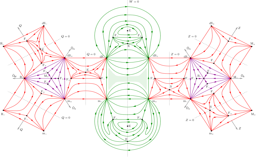
FIG. 1.: Full state space for FLRW models with $\gamma\in(\textstyle{2\over 3},\textstyle{4\over 3})$ .

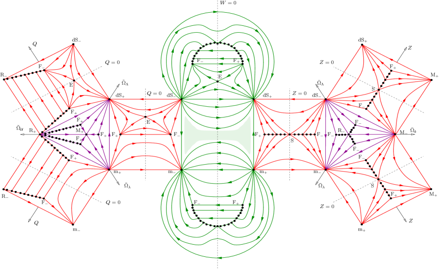
FIG. 2.: Full state space for FLRW models with $\gamma=\textstyle{4\over 3}$ .

E Qualitative analysis

Using the information obtained in the previous subsections we are going to describe qualitatively the full dynamics of FLRW in brane-world scenarios. To that end, we will construct and analyze the structure of the complete state space for these models. To start with, we need to know the dynamical character of the critical points. This can be deduced from the eigenvalues given above and summarized in the following table

Model	Dynamical character
	$0<\gamma<\textstyle{2\over 3}$	$\gamma=\textstyle{2\over 3}$	$\gamma>\textstyle{2\over 3}$
$\mbox{F}_{\pm}$	saddle	saddle	saddle
$\mbox{M}_{\pm}$	saddle	saddle	saddle
$\mbox{dS}_{+}$	attractor	attractor	attractor
$\mbox{dS}_{-}$	repeller	repeller	repeller
E	saddle	saddle	saddle
$\mbox{m}_{+}$	saddle	repeller	repeller
$\mbox{m}_{-}$	saddle	attractor	attractor
$\mbox{R}_{+}$	repeller	repeller	saddle
$\mbox{R}_{-}$	attractor	attractor	saddle
S	—	saddle	saddle

We can observe some changes with respect to GR and the analysis done for ${\cal U}=0$ (Paper I). For instance, the Milne universe is always a saddle point for ${\cal U}\neq 0$ whereas $\mbox{M}_{+}$ ($\mbox{M}_{-}$) is a repeller (attractor) for $\gamma\leq 2/3$ in GR and for $\gamma\leq 1/3$ in brane-world scenarios with ${\cal U}=0\,.$

The full state space for the FLRW models is four-dimensional, due to the constraint imposed by the Friedmann equation, and consists of four sectors (subsections III A-III D). They are disconnected in the sense that trajectories cannot change sector. Here, we will use a two-dimensional representation of the state space, formed by all the two-dimensional invariant submanifolds, which in turn determine the whole dynamics. We have included the diagrams corresponding to the cases $\gamma\in(\textstyle{2\over 3},\textstyle{4\over 3})$ (see Fig. 1) and $\gamma=\textstyle{4\over 3}$ (see Fig. 2), which contain most of the physically interested cases, like dust ($\gamma=1$) and radiation ($\gamma=\textstyle{4\over 3}$). The second figure constitutes a new bifurcation due to the structure of the ${\cal U}$-term, which is the same as that of a radiation fluid. Then, this bifurcation is characterized by the presence of lines of new critical points with scale factor $a(t)=t^{1/2}$ but whose dynamical character can be either that of a saddle, repeller or attractor, depending on the signs of ${}^{3}R$ and ${\cal U}$.

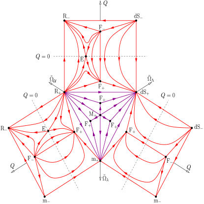
FIG. 3.: Sector corresponding to the dynamics described in subsections III A and III B of the state space for the FLRW models with $\gamma\in(0,\textstyle{1\over 3})$ . It shows that the Einstein universe appears even for $\gamma\leq\textstyle{1\over 3}\,,$ in contrast to what happens in GR and also when ${\cal U}=0\,.$

Coming back to the description of the state space diagrams, the sectors of subsections III B and III C are represented by three rectangular areas, crossed by the dashed lines $Q=0$ and $Z=0$ respectively, enclosing triangular areas corresponding to the sector of subsection III A. The central area, crossed by the line $W=0$, describes the dynamics of the sector in subsection III D. The shadowed region does not belong to the state space, it appears as a result of the two-dimensional representation we have used. The dashed lines $Q=Z=W=0$, where the Hubble function vanishes, separate regions of expanding models from regions with contracting models. Using this structure for the state space, the trajectories follow directly from the information given in the previous subsections.

The attractors of the evolution are $\mbox{dS}_{+}$, $\mbox{R}_{-}$ and $\mbox{m}_{-}$. More specifically, $\mbox{dS}_{+}$ is an attractor for any value of $\gamma$, whereas $\mbox{R}_{-}$ is an attractor only for $\gamma\leq 2/3$ and $\mbox{m}_{-}$ for $\gamma\geq 2/3$. In fact, $\mbox{R}_{-}$ and $\mbox{m}_{-}$ exchange their role as an attractor at the bifurcation $\gamma=2/3$. Moreover, while $\mbox{dS}_{+}$ is an attractor for models that at some time will become ever expanding, $\mbox{R}_{-}$ and $\mbox{m}_{-}$ are attractors for (re)collapsing models. An interesting feature of the state space is that the volume of the region with models evolving towards $\mbox{dS}_{+}$ decreases as $\gamma$ increases, which means that the region of models collapsing in the future increases. The fact of having models that recollapse is directly connected with the appearance of static models, namely E and S, which are saddle points. In this sense, it is important to remark that the presence of ${\cal U}$ makes the Einstein models to appear for any value of $\gamma$ (see Fig. 3), and the fact that it can be negative leads to the appearance of static models with non-positive spatial curvature, i.e. S. Furthermore, E and S are not isolated critical points but bidimensional surfaces in the state space. The location of these surfaces depending on the value of $\gamma$ has been represented in Fig. 4.

FIG. 4.: Surfaces of saddle critical points corresponding to static FLRW models ($H=0$). The diagram on the left is the submanifold $Z=0$ of the sector ${}^{3}R\leq 0$ and ${\cal U}\leq 0$ and the critical points represented correspond to S. The diagrams on the center (right) show the location of the points E in the submanifolds $W=0$ ($Q=0$) of the sector ${}^{3}R\geq 0$ and ${\cal U}\leq 0$ (${}^{3}R\geq 0$ and ${\cal U}\geq 0$). Note that $Q=0$, $Z=0$ and $W=0$ are not invariant submanifolds and therefore they do not contain any trajectories.

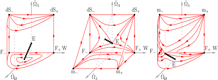
FIG. 5.: Three-dimensional diagrams for the sector ${}^{3}R\geq 0$ and ${\cal U}\leq 0$ of the state space of the FLRW models for $\gamma\in(\textstyle{2\over 3},\textstyle{4\over 3})$. Starting from the left, they correspond to the invariant submanifolds $\hat{\Omega}_{\lambda}=0$, $\hat{\Omega}_{\cal U}=0$ and $\hat{\Omega}_{\Lambda}=0\,.$ The curved part of the boundary of the first and third state space diagrams correspond to the invariant submanifold $W^{2}-\hat{\Omega}_{\cal U}=1$. In these diagrams we also have closed trajectories describing oscillating universes.

The way of compactifying the state space for the sectors of subsections III A and III B is the same as the one used in Paper I for the sectors ${}^{3}R\leq 0$ and ${}^{3}R\geq 0$ respectively. The compactification of the sector in subsection III C is very similar to that of subsection III B, the only difference is that the negative term in the Friedmann equation is due to ${\cal U}$ instead of ${}^{3}R$. In fact, as we can see in Figs. 1 and 2, the structure is almost the same. For the sector corresponding to subsection III D the situation is different due to the appearance of two non-positive contributions to the Friedmann equation. The compactification of the state space in this case leads to a new type of diagrams (see Fig. 5). To understand the dynamics we have to take into account that now we have the following invariant submanifold

$$W^{2}-\hat{\Omega}_{\cal U}=1\,.$$ (34)

It divides the allowed rectangle $[-1,1]\times[-1,0]$ in the plane $(W,\hat{\Omega}_{\cal U})$ into two regions with opposite sign of the spatial scalar curvature. From the definition of $P$ we find

$\displaystyle W^{2}-\hat{\Omega}_{\cal U}-1=\frac{{}^{3}R}{6P^{2}}\,.$

Since ${}^{3}R\geq 0$, this means that only the interior region defined by (34) is allowed (see Fig. 5). The special structure of this sector of the state space leads to a new exceptional feature consisting in the appearance of closed trajectories (see Figs. 1 and 5). They correspond to cosmological models that after a certain period of time come back to the same situation as in the beginning of that period, and for this reason we will call them oscillating universes. As we can see in Fig. 1 the trajectories followed by these models have a minimum and a maximum value of $W$ which, from Eq. (29), satisfy the following relation

$\displaystyle(1-W^{2})\left\{\frac{3\gamma}{2}(\hat{\Omega}_{\rho}+2\hat{\Omega}_{\lambda})-1\right\}=-\hat{\Omega}_{\cal U}\,.$

This equation has solutions only for $\gamma\geq\textstyle{1\over 3}$, just for the values of $\gamma$ that oscillating universes appear in the state space. Moreover, there is also a minimum and a maximum of $\hat{\Omega}_{\cal U}$ that corresponds to $W=0$. In fact, all the quantities describing these models are periodic and therefore have a minimum and a maximum value, in particular the scale factor $a(t)$ and the energy density $\rho$. Hence, these models do not have any spacelike singularity. In Fig. 6 we have represented the evolution of a particular class of oscillating universes. Apart from the features just described it is worth noting that while the transition from the expanding to the contracting stage is smooth, the converse is abrupt and mimics a non-singular bang or bounce. The avoidance of the singularity is due to the negative contribution of the dark-energy density term ${\cal U}$, which goes like $a^{-4}$, to the universe expansion in the Friedmann equation (9). In the contracting stage this term grows and counterbalances the positive contributions in the Friedmann equation, stopping the expansion. This can only happen for $\textstyle{1\over 3}<\gamma<\textstyle{2\over 3}$ when the effect of the $\rho^{2}$ term, which goes like $a^{-6\gamma}$, is dominant, and for $\textstyle{2\over 3}<\gamma<\textstyle{4\over 3}$ (see Fig. 5) when the effect of the $\rho$ term, which goes like $a^{-3\gamma}$, dominates. After the bounce, the universe expands until the spatial curvature ${}^{3}R$, which goes like $a^{-2}$, stops the expansion to enter again a contraction era.

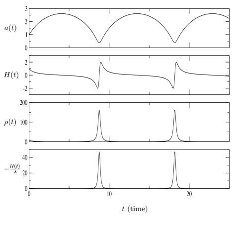
FIG. 6.: Evolution of an oscillating FLRW universe with $k=1$, $\gamma=1$ (dust), $\Lambda=0$, and negligible contribution from the term quadratic in the energy density. We have taken $\kappa=1$ and initial data: $a(0)=H(0)=1$, $\rho(0)=9$ and ${\cal U}(0)=-\lambda$.

IV Dynamics of the Bianchi type I models

In what follows we will complete the dynamical study of Bianchi type I models made in Paper I. Other works on these models in brane-world scenarios can be found in [15, 16, 17]. Exact solutions on the brane have been considered in [18], and a five-dimensional solution for the vacuum case has been presented in [19].

As we have discussed above, the non-zero contributions from the five-dimensional Weyl tensor are ${\cal U}$ and ${\cal P}_{ab}$ but since the second one has no evolution equation we will take ${\cal P}_{ab}=0$. Then, we have to consider two differentiated cases according to the sign of ${\cal U}$: (A) ${\cal U}\geq 0$; (B) ${\cal U}\leq 0$.

A Case ${\cal U}\geq 0$

The treatment of this case is very similar to that made in subsection III A. We will use the dimensionless variables $\mbox{\boldmath$\Omega$}=(\Omega_{\rho},\Omega_{\Lambda},\Omega_{\sigma},\Omega_{\lambda},\Omega_{\cal U})$ [See Eqs.(14) and (15)], where we have defined a normalized variable for the shear contribution

$$\Omega_{\sigma}\equiv\frac{\sigma^{2}}{3H^{2}}\,.$$ (35)

The Friedmann equation (9) then becomes

$\displaystyle\Omega_{\rho}+\Omega_{\Lambda}+\Omega_{\sigma}+\Omega_{\lambda}+\Omega_{\cal U}=1\,,$

and again the state space is compact. Using the time derivative ${}^{\prime}\equiv|H|^{-1}d/dt$ the system of dynamical equations is

$$\Omega^{\prime}_{\rho} = \epsilon[2(1+q)-3\gamma]\Omega_{\rho}\,,$$ (36)

$$\Omega^{\prime}_{\Lambda} = 2\epsilon(1+q)\Omega_{\Lambda}\,,$$ (37)

$$\Omega^{\prime}_{\sigma} = 2\epsilon(q-2)\Omega_{\sigma}\,,$$ (38)

$$\Omega^{\prime}_{\lambda} = 2\epsilon(1+q-3\gamma)\Omega_{\lambda}\,,$$ (39)

$$\Omega^{\prime}_{\cal U} = 2\epsilon(q-1)\Omega_{\cal U}\,,$$ (40)

where $q$ has the following expression

$\displaystyle q=\frac{3\gamma-2}{2}\Omega_{\rho}+(3\gamma-1)\Omega_{\lambda}+2\Omega_{\sigma}-\Omega_{\Lambda}+\Omega_{\cal U}\,.$

The critical points of the dynamical system (36)-(40), their coordinates in the state space and their eigenvalues are given in the next table

Model	Coordinates	Eigenvalues
$\mbox{F}_{\epsilon}$	$(1,0,0,0,0)$	$\epsilon(3\gamma-2,3\gamma,3(\gamma-2),-3\gamma,3\gamma-4)$
$\mbox{dS}_{\epsilon}$	$(0,1,0,0,0)$	$-\epsilon(3\gamma,2,6,6\gamma,4)$
$\mbox{K}_{\epsilon}$	$(0,0,1,0,0)$	$\epsilon(-3(\gamma-2),6,4,-6(\gamma-1),2)$
$\mbox{m}_{\epsilon}$	$(0,0,0,1,0)$	$2\epsilon(\textstyle{3\gamma\over 2},3\gamma,3(\gamma-1),3\gamma-1,3\gamma-2)$
$\mbox{R}_{\epsilon}$	$(0,0,0,0,1)$	$\epsilon(-(3\gamma-4),4,-2,-2(3\gamma-2),2)$

The critical point K corresponds to the vacuum Kasner models of GR, whose line element is given by (7) with

$$A_{\alpha}=t^{2p_{\alpha}}~{}~{}\mbox{and}~{}~{}\sum_{\alpha=1}^{3}p_{\alpha}=\sum_{\alpha=1}^{3}p^{2}_{\alpha}=1\,.$$ (41)

With respect to the analysis of Bianchi type I models done in Paper I, the only new critical points are the radiation models $\mbox{R}_{\pm}\,.$

B Case ${\cal U}\leq 0$

The procedure we will follow in this case is the same as in subsection III C. We will consider the following set of variables $\mbox{\boldmath$\bar{\Omega}$}=(Z,\bar{\Omega}_{\rho},\bar{\Omega}_{\Lambda},\bar{\Omega}_{\sigma},\bar{\Omega}_{\lambda})$ [See Eq. (23)], where $\bar{\Omega}_{\sigma}$ is the analogous of $\Omega_{\sigma}$ (35) but normalized with respect to $N$ (23). With this variables the Friedmann equation (9) reads

$$\bar{\Omega}_{\rho}+\bar{\Omega}_{\Lambda}+\bar{\Omega}_{\sigma}+\bar{\Omega}_{\lambda}=1\,,$$ (42)

and the deceleration parameter $q$ is given by

$\displaystyle(q-1)Z^{2}=\textstyle{{3\gamma}\over 2}(\bar{\Omega}_{\rho}+2\bar{\Omega}_{\lambda})+3\bar{\Omega}_{\sigma}-2\,.$

With respect to the time derivative ${}^{\prime}\equiv N^{-1}d/dt$, the dynamical system for $\bar{\Omega}$ is

$$Z^{\prime} = -(q-1)Z^{2}(1-Z^{2})\,,$$ (43)

$$\bar{\Omega}^{\prime}_{\rho} = -[(3\gamma-4)-2(q-1)Z^{2}]Z\bar{\Omega}_{\rho}\,,$$ (44)

$$\bar{\Omega}^{\prime}_{\Lambda} = 2[2+(q-1)Z^{2}]Z\bar{\Omega}_{\Lambda}\,,$$ (45)

$$\bar{\Omega}^{\prime}_{\sigma} = -2[1-(q-1)Z^{2}]Z\bar{\Omega}_{\sigma}\,,$$ (46)

$$\bar{\Omega}^{\prime}_{\lambda} = -2[(3\gamma-2)-(q-1)Z^{2}]Z\bar{\Omega}_{\lambda}\,.$$ (47)

The critical points of the dynamical system (43)-(47), their coordinates in the state space and their eigenvalues are given in the next table [13]

Model	Coordinates	Eigenvalues
$\mbox{F}_{\epsilon}$	$(\epsilon,1,0,0,0)$	$\epsilon(3\gamma-4,3\gamma,3\gamma,3(\gamma-2),-3\gamma)$
$\mbox{dS}_{\epsilon}$	$(\epsilon,0,1,0,0)$	$-\epsilon(4,3\gamma,0,6,6\gamma)$
$\mbox{K}_{\epsilon}$	$(\epsilon,0,0,1,0)$	$\epsilon(2,-3(\gamma-2),6,6,-6(\gamma-1))$
$\mbox{m}_{\epsilon}$	$(\epsilon,0,0,0,1)$	$2\epsilon(3\gamma-2,\textstyle{{3\gamma}\over 2},3\gamma,3(\gamma-1),3\gamma)$
nE	$(0,\bar{\Omega}^{\ast}_{\rho},\bar{\Omega}^{\ast}_{\Lambda},\bar{\Omega}^{\ast}_{\sigma},\bar{\Omega}^{\ast}_{\lambda})$	$(0,\sqrt{\zeta},0,0,-\sqrt{\zeta})$

We have a new set of saddle critical points, designated by nE, whose coordinates in the state space $\bar{\Omega}^{\ast}$ satisfy (42) and

$\displaystyle\textstyle{{3\gamma}\over 2}(\bar{\Omega}^{\ast}_{\rho}+2\bar{\Omega}^{\ast}_{\lambda})+3\bar{\Omega}^{\ast}_{\sigma}-2=0\,.$

The quantity $\zeta$ is given by

$\displaystyle\zeta=\frac{3\gamma}{2}\left[(3\gamma-4)\bar{\Omega}^{\ast}_{\rho}+4(3\gamma-2)\bar{\Omega}^{\ast}_{\lambda}\right]+6\bar{\Omega}^{\ast}_{\sigma}\,,$

and in the FLRW limit, $\sigma=0\,,$ it corresponds to the quantity $\psi$ in (26) for $k=0$. The nE models are non-expanding ($H=0$) Bianchi models which in the FLRW limit become static, in fact, in this limit, they coincide with the critical points S with ${}^{3}R=0$. A noteworthy difference is that the models S only appear for $\gamma\geq 2/3$ whereas the models nE appear for all values of $\gamma$. Moreover, $\rho\,,$ $\sigma$ and ${\cal U}$ are constants, $(\rho^{\ast},\sigma^{\ast},{\cal U}^{\ast})\,,$ which, in order to have a positive energy density must satisfy a condition analogous to (27)

$\displaystyle-{\cal U}^{\ast}\geq\frac{\lambda\kappa^{2}}{6}\left(\Lambda+{\sigma^{\ast}}^{2}\right)\,.$

In fact, integrating the effective Einstein equations (2), we can find the metric functions $A_{\alpha}(t)$ in (7) corresponding to the critical points nE,

$\displaystyle A_{\alpha}(t)=\mbox{e}^{q_{\alpha}t}\,,$

where $q_{\alpha}$ ($\alpha=1-3$) are constants (proportional to the components of the shear tensor) such that

$\displaystyle\sum_{\alpha=1}^{3}q_{\alpha}=0~{}~{}\mbox{and}~{}~{}\sum_{\alpha=1}^{3}q^{2}_{\alpha}=2{\sigma^{\ast}}^{2}\,.$

Note that despite the scalar factor remains constant ($\prod_{\alpha=1}^{3}A_{\alpha}(t)=1$) the matter can expand or contract along the shear principal axes. In fact, when only one $q_{\alpha}$ is negative the system evolves towards a pancake singularity, whereas when two of them are negative it evolves towards a cigar singularity (for details on this type of singularities see, e.g., [20]).

C Qualitative analysis

To analyze the dynamics we have to consider first the character of the critical points, which can be deduced from the information given in the previous subsections and can be summarized in the following table

Model	Dynamical character
	$0<\gamma<1$	$\gamma=1$	$\gamma>1$
$\mbox{F}_{\pm}$	saddle	saddle	saddle
$\mbox{dS}_{+}$	attractor	attractor	attractor
$\mbox{dS}_{-}$	repeller	repeller	repeller
$\mbox{K}_{+}$	repeller	repeller	saddle
$\mbox{K}_{-}$	attractor	attractor	saddle
$\mbox{m}_{+}$	saddle	repeller	repeller
$\mbox{m}_{-}$	saddle	attractor	attractor
$\mbox{R}_{\pm}$	saddle	saddle	saddle
nE	saddle	saddle	saddle

The character of the critical points $\mbox{F}_{\pm}$, $\mbox{dS}_{\pm}$, $\mbox{K}_{\pm}$, and $\mbox{m}_{\pm}$ is the same as in the case ${\cal U}=0$ studied in Paper I. The new dynamical features are due to the appearance of the critical points $\mbox{R}_{\pm}$ and nE. Moreover, we also find two new bifurcations at $\gamma=\textstyle{2\over 3}$ and $\gamma=\textstyle{4\over 3}$, besides the bifurcations at $\gamma=0,1,2$ already found in Paper I for the case ${\cal U}=0$.

The state space for Bianchi type I models is also four-dimensional and is divided into two sectors according to the sign of ${\cal U}$. We have used the same type of bidimensional representation in which only the trajectories for the two-dimensional invariant submanifolds are drawn. In Fig. 7 we show the state space for $\gamma\in(1,\textstyle{4\over 3})$, which includes physically well-motivated situations from dust to radiation universes. The sector ${\cal U}\leq 0$ described in subsection IV B is represented by three rectangular regions which enclose a triangle where the dynamics of the sector ${\cal U}\geq 0$ (subsection IV A) is depicted. The dashed lines $Z=0$ divided regions of expanding models from regions of contracting models, and these are the places where the non-expanding models nE appear. In fact, these saddle points are not isolated points but two-dimensional surfaces. The location of the surfaces of points nE for different values of $\gamma$ has been drawn in Fig. 8.

For the sector ${\cal U}\geq 0$ the general attractor is de Sitter, as it happens when ${\cal U}=0$. The situation changes for the sector ${\cal U}\leq 0$, where the possible final states of the evolution are $\mbox{dS}_{+}$, $\mbox{K}_{-}$ and $\mbox{m}_{-}$. Like in some sectors of state space of the FLRW models, the sector ${\cal U}\leq 0$ of Bianchi models is divided into two regions, the region of models that will approach $\mbox{dS}_{+}$ and then will become ever expanding, and the region of models that will (re)collapse. Obviously the models approaching $\mbox{dS}_{+}$ in the future isotropize, although there is an intermediate stage in which the relative contribution of shear grows and reaches a maximum. In the sector ${\cal U}\geq 0$ this maximum is reached when the following condition holds (see [17])

$\displaystyle\Omega_{\sigma}=1-\textstyle{2\over 3}\Omega_{\cal U}-\textstyle{\gamma\over 2}(\Omega_{\rho}+2\Omega_{\lambda})\,,$

and in the sector ${\cal U}\leq 0$ the condition is

$\displaystyle\bar{\Omega}_{\sigma}=1-\textstyle{\gamma\over 2}(\bar{\Omega}_{\rho}+2\bar{\Omega}_{\lambda})\,.$

On the other hand, the attractor for collapsing models (${\cal U}\leq 0$) is in general $\mbox{K}_{-}$ ($\mbox{m}_{-}$ for the submanifold $\sigma=0$) for $0<\gamma<1$ and $\mbox{m}_{-}$ ($\mbox{K}_{-}$ for the submanifolds $\bar{\Omega}_{\lambda}=0$) for $\gamma>1$. For dust ($\gamma=1$) we have a bifurcacion in which the attractors are anisotropic models whose line element is the same as the one of Kasner models [see Eqs.(7),(41)] but the constant $p_{\alpha}$ now only satisfy

$\displaystyle\sum_{\alpha=1}^{3}p_{\alpha}=1\,.$

From this discussion we deduce that there are sets of trajectories in the state space that either do not isotropize in the future or isotropize but the final state is not de Sitter ($\mbox{dS}_{+}$). Hence, the cosmic no-hair theorem is not satisfied in the ${\cal U}\leq 0$ sector. This fact has been anticipated in the analysis made in [16], although in their non-compact representation of the state space the final state for collapsing models was not shown.

Finally, with regard to the structure of the initial singularity, in Paper I we showed that for ${\cal U}=0$ and $\gamma\geq 1$ the initial singularity is isotropic, in contrast to what happens in GR. Now, this is also true for the sector ${\cal U}>0$. In the sector ${\cal U}<0$ the singularity is also isotropic except for the submanifold $\bar{\Omega}_{\lambda}=0$.

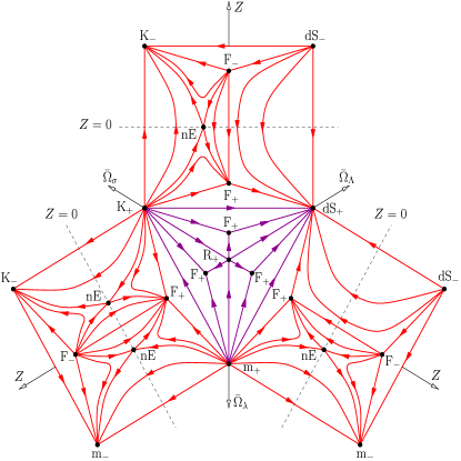
FIG. 7.: Complete state space for Bianchi type I models with $\gamma\in(1,\textstyle{4\over 3})\,.$

FIG. 8.: Representation of surfaces of saddle critical points corresponding to the non-expanding models nE in the $Z=0$ submanifold of the state space of Bianchi type I models.

V Remarks and conclusions

In this paper we have completed the dynamical systems analysis on the evolution of cosmological models in brane-world type scenarios started in Paper I, where the effects of the five-dimensional (bulk) Weyl tensor were not considered. By including this quantity in the analysis we have constructed the most complete state space for non-tilted perfect-fluid FLRW cosmological models. In the case of Bianchi type I models the state space we have presented is also complete except for the fact that we have disregarded the components of the five-dimensional Weyl tensor for which the theory does not provide evolution equations, namely ${\cal P}_{ab}$. This means that we cannot make predictions on how the term ${\cal P}_{ab}$ affects the dynamics. Perhaps future studies on string/M-theory could shed light on this question.

From the dynamical study carried out we have found new interesting features not present in GR nor in brane-world scenarios with ${\cal U}=0$. In particular, we have discovered new critical points: $\mbox{R}_{\pm}$, S and nE. The Einstein universe E and the non-expanding anisotropic models nE appear for any value of $\gamma$, which is directly connected to the fact that we have now (re)collapsing models both for FLRW and Bianchi type I models for any $\gamma$. It is also worth noting that now we have static critical points for any sign of the spatial curvature ${}^{3}R$. We have also seen that de Sitter ($\mbox{dS}_{+}$) is always an attractor but not the only one. For FLRW models, $\mbox{R}_{-}$ and $\mbox{m}_{-}$ are also attractors for $\gamma\leq\textstyle{2\over 3}$ and $\gamma\geq\textstyle{2\over 3}$ respectively, and for Bianchi type I models, $\mbox{K}_{-}$ and $\mbox{m}_{-}$ are attractors for $\gamma\leq 1$ and $\gamma\geq 1$ respectively.

A relevant interesting feature is the appearance of oscillating universes in the ${}^{3}R\geq 0$ and ${\cal U}\leq 0$ sector of the state space of the FLRW models. In these universes the physical variables oscillate periodically between a minimum and a maximum value without reaching any spacelike singularity. With regard to the evolution of the anisotropy in Bianchi type I models we have found that for ${\cal U}\geq 0$ they always isotropize whereas for ${\cal U}\leq 0$ they can both isotropize or collapse. This violation of the cosmic no-hair theorem has also been pointed out in [16]. The use in the present paper of dynamical variables that compactify the state space allows us to see clearly which are the possible final states of the collapse ($\mbox{K}_{-}$ or $\mbox{m}_{-}$) and how the state space is divided into two regions according to whether the models isotropize or collapse. On the other hand, we have seen that the initial singularity is isotropic for $\gamma\geq 1$, as it also happens in the particular case ${\cal U}=0$.

Finally, the analysis we have carried out in this paper provides information on the question of the stability of the so-called Randall-Sundrum fine-tuning condition, which consists in the vanishing of the four-dimensional cosmological constant ($\Lambda=0$). More specifically, in brane-world scenarios the four-dimensional cosmological constant is given by

$\displaystyle\Lambda=\frac{|\Lambda_{(5)}|}{2}\;\left[\left(\frac{\lambda}{\lambda_{c}}\right)^{2}-1\right]\,,~{}~{}~{}\lambda^{2}_{c}\equiv 6\frac{|\Lambda_{(5)}|}{\kappa^{4}_{(5)}}\,,$

where $\lambda_{c}$ is a critical tension. Then the fine tuning consists in adjusting the brane tension $\lambda$ so that $\lambda=\lambda_{c}$. From our perspective, we can deal with this question by asking whether or not the invariant submanifold $\Omega_{\Lambda}=0$ (and also the equivalent ones $\tilde{\Omega}_{\Lambda}=\bar{\Omega}_{\Lambda}=\hat{\Omega}_{\Lambda}=0$), where the fine-tuning condition holds, is dynamically stable. In other words, what happens when initial conditions are prescribed near this invariant submanifold of the state space. It can be seen that for the regions of recollapsing models the evolution will bring them back to $\Omega_{\Lambda}=0$, although if we start with $H>0$ the models will initially separate from that submanifold. For the other regions, the evolution will move the models away from $\Omega_{\Lambda}=0$ in such a way that they will approach de Sitter, which is precisely the opposite situation to $\Lambda=0$ (see also [21] for an alternative discussion). Then, we can conclude that the fine-tuning condition is not dynamically stable in the sense that there are non-zero measure regions of initial data near the fine-tuning $\Lambda=0$ evolving towards a situation in which that condition does not longer hold.

Acknowledgements: The authors wish to thank their colleagues in the Relativity and Cosmology Group for fruitful discussions. This work has been supported by the European Commission (contracts HPMF-CT-1999-00149 and HPMF-CT-1999-00158).

REFERENCES

- [1] L. Randall and R. Sundrum, Phys. Rev. Lett 83, 4690 (1999).
- [2] P. Hoava and E. Witten, Nucl. Phys. B460, 506 (1996); P. Hoava and E. Witten, Nucl. Phys. B475, 94 (1996).
- [3] K. Benakli, Int. J. Mod. Phys. D 8, 153 (1999); A. Lukas, B. A. Ovrut, K. S. Stelle, and D. Waldram, Phys. Rev. D 59, 086001 (1999); H. S. Reall, Phys. Rev. D 59, 103506 (1999); A. Lukas, B. A. Ovrut, and D. Waldram, Phys. Rev. D 60, 086001 (1999); A. Lukas, B. A. Ovrut, and D. Waldram, Phys. Rev. D 61, 023506 (1999); A. P. Billyard, A. A. Coley, J. E. Lidsey, and U. S. Nilsson, Phys. Rev. D 61, 043504 (2000).
- [4] P. Bintruy, C. Deffayet, and D. Langlois, Nucl. Phys. B565, 269 (2000).
- [5] P. Bintruy, C. Deffayet, U. Ellwanger, and D. Langlois, Phys. Lett. B 477, 285 (2000).
- [6] T. Shiromizu, K. Maeda, and M. Sasaki, Phys. Rev. D 62, 024012 (2000).
- [7] M. Sasaki, T. Shiromizu, and K. Maeda, Phys. Rev. D 62, 024008 (2000).
- [8] A. Campos and C. F. Sopuerta, Phys. Rev. D 63, 104012 (2001).
- [9] R. Maartens, Phys. Rev. D 62, 084023 (2000).
- [10] S. W. Hawking and G. F. R. Ellis, The large scale structure of space-time (Cambridge University Press, Cambridge, 1973).
- [11] J. Wainwright and G. F. R. Ellis, Dynamical systems in cosmology (Cambridge University Press, Cambridge, 1997); A. A. Coley, in Proceedings of the Spanish Relativity Meeting. ERE-99, edited by J. Ibáñez (Euskal Herriko Unibertsitatea, Bilbo, 2000).
- [12] D. K. Arrowsmith and C. M. Place, An introduction to dynamical systems (Cambridge University Press, Cambridge, 1990); D. W. Jordan and P. Smith, Nonlinear ordinary differential equations. An introduction to dynamical systems (Oxford University Press, Oxford, 1999).
- [13] The presence of a zero eigenvalue is (excepting for bifurcations and the sets of critical points E, S and nE) a consequence of having a dynamical system with a constraint: The Friedmann equation. If we had used it to eliminate one variable and reduce the dimension of the state space, we would not find any vanishing eigenvalue. In conclusion, this fact does not affect to the hyperbolic character of the critical points.
- [14] . . Flanagan, S.-H. H. Tye, and I. Wasserman, Phys. Rev. D 62, 044039 (2000).
- [15] R. Maartens, V. Sahni and T. D. Saini, Phys. Rev. D 63, 063509 (2001).
- [16] M. G. Santos, F. Vernizzi, and P. G. Ferreira, hep-ph/0103112.
- [17] A. V. Toporensky, gr-qc/0103093.
- [18] C.-M. Chen, T. Harko, and M. K. Mak, hep-th/0103240.
- [19] A. V. Frolov, gr-qc/0102064
- [20] H. Stephani, General Relativity (Cambridge University Press, Cambridge, 1990).
- [21] T. Boehm, R. Durrer, and C. van de Bruck, hep-th/0102144.