hep-th/0105077 McGill/01-03

UTPT-01-07

NSF-ITP-01-21

DCTP–01/35

The enhançon mechanism removes a family of time–like singularities from certain supergravity spacetimes by forming a shell of branes on which the exterior geometry terminates. The problematic interior geometry is replaced by a new spacetime, which in the prototype extremal case is simply flat. We show that this excision process, made inevitable by stringy phenomena such as enhanced gauge symmetry and the vanishing of certain D–branes’ tension at the shell, is also consistent at the purely gravitational level. The source introduced at the excision surface between the interior and exterior geometries behaves exactly as a shell of wrapped D6–branes, and in particular, the tension vanishes at precisely the enhançon radius. These observations can be generalised, and we present the case for non–extremal generalisations of the geometry, showing that the procedure allows for the possibility that the interior geometry contains an horizon. Further knowledge of the dynamics of the enhançon shell itself is needed to determine the precise position of the horizon, and to uncover a complete physical interpretation of the solutions.

1 Introduction

In ref. [1], the study of the supergravity fields produced by a family of brane configurations revealed a new mechanism by which string theory removes a class of time–like naked singularities. The singularities, of “repulson” type, arise at the locus of points where parts of the ten dimensional geometry shrink to zero size. The supergravity geometries preserve eight supercharges. In the prototype example of ref. [1] it is a K3 manifold (on which the branes are wrapped) which shrinks to zero size, but the presence of a K3 is not essential for the phenomenon.

In short, the naïve supergravity solution is modified by the fact that the constituent branes which source the fields smear out from being point–like (in their transverse space) to being a sphere. This sphere is called the “enhançon”. Pure supergravity is unable to model this phenomenon, because it is controlled by physics which arises before the shrinking parts of the geometry get to zero size. Instead, when they get to volumes set by a characteristic length $2\pi\sqrt{\alpha^{\prime}}$, new massless modes appear in the string theory. In ref. [1], the shrinking volume of K3 gets to $V_{*}=(2\pi\sqrt{\alpha^{\prime}})^{4}$, and there is an enhanced gauge symmetry $U(1)\to SU(2)$. The unwrapped parts of the D–branes are monopoles of the $U(1)$ and correspondingly become massless and expand at this place, forming the enhançon.

The supergravity geometry interior to the enhançon, containing the repulson singularity, is obviously incorrect, as it exhibits a number of unphysical properties uncovered in, for example, refs. [1, 2, 3, 4]. In fact, since it has a naked singularity, the repulson is not only unphysical, it is part of a family of incorrect geometries with the correct asymptotic charges, since no–hair theorems (which are usually relied upon, at least implicitly, to interpret supergravity physics) apply only if a singularity in the proposed geometry is hidden behind an horizon. The proposal [1] was therefore that the repulson be excised and replaced with a more appropriate geometry. In the cases studied in ref. [1], the geometry in the interior is simply flat space, since there are no brane sources in the interior, as they have all expanded out to form the enhançon.

In section 2 of this paper, we will show that this excision procedure is consistent —and in fact is an extremely natural process— in supergravity. By analysing the standard junction conditions, we show in the next section that the enhançon radius is a special place even from the simple point of view of the stress–energy of the shell, and that this stress–energy corresponds precisely to that of a shell of wrapped D6–branes. We also show that the shell provides sources for the dilaton and R–R fields which again match precisely to those of wrapped D6–branes.

In section 3 we generalise this situation slightly by adding D2–branes, to set the stage for section 4, where we study two families of non–extremal generalisations of the enhançon geometry. The first family corresponds to a system combining wrapped D6–branes and a larger number of additional D2–branes. These non–extremal solutions all contain an event horizon, which may or may not appear outside of the enhançon radius. In the case where an event horizon appears below the enhançon radius, the excision procedure gives us a range of choices for the interior solution. It does not appear that this ambiguity can be resolved within the supergravity framework alone.

The second family, which is characterised by a repulson–like singularity (before any excision) is an extension of those derived in ref. [1]. This solution seems to describe a non–extremal configuration with arbitrary numbers of D2– and D6–branes. However, this solution does not reduce to the previous one when the number of D2–branes exceeds the number of D6–branes, nor does it reduce to a standard D6–brane solution when the volume of the $K3$ is large. Furthermore, this solution also has the peculiar feature that it never has an event horizon outside of the enhançon radius. Hence its physical interpretation remains unclear. Section 5 presents conclusions and discussion of future directions.

Although perhaps in retrospect it could not have been much different, we do find it remarkable that while supergravity cannot produce the stringy phenomena which make the enhançon mechanism necessary, it does display some awareness of the behaviour of the branes that source this geometry; the source terms on the shell correspond to precisely those in the worldvolume action.

2 The Extremal Enhançon

The enhançon story is best told by considering the case of wrapping $N$ D$(p+4)$–branes on a K3 manifold of volume $V$. This leaves an unwrapped $(p+1)$–dimensional worldvolume in the non–compact six dimensions. There are $5-p$ non–compact spatial dimensions transverse to the brane. We shall often use polar coordinates in these directions, since everything we do here will retain rotational symmetry. These coordinates are $r,\{\Omega_{4-p}\}$, where the set $\{\Omega_{4-p}\}$ denotes one’s favourite choice of angular coordinates on a unit round $(4-p)$–sphere, $S^{4-p}$.

The supergravity solution necessarily arranges that the volume of K3 decreases from the value $V$ at $r=\infty$ to smaller values as $r$ decreases. We shall denote this running volume as $V(r)$. Type II string theory compactified on K3 has an enhanced gauge symmetry when the K3 volume reaches $V_{*}=(2\pi)^{4}(\alpha^{\prime})^{2}$, in our units. The special radius at which this happens is called the enhançon radius and denoted $r_{\rm e}$. We give its value below.

2.1 The Geometry

To avoid unnecessary notational clutter we focus on the case $p=2$. For the issues that we consider, the extension to other $p$ is trivial, and so we suppress those cases in the discussion, but the reader may wish to keep them in mind for their own purposes. The repulson solution is then

$$ds^{2} = Z_{2}^{-1/2}Z_{6}^{-1/2}\eta_{\mu\nu}dx^{\mu}dx^{\nu}+Z_{2}^{1/2}Z_{6}^{1/2}dx^{i}dx^{i}+V^{1/2}Z_{2}^{1/2}Z_{6}^{-1/2}ds^{2}_{\rm K3}\ ,$$

$$e^{2\Phi} = g_{s}^{2}{Z_{2}}^{1/2}{Z_{6}}^{-3/2}\ ,$$

$$C_{(3)} = ({Z_{2}}g_{s})^{-1}dx^{0}\wedge dx^{1}\wedge dx^{2}\ ,$$

$$C_{(7)} = ({Z_{6}}g_{s})^{-1}dx^{0}\wedge dx^{1}\wedge dx^{2}\wedge V\,\varepsilon_{\rm K3}\ ,$$ (1)

where the above line element corresponds to the string frame metric. Here indices $(\mu,\nu)$ run over the 012–directions along the unwrapped worldvolume, while indices $(i,j)$ run over the 345–directions transverse to the brane. Also, $ds^{2}_{\rm K3}$ is the metric of a K3 surface of unit volume and $\varepsilon_{\rm K3}$ is the corresponding volume form. The harmonic functions are

$$Z_{6} = 1+{r_{6}\over r}\ ,\quad Z_{2}=1-{r_{2}\over r}\ ,$$ (2)

where

$$\quad r_{6}={g_{s}N\alpha^{\prime 1/2}\over 2}\ ,\quad r_{2}={V_{*}\over V}{r_{6}}\ ,$$ (3)

with $N$ being the number of D6–branes. The running K3 volume can be simply read off as

$$V(r)=V{Z_{2}(r)\over Z_{6}(r)}\ .$$ (4)

Using this, a quick computation shows that

$$r_{\rm e}={2V_{*}\over{V}-V_{*}}r_{6}\ .$$ (5)

It is interesting to note that the following is true:

$${\partial\over\partial r}\left(Z_{2}(r)Z_{6}(r)\right)\biggr{|}_{r=r_{\rm e}}=0\ .$$ (6)

This simple result is in fact at the heart of the consistency of the full junction computation we present in the next section, as we shall see.

2.2 Brane Probes

The wrapped D6–branes will expand into a shell of zero tension at $r=r_{\rm e}$. Just to remind the reader, and to set up the notation for the following sections, we reproduce below the probe computation of ref. [1] which supports this conclusion.

The effective worldvolume action of a single wrapped D6–brane, with which we can probe the geometry, is:

$$S=-\int_{{\cal M}_{2}}d^{3}\xi\,e^{-\Phi(r)}(\mu_{6}V(r)-\mu_{2})(-\det{G_{\mu\nu}})^{1/2}+\mu_{6}\int_{{\cal M}_{2}\times\rm K3}\!C_{(7)}-\mu_{2}\int_{{\cal M}_{2}}C_{(3)}\ ,$$ (7)

where ${\cal M}_{2}$ is the unwrapped part of the worldvolume, which lies in six non–compact dimensions, and $G_{\mu\nu}$ is the induced (string frame) metric. Of course, this result includes the subtraction of one fundamental unit of D2–brane tension[5] and R–R charge[6, 7, 8], which results from wrapping the D6–brane on K3. Note the R–R charges $\mu_{p}$ appear in the Dirac–Born–Infeld part of the action since we have included the string coupling $g_{s}$ in the solution for the dilaton. Recall that the basic D–brane tension is given by $\tau_{p}=\mu_{p}/g_{s}$. The fundamental D6- and D2–brane charges are $\mu_{6}=(2\pi)^{-6}\alpha^{\prime-7/2}$ and $\mu_{2}=(2\pi)^{-2}\alpha^{\prime-3/2}$. Note that

$${\mu_{2}\over\mu_{6}}={\mu_{p}\over\mu_{p+4}}=(2\pi)^{4}(\alpha^{\prime})^{2}=V_{*}\ .$$ (8)

It is the fact that this ratio yields $V_{*}$ for all $p$, following from T–duality, which is at the heart of the consistency of the whole mechanism. If it were not true, wrapped D4–branes would become massless at a different value of $r$ from where wrapped D6–branes go massless, and then there would be no W–bosons to carry the enhanced gauge symmetry. This universality also underlies why we can focus on the case $p=2$ without loss of generality.

Choose a static gauge where we align the worldvolume coordinates $\xi^{\mu}$ with the first three spacetime coordinates $(x^{0},x^{1},x^{2})$, and then allow the transverse location of the brane to depend only on time $t\equiv x^{0}$. Next, substitute the exterior solution (1) into the action (7), and expand it, keeping only quadratic order in velocity in $x^{i}$. In this way, one can write the effective Lagrangian density for the problem of moving the probe brane slowly in the background produced by all of the other branes, ${\cal L}=T(r,\theta,\phi)-U(r)$. As this is a supersymmetric problem, $U(r)$ is constant (it is zero in our conventions), while for the kinetic energy we have:

$${T} \equiv {1\over 2}\tau(r)v^{2}={1\over 2g_{s}}(\mu_{6}VZ_{2}-\mu_{2}Z_{6})v^{2}$$ (9)

$$= {\mu_{2}Z_{6}(r)\over 2g_{s}}\left[{V(r)\over V_{*}}-1\right][{\dot{r}}^{2}+r^{2}({\dot{\theta}}^{2}+\sin^{2}\theta{\dot{\phi}}^{2})]\ .$$

Note that the second line shows that the kinetic energy (and hence the effective tension $\tau(r)$ of the probe) vanishes precisely at $r=r_{\rm e}$.

If we were to continue the result into the repulson region $r<r_{\rm e}$, we would find that the tension of the probe becomes negative. Fixing that problem by taking the absolute value of the tension then produces another problem: the cancellation of the potential $U(r)$ will fail, which is inconsistent with the supersymmetry of the situation. Therefore the probe cannot proceed any further inside the geometry than the enhançon radius. We should also point out here that more can be deduced [1, 9, 10] about the geometry by exploiting the fact that the brane is in fact a BPS monopole of the six dimensional Higgsed $SU(2)$. So not only does its mass go to zero at the enhanced gauge symmetry point, but its size diverges, and the probe spreads all over the enhançon locus. The enhançon therefore is a shell of smeared branes of zero tension.

Since there are no point–like sources inside, it is not unreasonable to suggest that the interior of the geometry is in fact flat space (in this large $N$ approximation; there will be subleading corrections), and we shall next examine the consistency of this proposal from the point of view of supergravity.

2.3 The Junction Conditions

The brane probe calculation suggests that the repulson geometry is replaced by flat space inside a shell, which is produced by delocalised branes. We can use the classic gravitational techniques [11, 12] to describe this geometry more explicitly, and calculate the stress–energy and charges of the shell matching the exterior repulson geometry to flat space.

If we join two solutions across some surface, there will be a discontinuity in the extrinsic curvature at the surface. This can be interpreted as a $\delta$–function source of stress–energy located at the surface. In the following section, we will show that the value of this source precisely agrees with the source inferred from the D–brane worldvolume action, confirming the consistency of this description.

Let us compute the relevant quantities, working at arbitrary incision radius $r=r_{\rm i}$. The computation should be performed in Einstein frame, to allow us to interpret the discontinuity in the extrinsic curvature as a stress–energy [11, 12]. One gets the ten dimensional Einstein metric from the string one presented in the previous section by the conformal rescaling

$$ds^{2}_{\rm E}=e^{-\Phi/2}ds^{2}_{\rm S}\ ,$$ (10)

and we shall denote the metric components simply as $G_{AB}$, with no further adornment. When we need to refer to string frame metric components, we shall be very explicit.

We are slicing in a direction perpendicular to the coordinate $r$, and so we can define unit normal vectors:

$$n_{\pm}=\mp{1\over\sqrt{G_{rr}}}\,{\partial\over\partial r}\ ,$$ (11)

where $n_{+}$ ($n_{-}$) is the outward pointing normal for the spacetime region $r>r_{\rm i}$ ($r<r_{\rm i}$). In terms of these, the extrinsic curvature of the junction surface for each region is

$$K^{\pm}_{AB}={1\over 2}\,n_{\pm}^{C}\partial_{C}G_{AB}=\mp{1\over 2\sqrt{G_{rr}}}\,{\partial G_{AB}\over\partial r}\ .$$ (12)

The discontinuity in the extrinsic curvature across the junction is defined as $\gamma_{AB}=K^{+}_{AB}+K^{-}_{AB}$, and with these definitions, the stress–energy tensor supported at the junction is simply

$$S_{AB}={1\over\kappa^{2}}\left(\gamma_{AB}-G_{AB}\,\gamma^{C}{}_{C}\right)\ ,$$ (13)

where $\kappa$ is the gravitational coupling, i.e., $2\kappa^{2}=16\pi G_{N}=(2\pi)^{7}(\alpha^{\prime})^{4}g_{s}^{2}$ is the ten dimensional Newton’s constant in our present conventions.

In our case, we want to match the Einstein metric of the repulson,

$$g_{s}^{1/2}\,ds^{2} = Z_{2}^{-5/8}Z_{6}^{-1/8}\eta_{\mu\nu}dx^{\mu}dx^{\nu}+Z_{2}^{3/8}Z_{6}^{7/8}dx^{i}dx^{i}+V^{1/2}Z_{2}^{3/8}Z_{6}^{-1/8}ds^{2}_{K3}$$ (14)

$$= G_{\mu\nu}dx^{\mu}dx^{\nu}+G_{ij}dx^{i}dx^{j}+G_{ab}dx^{a}dx^{b}\ ,$$

where $Z_{2}$ and $Z_{6}$ are given by (2), to a flat metric. We will start with a matching at some arbitrary radius $r=r_{\rm i}$, and will see that $r=r_{\rm e}$ is a special choice. We explicitly ensure that all fields are continuous through the incision by writing the interior solution in appropriate coordinates and gauge,

$$g_{s}^{1/2}ds^{2} = Z_{2}(r_{\rm i})^{-5/8}Z_{6}(r_{\rm i})^{-1/8}\eta_{\mu\nu}dx^{\mu}dx^{\nu}+Z_{2}(r_{\rm i})^{3/8}Z_{6}(r_{\rm i})^{7/8}dx^{i}dx^{i}$$

$$\qquad\qquad\qquad\qquad\qquad\qquad+V^{1/2}Z_{2}(r_{\rm i})^{3/8}Z_{6}(r_{\rm i})^{-1/8}ds^{2}_{\rm K3}\ ,$$

$$e^{2\Phi} = g_{s}^{2}Z_{2}^{1/2}(r_{\rm i})Z_{6}^{-3/2}(r_{\rm i})\ ,$$

$$C_{(3)} = ({Z_{2}(r_{\rm i})}g_{s})^{-1}dx^{0}\wedge dx^{1}\wedge dx^{2}\ ,$$

$$C_{(7)} = ({Z_{6}}(r_{\rm i})g_{s})^{-1}dx^{0}\wedge dx^{1}\wedge dx^{2}\wedge V\,\varepsilon_{\rm K3}\ .$$ (15)

Some computation gives the following results for the discontinuity tensor:

$$\gamma_{\mu\nu} = \phantom{-}{1\over 16}{1\over\sqrt{G_{rr}}}\left(5{Z_{2}^{\prime}\over Z_{2}}+{Z_{6}^{\prime}\over Z_{6}}\right)G_{\mu\nu}\ ,$$

$$\gamma_{ij} = {-}{1\over 16}{1\over\sqrt{G_{rr}}}\left(3{Z_{2}^{\prime}\over Z_{2}}+7{Z_{6}^{\prime}\over Z_{6}}\right)G_{ij}\ ,$$

$$\gamma_{ab} = {-}{1\over 16}{1\over\sqrt{G_{rr}}}\left(3{Z_{2}^{\prime}\over Z_{2}}-{Z_{6}^{\prime}\over Z_{6}}\right)G_{ab}\ ,$$ (16)

where the metric components are as defined in eqn. (14), a prime denotes $\partial_{r}$ and all quantities are evaluated at the incision surface $r=r_{\rm i}$. Note, however, that $\gamma_{AB}$ is a tensor on the nine dimensional junction surface and so $G_{ij}$ denotes the metric on the angular directions of the transverse space, i.e., there is no $\gamma_{rr}$ component. From the above we can compute the trace

$$\gamma^{C}{}_{C}={-}{1\over 16}{1\over\sqrt{G_{rr}}}\left(3{Z_{2}^{\prime}\over Z_{2}}+7{Z_{6}^{\prime}\over Z_{6}}\right)\ .$$ (17)

Putting this all together gives the following pleasing results for the stress–energy tensor at the discontinuity:

$$S_{\mu\nu} = {1\over 2\kappa^{2}\sqrt{G_{rr}}}\left({Z_{2}^{\prime}\over Z_{2}}+{Z_{6}^{\prime}\over Z_{6}}\right)G_{\mu\nu}\ ,$$

$$S_{ij} = 0\ ,$$

$$S_{ab} = {1\over 2\kappa^{2}\sqrt{G_{rr}}}\left({Z_{6}^{\prime}\over Z_{6}}\right)G_{ab}\ .$$ (18)

Let us pause to admire the result. The last line, referring to the stress along the K3 direction, involves only the harmonic function for the pure D6–brane part. This is appropriate, since there are only D6–branes wrapped there. According to the middle line, there is no stress in the directions transverse to the branes. This is consistent with the fact that the constituent branes are BPS, and so there are no inter–brane forces needed to support the shell in the transverse space.

As a first check of this interpretation, we can expand the results in eqn. (18) for large $r_{\rm i}$. Up to an overall sign, the coefficient of the metric components gives an effective tension in the various directions. The leading contributions are simply:

$$\tau_{\rm mem}(r_{\rm i}) = {1\over 2\kappa^{2}}{r_{6}\over r_{\rm i}^{2}}\left(1-{V_{*}\over V}\right)$$ (19)

$$= {N\over(2\pi)^{6}(\alpha^{\prime})^{7/2}g_{s}}(V-V_{*}){1\over 4\pi r^{2}_{\rm i}V}=N(\tau_{6}V-\tau_{2})\left({1\over 4\pi r^{2}_{\rm i}V}\right)\ ,$$

$$\tau_{\rm K3}(r_{\rm i}) = {1\over 2\kappa^{2}}{r_{6}\over r_{\rm i}^{2}}={N\over(2\pi)^{6}(\alpha^{\prime})^{7/2}g_{s}}\left({1\over 4\pi r^{2}_{\rm i}}\right)=N\tau_{6}\left({1\over 4\pi r^{2}_{\rm i}}\right)\ ,$$ (20)

which is in precise accord with expectations. In the K3 directions, the effective tension matches precisely that of $N$ fundamental D6–branes, with an additional averaging factor ($1/4\pi r^{2}_{\rm i}$) coming from smearing the branes over the shell in the transverse space. In the $x^{0,1,2}$ directions, we have an effective membrane tension which, up to the appropriate smearing factor, again matches that for $N$ D6–branes including the subtraction of $N$ units of D2–brane tension as a result of wrapping on the K3 manifold[5].

We will make the matching of our effective stress tensor (18) to a shell of D–brane sources more precise in the following section. At this point, however, notice that the result for the stress–energy in the unwrapped part of the brane is proportional to $(Z_{2}Z_{6})^{\prime}$. As we have already observed in (6), this vanishes at precisely $r=r_{\rm e}$, and therefore we recover the result[1] that for incision at the enhançon radius, there is a shell of branes of zero tension.

For $r<r_{\rm e}$ we would get a negative tension from the stress–energy tensor, which is problematic even in supergravity. Notice however that nothing in our computation shows that we cannot make an incision at any radius of our choosing for $r\geq r_{\rm e}$, and place a shell of branes of the appropriate tension (as in the calculation of the effective tensions at large $r_{\rm i}$ above). This corresponds physically to the fact that probe branes experience no potential, so they can consistently be placed at any arbitrary position outside the enhançon. The special feature of the enhançon radius in both cases is that it is a limit to where we can place the branes. In section 2.5, we show that the enhançon radius is also special from the point of view of particle scattering.

2.4 Matching fields and branes

We have seen that the effective tensions of the shell agree with those expected for a collection of wrapped D6–branes at large radius, and that the membrane tension vanishes at the same place as the tension of the source branes. In fact, it is easily seen that the stress–energy of the shell is in general precisely the same as the stress–energy of $N$ wrapped D6–branes distributed uniformly on the sphere, as we will now show.

The integrated Einstein equation tells us that shell stress–energy should be given by

$$S_{AB}=\int\sqrt{G_{rr}}\,dr\ \left[-{{2}\over{\sqrt{-G}}}\sum_{\rm shell}{{\delta S_{\rm{brane}}}\over{\delta G^{AB}}}\right]\,,$$ (21)

where the sum means that we should sum over the contributions of all of the constituent branes in the shell. The term in the square brackets is just the standard definition for the stress–energy tensor. As the source coming from the shell of branes is a distribution (in the technical sense), the integral is included to eliminate the radial $\delta$–function. Note that it is important here that the variation is made with respect to the Einstein frame metric.

The metric only appears in the Dirac–Born–Infeld part of the D–brane action as can be seen in eqn. (7). Converting this result to Einstein frame, the action for $N$ wrapped D6–branes is

$$S_{\rm DBI}=-N\int_{{\cal M}_{2}}d^{3}\xi\,e^{-\Phi/4}(\mu_{6}e^{\Phi}V_{\rm E}(r)-\mu_{2})(-\det{G_{\mu\nu}})^{1/2},$$ (22)

where $V_{\rm E}(r)$ is the volume of the K3 in Einstein frame, i.e., $V_{\rm E}(r)=\int_{K3}d^{4}x\sqrt{-G_{ab}}$, and now ${G}_{\mu\nu}$ denotes the pull–back of the Einstein frame metric to the effective membrane worldvolume. We assume that the $N$ D6–branes are distributed uniformly over the $S^{2}$. Recall that we work in static gauge with $\xi^{\mu}=x^{\mu},\mu=0,1,2$. The stress–energy of these source branes can then be written as

$$S_{\mu\nu} = {Ne^{-\Phi/4}\over V_{\rm E}{\rm Vol}(S^{2})}(\mu_{2}-\mu_{6}e^{\Phi}V_{\rm E})G_{\mu\nu}={1\over 2\kappa^{2}\sqrt{G_{rr}}}\left({Z_{2}^{\prime}\over Z_{2}}+{Z_{6}^{\prime}\over Z_{6}}\right)G_{\mu\nu},$$

$$S_{ab} = -{Ne^{3\Phi/4}\over{\rm Vol}(S^{2})}\mu_{6}G_{ab}={1\over 2\kappa^{2}\sqrt{G_{rr}}}{Z_{6}^{\prime}\over Z_{6}}G_{ab}.$$ (23)

Thus, we see that the form agrees with the shell stress–energy given in eqn. (18).

Note that we have been slightly cavalier in doing the stress–energy calculation using the effective membrane action in eqn. (22). The correct microscopic action would actually be that for the seven dimensional worldvolume of the wrapped D6–branes. The term proportional to $\mu_{6}$ implicitly takes this form since $V_{\rm E}$ is defined as a four dimensional integral over the K3 surface. However, the contribution proportional to $\mu_{2}$ actually has its origin in an $\alpha^{\prime}$ correction to the standard DBI action for the D6–branes[5]. That is, implicitly this term involves an integral over the K3 of an curvature–squared term and further this combination of curvatures is not a topological invariant. Therefore naïvely it would appear that $S_{ab}$ should actually have contributions proportional to $\mu_{2}$. In fact, however, this contribution vanishes because K3 is Ricci–flat. The difference between the curvature–squared interaction in the D6–brane action and the Gauss–Bonnet invariant is proportional to $2R_{ab}R^{ab}-R^{2}$. Hence the nontrivial contributions coming from the variation of these terms will be proportional to the Ricci tensor or Ricci scalar, and so vanish when evaluated on K3. Similarly the contributions proportional to $\mu_{2}$ in the effective membrane action (7) originate from the integral over K3 of a curvature–squared term in the Wess–Zumino part of the D6–brane action. In this case, these anomaly induced terms do form a four dimensional topological invariant, the first Pontryagin class[7]. Hence there is no contribution to the stress tensor coming from the variation of these terms either.

Hence these results (23) provide a further verification that matching the repulson solution (1) to a flat space interior (15) at any radius has the interpretation of introducing a shell of wrapped D6–branes as the source. As a additional check, we can also consider the matching of the other fields. The simplest to consider are the R–R fields. Since the exterior geometry contains $N$ units of 7–form flux and $-N$ units of 3–form flux, and the interior has none, the shell clearly carries the same R–R charges as $N$ wrapped D6–branes.

It is interesting and instructive to consider the junction conditions for the dilaton in detail. Since this issue is rarely discussed, we begin with the simple case of a shell of extremal D6–branes living unwrapped in flat ten dimensional spacetime. The dilaton and R–R fields are written in terms of the harmonic function ${H}_{6}$ as

$${{e^{\Phi}}}={g_{s}}{H}_{6}^{-3/4}\,,\quad C_{(7)}=({g_{s}{H}_{6}})^{-1}dx^{0}\wedge dx^{1}\wedge dx^{2}\wedge V\,\varepsilon_{\rm K3}\,,$$ (24)

while the metric is, in Einstein frame,

$$ds^{2}={H}_{6}^{-1/8}\left(-dt^{2}+\sum_{i=1}^{6}dx_{i}^{2}\right)+{H}_{6}^{7/8}(dr^{2}+r^{2}d\Omega_{2}^{2})\ .$$ (25)

In this BPS case, the radial component of the metric is continuous at the shell, but this is not true generally. The only requirement is that the induced metric transverse to $r$ be continuous at the shell.

Since the function ${H}_{6}$ is harmonic, for a shell of D6–branes at radius $r_{\rm i}$, Gauss’s law demands

$${H}_{6}(r)=Z_{6}(r_{\rm i})+\theta(r-r_{\rm i})\left[Z_{6}(r)-Z_{6}(r_{\rm i})\right]\ ,$$ (26)

where $Z_{6}(r)$ is as given in eqn. (2). Hence, differentiating with respect to $r$,

$${H}_{6}^{\prime}(r)=\theta(r-r_{\rm i})Z_{6}^{\prime}(r)$$ (27)

and once again

$${H}^{\prime\prime}_{6}(r)=\theta(r-r_{\rm i})Z^{\prime\prime}_{6}(r)+\delta(r-r_{\rm i})Z^{\prime}_{6}(r)\,.$$ (28)

It is the singular delta function which gives rise to the junction conditions. We therefore need to find all the places in which ${H}^{\prime\prime}_{6}$ appears.

For the bulk dilaton equation of motion we have, given the electric coupling to the R–R potential $C_{(7)}$

$$\nabla^{2}\Phi-{{(-3/2)}\over{2(8)!}}e^{-3\Phi/2}(\partial C)^{2}=-{{2\kappa^{2}}\over{\sqrt{-G}}}{{\delta}\over{\delta\Phi}}\sum_{\rm shell}S_{\rm brane}\,.$$ (29)

For the purpose of discovering junction conditions, our only bulk concern here is the Laplacian of the dilaton; the R–R field strength term has too few derivatives. For the left hand side of the bulk equation we therefore have for the singular term just

$$G^{rr}\Phi^{\prime\prime}\simeq-{{3}\over{4}}G^{rr}{H}_{6}(r)^{-1}{H}^{\prime\prime}_{6}(r)\simeq-{{3}\over{4}}{{1}\over{G_{rr}}}{H}_{6}(r)^{-1}\ \delta(r-r_{\rm i}){H}^{\prime}_{6}(r)\,,$$ (30)

or in covariant language

$$\nabla^{2}\Phi\simeq-{{3}\over{4}}{{H}_{6}(r)}^{-1}\ n^{r}\nabla_{r}{H}_{6}(r)\ {{\delta(r-r_{\rm i})}\over{\sqrt{G_{rr}}}}\simeq n^{r}\nabla_{r}\Phi{{\delta(r-r_{\rm i})}\over{\sqrt{G_{rr}}}}\,.$$ (31)

More generally, we can encode the covariant integrated discontinuity as

$$2\kappa^{2}S_{\Phi}\equiv(n^{r}\nabla_{r}\Phi|_{r=r_{\rm i}+\epsilon}-n^{r}\nabla_{r}\Phi|_{r=r_{\rm i}-\epsilon})={{1}\over{\sqrt{G_{rr}}}}(\Phi^{\prime}|_{r=r_{\rm i}+\epsilon}-\Phi^{\prime}|_{r=r_{\rm i}-\epsilon})\,.$$ (32)

For the brane source term, we begin with the usual DBI brane action, as the Wess–Zumino term couples only to the bulk R–R field. The D6–branes of the shell are distributed evenly over the transverse two–sphere ($\Omega$), so that

$$\begin{array}[]{l}\vspace{5pt}{\displaystyle{-{{2\kappa^{2}}\over{\sqrt{-G}}}{{\delta}\over{\delta\Phi(y)}}\sum_{\rm shell}S_{\rm brane}}}\cr\vspace{5pt}={\displaystyle{2\kappa^{2}\left(\int d^{2}\Omega\,{{N}\over{4\pi}}\right)\left[{{\mu_{6}}\over{g_{s}}}\int d^{7}\xi\left({{3}\over{4}}\right)e^{3\Phi(x)/4}\sqrt{-\det{G_{\mu\nu}}(x)}\right]{{\delta^{10}(y-x(\xi))}\over{{\sqrt{-G}}}}}}\cr={\displaystyle{{{3\kappa^{2}\mu_{6}N}\over{8\pi g_{s}}}\,{{\delta(r-r_{\rm i})}\over{\sqrt{G_{rr}G_{\Omega\Omega}}}}\,e^{3\Phi(r)/4}}}\,.\end{array}$$ (33)

Here it is important that the variation of the dilaton is made while holding the Einstein frame metric fixed. The BPS D6–brane shell therefore gives the source

$$2\kappa^{2}S_{\Phi}={{3\kappa^{2}\mu_{6}N}\over{8\pi g_{s}}}\,{{e^{3\Phi(r)/4}}\over{\sqrt{G_{\Omega\Omega}}}}\,.$$ (34)

We want to show that eqns. (32) and (34) agree. Using $\Phi^{\prime}=-3H_{6}^{\prime}/4H_{6}$, and continuity of $H_{6}$, this will be true if

$$-({H}^{\prime}_{6}(r)|_{r=r_{\rm i}+\epsilon}-{H}^{\prime}_{6}(r)|_{r=r_{\rm i}-\epsilon})={{\kappa^{2}\mu_{6}N}\over{2\pi g_{s}}}\ {{{{H}_{6}(r)\sqrt{G_{rr}}}e^{3\Phi(r)/4}}\over{\sqrt{G_{\Omega\Omega}}}}=2\kappa^{2}{{N\mu_{6}}\over{4\pi r_{\rm i}^{2}}g_{s}}.$$ (35)

Note that the factors of ${H}_{6}$ have cancelled in a non–trivial manner. Thus, this result is consistent with the usual form of the harmonic function; i.e., eqn. (35) is satisfied if $Z_{6}$ takes its usual form,

$$\mu_{6}=(2{\pi})^{-6}{\alpha^{\prime}}^{-7/2}\longrightarrow Z_{6}(r)=1+{{r_{6}}\over{r}}\ ,\qquad r_{6}\equiv{g_{s}N{\alpha^{\prime}}^{1/2}\over 2}\ .$$ (36)

Thus, for a spherical shell of unwrapped D6–branes, the discontinuity in derivative of the dilaton field at the shell agrees with the source term in the brane worldvolume action.

To extend this to the case of the enhançon is straightforward. The crucial point again is that we need to consider the DBI action in the Einstein frame. Using eqn. (22), the wrapped D6–brane shell then gives the source

$$2\kappa^{2}S_{\Phi}={{\kappa^{2}N}\over{2\pi g_{s}}}\,{1\over{\sqrt{G_{\Omega\Omega}}}}\left({3\over 4}{e^{3\Phi(r)/4}}\mu_{6}+{1\over 4}{e^{-\Phi(r)/4}\over V_{\rm E}(r)}\mu_{2}\right)\,.$$ (37)

Note that while this result coincides with that expected from the effective membrane action (22), it can also be properly derived with the curvature–squared interactions appearing in the D6–brane action[5, 7], assuming that the curvatures are calculated with the string frame metric. The dilaton discontinuity in this case is given by

$$2\kappa^{2}S_{\Phi}={{1}\over{\sqrt{G_{rr}}}}(\Phi^{\prime}|_{r=r_{\rm i}+\epsilon}-\Phi^{\prime}|_{r=r_{\rm i}-\epsilon})={1\over\sqrt{G_{rr}}}\left(-{3\over 4}{Z_{6}^{\prime}\over Z_{6}}+{1\over 4}{Z_{2}^{\prime}\over Z_{2}}\right),$$ (38)

where $Z_{6},Z_{2}$ are given in eqn. (2). Thus, we see that behaviour of the dilaton field at $r=r_{\rm i}$ is correctly accounted for by a source shell of wrapped D6–branes. One particular point to note is that the shell still acts as a source for the dilaton at the enhançon radius where the effective membrane tension vanishes.

2.5 Particle Scattering

There is another reason why the enhançon radius is special in supergravity. It is the place where the string frame metric begins to show repulsive behaviour for geodesic probes. That is, we probe the solution with particles which feel only the (string frame) geometry and do not have any additional couplings to the dilaton or R–R fields. This is a natural probe computation to perform when considering massive string modes.

There is a pair of Killing vectors, ${\xi}$$\,\,=\partial_{t}$ and ${\eta}$$\,\,=\partial_{\phi}$, and so a probe with ten–velocity $\mathbf{u}$ has conserved quantities $e=-$${\xi}\cdot{u}$  and $\ell=-$$\eta\cdot{u}$ . $e$ and $\ell$ are the total energy and angular momentum per unit mass, respectively. We have frozen the motion in the longitudinal directions.

The radial evolution is given by one dimensional motion in an effective potential with

$${dr\over d\tau} = \pm\sqrt{E-V_{\rm eff}(r)}\ ,$$

$${\rm where}\quad V_{\rm eff}(r) = {1\over 2}\left[{1\over G_{rr}}\left(1+{\ell^{2}\over G_{\phi\phi}}\right)-1\right]\ ,\qquad E={e^{2}-1\over 2}\ ,$$ (39)

where the metric components in the above are in string frame. Let us specialise to the study of purely radial motion, with zero impact parameter. We can see if the geometry will repel the probe at some radius by simply placing it there at rest, and observing if it rolls towards larger or smaller $r$. For large enough $r$, the effective potential is indeed attractive, and so we need only seek a vanishing first derivative of $V_{\rm eff}(r)$. This gives the condition:

$$G_{tt}^{\prime}=0\ ,$$ (40)

which is in fact condition (6), and so we see that the particle begins to be repelled precisely at $r=r_{\rm e}$. Particles with non–zero angular momentum will of course experience additional centrifugal repulsion, but $r=r_{\rm e}$ is the boundary of the region where there is an intrinsic repulsion in the geometry. See the top curve in figure 1.

Cutting the geometry at any smaller radius would leave a region where the geometry is repulsive and so we see that the enhançon radius is therefore the minimal radius at which we can excise all of the infection inherited from the repulson.

A similar computation can be done for the massless modes too, with the following result for the effective motion:

$${e^{2}\over\ell^{2}} = {1\over\ell^{2}}\left({dr\over d\lambda}\right)^{2}+Q_{\rm eff}(r)\ ,$$

$${\rm where}\qquad Q_{\rm eff}(r) = {1\over{Z}_{2}(r){Z}_{6}(r)r^{2}}\ .$$ (41)

The effective potential $Q_{\rm eff}(r)$ is purely centrifugal, and represents the usual bending of light rays by the geometry.

So we conclude that the part of extremal geometry which truly should be called the “repulson” geometry actually begins at $r=r_{\rm e}$. Hence in establishing the enhançon at precisely this radius, string theory avoids creating in these configurations a region of the spacetime which is both naked (i.e., not surrounded by an event horizon) and intrinsically repulsive.

3 Adding D2–Branes

A useful generalisation is to add D2–branes to the enhançon configuration described above. They preserve the same amount of supersymmetry as the original configuration, and so it is easy to compute how a single D2–brane probe sees the enhançon geometry. Since a D2–brane probe does not have any sensitivity to the K3 part of the geometry, there is no enhançon effect for it, and it can travel all the way in to the origin at $r=0$ [10]. Hence we can imagine building up D2–branes inside the enhançon radius. We will also find that the presence of the D2–branes actually allows a certain fraction of the D6–branes to move inside the enhançon shell. Therefore we present a solution below describing a system of $N$ wrapped D6–branes and $M$ D2–branes. Of these, $N^{\prime}$ of the D6–branes and all $M$ of the D2–branes are placed at $r=0$ while $N-N^{\prime}$ of the D6–branes remain in the enhançon shell. After presenting the solution, we will discuss the physics of these configurations.

3.1 The Geometry

Given a spherically symmetric configuration of $N$ wrapped D6–branes, the effect of adding $M$ real D2–branes which are smeared over the K3 is to increase the D2–brane charge from $-N$ to $M-N$. In the exterior solution, this shift is simply accomplished by modifying the harmonic function $Z_{2}$ in eqn. (2). The scale appearing there is now

$$r_{2}=r_{6}{V_{*}\over V}\left(1-{M\over N}\right)\ ,$$ (42)

while the scale $r_{6}$ remains as in eqn. (3). The enhançon radius is now given by the slightly more general expression:

$$r_{\rm e}={2V_{*}r_{6}\over V-V_{*}}\left(1-{M\over 2N}\right)\ ,$$ (43)

and the exterior solution with the modified $r_{2}$ applies for $r>r_{\rm e}$. Notice that eqn. (43) seems to indicate that the enhançon shell shrinks due to the presence to the D2–branes. One can easily verify that as well as the coordinate position of the shell becoming smaller, the proper area of the shell also becomes smaller. In particular for $M\geq 2N$, there is no enhançon shell at all. That is, the D6–branes and D2–branes can all coalesce to a point–like configuration at the origin.

As in the previous constructions, we will describe the incision at some arbitrary radius $r_{\rm i}\geq r_{\rm e}$. We match onto an interior solution with $N^{\prime}$ D6–branes and $M$ D2–branes placed at the origin. Thus the interior geometry is given by

$$g_{s}^{1/2}\,ds^{2}=H_{2}^{-5/8}H_{6}^{-1/8}\eta_{\mu\nu}dx^{\mu}dx^{\nu}+H_{2}^{3/8}H_{6}^{7/8}(dr^{2}+r^{2}d\Omega)+V^{1/2}H_{2}^{3/8}H_{6}^{-1/8}ds^{2}_{K3}$$ (44)

and the non–trivial fields are

$$e^{2\Phi} = g_{s}^{2}H_{2}^{1/2}H_{6}^{-3/2}\ ,$$

$$C_{(3)} = (g_{s}H_{2})^{-1}dx^{0}\wedge dx^{1}\wedge dx^{2}\ ,$$

$$C_{(7)} = (g_{s}H_{6})^{-1}dx^{0}\wedge dx^{1}\wedge dx^{2}\wedge V\,\varepsilon_{\rm K3}\ ,$$ (45)

where

$$H_{2}=1-{r_{2}-r_{2}^{\prime}\over r_{\rm i}}-{r_{2}^{\prime}\over r},\qquad r_{2}^{\prime}=r_{6}{V_{*}\over V}{N^{\prime}-M\over N}\ ,$$ (46)

$$H_{6}=1+{r_{6}-r_{6}^{\prime}\over r_{\rm i}}+{r_{6}^{\prime}\over r},\qquad r_{6}^{\prime}=r_{6}{N^{\prime}\over N}={g_{s}N^{\prime}\alpha^{\prime 1/2}\over 2}\ ,$$ (47)

where the constant terms in the harmonic functions are chosen to ensure continuity of the solution at the incision radius, $r=r_{\rm i}$. This interior solution is, of course, essentially the same as the exterior solution with modified harmonic functions.

After computations analogous to those of the previous section, we get a stress tensor

$$2\kappa^{2}S_{\mu\nu} = {1\over\sqrt{G_{rr}}}\left({Z_{2}^{\prime}\over Z_{2}}+{Z_{6}^{\prime}\over Z_{6}}-{H_{2}^{\prime}\over H_{2}}-{H_{6}^{\prime}\over H_{6}}\right)G_{\mu\nu}\ ,$$

$$S_{ij} = 0\ ,$$

$$2\kappa^{2}S_{ab} = {1\over\sqrt{G_{rr}}}\left({Z_{6}^{\prime}\over Z_{6}}-{H_{6}^{\prime}\over H_{6}}\right)G_{ab}.$$ (48)

We see once again that the pressure in the shell directions vanishes, in agreement with the fact that this system is still BPS. Furthermore, we can show that the effective tension in the $x^{0,1,2}$ directions vanishes precisely at the enhançon radius, and more generally the discontinuities at the shell agree with the source terms in the worldvolume action of $N-N^{\prime}$ wrapped D6–branes.

3.2 The Physics

Let us consider how the configuration above could be constructed physically. For the following physics discussion, we will only consider the case where the shell sits at precisely $r_{\rm i}=r_{\rm e}$, with the enhançon radius given in eqn. (43). We will further assume that $M<2N$ in order that there is an enhançon.

First beginning with only wrapped D6–branes in an enhançon shell, we noted above that a D2–brane encounters no obstacle to moving past $r=r_{\rm e}$ to the origin. Hence a natural solution to think about is that with $M$ D2–branes at the origin and all $N$ wrapped D6–branes in the shell, i.e., $N^{\prime}=0$. In this case, $r_{6}^{\prime}=0$ and so the six–brane harmonic function is simply a constant, $H_{6}=Z_{6}(r_{\rm e})$. As defined in eqn. (46), $r_{2}$ is negative for this configuration, and so the two–brane harmonic function takes the form $H_{2}=\gamma+|r_{2}^{\prime}|/r$, which grows as $r$ decreases. Now the volume of the K3 is given by

$$V(r)=V{H_{2}\over H_{6}}=V{\gamma+{|r_{2}^{\prime}|/r}\over Z_{6}(r_{\rm e})}$$ (49)

where the constants in the expression are fixed by the condition $V(r_{\rm e})=V_{*}$. Now the interesting observation is that $V(r)$ is a function that grows as $r$ decreases in the interior solution. Therefore there is no obstruction to some of the wrapped D6–branes migrating from the enhançon shell to the origin.

Examining the solution above further, one finds that the growth of the K3 volume noted above is suppressed when we begin to place D6–branes at the origin. Hence, we might ask at what point this growth stops altogether. As $V(r)$ is a monotonic function, the answer is most easily determined by requiring:

$$V(r=0)=V{H_{2}(0)\over H_{6}(0)}=V{|r_{2}^{\prime}|\over r^{\prime}_{6}}=V_{*}$$ (50)

from which we find $N^{\prime}=M/2$. With this choice of parameters, we have in fact that $H_{2}(r)=V_{*}/V\,H_{6}(r)$ which produces some simplifications in the solution above. The most important point, however, is that as measured in the string frame, the volume of the K3 is a fixed constant $V_{*}$ for the interior solution. Hence, given this configuration with $N^{\prime}=M/2$, a probe D6–brane can not move into the interior, and so any D6–branes which might be added to this configuration would accumulate at the enhançon shell.

Thus one might think that this is a limiting configuration. However, it is still possible to move additional D6–branes inside the enhançon. In principle, this is achieved by carrying some of the D2–branes back out to the enhançon shell, and by binding them to an equal number of the D6–branes there. This composite unit can now move below $r_{\rm e}$, since the negative tension induced from wrapping the K3 is cancelled by the tension of the instantonic D2–branes smeared over the worldvolume of the D6–branes. This threshold bound state becomes a true BPS bound state for $r<r_{\rm e}$, since separating them would produce a pure D6–brane which is not BPS in that region — see ref. [13] for further discussion. Through this mechanism we can also form configurations with up to $N^{\prime}=M$ units of D6–brane charge located at $r<r_{\rm e}$. Thus the true limiting solution is that with $N^{\prime}=M$. That is, our reasoning using string theory facts would indicate that the supergravity solutions with $N^{\prime}>M$ are unphysical.

The latter conclusion is also supported by the fact that in this case $r^{\prime}_{2}>0$, and so there is a repulson singularity in the geometry. The repulsive nature of the singularity is seen from the following supergravity calculation: Consider an excision construction where flat space is inserted as the interior solution, i.e., the shell contains N D6–branes and M D2–branes with $N>M$, and calculate the associated shell stress–energy, i.e., set $H^{\prime}_{2,6}=0$ in eqn. (48). One would find that before the shell could shrink down to zero size, the tension would become negative indicating an unphysical configuration was reached. Hence even supergravity alone seems to regard as unphysical the repulson–like configurations with $N$ or $N^{\prime}>M$.

In the limiting case, the interior solution has no net D2–brane charge, as can be seen from the fact that $r^{\prime}_{2}=0$. Furthermore, one finds that the K3 volume actually does shrink to below the stringy value, $V_{*}$, for this configuration (or any solution with $M/2\leq N^{\prime}<M$).

Perhaps a few final remarks are in order here: First, the enhançon radius (43) remains unaffected by the migration of D6–branes from the enhançon shell to the origin. The second comment is that we are considering a BPS system of branes, and even within the restriction to spherical symmetry, we could generalise these solutions to having concentric shells of combinations of D6– and D2–branes both inside and outside the enhançon.

4 Some Non–Extremal Enhançons

Having learned about the nature of the enhançon and the excision process in the extremal case, where we have the aid of supersymmetry to guide our intuition, we now feel able to proceed towards the unknown, and study the non–extremal geometry. What we have in mind is applying some of our new–found experience to studying the physics of the enhançon at finite temperature. Some suggestions with respect to this topic were made in ref. [1]. We generalise the discussion by adding D2–branes to the system of wrapped D6–branes. If the number of D2–branes $M$ exceeds the number of D6–branes $N$, the net D2–charge is positive and the non–extremal solutions familiar from the unwrapped case can be adapted to the present problem. Hence we begin by studying these solutions in the following two sub–sections. In fact, these solutions also accommodate the situation where $M<N$, as we will show in sub–section 4.3. Taking $M$ to zero recovers the proposed solution for the non–extremal enhançon considered in ref. [1] (up to the correction of a small typographical error). However, upon closer examination, we find that these solutions exhibit certain peculiarities which makes their physical interpretation uncertain, as discussed in sub–section 4.4.

4.1 The Geometry

We study the non–extremal solution describing $N$ wrapped D6–branes and $M$ D2–branes. As we said above, we limit ourselves here to the case $M\geq N$ so that the net D2–brane charge is positive (or zero). Then the exterior solution takes the familiar non–extremal form. So for $r>r_{\rm i}$, we have (in Einstein frame):

$$g_{s}^{1/2}\,ds^{2} = {\widehat{Z}}_{2}^{-5/8}{{\widehat{Z}}}_{6}^{-1/8}(-Kdt^{2}+dx_{1}^{2}+dx_{2}^{2})+{\widehat{Z}}_{2}^{3/8}{\widehat{Z}}_{6}^{7/8}(K^{-1}dr^{2}+r^{2}d\Omega_{2}^{2})$$ (51)

$$\hskip 142.26378pt+V^{1/2}{\widehat{Z}}_{2}^{3/8}{\widehat{Z}}_{6}^{-1/8}ds_{\rm K3}^{2}\ .$$

The dilaton and R–R fields are

$$e^{2\Phi} = g_{s}^{2}{\widehat{Z}}_{2}^{1/2}{\widehat{Z}}_{6}^{-3/2}\ ,$$

$$C_{(3)} = (g_{s}\alpha_{2}{\widehat{Z}}_{2})^{-1}dt\wedge dx^{1}\wedge dx^{2}\ ,$$

$$C_{(7)} = (g_{s}\alpha_{6}{\widehat{Z}}_{6})^{-1}dt\wedge dx^{1}\wedge dx^{2}\wedge V\,\varepsilon_{\rm K3}\ .$$ (52)

The various harmonic functions are given by

$$K = 1-{r_{0}\over r}\ ,$$

$${\widehat{Z}}_{2} = 1+{\alpha_{2}r_{2}\over r}\ ,\qquad\alpha_{2}=-{r_{0}\over 2r_{2}}+\sqrt{1+\left({r_{0}\over 2r_{2}}\right)^{2}}\ ,$$

$${\widehat{Z}}_{6} = 1+{\alpha_{6}r_{6}\over r}\ ,\qquad\alpha_{6}=-{r_{0}\over 2r_{6}}+\sqrt{1+\left({r_{0}\over 2r_{6}}\right)^{2}}\ ,$$ (53)

where

$$r_{2}=r_{6}{V_{*}\over V}\left({M\over N}-1\right)\ ,$$ (54)

and $r_{6}$ is still as given in eqn. (3). Note that the present definition of $r_{2}$ differs by a sign from that given in eqn. (42) in the previous section, so that this quantity is positive throughout the current discussion where $M\geq N$. The enhançon radius is the place where the running volume of K3 gets to the value $V_{*}$. The result may be written as

$${\hat{r}}_{\rm e}={V_{*}\alpha_{6}r_{6}-V\alpha_{2}r_{2}\over V-V_{*}}\ .$$ (55)

As we found before, the presence of the D2–branes causes the enhançon radius to shrink, and so with a sufficiently large number of D2–branes, there will be no enhançon shell outside the horizon at $r=r_{0}$. Furthermore, note that if $r_{0}$ is large enough, ${\hat{r}}_{\rm e}$ will fall inside the horizon. In fact, $r_{0}={\hat{r}}_{\rm e}$ at

$$r_{0}^{2} = {(V_{*}^{2}r_{6}^{2}-V^{2}r_{2}^{2})^{2}\over V_{*}(V-V_{*})(V_{*}r_{6}^{2}-r_{2}^{2})}$$ (56)

$$= {V_{*}^{2}r_{6}^{2}\left(2-(M/N)^{2}\right)^{2}(M/N)^{2}\over(V-V_{*})(V-V_{*}(1-M/N)^{2})}\ .$$

Note that this result only applies for $M<2N$. As we noted before for $M=2N$, the enhançon radius collapses to zero with $r_{0}=0$. For larger values $M\geq 2N$, the enhançon radius is always inside the horizon (and the result in eqn. (56) is spurious). For small enough $r_{0}$ and $r_{2}$ (or $M/N$), we will have ${\hat{r}}_{\rm e}>r_{0}$, and we can have a solution with an enhançon shell. Given eqn. (56), it is useful to keep in mind then that we are thinking of $r_{0}\mathrel{\hbox to0.0pt{\raise 2.20013pt\hbox{$<$}\hss}{\lower 2.20013pt\hbox{$\sim$}}}V_{*}/V\,r_{6}$. By our procedures of the previous section, we match on to some nontrivial interior geometry which is composed of a non–extremal system of $M$ D2–branes and $N^{\prime}$ wrapped D6–branes.

Hence we take the solution inside some incision radius $r_{\rm i}$ to be of the form:

$$g_{s}^{1/2}\,ds^{2} = {\widehat{H}}_{2}^{-5/8}{\widehat{H}}^{-1/8}\left(-{K(r_{\rm i})\over L(r_{\rm i})}Ldt^{2}+dx_{1}^{2}+dx_{2}^{2}\right)+{\widehat{H}}_{2}^{3/8}{\widehat{H}}_{6}^{7/8}(L^{-1}dr^{2}+r^{2}d\Omega)$$ (57)

$$\hskip 142.26378pt+V^{1/2}{\widehat{H}}_{2}^{3/8}{\widehat{H}}_{6}^{-1/8}ds^{2}_{K3}\ ,$$

with accompanying fields

$$e^{2\Phi} = g_{s}^{2}{\widehat{H}}_{2}^{1/2}{\widehat{H}}_{6}^{-3/2}\ ,$$

$$\qquad C_{(3)} = \left({K(r_{\rm i})\over L(r_{\rm i})}\right)^{1/2}(g_{s}\alpha^{\prime}_{2}{\widehat{H}}_{2})^{-1}dt\wedge dx^{1}\wedge dx^{2}\ ,$$

$$C_{(7)} = \left({K(r_{\rm i})\over L(r_{\rm i})}\right)^{1/2}(g_{s}\alpha^{\prime}_{6}{\widehat{H}}_{6})^{-1}dt\wedge dx^{1}\wedge dx^{2}\wedge V\,\varepsilon_{\rm K3}\ ,$$ (58)

where

$$L = 1-{r_{0}^{\prime}\over r}\ ,$$

$${\widehat{H}}_{2} = 1+{\alpha_{2}r_{2}-\alpha_{2}^{\prime}r_{2}^{\prime}\over r_{\rm i}}+{\alpha_{2}^{\prime}r_{2}^{\prime}\over r}\ ,$$

$$\qquad\qquad\alpha_{2}^{\prime}=-{r_{0}^{\prime}\over 2r_{2}^{\prime}}+\sqrt{1+\left({r_{0}^{\prime}\over 2r_{2}^{\prime}}\right)^{2}}\ ,\qquad r_{2}^{\prime}=r_{6}{V_{*}\over V}{M-N^{\prime}\over N}\ ,$$

$${\widehat{H}}_{6} = 1+{\alpha_{6}r_{6}-\alpha_{6}^{\prime}r_{6}^{\prime}\over r_{\rm i}}+{\alpha_{6}^{\prime}r_{6}^{\prime}\over r}\ ,$$ (59)

$$\qquad\qquad\alpha_{6}^{\prime}=-{r_{0}^{\prime}\over 2r_{6}^{\prime}}+\sqrt{1+\left({r_{0}^{\prime}\over 2r_{6}^{\prime}}\right)^{2}}\ ,\qquad r_{6}^{\prime}=r_{6}{N^{\prime}\over N}\ .$$

Note that we have introduced an independent non–extremality scale $r_{0}^{\prime}$ for the interior solution. Implicitly $r_{0}^{\prime}<r_{\rm i}$ in order that the interior black hole actually fits inside the shell. Also note that we have been lax in imposing continuity at the shell. Our choice of constants in the harmonic functions ensures that the geometry and metric are continuous there, but R–R potentials jump by a constant term. While the latter is pure gauge, it means that in a probe calculation the probe may acquire a spurious constant energy in crossing the shell — however, we will not present any such calculations here.

The stress tensor of the shell is now

$$2\kappa^{2}S_{tt} = {1\over\sqrt{G_{rr}}}\left[{{\widehat{Z}}_{2}^{\prime}\over{\widehat{Z}}_{2}}+{{\widehat{Z}}_{6}^{\prime}\over{\widehat{Z}}_{6}}+{4\over r_{\rm i}}-\sqrt{L\over K}\left({{\widehat{H}}_{2}^{\prime}\over{\widehat{H}}_{2}}+{{\widehat{H}}_{6}^{\prime}\over{\widehat{H}}_{6}}+{4\over r_{\rm i}}\right)\right]G_{tt}\ ,$$

$$2\kappa^{2}S_{\mu\nu} = {1\over\sqrt{G_{rr}}}\left[{{\widehat{Z}}_{2}^{\prime}\over{\widehat{Z}}_{2}}+{{\widehat{Z}}_{6}^{\prime}\over{\widehat{Z}}_{6}}+{K^{\prime}\over K}+{4\over r_{\rm i}}-\sqrt{L\over K}\left({{\widehat{H}}_{2}^{\prime}\over{\widehat{H}}_{2}}+{{\widehat{H}}_{6}^{\prime}\over{\widehat{H}}_{6}}+{L^{\prime}\over L}+{4\over r_{\rm i}}\right)\right]G_{\mu\nu}\ ,$$

$$2\kappa^{2}S_{ij} = {1\over\sqrt{G_{rr}}}\left[{K^{\prime}\over K}+{2\over r_{\rm i}}-\sqrt{L\over K}\left({L^{\prime}\over L}+{2\over r_{\rm i}}\right)\right]G_{ij}\ ,$$ (60)

$$2\kappa^{2}S_{ab} = {1\over\sqrt{G_{rr}}}\left[{{\widehat{Z}}_{6}^{\prime}\over{\widehat{Z}}_{6}}+{K^{\prime}\over K}+{4\over r_{\rm i}}-\sqrt{L\over K}\left({{\widehat{H}}_{6}^{\prime}\over{\widehat{H}}_{6}}+{L^{\prime}\over L}+{4\over r_{\rm i}}\right)\right]G_{ab}\ .$$

Here, the indices on $S_{\mu\nu}$ only run over the $x^{1}$ and $x^{2}$ directions. Furthermore, in these expressions, $G_{rr}$ denotes the radial component of the exterior metric as given in eqn. (51).

4.2 Some Physics

For the above solution, we will regard $r_{0},$ $r_{2}$ and $r_{6}$ (or alternatively $r_{0},$ $M$ and $N$) as fixed parameters as they define the mass and R–R charges of the given configuration. This leaves $r_{0}^{\prime}$ and $N^{\prime}$, as well as the incision radius $r_{\rm i}$, as free parameters, which we expect should be fixed by the physics of the enhançon. Also recall that we are working with $N\leq M<2N$. The first bound is required for the asymptotic D2–charge to be positive. The second bound is imposed in order that the enhançon radius can appear outside of the event horizon at $r=r_{0}$.

To gain some intuition for these solutions, we imagine that they arise by beginning with a (spherically symmetric) BPS configuration of D2– and D6–branes, and then introducing a small Schwarzschild black hole at the centre. The black hole upsets the balance of forces of the original configuration, and so the branes begin to fall towards the origin. Following the discussion of section 3, there is no mechanism to halt the infall of the D2–branes and so we have implicitly assumed that they are all sucked into the black hole — that is, we have set the number of D2–branes in the interior solution to $M$, the total number of D2’s in the system. It is straightforward to show that in the non–extremal background the tension of a probe D6–brane still becomes negative precisely when the K3 volume shrinks below $V_{*}$. Hence although there seems to be no obstacle for the wrapped D6–branes to reach $r={\hat{r}}_{\rm e}$, the enhançon provides a potential mechanism to restrain the further infall of these branes. Hence for our solution to be physically relevant, it seems we must fix the incision radius to match the enhançon radius (55). Notice that the latter is completely fixed by the exterior parameters: $r_{0},$ $M,$ $N$.

Therefore, one might be tempted to think about a solution with $N^{\prime}=0$, i.e., the solution where all of the D6–branes are fixed in the shell at $r={\hat{r}}_{\rm e}$. However, just as in section 3.1, we consider the volume of the K3 in the interior region:

$$\widehat{V}(r)=V{{\widehat{H}}_{2}\over{\widehat{H}}_{6}}$$ (61)

where with $r_{\rm i}={\hat{r}}_{\rm e}$, we have ensured that $\widehat{V}({\hat{r}}_{\rm e})=V_{*}$. With the choice $N^{\prime}=0$, we note that ${\widehat{H}}_{6}$ is a fixed constant while ${\widehat{H}}_{2}$ grows with decreasing radius. Hence once again, it seems that there is no obstacle for some of the D6–branes to fall from the shell into the black hole at the centre. This process would have to continue at least until the point where $V(r)$ is constant over the entire interior region. This condition is most easily determined by setting $\widehat{V}(r=0)=V_{*}$ which yields

$${\alpha_{2}^{\prime}r_{2}^{\prime}\over\alpha_{6}^{\prime}r_{6}^{\prime}}={V_{*}\over V}$$ (62)

which implicitly gives a constraint relating $r_{0}^{\prime}$ and $N^{\prime}$. While it is a straightforward algebraic exercise to explicitly determine, $N^{\prime}=N^{\prime}_{*}(r_{0}^{\prime})$, the result is not particularly illuminating. However, we note that for small $r_{0}^{\prime}$ the approximate result takes the form

$$N^{\prime}\simeq{M\over 2}\left(1-{1\over 4}\left(1-{V_{*}\over V}\right){Vr_{0}^{\prime}\over V_{*}r_{6}}+\cdots\right)\ .$$ (63)

This result indicates that introducing the black hole actually makes the interior region less accessible to the wrapped D6–branes. That is, in the limit (62), the critical number of D6–branes is less in the non–extremal case than in the BPS configuration, $N^{\prime}=N^{\prime}_{*}<{M/2}$.

Fixing our last free parameter $r^{\prime}_{0}$ seems to require more subtle physical insight. One approach to further fix $r_{0}^{\prime}$ is to consider the components of the shell stress–energy (60) in the transverse space. In particular, the sign of these components is completely determined by $r_{0}$ and $r_{0}^{\prime}$. For $r_{0}^{\prime}>r_{0}$, the sign is negative and so there is a positive tension in these directions. That is, the shell appears to want to expand in the transverse space, but it is held in place by an internal tension. For $r_{0}^{\prime}<r_{0}$, the sign is positive and so there is a positive pressure in these directions. Hence in this case, the shell appears to want to collapse in the transverse space, but is held in place by an internal pressure. Given the physical intuition that the imbalance of forces is caused by the gravitational attraction of the central black hole, it seems then that we should restrict our attention to $r_{0}^{\prime}<r_{0}$. Note that this also implies that $r_{0}^{\prime}<r_{0}<{\hat{r}}_{\rm e}$, so that the interior black hole does fit inside the enhançon shell.

An exceptional case that may be of interest is $r_{0}^{\prime}=r_{0}$. This choice makes $S_{ij}=0$ and dramatically simplifies the other components of the stress tensor. In particular, the stress–energy takes a relativistic form similar to that of the BPS configurations, where there are two tensions, one in the K3 directions and one along the effective membrane directions:

$$\tau_{\rm mem}(r_{\rm i}) = (N-N^{\prime})(\hat{\tau}_{6}V-\hat{\tau}_{2})\left({1\over 4\pi r^{2}_{\rm i}V}\right)\ ,$$

$$\tau_{\rm K3}(r_{\rm i}) = (N-N^{\prime})\hat{\tau}_{6}\left({1\over 4\pi r^{2}_{\rm i}}\right)\ ,$$

where $\hat{\tau}_{6}=\sqrt{L(r_{\rm i})}\alpha_{6}\tau_{6}$ and $\hat{\tau}_{2}=\sqrt{L(r_{\rm i})}\alpha_{2}\tau_{2}$. Hence the results are essentially the same as in eqn. (19), but the fundamental tensions have been modified. We can model the source as a shell of wrapped six–branes with a worldvolume action as in eqn. (22) but with modified fundamental tensions. However, one can verify that these new tensions do not correspond to those of a wrapped D6–brane for any value of $r_{i}$. As it appears that there is no six–brane in string theory with such tensions, the supergravity configurations with $r_{0}=r_{0}^{\prime}$ would seem to be unphysical.

At this point, we have constrained $r_{0}^{\prime}$, but not completely fixed this free parameter. We leave this issue unresolved here, but we return to it in the concluding section. The above discussion should illustrate for the reader that in general the technique of cutting and pasting together various supergravity solutions is a crude procedure. One is not entitled to believe that the resulting configuration is necessarily physically relevant. Rather, one must supplement this approach with other physical arguments to ascertain the relevance or otherwise of the resulting solutions.

To finish this sub–section, we comment that given the discussion of D6/D2–brane bound states in section 3.2, there is in fact a physical mechanism by which more D6–branes could accumulate in the black hole. That is, eqn. (62) determines a critical value $N^{\prime}_{*}$ beyond which a wrapped D6–brane can not enter the interior region. However, when D2–branes form bound states with the wrapped D6–branes, the resulting composite branes see no obstruction to entering these region. In the non–extremal situation, one does not have the freedom to pull D2–branes in the central black hole out to the enhançon shell to form such bound states which would then fall back in. However, one can imagine that if these bound states were involved in the initial infall of branes onto the original Schwarzschild black hole then the final central black hole could contain any number of D6–branes between $N^{\prime}_{*}\leq N^{\prime}\leq N$. Note that since we are considering a configuration with more D2–branes than D6–branes, i.e., with $M>N$, there would be no obstacle to having the black hole swallow all of the D6–branes. Hence the bound states provide a mechanism for forming black holes in which the horizon is surrounded by a region with $V(r)<V_{*}$. Furthermore, if the entire black hole moves out from the centre out to the enhançon radius, we imagine that all of the D6–branes in the shell would be swallowed to form a final state black hole described by simply the exterior solution (51–54).

4.3 The Geometry Revisited

We would like to consider the non–extremal solution in the regime $M<N$. The limit $M=0$ is of particular interest. If we take $M<N$ in the non–extremal solution (51–54), the obvious change is that the scale $r_{2}$ becomes negative, as can be seen in eqn. (54). This simple difference has a drastic effect on the nature of the solution.

$${\widehat{Z}}_{2}=1+{\alpha_{2}r_{2}\over r}=\left\{\matrix{1+{\sqrt{r_{2}^{2}+r_{0}^{2}/4}-r_{0}/2\over r}&,&\quad r_{2}>0\ \,\cr 1-{\sqrt{r_{2}^{2}+r_{0}^{2}/4}+r_{0}/2\over r}&,&\quad r_{2}<0\ .\cr}\right.$$ (64)

While for $r_{2}>0$, this harmonic function is always positive for $r>r_{0}$, in the case $r_{2}<0$, ${\widehat{Z}}_{2}$ vanishes at $r=|\alpha_{2}r_{2}|>r_{0}$. The latter vanishing results in the appearance of a repulson–type singularity at this radius. Given our experience with the BPS configurations, this is precisely the behaviour that we should might in this regime (in particular, at $M=0$).

We further remark that in solving the supergravity equations there is in fact a choice to be made in fixing $\alpha_{2}$. One finds the equations are solved by both:

$$\alpha_{2}r_{2}=\pm\sqrt{r_{2}^{2}+{r_{0}^{2}/4}}-r_{0}/2\ ,$$ (65)

irrespective of the sign of $r_{2}$. For our discussion here, the plus sign is the correct choice for $M>N$, while the minus seems to apply for $M<N$. The non–extremal solution as presented in eqns. (51–54) correctly captures both of these choices. We return to discuss the sign ambiguity in eqn. (65) in the final section.

Notice that, crucially, the solution does not make a smooth transition between $M>N$ and $M<N$. Consider taking the limit $r_{2}\rightarrow 0$ in eqn. (64). On the top line, it yields ${\widehat{Z}}_{2}=1$, while in the bottom line, one finds ${\widehat{Z}}_{2}=1-r_{0}/r$. (Of course, this discontinuity vanishes in the BPS limit with $r_{0}\to 0$.) This behaviour is actually problematic. Consider fixing $M$ and taking the limit $V\to\infty$. This corresponds to smoothly taking the limit $r_{2}\to 0$. In this case, our intuition is that the solution should reduce to that of the usual non–extremal solution for (unwrapped) D6–branes, as the effective D2–brane sources are being infinitely diluted over the D6–brane worldvolume. However, we just showed that our solution for $M<N$ does not properly accomplish this limit. Thus, our non–extremal solution in this regime seems not to be simply describing a non–extremal D6–brane wrapped on K3; rather there is some local difference, independent of the effects of K3 curvature. In particular these solutions seem to carry nontrivial dilaton hair — see concluding remarks. To find a solution which is locally just a non–extremal D6–brane, we presumably need to consider a more general ansatz for the metric and dilaton. In the absence of such a solution, it is still interesting to apply the techniques we have developed to the present solution, and we shall in the sequel.

Given the preceding discussion, we regard the current sub–section as an exploration of a distinct family of supergravity solutions. Furthermore, to avoid any confusion about signs, we introduce some new definitions for the current discussion. For the following, the exterior solution will taken as given above in eqns. (51–53), except that we replace the D2–brane harmonic function with

$${\widehat{Z}}_{2}=1-{\alpha_{2}r_{2}\over r}\ ,\qquad\alpha_{2}={r_{0}\over 2r_{2}}+\sqrt{1+\left({r_{0}\over 2r_{2}}\right)^{2}}\ ,$$ (66)

where

$$r_{2}=r_{6}{V_{*}\over V}\left(1-{M\over N}\right)>0\ .$$ (67)

With these definitions, the result for the enhançon radius becomes

$${\hat{r}}_{\rm e}={V_{*}\alpha_{6}r_{6}+V\alpha_{2}r_{2}\over V-V_{*}}\ .$$ (68)

Note that the D2–branes still cause the enhançon radius to shrink, i.e., a larger $M$ yields a smaller $r_{2}$.

Also note that with $M=0$, this solution corresponds to that given in ref. [1], except that we have corrected a sign in $\alpha_{2}$ relative to that which appears there. As commented above, in this regime $M<N$, the supergravity solution acquires a repulson–type singularity at $r=r_{\rm r}=\alpha_{2}r_{2}$, where the volume to the K3 shrinks to zero. As noted above and as is clear from the definitions in eqns. (67–68), this repulson radius $r_{\rm r}$ is always greater than the radius $r_{0}$, at which there would have been an event horizon. Hence this solution will never yield a black hole horizon no matter how large $r_{0}$ becomes. The absence of an horizon again suggests that the resulting non–extremal solution has some additional structure turned on.

Of course, the repulson singularity should be unphysical, as before, and our task is to determine how to replace this interior geometry for $r<r_{\rm i}$ (or rather for $r<{\hat{r}}_{\rm e}$, as we will argue shortly). As our ansatz for the interior geometry, we take precisely the same interior solution (57–59) as presented above. However, to accommodate our new definitions in eqns. (66) and (67), we now write

$${\widehat{H}}_{2}=1-{\alpha_{2}r_{2}+\alpha_{2}^{\prime}r_{2}^{\prime}\over r_{\rm i}}+{\alpha_{2}^{\prime}r_{2}^{\prime}\over r}\ .$$ (69)

Implicitly we assume that the physically relevant interior still satisfies the relation $N^{\prime}\leq M$ for simplicity. That is, the black hole that appears in the interior region contains more D2–branes than wrapped D6–branes.

The results for the shell stress–energy remain as given in eqn. (60). Then the only changes come through the implicit redefinition of the relevant functions considered in this section.

A case of particular interest is $M=0\,(=N^{\prime})$, i.e., no additional D2–branes. In this case, the harmonic functions in the interior region are simply constants, and the interior solution reduces to a Schwarzschild black hole parameterised by $r_{0}^{\prime}$. In this case, the stress tensor becomes:

$$2\kappa^{2}S_{tt} = {1\over\sqrt{G_{rr}}}\left({{\widehat{Z}}_{2}^{\prime}\over{\widehat{Z}}_{2}}+{{\widehat{Z}}_{6}^{\prime}\over{\widehat{Z}}_{6}}+{4\over r_{\rm i}}\left(1-\sqrt{{L\over K}}\right)\right)G_{tt}\ ,$$

$$2\kappa^{2}S_{\mu\nu} = {1\over\sqrt{G_{rr}}}\left({{\widehat{Z}}_{2}^{\prime}\over{\widehat{Z}}_{2}}+{{\widehat{Z}}_{6}^{\prime}\over{\widehat{Z}}_{6}}+{K^{\prime}\over K}-{L^{\prime}\over L}\sqrt{{L\over K}}+{4\over r_{\rm i}}\left(1-\sqrt{{L\over K}}\right)\right)G_{\mu\nu}\ ,$$

$$2\kappa^{2}S_{ij} = {1\over\sqrt{G_{rr}}}\left({K^{\prime}\over K}-{L^{\prime}\over L}\sqrt{{L\over K}}+{2\over r_{\rm i}}\left(1-\sqrt{{L\over K}}\right)\right)G_{ij}\ ,$$

$$2\kappa^{2}S_{ab} = {1\over\sqrt{G_{rr}}}\left({{\widehat{Z}}_{6}^{\prime}\over{\widehat{Z}}_{6}}+{K^{\prime}\over K}-{L^{\prime}\over L}\sqrt{{L\over K}}+{4\over r_{\rm i}}\left(1-\sqrt{{L\over K}}\right)\right)G_{ab}\ .$$ (70)

4.4 Some More Physics

As already noted above, the non–extremal solutions presented in the previous sub–section exhibit some peculiar features. Hence we have little physical intuition to guide us here, in particular to determine the interior solution given a fixed set of parameters, $r_{0}$, $M$ and $N$. Once again, we have three free parameters to determine $r_{0}^{\prime}$, $N^{\prime}$ and $r_{\rm i}$. To gain some insight, we begin by studying the exterior solution with two types of probe.

We may probe the geometry with a single wrapped D6–brane. In this non–extremal situation there appears a non–trivial potential for the probe’s motion, since we have broken supersymmetry. The result is:

$${\cal L} = T(r,\theta,\phi)-U(r)\ ,\qquad{\rm with}$$

$${T} = {\mu_{2}{\widehat{Z}}_{6}(r)\over 2g_{s}\sqrt{K(r)}}\left[{{\widehat{V}}(r)\over V_{*}}-1\right]\left[{{\dot{r}}^{2}\over K(r)}+r^{2}({\dot{\theta}}^{2}+\sin^{2}\theta{\dot{\phi}}^{2})\right]$$ (71)

$${U} = {\mu_{2}\over g_{s}{\widehat{Z}}_{2}(r)}\left[\left({{\widehat{V}}(r)\over V_{*}}-1\right)\sqrt{K(r)}+{1\over\alpha_{2}}-{1\over\alpha_{6}}{{\widehat{V}}(r)\over V_{*}}\right]\ .$$ (72)

From eqn. (71), we see that the effective membrane tension vanishes precisely at the enhançon radius where $\widehat{V}(r)=V_{*}$, as before. Furthermore, it becomes negative for smaller radii where $\widehat{V}(r)<V_{*}$. It is easy to see that the potential in eqn. (72) is always attractive. In fact, it is increasingly attractive for larger $r_{0}$. Given these results, it seems that the physically relevant solution will be that with $r_{\rm i}={\hat{r}}_{\rm e}$, as there is no obstacle to preventing the infall of the wrapped D6–branes at larger radii, and as before the exterior solution yields unphysical effects for $r<{\hat{r}}_{\rm e}$.

We may also probe the geometry with point particles as we did for the extremal geometry. The result is identical to that given in (39), and is shown in figure 1. Again we find that the geometry is purely attractive up to the radius ${\hat{r}}_{\rm d}$ determined by the vanishing of the first derivative of the string frame component $G_{rr}$:

$${\partial\over\partial r}\left({\widehat{Z}}_{2}(r){\widehat{Z}}_{6}(r)K^{-2}(r)\right)\biggr{|}_{r={\hat{r}}_{\rm d}}=0\ ,\quad{\rm where}\quad{\hat{r}}_{\rm d}=r_{6}\left[{\alpha_{6}Vr_{0}-\alpha_{2}V_{*}(1-M/N)(r_{0}+2r_{6}\alpha_{6})\over\alpha_{2}V_{*}r_{6}(1-M/N)-V(2r_{0}+r_{6}\alpha_{6})}\right]\ .$$ (73)

This is the place where the repulsive part of the geometry begins. The special radii ${\hat{r}}_{\rm e},{\hat{r}}_{\rm d}$ are not the same away from extremality. The radius ${\hat{r}}_{\rm d}$ is always less than the enhançon radius ${\hat{r}}_{\rm e}$. Hence introducing the shell at $r_{\rm i}={\hat{r}}_{\rm e}$ will again ensure that all of the repulsive behaviour in the metric is removed. Figure 2 shows the behaviour of these special radii for increasing $r_{0}$, for some generic choice of the parameters, with $M=0$.

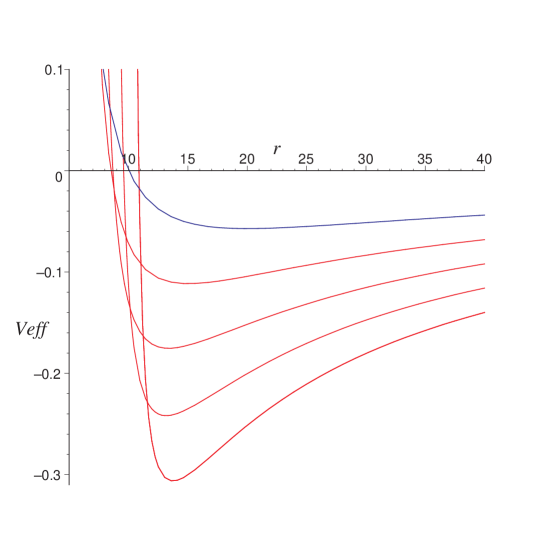
Figure 1: The effective potential for increasing amounts of non–extremality, $r_{0}$. The top curve is the extremal case.

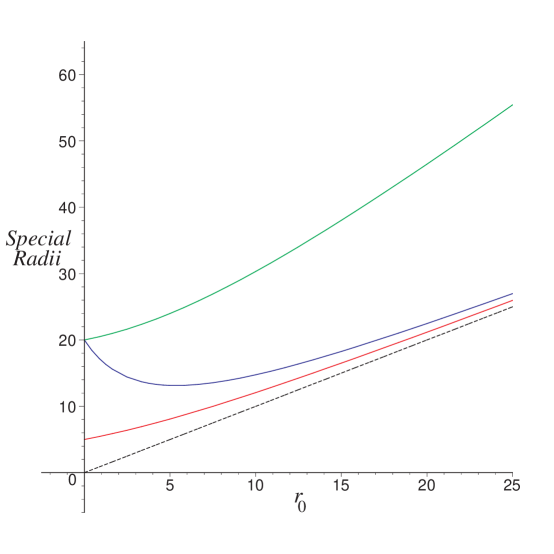
Figure 2: Some special radii for increasing non–extremality, $r_{0}$, in the case $M=0$. The solid curves are as follows: The enhançon radius is top, the repulson radius is bottom, and the minimal radius for which excision would remove all repulsiveness, ${\hat{r}}_{\rm d}$, (which also deserves a name) is the middle curve. Notice that the latter two coalesce into the would–be horizon (dotted line at very bottom) at large $r_{0}$.

The remaining discussion precisely follows that in section 4.2. First, we would say that (unless $M=0$) not all of the D6–branes will stay at the enhançon radius. Rather they will fall into the central black hole until the K3 volume is fixed at $V_{*}$ over this entire region. This condition is determined by precisely the same equation as before, i.e., eqn. (62), which implicitly yields precisely the same constraint as before, $N^{\prime}=N_{*}^{\prime}(r_{0})$. So as before, the physical solution would place $N^{\prime}=N_{*}^{\prime}\mathrel{\hbox to0.0pt{\raise 2.20013pt\hbox{$<$}\hss}{\lower 2.20013pt\hbox{$\sim$}}}M/2$ wrapped D6–branes on the central black hole.

Furthermore our discussion of $r_{0}^{\prime}$ is also as in section 4.2. By examining the transverse stresses in the shell, we argue that we must have $r_{0}^{\prime}<r_{0}$. However, note that in this case, there was no restriction on $r_{0}$, and so we must impose $r_{0}^{\prime}<{\hat{r}}_{\rm e}$ as a separate constraint, which ensures that the central black hole actually fits inside of the enhançon shell. Beyond these two constraints, we have not fixed the final free parameter, $r_{0}^{\prime}$.

5 Concluding Remarks

We have found that a purely supergravity analysis singles out the enhançon radius as a special place in spacetime. For the BPS enhançon, our precise matching calculation was able to verify that the solution proposed in ref. [1] corresponds precisely to introducing a shell of wrapped D6–branes at the enhançon radius. This result shows that the excision procedure suggested by the full string theory is also a sensible construction from the point of view of supergravity. Our analysis also strengthens the case that there is simply a flat–space region inside the enhançon shell (and not, e.g., some breakdown of the spacetime description).

Furthermore, these matching calculations explain why one can sensibly carry out the excision procedure in supergravity, even without full knowledge of the detailed mechanism by which the branes will expand. The latter is especially pertinent to wrapped D$p$–branes with $p\not=6$, where one does not have the intuition supplied by the fact the the expansion is just the physics of ordinary BPS Yang–Mills–Higgs monopoles, and also for uplifts of the enhançon to M–theory, as studied in ref. [14].

It is clear that this technique has wide applications. Some cases of particular interest are Denef’s “empty holes” studied in ref.[15]. There, a similar excision procedure is performed, matching a non–trivial supergravity exterior to a flat space interior. This matching seems to be dictated by supersymmetry and the attractor flow equations. However, the continuity conditions imposed at the excision surface guarantee that the implicit source consists of a shell of massless particles as would be appropriate for a D3–brane wrapping a conifold cycle. It may be interesting to study those solutions from this point of view in more detail.

We used the supergravity analysis to explore a non–extremal deformation of the enhançon. However, in this case, our results seemed less satisfactory, as we were unable to completely fix $r_{0}^{\prime}$, the radius of the black hole in the interior region. Instead we were only able to produce two relatively lax constraints: $r_{0}^{\prime}<r_{0}$ and $r_{0}^{\prime}<{\hat{r}}_{\rm e}$.

In fact, we expect that there is no single correct value for $r_{0}^{\prime}$ in the following sense: The non–extremal configurations consist of two thermal subsystems: the central black hole with the Hawking temperature, and the enhancon shell whose internal degrees of freedom are thermally excited. (We could extend the number of subsystems to three by including a thermal bath at infinity.) While the solution presumably describes these subsystems in thermal equilibrium for one particular value of $r_{0}^{\prime}$, we are implicitly working in a regime where they are only weakly coupled, e.g., thermal fluxes are diffuse enough that their gravitational back reaction is negligible. Hence if the black hole and the enhançon shell have different temperatures, we expect that they will only equilibrate over a very long time span. Hence these static non–extremal solutions can be considered as good approximations to the full system which only evolves very slowly. This would be analogous to how isolated black holes are described by classical solutions of Einstein’s equations and the dynamical effects of Hawking evaporation are ignored. With this reasoning, it is natural to think that $r_{0}^{\prime}$ should remain a free parameter (subject to certain broad constraints) in the non–extremal solutions.

Our partial results with respect to $r_{0}^{\prime}$ provide a good illustration of the fact that the excision technique of matching together different supergravity solutions is a coarse tool when there is no supersymmetry. To completely verify the physical correctness of the results, one must still invoke other arguments. In particular, if the non–extremal solutions are to describe thermally excited enhançons, it seems that we need a better microscopic understanding of the thermal physics of the D–branes in the shell. While it is clear that the R–R sources remain unchanged, i.e., the R–R fields are simply determined by the number of branes, the thermal excitation of the internal modes on the branes will modify the metric and dilaton sources. While the matching calculations allow us to calculate these sources from the supergravity solution for a particular choice of parameters, without a microscopic model we cannot verify, e.g., what the associated temperature should be. In principle, such a microscopic picture would allow us to identify the value of $r_{0}^{\prime}$ at which the central black hole and the enhançon shell would be in thermal equilibrium.

In fact, a larger problem was revealed in examining the non–extremal solutions in the regime where the D6–branes outnumbered the D2–branes. In this case, the solutions exhibit a number of peculiar features. First, the exterior solution never contains an event horizon no matter how large the non–extremality scale $r_{0}$ became. Furthermore, in limit $r_{2}\rightarrow 0$, equivalent to a large K3 volume limit, these solutions do not seem to reproduce the expected non–extremal D6–brane solution. Examining this limit more closely, we see that the R–R 3–form potential actually vanishes at $r_{2}=0$ even though we have a nontrivial harmonic function ${\widehat{H}}_{2}=1-r_{0}/r$. On the other hand, this harmonic function still makes a nontrivial contribution to the metric, and in particular to the dilaton. Hence, rather than the expected solution, we seem to have produced a solution for non–extremal D6–branes carrying some additional dilaton hair. In fact (as in the extremal case), the repulson singularity in these solutions implies that the usual no–hair theorems no longer apply, and so our non–extremal solutions are presumably just one example of a family of singular solutions with the same asymptotic charges and mass, but differing by scalar hair. It would be interesting if these generalised solutions could be found, along the lines of ref. [17], as some of the physical problems might be ameliorated with the appropriate hair dressing. However, without the guidance of supersymmetry in these non–extremal solutions, this seems a daunting task.

Finally, recall our observation that solving the supergravity equations left a sign ambiguity in the following relation:

$$\alpha_{2}r_{2}=\pm\sqrt{r_{2}^{2}+{r_{0}^{2}/4}}-r_{0}/2\ ,$$ (74)

irrespective of the sign of $r_{2}$. In the discussion in section 4, we made the particular choices that the sign is plus (minus) for $M>N$ ($M<N$). Figure 3 illustrates the two different branches in eqn. (74) and our choices in resolving the ambiguity. A feature that distinguishes our choice of signs is that in the limit $r_{0}\to 0$, these two branches coalesce to fill out the diagonal which we know corresponds to the proper BPS solution. However, as illustrated, the two families of solutions actually both extend over the entire range of $M/N$. The solutions on the lower branch are all characterised by having a repulson singularity (before any excision procedure is implemented). As discussed above, these singular solutions are not unique and we will not consider them further here.

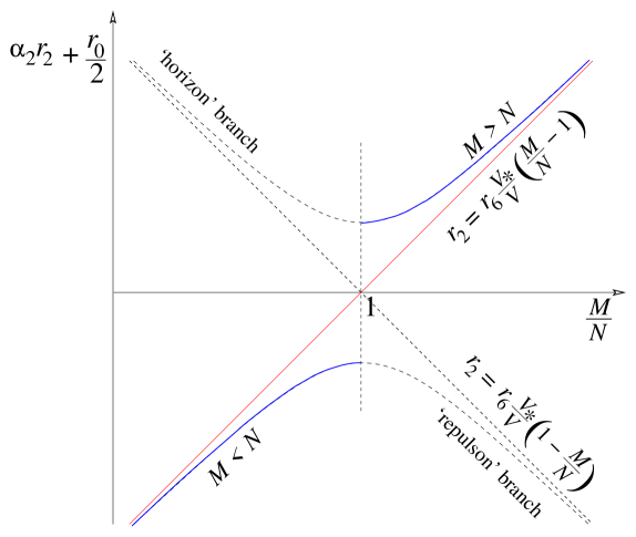
Figure 3: The two branches (solid lines) of supergravity solutions for varying values of the ratio $M/N$. There is a crucial discontinuity at $N=M$. (See text.)

A distinguishing feature of the solutions corresponding to the upper branch is that all of these non–extremal configurations are black holes (again before any excision procedure is implemented). Hence we expect that no–hair theorems will single out these solutions as the unique solutions with a nonsingular event horizon for a given set of parameters: $r_{0}$, $M$ and $N$. Therefore, it is to be expected that there is some interesting physics associated with these solutions even when $M<N$. For example, if we probe a “large” Schwarzschild black hole with either test D6– or D2–brane probes, there are now obstruction to either type of probe from falling into the black hole. So if this black hole absorbs a relatively small number of branes, we expect that the end state must be a black hole in this family of solutions, even if $M<N$. Similarly, one might think about starting with a black hole on the $M>N$ part of this branch and dropping in anti–D2–branes to reduce the final black hole to $M<N$. As a final comment, however, we note that even with small $r_{0}$ the black holes with $M<N$ have masses (relatively) far above the BPS limit.

Acknowledgements

Research by RCM was supported by NSERC of Canada and Fonds FCAR du Québec. Research by AWP was supported by NSERC of Canada and the University of Toronto. Research by CVJ and SFR was partially supported by PPARC of the United Kingdom. We would like to thank the Aspen Center for Physics for hospitality during the initial stages of this project. CVJ would like to thank the ITP at Stanford for hospitality, during the latter stages of this project. AWP would like to thank Emil Martinec, Sumati Surya and Lenny Susskind for useful discussions. RCM would like to thank Neil Constable and Frederik Denef for useful discussions. We thank Joe Polchinski for very useful conversations. CVJ, AWP and SFR would like to thank the ITP in Santa Barbara for hospitality, and the organisers of the M–theory workshop for the opportunity to participate. We thank all of participants of the workshop for remarks. Research at the ITP (Santa Barbara) was supported in part by the U.S. National Science Foundation under Grant No. PHY99–07949.

References

- [1] C. V. Johnson, A. W. Peet and J. Polchinski, “Gauge theory and the excision of repulson singularities”, Phys. Rev. D61 (2000) 086001 [hep-th/9911161].
- [2] K. Behrndt, “About a class of exact string backgrounds”, Nucl. Phys. B455, 188 (1995) [hep-th/9506106].
- [3] R. Kallosh and A. Linde, “Exact supersymmetric massive and massless white holes”, Phys. Rev. D52, 7137 (1995) [hep-th/9507022].
- [4] See also: M. Cvetič and D. Youm, “Singular BPS saturated states and enhanced symmetries of four-dimensional N=4 supersymmetric string vacua”, Phys. Lett. B359, 87 (1995) [hep-th/9507160].
- [5] C.P. Bachas, P. Bain and M.B. Green, “Curvature terms in D-brane actions and their M-theory origin”, JHEP 05, 011 (1999) [hep-th/9903210].
- [6] M. Bershadsky, C. Vafa and V. Sadov, “D-Strings on D-Manifolds”, Nucl. Phys. B463 (1996) 398 [hep-th/9510225].
-
[7]
M.B. Green, J.A. Harvey and G. Moore,
“I-brane inflow and anomalous couplings on D-branes”,
Class. Quant. Grav. 14 (1997) 47 [hep-th/9605033];
Y.E. Cheung and Z. Yin, “Anomalies, branes, and currents”, Nucl. Phys. B517 (1998) 69 [hep-th/9710206]. - [8] K. Dasgupta, D.P. Jatkar and S. Mukhi, “Gravitational couplings and orientifolds”, Nucl. Phys. B523, 465 (1998) [hep-th/9707224].
- [9] C. V. Johnson, “Enhançons, fuzzy spheres and multi-monopoles”, Phys. Rev. D63 (2001) 065004 [hep-th/0004068].
- [10] C. V. Johnson, “The enhançon, multimonopoles and fuzzy geometry”, Int. J. Mod. Phys. A 16, 990 (2001) [hep-th/0011008] (talk at Strings 2000).
- [11] W. Israel, “Singular hypersurfaces and thin shells in general relativity”, Nuovo Cim. 44B (1966) 1.
- [12] C.W. Misner, K.S. Thorne and J.A. Wheeler, Gravitation (San Francisco: Freeman, 1973).
- [13] C. V. Johnson and R. C. Myers, “The Enhançon, Black Holes and the Second Law”, hep-th/0105159.
- [14] L. Järv and C.V. Johnson, “Orientifolds, M-theory, and the ABCD’s of the enhançon”, Phys. Rev. D62 (2000) 126010 [hep-th/0002244].
- [15] F. Denef, “Supergravity flows and D-brane stability”, JHEP 0008 (2000) 050 [hep-th/0005049].
- [16] P. Berglund, T. Hubsch and D. Minic, “Exponential hierarchy from spacetime variable string vacua”, JHEP 0009, 015 (2000) [hep-th/0005162]; “Probing naked singularities in non-supersymmetric string vacua”, JHEP 0102, 010 (2001) [hep-th/0012042]; “On relativistic brane probes in singular spacetimes”, JHEP 0101, 041 (2001) [hep-th/0012180]; “Localized gravity and large hierarchy from string theory?”, hep-th/0104057.
- [17] C.P. Burgess, R.C. Myers and F. Quevedo, “On spherically symmetric string solutions in four-dimensions”, Nucl. Phys. B 442 (1995) 75 [hep-th/9410142]; “Duality and four-dimensional black holes”, Nucl. Phys. B 442 (1995) 97 [hep-th/9411195].