Phase Structure of D-brane Gauge Theories and Toric Duality

Abstract:

Harnessing the unimodular degree of freedom in the definition of any toric diagram, we present a method of constructing inequivalent gauge theories which are world-volume theories of D-branes probing the same toric singularity. These theories are various phases in partial resolution of Abelian orbifolds. As examples, two phases are constructed for both the zeroth Hirzebruch and the second del Pezzo surfaces. We show that such a phenomenon is a special case of “Toric Duality” proposed in hep-th/0003085. Furthermore, we investigate the general conditions that distinguish these different gauge theories with the same (toric) moduli space.

1 Introduction

The methods of toric geometry have been a crucial tool to the understanding of many fundamental aspects of string theory on Calabi-Yau manifolds (cf. e.g. [1]). In particular, the connexions between toric singularities and the manufacturing of various gauge theories as D-brane world-volume theories have been intimate.

Such connexions have been motivated by a myriad of sources. As far back as 1993, Witten [2] had shown, via the so-called gauged linear sigma model, that the Fayet-Illiopoulos parametre $r$ in the D-term of an ${\cal N}=2$ supersymmetric field theory with $U(1)$ gauge groups can be tuned as an order-parametre which extrapolates between the Landau-Ginzburg and Calabi-Yau phases of the theory, whereby giving a precise viewpoint to the LG/CY-correspondence. What this means in the context of Abelian gauge theories is that whereas for $r\ll 0$, we have a Landau-Ginzberg description of the theory, by taking $r\gg 0$, the space of classical vacua obtained from D- and F-flatness is described by a Calabi-Yau manifold, and in particular a toric variety.

With the advent of D-brane technologies, vast amount of work has been done to study the dynamics of world-volume theories on D-branes probing various geometries. Notably, in [3], D-branes have been used to probe Abelian singularities of the form $\hbox{$\,\vrule height=6.45831pt,width=0.4pt,depth=0.0pt\kern-3.00003pt{\rm C}$}^{2}/\mathchoice{\hbox{\cmss Z\kern-3.99994ptZ}}{\hbox{\cmss Z\kern-3.99994ptZ}}{\lower 0.9pt\hbox{\cmsss Z\kern-2.79996ptZ}}{\lower 1.2pt\hbox{\cmsss Z\kern-2.79996ptZ}}_{n}$. Methods of studying the moduli space of the SUSY theories describable by quiver diagrams have been developed by the recognition of the Kronheimer-Nakajima ALE instanton construction, especially the moment maps used therein [4].

Much work followed [5, 6, 7]. A key advance was made in [8], where, exemplifying with Abelian $\hbox{$\,\vrule height=6.45831pt,width=0.4pt,depth=0.0pt\kern-3.00003pt{\rm C}$}^{3}$ orbifolds, a detailed method was developed for capturing the various phases of the moduli space of the quiver gauge theories as toric varieties. In another vein, the huge factory built after the brane-setup approach to gauge theories [9] has been continuing to elucidate the T-dual picture of branes probing singularities (e.g. [10, 11, 12]). Brane setups for toric resolutions of $\mathchoice{\hbox{\cmss Z\kern-3.99994ptZ}}{\hbox{\cmss Z\kern-3.99994ptZ}}{\lower 0.9pt\hbox{\cmsss Z\kern-2.79996ptZ}}{\lower 1.2pt\hbox{\cmsss Z\kern-2.79996ptZ}}_{2}\times\mathchoice{\hbox{\cmss Z\kern-3.99994ptZ}}{\hbox{\cmss Z\kern-3.99994ptZ}}{\lower 0.9pt\hbox{\cmsss Z\kern-2.79996ptZ}}{\lower 1.2pt\hbox{\cmsss Z\kern-2.79996ptZ}}_{2}$, including the famous conifold, were addressed in [17, 18]. The general question of how to construct the quiver gauge theory for an arbitrary toric singularity was still pertinent. With the AdS/CFT correspondence emerging [5, 6], the pressing need for the question arises again: given a toric singularity, how does one determine the quiver gauge theory having the former as its moduli space?

The answer lies in “Partial Resolution of Abelian Orbifolds” and was introduced and exemplified for the toric resolutions of the $\mathchoice{\hbox{\cmss Z\kern-3.99994ptZ}}{\hbox{\cmss Z\kern-3.99994ptZ}}{\lower 0.9pt\hbox{\cmsss Z\kern-2.79996ptZ}}{\lower 1.2pt\hbox{\cmsss Z\kern-2.79996ptZ}}_{3}\times\mathchoice{\hbox{\cmss Z\kern-3.99994ptZ}}{\hbox{\cmss Z\kern-3.99994ptZ}}{\lower 0.9pt\hbox{\cmsss Z\kern-2.79996ptZ}}{\lower 1.2pt\hbox{\cmsss Z\kern-2.79996ptZ}}_{3}$ orbifold [8, 13]. The method was subsequently presented in an algorithmic and computationally feasible fashion in [14] and was applied to a host of examples in [15].

One short-coming about the inverse procedure of going from the toric data to the gauge theory data is that it is highly non-unique and in general, unless one starts by partially resolving an orbifold singularity, one would not be guaranteed with a physical world-volume theory at all! Though the non-uniqueness was harnessed in [14] to construct families of quiver gauge theories with the same toric moduli space, a phenomenon which was dubbed “toric duality,” the physicality issue remains to be fully tackled.

The purpose of this writing is to analyse toric duality within the confinement of the canonical method of partial resolutions. Now we are always guaranteed with a world-volume theory at the end and this physicality is of great assurance to us. We find indeed that with the restriction of physical theories, toric duality is still very much at work and one can construct D-brane quiver theories that flow to the same moduli space.

We begin in §2 with a seeming paradox which initially motivated our work and which ab initio appeared to present a challenge to the canonical method. In §3 we resolve the paradox by introducing the well-known mathematical fact of toric isomorphisms. Then in §4, we present a detailed analysis, painstakingly tracing through each step of the inverse procedure to see how much degree of freedom one is allowed as one proceeds with the algorithm. We consequently arrive at a method of extracting torically dual theories which are all physical; to these we refer as “phases.” As applications of these ideas in §5 we re-analyse the examples in [14], viz., the toric del Pezzo surfaces as well as the zeroth Hirzebruch surface and find the various phases of the quiver gauge theories with them as moduli spaces. Finally in §6 we end with conclusions and future prospects.

2 A Seeming Paradox

In [14] we noticed the emergence of the phenomenon of “Toric Duality” wherein the moduli space of vast numbers of gauge theories could be parametrised by the same toric variety. Of course, as we mentioned there, one needs to check extensively whether these theories are all physical in the sense that they are world-volume theories of some D-brane probing the toric singularity.

Here we shall discuss an issue of more immediate concern to the physical probe theory. We recall that using the method of partial resolutions of Abelian orbifolds [14, 8, 13, 17], we could always extract a canonical theory on the D-brane probing the singularity of interest.

However, a discrepancy of results seems to have risen between [14] and [6] on the precise world-volume theory of a D-brane probe sitting on the zeroth Hirzebruch surface; let us compare and contrast the two results here.

• Results from [14]: The matter contents of the theory are given by (on the left we present the quiver diagram and on the right, the incidence matrix that encodes the quiver):

  $$\begin{array}[]{lcr}\mbox{ \epsfbox{quiverF0_1} }&&d=\left(\matrix{\begin{array}[]{c|cccccccccccc}&X_{1}&X_{2}&X_{3}&X_{4}&X_{5}&X_{6}&X_{7}&X_{8}&X_{9}&X_{10}&X_{11}&X_{12}\\ \hline\cr A&-1&0&-1&0&-1&0&1&1&-1&0&1&1\\ B&0&-1&0&-1&1&0&0&0&1&0&0&0\\ C&0&1&0&1&0&1&-1&-1&0&1&-1&-1\\ D&1&0&1&0&0&-1&0&0&0&-1&0&0\end{array}}\right)\end{array}$$

  and the superpotential is given by

  $$W=X_{1}X_{8}X_{10}-X_{3}X_{7}X_{10}-X_{2}X_{8}X_{9}-X_{1}X_{6}X_{12}+\\ X_{3}X_{6}X_{11}+X_{4}X_{7}X_{9}+X_{2}X_{5}X_{12}-X_{4}X_{5}X_{11}.$$ (2.1)

• Results from [6]: The matter contents of the theory are given by (for $i=1,2$):

  $$\begin{array}[]{lcr}\epsfbox{quiverF0_2}&&d=\left(\matrix{\begin{array}[]{c|cccc}&X_{i~{}12}&X_{i~{}21}&Y_{i~{}11}&Y_{i~{}22}\\ \hline\cr A&-1&0&1&0\\ B&1&0&0&-1\\ C&0&1&-1&0\\ D&0&-1&0&1\\ \end{array}}\right)\end{array}$$

  and the superpotential is given by

  $$W=\epsilon^{ij}\epsilon^{kl}X_{i~{}12}Y_{k~{}22}X_{j~{}21}Y_{l~{}11}.$$ (2.2)

Indeed, even though both these theories have arisen from the canonical partial resolutions technique and hence are world volume theories of a brane probing a Hirzebruch singularity, we see clearly that they differ vastly in both matter content and superpotential! Which is the “correct” physical theory?

In response to this seeming paradox, let us refer to Figure 1.

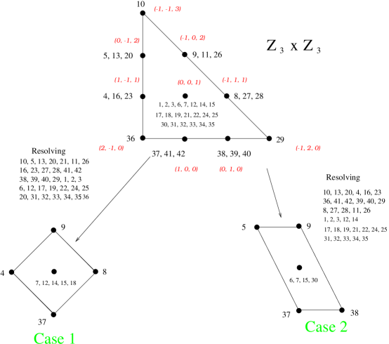
Figure 1: Two alternative resolutions of $\hbox{$\,\vrule height=6.45831pt,width=0.4pt,depth=0.0pt\kern-3.00003pt{\rm C}$}^{2}/\mathchoice{\hbox{\cmss Z\kern-3.99994ptZ}}{\hbox{\cmss Z\kern-3.99994ptZ}}{\lower 0.9pt\hbox{\cmsss Z\kern-2.79996ptZ}}{\lower 1.2pt\hbox{\cmsss Z\kern-2.79996ptZ}}_{3}\times\mathchoice{\hbox{\cmss Z\kern-3.99994ptZ}}{\hbox{\cmss Z\kern-3.99994ptZ}}{\lower 0.9pt\hbox{\cmsss Z\kern-2.79996ptZ}}{\lower 1.2pt\hbox{\cmsss Z\kern-2.79996ptZ}}_{3}$ to the Hirzebruch surface $F_{0}$: Case 1 from [14] and Case 2 from [6].

Case 1 of course was what had been analysed in [14] (q.v. ibid.) and presented in (2.1); let us now consider case 2. Using the canonical algorithm of [13, 14], we obtain the matter content (we have labelled the fields and gauge groups with some foresight)

$$d_{ia}=\left(\begin{array}[]{c|cccccccc}&X_{1}&X^{\prime}_{1}&X^{\prime}_{2}&Y_{1}&Y_{2}&Y^{\prime}_{1}&Y_{2}&Y^{\prime}_{2}\\ \hline\cr D&0&1&1&0&0&-1&0&-1\\ A&-1&0&0&1&1&0&-1&0\\ B&1&-1&-1&0&0&0&1&0\\ C&0&0&0&-1&-1&1&0&1\end{array}\right)$$

and the dual cone matrix

$$K_{ij}^{T}=\left(\begin{array}[]{c|cccccccc}&X_{1}&X^{\prime}_{1}&X^{\prime}_{2}&Y_{1}&Y_{2}&Y^{\prime}_{1}&X_{2}&Y^{\prime}_{2}\\ \hline\cr p_{1}&1&0&0&0&0&1&0&0\\ p_{2}&0&1&0&1&0&0&0&0\\ p_{3}&1&0&0&0&0&0&1&0\\ p_{4}&0&1&1&0&0&0&0&0\\ p_{5}&0&0&1&0&1&0&0&0\\ p_{6}&0&0&0&0&0&1&0&1\end{array}\right)$$

which translates to the F-term equations

$$X_{1}Y^{\prime}_{2}=p_{1}p_{3}p_{6}=Y^{\prime}_{1}X_{2};\quad X^{\prime}_{1}Y_{2}=p_{2}p_{4}p_{5}=Y_{1}X^{\prime}_{2}.$$

What we see of course, is that with the field redefinition $X_{i}\leftrightarrow X_{i~{}12},X^{\prime}_{i}\leftrightarrow Y_{i~{}22},Y_{i}\leftrightarrow Y_{i~{}11}$ and $Y^{\prime}_{i}\leftrightarrow X_{i~{}21}$ for $i=1,2$, the above results are in exact agreement with the results from [6] as presented in (2.2).

This is actually of no surprise to us because upon closer inspection of Figure 1, we see that the toric diagram for Cases 1 and 2 respectively has the coordinate points

$$G1_{t}=\left(\matrix{-1&1&1&0&-1\cr 0&-1&0&0&1\cr 2&1&0&1&1\cr}\right)\qquad G2_{t}=\left(\matrix{0&-1&1&0&0\cr-1&0&0&1&0\cr 2&2&0&0&1\cr}\right).$$

Now since the algebraic equation of the toric variety is given by [19]

$$V(G_{t})=Spec_{Max}\left({\mathchoice{{\kern 2.70004pt\vrule height=6.24301pt,width=0.29999pt,depth=0.0pt\kern-3.00003pt\rm C}}{{\kern 2.70004pt\vrule height=6.24301pt,width=0.29999pt,depth=0.0pt\kern-3.00003pt\rm C}}{\kern 2.25006pt\vrule height=4.52083pt,width=0.24994pt,depth=0.0pt\kern-2.5pt\rm C}{\kern 1.79993pt\vrule height=3.3583pt,width=0.20004pt,depth=0.0pt\kern-1.99997pt\rm C}}[X_{i}^{G_{t}^{\vee}\cap\mathchoice{\hbox{\cmss Z\kern-3.99994ptZ}}{\hbox{\cmss Z\kern-3.99994ptZ}}{\lower 0.9pt\hbox{\cmsss Z\kern-2.79996ptZ}}{\lower 1.2pt\hbox{\cmsss Z\kern-2.79996ptZ}}^{3}}]\right),$$

we have checked that, using a reduced Gröbner polynomial basis algorithm to compute the variety [20], the equations are identical up to redefinition of variables.

Therefore we see that the two toric diagrams in Cases 1 and 2 of Figure 1 both describe the zeroth Hirzebruch surface as they have the same equations (embedding into $\hbox{$\,\vrule height=6.45831pt,width=0.4pt,depth=0.0pt\kern-3.00003pt{\rm C}$}^{9}$). Yet due to the particular choice of the diagram, we end up with strikingly different gauge theories on the D-brane probe despite the identification of the moduli space in the IR. This is indeed a curiously strong version of “toric duality.”

Bearing the above in mind, in this paper, we will analyse the degrees of freedom in the Inverse Algorithm expounded upon in [14], i.e., for a given toric singularity, how many different physical gauge theories (phase structures), resulting from various partial resolutions can one have for a D-brane probing such a singularity? To answer this question, first in §2 we present the concept of toric isomorphism and give the conditions for different toric data to correspond to the same toric variety. Then in §3 we follow the Forward Algorithm and give the freedom at each step from a given set of gauge theory data all the way to the output of the toric data. Knowing these freedoms, we can identify the sources that may give rise to different gauge theories in the Inverse Algorithm starting from a prescribed toric data. In section 4, we apply the above results and analyse the different phases for the partial resolutions of the $\mathchoice{\hbox{\cmss Z\kern-3.99994ptZ}}{\hbox{\cmss Z\kern-3.99994ptZ}}{\lower 0.9pt\hbox{\cmsss Z\kern-2.79996ptZ}}{\lower 1.2pt\hbox{\cmsss Z\kern-2.79996ptZ}}_{3}\times\mathchoice{\hbox{\cmss Z\kern-3.99994ptZ}}{\hbox{\cmss Z\kern-3.99994ptZ}}{\lower 0.9pt\hbox{\cmsss Z\kern-2.79996ptZ}}{\lower 1.2pt\hbox{\cmsss Z\kern-2.79996ptZ}}_{3}$ orbifold singularity, in particular, we found that there are two inequivalent phases of gauge theories respectively for the zeroth Hirzebruch surface and the second del Pezzo surface. Finally, in section 5, we give discussions for further investigation.

3 Toric Isomorphisms

Extending this observation to generic toric singularities, we expect classes of inequivalent toric diagrams corresponding to the same variety to give rise to inequivalent gauge theories on the D-brane probing the said singularity. An immediate question is naturally posed: “is there a classification of these different theories and is there a transformation among them?”

To answer this question we resort to the following result. Given $M$-lattice cones $\sigma$ and $\sigma^{\prime}$, let the linear span of $\sigma$ be lin$\sigma={\rm I\kern-1.79993ptR}^{n}$ and that of $\sigma^{\prime}$ be ${\rm I\kern-1.79993ptR}^{m}$. Now each cone gives rise to a semigroup which is the intersection of the dual cone $\sigma^{\vee}$ with the dual lattice $M$, i.e., $S_{\sigma}:=\sigma^{\vee}\cap M$ (likewise for $\sigma^{\prime}$). Finally the toric variety is given as the maximal spectrum of the polynomial ring of $\,\vrule height=6.45831pt,width=0.4pt,depth=0.0pt\kern-3.00003pt{\rm C}$ adjoint the semigroup, i.e., $X_{\sigma}:=Spec_{Max}\left(\hbox{$\,\vrule height=6.45831pt,width=0.4pt,depth=0.0pt\kern-3.00003pt{\rm C}$}[S_{\sigma}]\right)$.

DEFINITION 3.1

We have these types of isomorphisms:

1. We call $\sigma$ and $\sigma^{\prime}$ cone isomorphic, denoted $\sigma\cong_{cone}\sigma^{\prime}$, if $n=m$ and there is a unimodular transformation $L:{\rm I\kern-1.79993ptR}^{n}\rightarrow{\rm I\kern-1.79993ptR}^{n}$ with $L(\sigma)=\sigma^{\prime}$;

2. we call $S_{\sigma}$ and $S_{\sigma^{\prime}}$ monomial isomorphic, denoted $S_{\sigma}\cong_{mon}S_{\sigma^{\prime}}$, if there exists mutually inverse monomial homomorphisms between the two semigroups.

Thus equipped, we are endowed with the following

THEOREM 3.1

([22], VI.2.11) The following conditions are equivalent:

$$(a)~{}~{}\sigma\cong_{cone}\sigma^{\prime}\Leftrightarrow(b)~{}~{}S_{\sigma}\cong_{mon}S_{\sigma^{\prime}}\Leftrightarrow(c)~{}~{}X_{\sigma}\cong X_{\sigma^{\prime}}$$

What this theorem means for us is simply that, for the $n$-dimensional toric variety, an $SL(n;\mathchoice{\hbox{\cmss Z\kern-3.99994ptZ}}{\hbox{\cmss Z\kern-3.99994ptZ}}{\lower 0.9pt\hbox{\cmsss Z\kern-2.79996ptZ}}{\lower 1.2pt\hbox{\cmsss Z\kern-2.79996ptZ}})$ transformation on the original lattice cone amounts to merely coördinate transformations on the polynomial ring and results in the same toric variety. This, is precisely what we want: different toric diagrams giving the same variety.

The necessity and sufficiency of the condition in Theorem 3.1 is important. Let us think of one example to illustrate. Let a cone be defined by $(e_{1},e_{2})$, we know this corresponds to $\hbox{$\,\vrule height=6.45831pt,width=0.4pt,depth=0.0pt\kern-3.00003pt{\rm C}$}^{2}$. Now if we apply the transformation

$$(e_{1},e_{2})\left[\begin{array}[]{cc}2&0\\ -1&1\end{array}\right]=(2e_{1}-e_{2},e_{2}),$$

which corresponds to the variety $xy=z^{2}$, i.e., $\hbox{$\,\vrule height=6.45831pt,width=0.4pt,depth=0.0pt\kern-3.00003pt{\rm C}$}^{2}/\mathchoice{\hbox{\cmss Z\kern-3.99994ptZ}}{\hbox{\cmss Z\kern-3.99994ptZ}}{\lower 0.9pt\hbox{\cmsss Z\kern-2.79996ptZ}}{\lower 1.2pt\hbox{\cmsss Z\kern-2.79996ptZ}}_{2}$, which of course is not isomorphic to $\hbox{$\,\vrule height=6.45831pt,width=0.4pt,depth=0.0pt\kern-3.00003pt{\rm C}$}^{2}$. The reason for this is obvious: the matrix we have chosen is certainly not unimodular.

4 Freedom and Ambiguity in the Algorithm

In this section, we wish to step back and address the issue in fuller generality. Recall that the procedure of obtaining the moduli space encoded as toric data once given the gauge theory data in terms of product $U(1)$ gauge groups, D-terms from matter contents and F-terms from the superpotential, has been well developed [6, 8]. Such was called the forward algorithm in [14]. On the other hand the reverse algorithm of obtaining the gauge theory data from the toric data has been discussed extensively in [13, 14].

It was pointed in [14] that both the forward and reverse algorithm are highly non-unique, a property which could actually be harnessed to provide large classes of gauge theories having the same IR moduli space. In light of this so-named “toric duality” it would be instructive for us to investigate how much freedom do we have at each step in the algorithm. We will call two data related by such a freedom equivalent to each other. Thence further we could see how freedoms at every step accumulate and appear in the final toric data. Modulo such equivalences we believe that the data should be uniquely determinable.

4.1 The Forward Algorithm

We begin with the forward algorithm of extracting toric data from gauge data. A brief review is at hand. To specify the gauge theory, we require three pieces of information: the number of $U(1)$ gauge fields, the charges of matter fields and the superpotential. The first two are summarised by the so-called charge matrix $d_{li}$ where $l=1,2,...,L$ with $L$ the number of $U(1)$ gauge fields and $i=1,2,...,I$ with $I$ the number of matter fields. When using the forward algorithm to find the vacuum manifold (as a toric variety), we need to solve the D-term and F-term flatness equations. The D-terms are given by $d_{li}$ matrix while the F-terms are encoded in a matrix $K_{ij}$ with $i,1,2,...,I$ and $j=1,2,...,J$ where $J$ is the number of independent parameters needed to solve the F-terms. By gauge data then we mean the matrices $d$ (also called the incidence matrix) and the $K$ (essentially the dual cone); the forward algorithm takes these as input. Subsequently we trace a flow-chart:

$$\begin{array}[]{ccccccc}\mbox{D-Terms}\rightarrow d&\rightarrow&\Delta&&&&\\ &&\downarrow&&&&\\ \mbox{F-Terms}\rightarrow K&\stackrel{{\scriptstyle V\cdot K^{T}=\Delta}}{{\rightarrow}}&V&&&&\\ \downarrow&&\downarrow&&&&\\ T={\rm Dual}(K)&\stackrel{{\scriptstyle U\cdot T^{T}={\rm Id}}}{{\rightarrow}}&U&\rightarrow&VU&&\\ \downarrow&&&&\downarrow&&\\ Q=[{\rm Ker}(T)]^{T}&&\longrightarrow&&Q_{t}=\left(\begin{array}[]{c}Q\\ VU\end{array}\right)&\rightarrow&G_{t}=[{\rm Ker}(Q_{t})]^{T}\\ \end{array}$$

arriving at a final matrix $G_{t}$ whose columns are the vectors which prescribe the nodes of the toric diagram.

What we wish to investigate below is how much procedural freedom we have at each arrow so as to ascertain the non-trivial toric dual theories. Hence, if $A_{1}$ is the matrix whither one arrives from a certain arrow, then we would like to find the most general transformation taking $A_{1}$ to another solution $A_{2}$ which would give rise to an identical theory. It is to this transformation that we shall refer as “freedom” at the particular step.

Superpotential: the matrices $K$ and $T$

The solution of F-term equations gives rise to a dual cone $K_{1}=K_{ij}$ defined by $I$ vectors in $\mathchoice{\hbox{\cmss Z\kern-3.99994ptZ}}{\hbox{\cmss Z\kern-3.99994ptZ}}{\lower 0.9pt\hbox{\cmsss Z\kern-2.79996ptZ}}{\lower 1.2pt\hbox{\cmsss Z\kern-2.79996ptZ}}^{J}$. Of course, we can choose different parametres to solve the F-terms and arrive at another dual cone $K_{2}$. Then, $K_{1}$ and $K_{2}$, being integral cones, are equivalent if they are unimodularly related, i.e., $K_{2}^{T}=A\cdot K_{1}^{T}$ for $A\in GL(J,\mathchoice{\hbox{\cmss Z\kern-3.99994ptZ}}{\hbox{\cmss Z\kern-3.99994ptZ}}{\lower 0.9pt\hbox{\cmsss Z\kern-2.79996ptZ}}{\lower 1.2pt\hbox{\cmsss Z\kern-2.79996ptZ}})$ such that $\det(A)=\pm 1$. Furthermore, the order of the $I$ vectors in $\mathchoice{\hbox{\cmss Z\kern-3.99994ptZ}}{\hbox{\cmss Z\kern-3.99994ptZ}}{\lower 0.9pt\hbox{\cmsss Z\kern-2.79996ptZ}}{\lower 1.2pt\hbox{\cmsss Z\kern-2.79996ptZ}}^{J}$ clearly does not matter, so we can permute them by a matrix $S_{I}$ in the symmetric group ${\cal S}_{I}$. Thus far we have two freedoms, multiplication by $A$ and $S$:

$$K_{2}^{T}=A\cdot K_{1}^{T}\cdot S_{I},$$ (4.3)

and $K_{1,2}$ should give equivalent theories.

Now, from $K_{ij}$ we can find its dual matrix $T_{j\alpha}$ (defining the cone $T$) where $\alpha=1,2,...,c$ and $c$ is the number of vectors of the cone $T$ in $\mathchoice{\hbox{\cmss Z\kern-3.99994ptZ}}{\hbox{\cmss Z\kern-3.99994ptZ}}{\lower 0.9pt\hbox{\cmsss Z\kern-2.79996ptZ}}{\lower 1.2pt\hbox{\cmsss Z\kern-2.79996ptZ}}^{J}$, as constrained by

$$K\cdot T\geq 0$$ (4.4)

and such that $T$ also spans an integral cone. Notice that finding dual cones, as given in a algorithm in [19], is actually unique up to permutation of the defining vectors. Now considering the freedom of $K_{ij}$ as in (4.3), let $T_{2}$ be the dual of $K_{2}$ and $T_{1}$ that of $K_{1}$, we have $K_{2}\cdot T_{2}=S_{I}^{T}\cdot K_{1}\cdot A^{T}\cdot T_{2}\geq 0$, which means that

$$T_{1}=A^{T}\cdot T_{2}\cdot S_{c}.$$ (4.5)

Note that here $S_{c}$ is the permutation of the $c$ vectors of the cone $T$ in and not that of the dual cone in (4.3).

The Charge Matrix $Q$

The next step is to find the charge matrix $Q_{k\alpha}$ where $\alpha=1,2,...,c$ and $k=1,2,...,c-J$. This matrix is defined by

$$T\cdot Q^{T}=0.$$ (4.6)

In the same spirit as the above discussion, from (4.5) we have $T_{1}\cdot Q_{1}^{T}=A^{T}\cdot T_{2}\cdot S_{c}\cdot Q_{1}^{T}=0$. Because $A^{T}$ is a invertible matrix, this has a solution when and only when $T_{2}\cdot S_{c}\cdot Q_{1}^{T}=0$. Of course this is equivalent to $T_{2}\cdot S_{c}\cdot Q_{1}^{T}\cdot B_{kk^{\prime}}=0$ for some invertible $(c-J)\times(c-J)$ matrix $B_{kk^{\prime}}$. So the freedom for matrix $Q$ is

$$Q_{2}^{T}=S_{c}\cdot Q_{1}^{T}\cdot B.$$ (4.7)

We emphasize a difference from (4.4); there we required both matrices $K$ and $T$ to be integer where here (4.6) does not possess such a constraint. Thus the only condition for the matrix $B$ is its invertibility.

Matter Content: the Matrices $d$, $\widetilde{V}$ and $U$

Now we move onto the D-term and the integral $d_{li}$ matrix. The D-term equations are $d\cdot|X|^{2}=0$ for matter fields $X$. Obviously, any transformation on $d$ by an invertible matrix $C_{L\times L}$ does not change the D-terms. Furthermore, any permutation $S_{I}$ of the order the fields $X$, so long as it is consistent with the $S_{I}$ in (4.3), is also game. In other words, we have the freedom:

$$d_{2}=C\cdot d_{1}\cdot S_{I}.$$ (4.8)

We recall that a matrix $V$ is then determined from $\Delta$, which is $d$ with a row deleted due to the centre of mass degree of freedom. However, to not to spoil the above freedom enjoyed by matrix $d$ in (4.8), we will make a slight amendment and define the matrix $\widetilde{V}_{lj}$ by

$$\widetilde{V}\cdot K^{T}=d.$$ (4.9)

Therefore, whereas in [8, 14] where $V\cdot K^{T}=\Delta$ was defined, we generalise $V$ to $\widetilde{V}$ by (4.9). One obvious way to obtain $\widetilde{V}$ from $V$ is to add one row such that the sum of every column is zero. However, there is a caveat: when there exists a vector $h$ such that

$$h\cdot K^{T}=0,$$

we have the freedom to add $h$ to any row of $\widetilde{V}$. Thus finding the freedom of $\widetilde{V}_{lj}$ is a little more involved. From (4.3) we have $d_{2}=\widetilde{V}_{2}\cdot K_{2}^{T}=\widetilde{V}_{2}\cdot A\cdot K_{1}^{T}\cdot S_{I}$ and $d_{2}=C\cdot d_{1}\cdot S_{I}=C\cdot\widetilde{V}_{1}\cdot K_{1}^{T}\cdot S_{I}$. Because $S_{I}$ is an invertible square matrix, we have $(\widetilde{V}_{2}\cdot A-C\cdot\widetilde{V}_{1})\cdot K_{1}^{T}=0$, which means $\widetilde{V}_{2}\cdot A-C\cdot\widetilde{V}_{1}=CH_{K_{1}}$ for a matrix $H$ constructed by having the aforementioned vectors $h$ as its columns. When $K^{T}$ has maximal rank, $H$ is zero and this is in fact the more frequently encountered situation. However, when $K^{T}$ is not maximal rank, so as to give non-trivial solutions of $h$, we have that $\widetilde{V}_{1}$ and $\widetilde{V}_{2}$ are equivalent if

$$\widetilde{V}_{2}=C\cdot(\widetilde{V}_{1}+H_{K_{1}})\cdot A^{-1}.$$ (4.10)

Moving on to the matrix $U_{j\alpha}$ defined by

$$U\cdot T^{T}={\rm I\kern-1.79993ptI}_{jj^{\prime}},$$ (4.11)

we have from (4.5) ${\rm I\kern-1.79993ptI}_{jj^{\prime}}=U_{1}\cdot T_{1}^{T}=U_{1}\cdot S_{c}^{T}\cdot T_{2}^{T}\cdot A$, whence $A^{-1}=U_{1}\cdot S_{c}^{T}\cdot T_{2}^{T}$ and ${\rm I\kern-1.79993ptI}=A\cdot U_{1}\cdot S_{c}^{T}\cdot T_{2}^{T}$. This gives $(A\cdot U_{1}\cdot S_{c}^{T}-U_{2})\cdot T_{2}^{T}=0$ which has a solution $A\cdot U_{1}\cdot S_{c}^{T}-U_{2}=H_{T_{2}}$ where $H_{T_{2}}\cdot T_{2}^{T}=0$ is precisely as defined in analogy of the $H$ above. Therefore the freedom on $U$ is subsequently

$$U_{2}=A\cdot(U_{1}-H_{T_{1}})\cdot S_{c}^{T},$$ (4.12)

where $H_{T_{1}}=A^{-1}H_{T_{2}}(S_{c}^{T})^{-1}$ and $H_{T_{1}}\cdot T^{T}_{1}=(A^{-1}H_{T_{2}}(S_{c}^{T})^{-1})(S_{c}^{T}\cdot T_{2}^{T}\cdot A)=0$. Finally using (4.10) and (4.12), we have

$$(\widetilde{V}_{2}\cdot U_{2})=C\cdot(\widetilde{V}_{1}+H_{K_{1}})\cdot A^{-1}\cdot A\cdot(U_{1}-H_{T_{1}})\cdot S_{c}^{T}=C\cdot(\widetilde{V}_{1}+H_{K_{1}})(U_{1}-H_{T_{1}})\cdot S_{c}^{T},$$ (4.13)

determining the freedom of the relevant combination $(\widetilde{V}\cdot U)$.

Let us pause for an important observation that in most cases $H_{K_{1}}=0$, as we shall see in the examples later. From (4.6), which propounds the existence of a non-trivial nullspace for $T$, we see that one can indeed obtain a non-trivial $H_{T_{1}}$ in terms of the combinations of the rows of the charge matrix $Q$, whereby simplifying (4.13) to

$$(\widetilde{V}_{2}\cdot U_{2})=C\cdot(\widetilde{V}_{1}\cdot U_{1}+H_{VU_{1}})\cdot S_{c}^{T},$$ (4.14)

where every row of $H_{VU_{1}}$ is linear combination of rows of $Q_{1}$ and the sum of its columns is zero.

Toric Data: the Matrices $Q_{t}$ and $G_{t}$

At last we come to $\widetilde{Q}_{t}$, which is given by adjoining $Q$ and $\widetilde{V}\cdot U$. The freedom is of course, by combining all of our results above,

$$(\widetilde{Q}_{t})_{2}=\left(\begin{array}[]{c}Q_{2}\\ \widetilde{V}_{2}\cdot U_{2}\end{array}\right)=\left(\begin{array}[]{c}B^{T}\cdot Q_{1}\cdot S_{c}^{T}\\ C\cdot(\widetilde{V}_{1}\cdot U_{1}+H_{VU_{1}})\cdot S_{c}^{T}\end{array}\right)=\left(\begin{array}[]{c}B^{T}\cdot Q_{1}\\ C\cdot(\widetilde{V}_{1}\cdot U_{1}+H_{VU_{1}})\end{array}\right)\cdot S_{c}^{T}$$ (4.15)

Now $\widetilde{Q}_{t}$ determines the nodes of the toric diagram $(G_{t})_{p\alpha}$ ($p=1,2,..,(c-(L-1)-J)$ and $\alpha=1,2,...,c$) by

$$Q_{t}\cdot G_{t}^{T}=0;$$ (4.16)

The columns of $G_{t}$ then describes the toric diagram of the algebraic variety for the vacuum moduli space and is the output of the algorithm. From (4.16) and (4.15) we find that if $(\widetilde{Q}_{t})_{1}\cdot(G_{t})_{1}^{T}=0$, i.e., $Q_{1}\cdot(G_{t})_{1}^{T}=0$ and $\widetilde{V}_{1}\cdot U_{1}\cdot(G_{t})_{1}^{T}=0,$ we automatically have the freedom $(\widetilde{Q}_{t})_{2}\cdot(S_{c}^{T})^{-1}\cdot(\widetilde{G}_{t})_{1}^{T}=0$. This means that at most we can have

$$(G_{t})_{2}^{T}=(S_{c}^{T})^{-1}\cdot(G_{t})_{1}^{T}\cdot D,$$ (4.17)

where $D$ is a $GL(c-(L-1)-J,\mathchoice{\hbox{\cmss Z\kern-3.99994ptZ}}{\hbox{\cmss Z\kern-3.99994ptZ}}{\lower 0.9pt\hbox{\cmsss Z\kern-2.79996ptZ}}{\lower 1.2pt\hbox{\cmsss Z\kern-2.79996ptZ}})$ matrix with $\det(D)=\pm 1$ which is exactly the unimodular freedom for toric data as given by Theorem 3.1.

One immediate remark follows. From (4.16) we obtain the nullspace of $Q_{t}$ in $\mathchoice{\hbox{\cmss Z\kern-3.99994ptZ}}{\hbox{\cmss Z\kern-3.99994ptZ}}{\lower 0.9pt\hbox{\cmsss Z\kern-2.79996ptZ}}{\lower 1.2pt\hbox{\cmsss Z\kern-2.79996ptZ}}^{c}$. It seems that we can choose an arbitrary basis so that $D$ is a $GL(c-(L-1)-J,\mathchoice{\hbox{\cmss Z\kern-3.99994ptZ}}{\hbox{\cmss Z\kern-3.99994ptZ}}{\lower 0.9pt\hbox{\cmsss Z\kern-2.79996ptZ}}{\lower 1.2pt\hbox{\cmsss Z\kern-2.79996ptZ}})$ matrix with the only condition that $\det(D)\neq 0$. However, this is not stringent enough: in fact, when we find cokernel $G_{t}$, we need to find the integer basis for the null space, i.e., we need to find the basis such that any integer null vector can be decomposed into a linear combination of the columns of $G_{t}$. If we insist upon such a choice, the only remaining freedom is that $\det(D)=\pm 1$, viz, unimodularity.

4.2 Freedom and Ambiguity in the Reverse Algorithm

Having analysed the equivalence conditions in last subsection, culminating in (4.15) and (4.17), we now proceed in the opposite direction and address the ambiguities in the reverse algorithm.

The Toric Data: $G_{t}$

We note that the $G_{t}$ matrix produced by the forward algorithm is not minimal in the sense that certain columns are repeated, which after deletion, constitute the toric diagram. Therefore, in our reverse algorithm, we shall first encounter such an ambiguity in deciding which columns to repeat when constructing $G_{t}$ from the nodes of the toric diagram. This so-called repetition ambiguity was discussed in [14] and different choices of repetition may indeed give rise to different gauge theories. It was pointed out (loc. cit.) that arbitrary repetition of the columns certainly does not guarantee physicality. By physicality we mean that the gauge theory arrived at the end of the day should be physical in the sense of still being a D-brane world-volume theory. What we shall focus here however, is the inherent symmetry in the toric diagram, given by (4.17), that gives rise to the same theory. This is so that we could find truly inequivalent physical gauge theories not related by such a transformation as (4.17).

The Charge Matrix: from $G_{t}$ to $Q_{t}$

From (4.16) we can solve for $Q_{t}$. However, for a given $G_{t}$, in principle we can have two solutions $(Q_{t})_{1}$ and $(Q_{t})_{2}$ related by

$$(Q_{t})_{2}=P(Q_{t})_{1},$$ (4.18)

where $P$ is a $p\times p$ matrix with $p$ the number of rows of $Q_{t}$. Notice that the set of such transformations $P$ is much larger than the counterpart in the forward algorithm given in (4.15). This is a second source of ambiguity in the reverse algorithm. More explicitly, we have the freedom to arbitrarily divide the $Q_{t}$ into two parts, viz., the D-term part $\widetilde{V}U$ and the F-term part $Q$. Indeed one may find a matrix $P$ such that $(Q_{t})_{1}$ and $(Q_{t})_{2}$ satisfy (4.18) but not matrices $B$ and $C$ in order to satisfy (4.15). Hence different choices of $Q_{t}$ and different division therefrom into D and F-term parts give rise to different gauge theories. This is what we called FD Ambiguity in [14]. Again, arbitrary division of the rows of $Q_{t}$ was pointed out to not to ensure physicality. As with the discussion on the repetition ambiguity above, what we shall pin down is the freedom due to the linear algebra and not the choice of division.

The Dual Cone and Superpotential: from $Q$ to $K$

The nullspace of $Q$ is the matrix $T$. The issue is the same as discussed at the paragraph following (4.17) and one can uniquely determine $T$ by imposing that its columns give an integral span of the nullspace. Going further from $T$ to its dual $K$, this is again a unique procedure (while integrating back from $K$ to obtain the superpotential is certainly not). In summary then, these two steps give no sources for ambiguity.

The Matter Content: from $\widetilde{V}U$ to $d$ matrix

The $d$ matrix can be directly calculated as [14]

$$d=(\widetilde{V}U)\cdot T^{T}\cdot K^{T}.$$ (4.19)

Substituting the freedoms in (4.3), (4.5) and (4.13) we obtain

$$\begin{array}[]{rcl}d_{2}&=&(\widetilde{V}_{2}\cdot U_{2})\cdot T_{2}^{T}\cdot K_{2}^{T}=C\cdot[(\widetilde{V}_{1}\cdot U_{1})+H_{VU_{1}}]\cdot S_{c}^{T}\cdot(S_{c}^{T})^{-1}\cdot T_{1}^{T}\cdot A^{-1}\cdot A\cdot K_{1}^{T}\cdot S_{I}\\ &&\\ &=&C\cdot(\widetilde{V}_{1}\cdot U_{1})\cdot T_{1}^{T}\cdot K_{1}^{T}\cdot S_{I}+C\cdot H_{VU_{1}}\cdot T_{1}^{T}\cdot K_{1}^{T}\cdot S_{I}=C\cdot d_{1}\cdot S_{I},\end{array}$$

which is exactly formula (4.8). This means that the matter matrices are equivalent up to a transformation and there is no source for extra ambiguity.

5 Application: Phases of $\mathchoice{\hbox{\cmss Z\kern-3.99994ptZ}}{\hbox{\cmss Z\kern-3.99994ptZ}}{\lower 0.9pt\hbox{\cmsss Z\kern-2.79996ptZ}}{\lower 1.2pt\hbox{\cmsss Z\kern-2.79996ptZ}}_{3}\times\mathchoice{\hbox{\cmss Z\kern-3.99994ptZ}}{\hbox{\cmss Z\kern-3.99994ptZ}}{\lower 0.9pt\hbox{\cmsss Z\kern-2.79996ptZ}}{\lower 1.2pt\hbox{\cmsss Z\kern-2.79996ptZ}}_{3}$ Resolutions

In [14] we developed an algorithmic outlook to the Inverse Procedure and applied it to the construction of gauge theories on the toric singularities which are partial resolutions of $\mathchoice{\hbox{\cmss Z\kern-3.99994ptZ}}{\hbox{\cmss Z\kern-3.99994ptZ}}{\lower 0.9pt\hbox{\cmsss Z\kern-2.79996ptZ}}{\lower 1.2pt\hbox{\cmsss Z\kern-2.79996ptZ}}_{3}\times\mathchoice{\hbox{\cmss Z\kern-3.99994ptZ}}{\hbox{\cmss Z\kern-3.99994ptZ}}{\lower 0.9pt\hbox{\cmsss Z\kern-2.79996ptZ}}{\lower 1.2pt\hbox{\cmsss Z\kern-2.79996ptZ}}_{3}$. The non-uniqueness of the method allowed one to obtain many different gauge theories starting from the same toric variety, theories to which we referred as being toric duals. The non-uniqueness mainly comes from three sources: (i) the repetition of the vectors in the toric data $G_{t}$ (Repetition Ambiguity), (ii) the different choice of the null space basis of $Q_{t}$ and (iii) the different divisions of the rows of $Q_{t}$ (F-D Ambiguity). Many of the possible choices in the above will generate unphysical gauge theories, i.e., not world-volume theories of D-brane probes. We have yet to catalogue the exact conditions which guarantee physicality.

However, Partial Resolution of Abelian orbifolds, which stays within subsectors of the latter theory, does indeed constrain the theory to be physical. To these physical theories we shall refer as phases of the partial resolution. As discussed in [14] any $k$-dimensional toric diagram can be embedded into $\mathchoice{\hbox{\cmss Z\kern-3.99994ptZ}}{\hbox{\cmss Z\kern-3.99994ptZ}}{\lower 0.9pt\hbox{\cmsss Z\kern-2.79996ptZ}}{\lower 1.2pt\hbox{\cmsss Z\kern-2.79996ptZ}}_{n}^{k-1}$ for sufficiently large $n$, one obvious starting point to obtain different phases of a D-brane gauge theory is to try various values of $n$. We leave some relevances of general $n$ to the Appendix. However, because the algorithm of finding dual cones becomes prohibitively computationally intensive even for $n\geq 4$, this approach may not be immediately fruitful.

Yet armed with Theorem 3.1 we have an alternative. We can certainly find all possible unimodular transformations of the given toric diagram which still embeds into the same $\mathchoice{\hbox{\cmss Z\kern-3.99994ptZ}}{\hbox{\cmss Z\kern-3.99994ptZ}}{\lower 0.9pt\hbox{\cmsss Z\kern-2.79996ptZ}}{\lower 1.2pt\hbox{\cmsss Z\kern-2.79996ptZ}}_{n}^{k-1}$ and then perform the inverse algorithm on these various a fortiori equivalent toric data and observe what physical theories we obtain at the end of the day. In our two examples in §1, we have essentially done so; in those cases we found that two inequivalent gauge theory data corresponded to two unimodularly equivalent toric data for the examples of $\mathchoice{\hbox{\cmss Z\kern-3.99994ptZ}}{\hbox{\cmss Z\kern-3.99994ptZ}}{\lower 0.9pt\hbox{\cmsss Z\kern-2.79996ptZ}}{\lower 1.2pt\hbox{\cmsss Z\kern-2.79996ptZ}}_{5}$-orbifold and the zeroth Hirzebruch surface $F_{0}$.

The strategy lays itself before us. Let us illustrate with the same examples as was analysed in [14], namely the partial resolutions of $\hbox{$\,\vrule height=6.45831pt,width=0.4pt,depth=0.0pt\kern-3.00003pt{\rm C}$}^{3}/(\mathchoice{\hbox{\cmss Z\kern-3.99994ptZ}}{\hbox{\cmss Z\kern-3.99994ptZ}}{\lower 0.9pt\hbox{\cmsss Z\kern-2.79996ptZ}}{\lower 1.2pt\hbox{\cmsss Z\kern-2.79996ptZ}}_{3}\times\mathchoice{\hbox{\cmss Z\kern-3.99994ptZ}}{\hbox{\cmss Z\kern-3.99994ptZ}}{\lower 0.9pt\hbox{\cmsss Z\kern-2.79996ptZ}}{\lower 1.2pt\hbox{\cmsss Z\kern-2.79996ptZ}}_{3})$, i.e., $F_{0}$ and the toric del Pezzo surfaces $dP_{0,1,2,3}$. We need to (i) find all $SL(3;\mathchoice{\hbox{\cmss Z\kern-3.99994ptZ}}{\hbox{\cmss Z\kern-3.99994ptZ}}{\lower 0.9pt\hbox{\cmsss Z\kern-2.79996ptZ}}{\lower 1.2pt\hbox{\cmsss Z\kern-2.79996ptZ}})$ transformations of the toric diagram $G_{t}$ of these five singularities that still remain as sub-diagrams of that of $\mathchoice{\hbox{\cmss Z\kern-3.99994ptZ}}{\hbox{\cmss Z\kern-3.99994ptZ}}{\lower 0.9pt\hbox{\cmsss Z\kern-2.79996ptZ}}{\lower 1.2pt\hbox{\cmsss Z\kern-2.79996ptZ}}_{3}\times\mathchoice{\hbox{\cmss Z\kern-3.99994ptZ}}{\hbox{\cmss Z\kern-3.99994ptZ}}{\lower 0.9pt\hbox{\cmsss Z\kern-2.79996ptZ}}{\lower 1.2pt\hbox{\cmsss Z\kern-2.79996ptZ}}_{3}$ and then perform the inverse algorithm; therefrom, we must (ii) select theories not related by any of the freedoms we have discussed above and summarised in (4.15).

5.1 Unimodular Transformations within $\mathchoice{\hbox{\cmss Z\kern-3.99994ptZ}}{\hbox{\cmss Z\kern-3.99994ptZ}}{\lower 0.9pt\hbox{\cmsss Z\kern-2.79996ptZ}}{\lower 1.2pt\hbox{\cmsss Z\kern-2.79996ptZ}}_{3}\times\mathchoice{\hbox{\cmss Z\kern-3.99994ptZ}}{\hbox{\cmss Z\kern-3.99994ptZ}}{\lower 0.9pt\hbox{\cmsss Z\kern-2.79996ptZ}}{\lower 1.2pt\hbox{\cmsss Z\kern-2.79996ptZ}}_{3}$

We first remind the reader of the $G_{t}$ matrix of $\mathchoice{\hbox{\cmss Z\kern-3.99994ptZ}}{\hbox{\cmss Z\kern-3.99994ptZ}}{\lower 0.9pt\hbox{\cmsss Z\kern-2.79996ptZ}}{\lower 1.2pt\hbox{\cmsss Z\kern-2.79996ptZ}}_{3}\times\mathchoice{\hbox{\cmss Z\kern-3.99994ptZ}}{\hbox{\cmss Z\kern-3.99994ptZ}}{\lower 0.9pt\hbox{\cmsss Z\kern-2.79996ptZ}}{\lower 1.2pt\hbox{\cmsss Z\kern-2.79996ptZ}}_{3}$ given in Figure 1, its columns are given by vectors: $(0,0,1)$, $(1,-1,1)$, $(0,-1,2)$, $(-1,1,1)$, $(-1,0,2)$, $(-1,-1,3)$, $(1,-1,1)$, $(-1,2,0)$, $(1,0,0)$, $(0,1,0)$. Step (i) of our above strategy can be immediately performed. Given the toric data of one of the resolutions $G_{t}^{\prime}$ with $x$ columns, we select $x$ from the above 10 columns of $G_{t}$ and check whether any $SL(3;\mathchoice{\hbox{\cmss Z\kern-3.99994ptZ}}{\hbox{\cmss Z\kern-3.99994ptZ}}{\lower 0.9pt\hbox{\cmsss Z\kern-2.79996ptZ}}{\lower 1.2pt\hbox{\cmsss Z\kern-2.79996ptZ}})$ transformation relates any permutation thereof unimodularly to $G_{t}^{\prime}$. We shall at the end find that there are three different cases for $F_{0}$, five for $dP^{0}$, twelve for $dP_{1}$, nine for $dP_{2}$ and only one for $dP_{3}$. The (unrepeated) $G_{t}$ matrices are as follows:

$$\begin{array}[]{|c|l|}\hline\cr(F_{0})_{1}&(0,0,1),(1,-1,1),(-1,1,1),(-1,0,2),(1,0,0)\\ (F_{0})_{2}&(0,0,1),(0,-1,2),(0,1,0),(-1,0,2),(1,0,0)\\ (F_{0})_{3}&(0,0,1),(1,-1,1),(-1,1,1),(0,-1,2),(0,1,0)\\ \hline\cr(dP_{0})_{1}&(0,0,1),(1,0,0),(0,-1,2),(-1,1,1)\\ (dP_{0})_{2}&(0,0,1),(1,0,0),(-1,-1,3),(0,1,0)\\ (dP_{0})_{3}&(0,0,1),(-1,2,0),(1,-1,1),(0,-1,2)\\ (dP_{0})_{4}&(0,0,1),(0,1,0),(1,-1,1),(-1,0,2)\\ (dP_{0})_{5}&(0,0,1),(2,-1,0),(-1,1,1),(-1,0,2)\\ \hline\cr(dP_{1})_{1}&(1,0,0),(0,1,0),(-1,1,1),(0,-1,2),(0,0,1)\\ (dP_{1})_{2}&(-1,-1,3),(0,-1,2),(1,0,0),(0,1,0),(0,0,1)\\ (dP_{1})_{3}&(0,-1,2),(1,-1,1),(1,0,0),(-1,1,1),(0,0,1)\\ (dP_{1})_{4}&(0,-1,2),(1,-1,1),(0,1,0),(-1,2,0),(0,0,1)\\ (dP_{1})_{5}&(0,-1,2),(1,-1,1),(0,1,0),(-1,0,2),(0,0,1)\\ (dP_{1})_{6}&(0,-1,2),(1,-1,1),(-1,2,0),(-1,1,1),(0,0,1)\\ (dP_{1})_{7}&(0,-1,2),(1,0,0),(-1,1,1),(-1,0,2),(0,0,1)\\ (dP_{1})_{8}&(1,-1,1),(2,-1,0),(-1,1,1),(-1,0,2),(0,0,1)\\ (dP_{1})_{9}&(1,-1,1),(1,0,0),(0,1,0),(-1,0,2),(0,0,1)\\ (dP_{1})_{10}&(1,-1,1),(0,1,0),(-1,1,1),(-1,0,2),(0,0,1)\\ (dP_{1})_{11}&(2,-1,0),(1,0,0),(-1,1,1),(-1,0,2),(0,0,1)\\ (dP_{1})_{12}&(-1,-1,3),(1,0,0),(0,1,0),(-1,0,2),(0,0,1)\\ \hline\cr(dP_{2})_{1}&(2,-1,0),(1,-1,1),(-1,0,2),(-1,1,1),(1,0,0),(0,0,1)\\ (dP_{2})_{2}&(-1,-1,3),(0,-1,2),(1,0,0),(0,1,0),(-1,0,2),(0,0,1)\\ (dP_{2})_{3}&(0,-1,2),(1,-1,1),(1,0,0),(0,1,0),(-1,1,1),(0,0,1)\\ (dP_{2})_{4}&(0,-1,2),(1,-1,1),(1,0,0),(0,1,0),(-1,0,2),(0,0,1)\\ (dP_{2})_{5}&(0,-1,2),(1,-1,1),(1,0,0),(-1,1,1),(-1,0,2),(0,0,1)\\ (dP_{2})_{6}&(0,-1,2),(1,-1,1),(0,1,0),(-1,2,0),(-1,1,1),(0,0,1)\\ (dP_{2})_{7}&(0,-1,2),(1,-1,1),(0,1,0),(-1,1,1),(-1,0,2),(0,0,1)\\ (dP_{2})_{8}&(0,-1,2),(1,0,0),(0,1,0),(-1,1,1),(-1,0,2),(0,0,1)\\ (dP_{2})_{9}&(1,-1,1),(1,0,0),(0,1,0),(-1,1,1),(-1,0,2),(0,0,1)\\ \hline\cr dP_{3}&(0,-1,2),(1,-1,1),(1,0,0),(0,1,0),(-1,1,1),(-1,0,2),(0,0,1)\\ \hline\cr\end{array}$$

The reader is referred to Figure 2 to Figure 6 for the toric diagrams of the data above. The vigilant would of course recognise $(F_{0})_{1}$ to be Case 1 and $(F_{0})_{2}$ as Case 2 of Figure 1 as discussed in §2 and furthermore $(dP_{0,1,2,3})_{1}$ to be the cases addressed in [14].

5.2 Phases of Theories

The Inverse Algorithm can then be readily applied to the above toric data; of the various unimodularly equivalent toric diagrams of the del Pezzo surfaces and the zeroth Hirzebruch, the details of which fields remain massless at each node (in the notation of [14]) are also presented in those figures immediately referred to above.

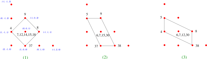
Figure 2: The 3 equivalent representations of the toric diagram of the zeroth Hirzebruch surface as a resolution of $\mathchoice{\hbox{\cmss Z\kern-3.99994ptZ}}{\hbox{\cmss Z\kern-3.99994ptZ}}{\lower 0.9pt\hbox{\cmsss Z\kern-2.79996ptZ}}{\lower 1.2pt\hbox{\cmsss Z\kern-2.79996ptZ}}_{3}\times\mathchoice{\hbox{\cmss Z\kern-3.99994ptZ}}{\hbox{\cmss Z\kern-3.99994ptZ}}{\lower 0.9pt\hbox{\cmsss Z\kern-2.79996ptZ}}{\lower 1.2pt\hbox{\cmsss Z\kern-2.79996ptZ}}_{3}$. We see that (2) and (3) are related by a reflection about the $45^{o}$ line (a symmetry inherent in the parent $\mathchoice{\hbox{\cmss Z\kern-3.99994ptZ}}{\hbox{\cmss Z\kern-3.99994ptZ}}{\lower 0.9pt\hbox{\cmsss Z\kern-2.79996ptZ}}{\lower 1.2pt\hbox{\cmsss Z\kern-2.79996ptZ}}_{3}\times\mathchoice{\hbox{\cmss Z\kern-3.99994ptZ}}{\hbox{\cmss Z\kern-3.99994ptZ}}{\lower 0.9pt\hbox{\cmsss Z\kern-2.79996ptZ}}{\lower 1.2pt\hbox{\cmsss Z\kern-2.79996ptZ}}_{3}$ theory) and we have the two giving equivalent gauge theories as expected.

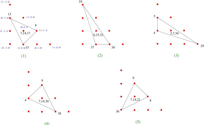
Figure 3: The 5 equivalent representations of the toric diagram of the zeroth del Pezzo surface as a resolution of $\mathchoice{\hbox{\cmss Z\kern-3.99994ptZ}}{\hbox{\cmss Z\kern-3.99994ptZ}}{\lower 0.9pt\hbox{\cmsss Z\kern-2.79996ptZ}}{\lower 1.2pt\hbox{\cmsss Z\kern-2.79996ptZ}}_{3}\times\mathchoice{\hbox{\cmss Z\kern-3.99994ptZ}}{\hbox{\cmss Z\kern-3.99994ptZ}}{\lower 0.9pt\hbox{\cmsss Z\kern-2.79996ptZ}}{\lower 1.2pt\hbox{\cmsss Z\kern-2.79996ptZ}}_{3}$. Again (1) and (4) (respectively (2) and (3)) are related by the $45^{o}$ reflection, and hence give equivalent theories. In fact further analysis shows that all 5 are equivalent.

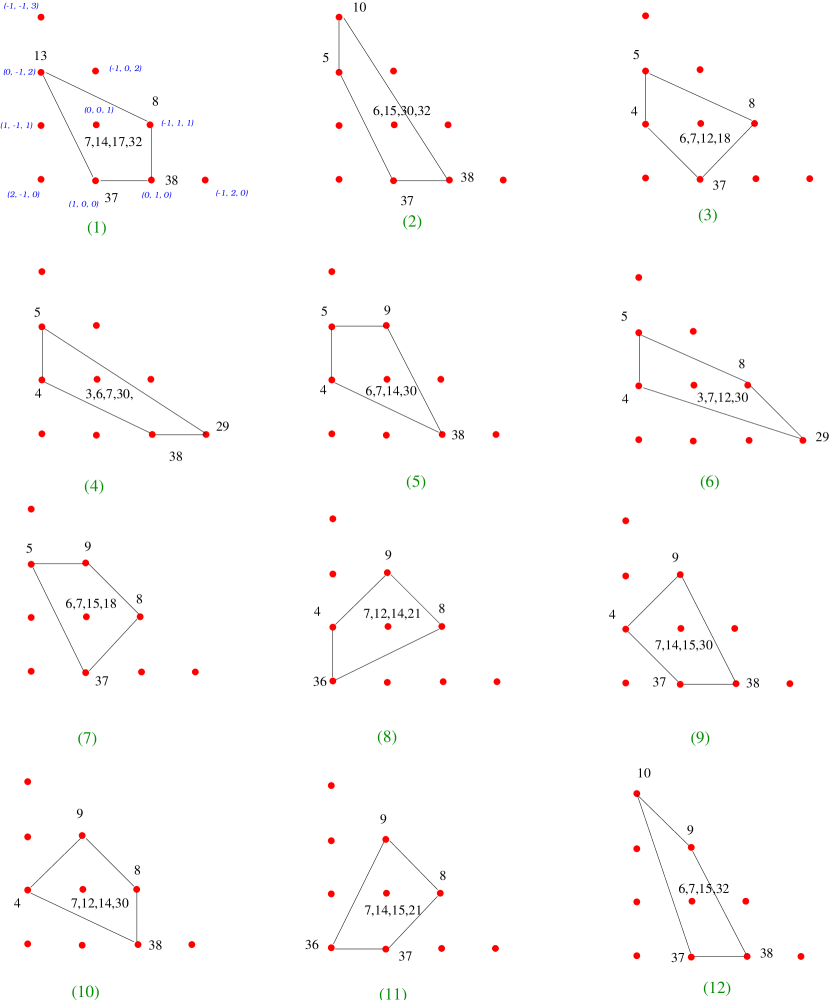
Figure 4: The 12 equivalent representations of the toric diagram of the first del Pezzo surface as a resolution of $\mathchoice{\hbox{\cmss Z\kern-3.99994ptZ}}{\hbox{\cmss Z\kern-3.99994ptZ}}{\lower 0.9pt\hbox{\cmsss Z\kern-2.79996ptZ}}{\lower 1.2pt\hbox{\cmsss Z\kern-2.79996ptZ}}_{3}\times\mathchoice{\hbox{\cmss Z\kern-3.99994ptZ}}{\hbox{\cmss Z\kern-3.99994ptZ}}{\lower 0.9pt\hbox{\cmsss Z\kern-2.79996ptZ}}{\lower 1.2pt\hbox{\cmsss Z\kern-2.79996ptZ}}_{3}$. The pairs (1,5); (2,4); (3,9); (6,12); (7,10) and (8,11) are each reflected by the $45^{o}$ line and give mutually equivalent gauge theories indeed. Further analysis shows that all 12 are equivalent.

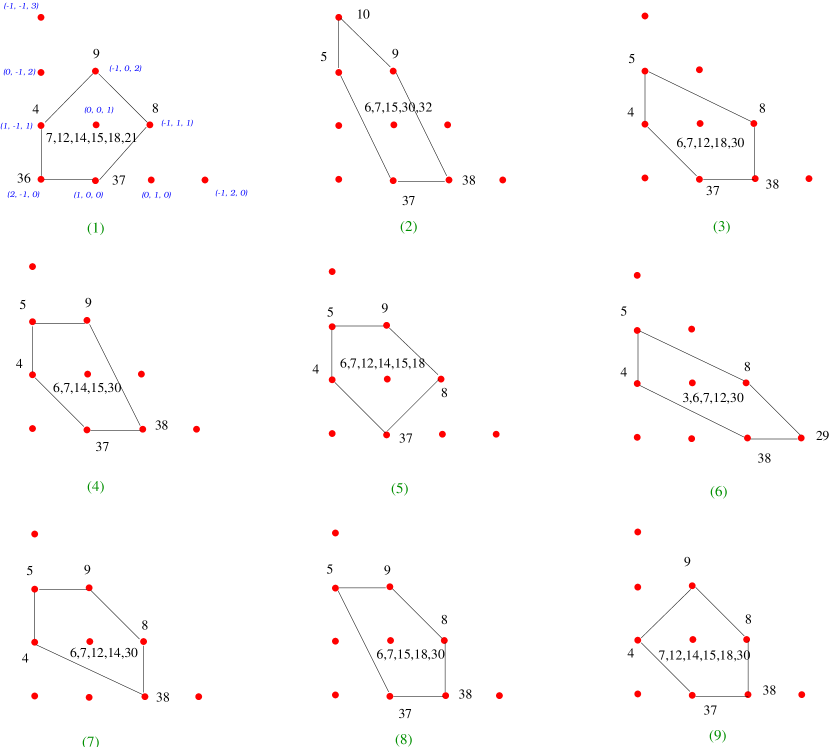
Figure 5: The 9 equivalent representations of the toric diagram of the second del Pezzo surface as a resolution of $\mathchoice{\hbox{\cmss Z\kern-3.99994ptZ}}{\hbox{\cmss Z\kern-3.99994ptZ}}{\lower 0.9pt\hbox{\cmsss Z\kern-2.79996ptZ}}{\lower 1.2pt\hbox{\cmsss Z\kern-2.79996ptZ}}_{3}\times\mathchoice{\hbox{\cmss Z\kern-3.99994ptZ}}{\hbox{\cmss Z\kern-3.99994ptZ}}{\lower 0.9pt\hbox{\cmsss Z\kern-2.79996ptZ}}{\lower 1.2pt\hbox{\cmsss Z\kern-2.79996ptZ}}_{3}$. The pairs (2,6); (3,4); (5,9) and (7,8) are related by $45^{o}$ reflection while (1) is self-reflexive and are hence give pairwise equivalent theories. Further analysis shows that there are two phases given respectively by (1,5,9) and (2,3,4,6,7,8).

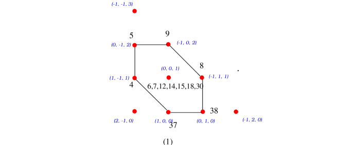
Figure 6: The unique representations of the toric diagram of the third del Pezzo surface as a resolution of $\mathchoice{\hbox{\cmss Z\kern-3.99994ptZ}}{\hbox{\cmss Z\kern-3.99994ptZ}}{\lower 0.9pt\hbox{\cmsss Z\kern-2.79996ptZ}}{\lower 1.2pt\hbox{\cmsss Z\kern-2.79996ptZ}}_{3}\times\mathchoice{\hbox{\cmss Z\kern-3.99994ptZ}}{\hbox{\cmss Z\kern-3.99994ptZ}}{\lower 0.9pt\hbox{\cmsss Z\kern-2.79996ptZ}}{\lower 1.2pt\hbox{\cmsss Z\kern-2.79996ptZ}}_{3}$.

Subsequently, we arrive at a number of D-brane gauge theories; among them, all five cases for $dP^{0}$ are equivalent (which is in complete consistency with the fact that $dP^{0}$ is simply $\hbox{$\,\vrule height=6.45831pt,width=0.4pt,depth=0.0pt\kern-3.00003pt{\rm C}$}^{3}/\mathchoice{\hbox{\cmss Z\kern-3.99994ptZ}}{\hbox{\cmss Z\kern-3.99994ptZ}}{\lower 0.9pt\hbox{\cmsss Z\kern-2.79996ptZ}}{\lower 1.2pt\hbox{\cmsss Z\kern-2.79996ptZ}}_{3}$ and there is only one nontrivial theory for this orbifold, corresponding to the decomposition ${\bf 3}\rightarrow 1+1+1$). For $dP_{1}$, all twelve cases give back to same gauge theory (q.v. Figure 5 of [14]). For $F_{0}$, the three cases give two inequivalent gauge theories as given in §2. Finally for $dP_{2}$, the nine cases again give two different theories. For reference we tabulate the D-term matrix $d$ and F-term matrix $K^{T}$ below. If more than 1 theory are equivalent, then we select one representative from the list, the matrices for the rest are given by transformations (4.3) and (4.8).

$$\begin{array}[]{|c|c|c|}\hline\cr\mbox{Singularity}&\mbox{Matter Content }d&\mbox{Superpotential}\\ \hline\cr(F_{0})_{1}&{\tiny\begin{array}[]{c|cccccccccccc}&X_{1}&X_{2}&X_{3}&X_{4}&X_{5}&X_{6}&X_{7}&X_{8}&X_{9}&X_{10}&X_{11}&X_{12}\\ \hline\cr A&-1&0&-1&0&-1&0&1&1&-1&0&1&1\\ B&0&-1&0&-1&1&0&0&0&1&0&0&0\\ C&0&1&0&1&0&1&-1&-1&0&1&-1&-1\\ D&1&0&1&0&0&-1&0&0&0&-1&0&0\end{array}}&{\footnotesize\begin{array}[]{r}X_{1}X_{8}X_{10}-X_{3}X_{7}X_{10}-X_{2}X_{8}X_{9}-X_{1}X_{6}X_{12}+\\ X_{3}X_{6}X_{11}+X_{4}X_{7}X_{9}+X_{2}X_{5}X_{12}-X_{4}X_{5}X_{11}\end{array}}\\ \hline\cr(F_{0})_{2,3}&{\tiny\begin{array}[]{c|cccccccc}&X_{112}&Y_{122}&Y_{222}&Y_{111}&Y_{211}&X_{121}&X_{212}&X_{221}\\ \hline\cr A&-1&0&0&1&1&0&-1&0\\ B&1&-1&-1&0&0&0&1&0\\ C&0&0&0&-1&-1&1&0&1\\ D&0&1&1&0&0&-1&0&-1\end{array}}&{\tiny\epsilon^{ij}\epsilon^{kl}X_{i~{}12}Y_{k~{}22}X_{j~{}21}Y_{l~{}11}}\\ \hline\cr\hline\cr(dP_{0})_{1,2,3,4,5}&{\tiny\begin{array}[]{c|ccccccccc}&X_{1}&X_{2}&X_{3}&X_{4}&X_{5}&X_{6}&X_{7}&X_{8}&X_{9}\\ \hline\cr A&-1&0&-1&0&-1&0&1&1&1\cr B&0&1&0&1&0&1&-1&-1&-1\cr C&1&-1&1&-1&1&-1&0&0&0\end{array}}&{\footnotesize\begin{array}[]{r}X_{1}X_{4}X_{9}-X_{4}X_{5}X_{7}-X_{2}X_{3}X_{9}-\\ X_{1}X_{6}X_{8}+X_{2}X_{5}X_{8}+X_{3}X_{6}X_{7}\end{array}}\\ \hline\cr\hline\cr(dP_{1})_{1,2,...,12}&{\tiny\begin{array}[]{c|cccccccccc}&X_{1}&X_{2}&X_{3}&X_{4}&X_{5}&X_{6}&X_{7}&X_{8}&X_{9}&X_{10}\\ \hline\cr A&-1&0&0&-1&0&0&0&1&0&1\cr B&1&-1&0&0&0&-1&0&0&1&0\cr C&0&0&1&0&1&0&1&-1&-1&-1\cr D&0&1&-1&1&-1&1&-1&0&0&0\end{array}}&{\footnotesize\begin{array}[]{r}X_{2}X_{7}X_{9}-X_{3}X_{6}X_{9}-X_{4}X_{8}X_{7}-X_{1}X_{2}X_{5}X_{10}\\ +X_{3}X_{4}X_{10}+X_{1}X_{5}X_{6}X_{8}\end{array}}\\ \hline\cr\hline\cr(dP_{2})_{1,5,9}&{\tiny\begin{array}[]{c|ccccccccccccc}&X_{1}&X_{2}&X_{3}&X_{4}&X_{5}&X_{6}&X_{7}&X_{8}&X_{9}&X_{10}&X_{11}&X_{12}&X_{13}\\ \hline\cr A&-1&0&0&-1&0&-1&0&1&0&0&0&1&1\cr B&0&0&-1&0&-1&1&0&0&0&1&0&0&0\cr C&0&0&1&0&1&0&1&-1&-1&0&1&-1&-1\cr D&1&-1&0&0&0&0&0&0&1&-1&0&0&0\cr E&0&1&0&1&0&0&-1&0&0&0&-1&0&0\end{array}}&{\footnotesize\begin{array}[]{r}X_{2}X_{9}X_{11}-X_{9}X_{3}X_{10}-X_{4}X_{8}X_{11}-X_{1}X_{2}X_{7}X_{13}+X_{13}X_{3}X_{6}\\ -X_{5}X_{12}X_{6}+X_{1}X_{5}X_{8}X_{10}+X_{4}X_{7}X_{12}\end{array}}\\ \hline\cr(dP_{2})_{2,3,4,6,7,8}&{\tiny\begin{array}[]{c|cccccccccccc}&X_{1}&X_{2}&X_{3}&X_{4}&X_{5}&X_{6}&X_{7}&X_{8}&X_{9}&X_{10}&X_{11}\\ \hline\cr A&-1&0&-1&0&0&0&1&0&0&0&1\cr B&1&-1&0&0&-1&0&0&0&1&0&0\cr C&0&0&1&-1&0&1&0&0&-1&0&0\cr D&0&0&0&0&0&-1&-1&1&0&1&0\cr E&0&1&0&1&1&0&0&-1&0&-1&-1\end{array}}&{\footnotesize\begin{array}[]{r}X_{5}X_{8}X_{6}X_{9}+X_{1}X_{2}X_{10}X_{7}+X_{11}X_{3}X_{4}\\ -X_{4}X_{10}X_{6}-X_{2}X_{8}X_{7}X_{3}X_{9}-X_{11}X_{1}X_{5}\end{array}}\\ \hline\cr\hline\cr(dP_{3})_{1}&{\tiny\begin{array}[]{c|cccccccccccccc}&X_{1}&X_{2}&X_{3}&X_{4}&X_{5}&X_{6}&X_{7}&X_{8}&X_{9}&X_{10}&X_{11}&X_{12}&X_{13}&X_{14}\\ \hline\cr A&-1&0&0&0&1&0&0&1&-1&0&0&1&-1&0\cr B&0&0&-1&1&0&-1&0&0&0&0&0&0&1&0\cr C&1&-1&0&-1&0&0&0&0&0&0&0&0&0&1\cr D&0&0&1&0&0&0&0&-1&0&-1&1&0&0&0\cr E&0&0&0&0&-1&1&1&0&0&1&0&-1&0&-1\cr F&0&1&0&0&0&0&-1&0&1&0&-1&0&0&0\end{array}}&{\footnotesize\begin{array}[]{r}X_{3}X_{8}X_{13}-X_{8}X_{9}X_{11}-X_{5}X_{6}X_{13}-X_{1}X_{3}X_{4}X_{10}X_{12}\\ +X_{7}X_{9}X_{12}+X_{1}X_{2}X_{5}X_{10}X_{11}+X_{4}X_{6}X_{14}-X_{2}X_{7}X_{14}\end{array}}\\ \hline\cr\end{array}$$

The matter content for these above theories are represented as quiver diagrams in Figure 7 (multi-valence arrows are labelled with a number) and the superpotentials, in the table below.

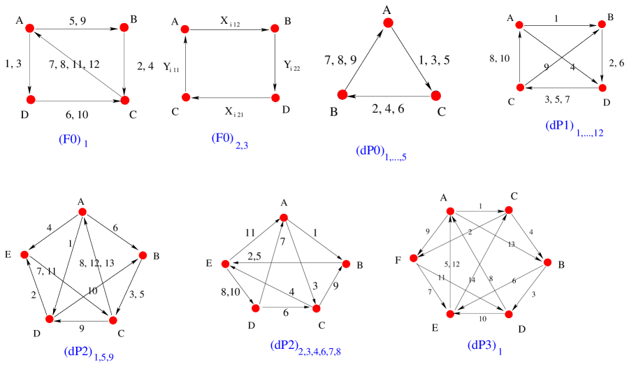
Figure 7: The quiver diagrams for the various phases of the gauge theory for the del Pezzo surfaces and the zeroth Hirzebruch surface.

In all of the above discussions, we have restricted ourselves to the cases of $U(1)$ gauge groups, i.e., with only a single brane probe; this is because such is the only case to which the toric technique can be applied. However, after we obtain the matter contents and superpotential for $U(1)$ gauge groups, we should have some idea for multi-brane probes. One obvious generalization is to replace the $U(1)$ with $SU(N)$ gauge groups directly. For the matter content, the generalization is not so easy. A field with charge $(1,-1)$ under gauge groups $U(1)_{A}\times U(1)_{B}$ and zero for others generalised to a bifundamental $(N,\bar{N})$ of $SU(N)_{A}\times SU(N)_{B}$. However, for higher charges, e.g., charge 2, we simply do not know what should be the generalization in the multi-brane case (for a discussion on generalised quivers cf. e.g. [21]). Furthermore, a field with zero charge under all $U(1)$ groups, generalises to an adjoint of one $SU(N)$ gauge group in the multi-brane case, though we do not know which one.

The generalization of the superpotential is also not so straight-forward. For example, there is a quartic term in the conifold with nonabelian gauge group [17, 18], but it disappears when we go to the $U(1)$ case. The same phenomenon can happen when treating the generic toric singularity.

For the examples we give in this paper however, we do not see any obvious obstruction in the matter contents and superpotential; they seem to be special enough to be trivially generalized to the multi-brane case; they are all charge $\pm 1$ under no more than 2 groups. We simply replace $U(1)$ with $SU(N)$ and $(1,-1)$ fields with bifundamentals while keeping the superpotential invariant. Generalisations to multi-brane stack have also been discussed in [13].

6 Discussions and Prospects

It is well-known that in the study of the world-volume gauge theory living on a D-brane probing an orbifold singularity $\hbox{$\,\vrule height=6.45831pt,width=0.4pt,depth=0.0pt\kern-3.00003pt{\rm C}$}^{3}/\Gamma$, different choices of decomposition into irreducibles of the space-time action of $\Gamma$ lead to different matter content and interaction in the gauge theory and henceforth different moduli spaces (as different algebraic varieties). This strong relation between the decomposition and algebraic variety has been shown explicitly for Abelian orbifolds in [25]. It seems that there is only one gauge theory for each given singularity.

A chief motivation and purpose of this paper is the realisation that the above strong statement can not be generalised to arbitrary (non-orbifold) singularities and in particular toric singularities. It is possible that there are several gauge theories on the D-brane probing the same singularity. The moduli space of these inequivalent theories are indeed by construction the same, as dictated by the geometry of the singularity.

In analogy to the freedom of decomposition into irreps of the group action in the orbifold case, there too exists a freedom in toric singularities: any toric diagram is defined only up to a unimodular transformation (Theorem 3.1). We harness this toric isomorphism as a tool to create inequivalent gauge theories which live on the D-brane probe and which, by construction, flow to the same (toric) moduli space in the IR.

Indeed, these theories constitute another sub-class of examples of toric duality as proposed in [14]. A key point to note is that unlike the general case of the duality (such as F-D ambiguities and repetition ambiguities as discussed therein) of which we have hitherto little control, these particular theories are all physical (i.e., guaranteed to be world-volume theories) by virtue of their being obtainable from the canonical method of partial resolution of Abelian orbifolds. We therefore refer to them as phases of partial resolution.

As a further tool, we have re-examined the Forward and Inverse Algorithms developed in [13, 14, 8] of extracting the gauge theory data and toric moduli space data from each other. In particular we have taken the pains to show what degree of freedom can one have at each step of the Algorithm. This will serve to discriminate whether or not two theories are physically equivalent given their respective matrices at each step.

Thus equipped, we have re-studied the partial resolutions of the Abelian orbifold $\hbox{$\,\vrule height=6.45831pt,width=0.4pt,depth=0.0pt\kern-3.00003pt{\rm C}$}^{3}/(\mathchoice{\hbox{\cmss Z\kern-3.99994ptZ}}{\hbox{\cmss Z\kern-3.99994ptZ}}{\lower 0.9pt\hbox{\cmsss Z\kern-2.79996ptZ}}{\lower 1.2pt\hbox{\cmsss Z\kern-2.79996ptZ}}_{3}\times\mathchoice{\hbox{\cmss Z\kern-3.99994ptZ}}{\hbox{\cmss Z\kern-3.99994ptZ}}{\lower 0.9pt\hbox{\cmsss Z\kern-2.79996ptZ}}{\lower 1.2pt\hbox{\cmsss Z\kern-2.79996ptZ}}_{3})$, namely the 4 toric del Pezzo surfaces $dP_{0,1,2,3}$ and the zeroth Hirzebruch surface $F_{0}$. We performed all possible $SL(3;\mathchoice{\hbox{\cmss Z\kern-3.99994ptZ}}{\hbox{\cmss Z\kern-3.99994ptZ}}{\lower 0.9pt\hbox{\cmsss Z\kern-2.79996ptZ}}{\lower 1.2pt\hbox{\cmsss Z\kern-2.79996ptZ}})$ transformation of these toric diagrams which are up to permutation still embeddable in $\mathchoice{\hbox{\cmss Z\kern-3.99994ptZ}}{\hbox{\cmss Z\kern-3.99994ptZ}}{\lower 0.9pt\hbox{\cmsss Z\kern-2.79996ptZ}}{\lower 1.2pt\hbox{\cmsss Z\kern-2.79996ptZ}}_{3}\times\mathchoice{\hbox{\cmss Z\kern-3.99994ptZ}}{\hbox{\cmss Z\kern-3.99994ptZ}}{\lower 0.9pt\hbox{\cmsss Z\kern-2.79996ptZ}}{\lower 1.2pt\hbox{\cmsss Z\kern-2.79996ptZ}}_{3}$ and subsequently initiated the Inverse Algorithm therewith. We found at the end of the day, in addition to the physical theories for these examples presented in [14], an additional one for both $F_{0}$ and $dP_{2}$. Further embedding can of course be done, viz., into $\mathchoice{\hbox{\cmss Z\kern-3.99994ptZ}}{\hbox{\cmss Z\kern-3.99994ptZ}}{\lower 0.9pt\hbox{\cmsss Z\kern-2.79996ptZ}}{\lower 1.2pt\hbox{\cmsss Z\kern-2.79996ptZ}}_{n}\times\mathchoice{\hbox{\cmss Z\kern-3.99994ptZ}}{\hbox{\cmss Z\kern-3.99994ptZ}}{\lower 0.9pt\hbox{\cmsss Z\kern-2.79996ptZ}}{\lower 1.2pt\hbox{\cmsss Z\kern-2.79996ptZ}}_{n}$ for $n>3$; it is expected that more phases would arise for these computationally prohibitive cases, for example for $dP_{3}$.

A clear goal awaits us: because for the generic (non-orbifold) toric singularity there is no concrete concept corresponding to the different decomposition of group action, we do not know at this moment how to classify the phases of toric duality. We certainly wish, given a toric singularity, to know (a) how many inequivalent gauge theory are there and (b) what are the corresponding matter contents and superpotential. It will be a very interesting direction for further investigation.

Many related questions also arise. For example, by the AdS/CFT correspondence, we need to understand how to describe these different gauge theories on the supergravity side while the underline geometry is same. Furthermore the $dP^{2}$ theory can be described in the brane setup by $(p,q)$-5 brane webs [24], so we want to ask how to understand these different phases in such brane setups. Understanding these will help us to get the gauge theory in higher del Pezzo surface singularities.

Another very pertinent issue is to clarify the meaning of “toric duality.” So far it is merely an equivalence of moduli spaces of gauge theories in the IR. It would be very nice if we could make this statement stronger. For example, could we find the explicit mappings between gauge invariant operators of various toric-dual theories? Indeed, we believe that the study of toric duality and its phase structure is worth further pursuit.

7 Appendix: Gauge Theory Data for $\mathchoice{\hbox{\cmss Z\kern-3.99994ptZ}}{\hbox{\cmss Z\kern-3.99994ptZ}}{\lower 0.9pt\hbox{\cmsss Z\kern-2.79996ptZ}}{\lower 1.2pt\hbox{\cmsss Z\kern-2.79996ptZ}}_{n}\times\mathchoice{\hbox{\cmss Z\kern-3.99994ptZ}}{\hbox{\cmss Z\kern-3.99994ptZ}}{\lower 0.9pt\hbox{\cmsss Z\kern-2.79996ptZ}}{\lower 1.2pt\hbox{\cmsss Z\kern-2.79996ptZ}}_{n}$

For future reference we include here the gauge theory data for the $\mathchoice{\hbox{\cmss Z\kern-3.99994ptZ}}{\hbox{\cmss Z\kern-3.99994ptZ}}{\lower 0.9pt\hbox{\cmsss Z\kern-2.79996ptZ}}{\lower 1.2pt\hbox{\cmsss Z\kern-2.79996ptZ}}_{n}\times\mathchoice{\hbox{\cmss Z\kern-3.99994ptZ}}{\hbox{\cmss Z\kern-3.99994ptZ}}{\lower 0.9pt\hbox{\cmsss Z\kern-2.79996ptZ}}{\lower 1.2pt\hbox{\cmsss Z\kern-2.79996ptZ}}_{n}$ orbifold, so that, as mentioned in [14], any 3-dimensional toric singularity may exist as a partial resolution thereof.

We have $3n^{2}$ fields denoted as $X_{ij},Y_{ij},Z_{ij}$ and choose the decomposition ${\bf 3}\rightarrow(1,0)+(0,1)+(-1,-1)$. The matter content (and thus the $d$ matrix) is well-known from standard brane box constructions, hence we here focus on the superpotential [23] (and thus the $K$ matrix):

$$X_{ij}Y_{i(j+1)}Z_{(i+1)(j+1)}-Y_{ij}X_{(i+1)j}Z_{(i+1)(j+1)},$$

from which the F-terms are

$$\begin{array}[]{crcl}\frac{\partial W}{\partial X_{ij}}:&Y_{i(j+1)}Z_{(i+1)(j+1)}&=&Z_{i(j+1)}Y_{(i-1)j}\\ &&&\\ \frac{\partial W}{\partial Y_{ij}}:&Z_{(i+1)j}X_{i(j-1)}&=&X_{(i+1)j}Z_{(i+1)(j+1)}\\ &&&\\ \frac{\partial W}{\partial Z_{(i+1)(j+1)}}:&X_{ij}Y_{i(j+1)}&=&Y_{ij}X_{(i+1)j}.\end{array}$$ (7.20)

Now let us solve (7.20). First we have $Y_{i(j+1)}=Y_{ij}X_{(i+1)j}/X_{ij}$. Thus if we take $Y_{i0}$ and $X_{ij}$ as the independent variables, we have

$$Y_{i(j+1)}=\frac{\prod_{l=0}^{j}X_{(i+1)l}}{\prod_{l=0}^{j}X_{il}}Y_{i0}.$$ (7.21)

There is of course the periodicity which gives

$$Y_{in}=Y_{i0}\Longrightarrow\prod_{l=0}^{n-1}X_{(i+1)l}=\prod_{l=0}^{n-1}X_{il}.$$ (7.22)

Next we use $X_{ij}$ to solve the $Z_{ij}$ as $Z_{i(j+1)}=Z_{ij}X_{(i-1)(j-1)}/X_{ij},$ whence

$$Z_{i(j+1)}=\frac{\prod_{l=0}^{j}X_{(i-1)(l-1)}}{\prod_{l=0}^{j}X_{il}}Z_{i0}.$$ (7.23)

As above,

$$Z_{in}=Z_{i0}\Longrightarrow\prod_{l=0}^{n-1}X_{(i-1)(l-1)}=\prod_{l=0}^{n-1}X_{il}.$$ (7.24)

Putting the solution of $Y,Z$ into the first equation of (7.20) we get

$$\frac{\prod_{l=0}^{j}X_{(i+1)l}}{\prod_{l=0}^{j}X_{il}}Y_{i0}\frac{\prod_{l=0}^{j}X_{(i)(l-1)}}{\prod_{l=0}^{j}X_{(i+1)l}}Z_{(i+1)0}=\frac{\prod_{l=0}^{j}X_{(i-1)(l-1)}}{\prod_{l=0}^{j}X_{il}}Z_{i0}\frac{\prod_{l=0}^{j-1}X_{il}}{\prod_{l=0}^{j-1}X_{(i-1)l}}Y_{(i-1)0},$$

which can be simplified as $Y_{i0}Z_{(i+1)0}X_{i(n-1)}=Z_{i0}Y_{(i-1)0}X_{(i-1)(n-1)}$, or $X_{i(n-1)}=X_{(i-1)(n-1)}\frac{Y_{(i-1)0}}{Y_{i0}}\frac{Z_{i0}}{Z_{(i+1)0}}$. From this we solve

$$X_{i(n-1)}=X_{0(n-1)}\prod_{l=0}^{i-1}\frac{Y_{l0}}{Y_{(l+1)0}}\frac{Z_{(l+1)0}}{Z_{(l+2)0}}.$$ (7.25)

The periodicity gives

$$\prod_{l=0}^{n-1}\frac{Y_{l0}}{Y_{(l+1)0}}\frac{Z_{(l+1)0}}{Z_{(l+2)0}}=1.$$ (7.26)

Now we have the independent variables $Y_{i0}$ $Z_{i0}$ and $X_{ij}$ for $j\neq n-1$ and $X_{0(n-1)}$, plus three constraints (7.22) (7.24) (7.26). In fact, considering the periodic condition for $X$, (7.22) is equivalent to (7.24). Furthermore considering the periodic conditions for $Z_{i0}$ and $Y_{i0}$, (7.26) is trivial. So we have only one constraint. Putting the expression (7.25) into (7.22) we get $\prod_{l=0}^{n-2}X_{(i+1)l}\frac{Y_{i0}}{Y_{(i+1)0}}\frac{Z_{(i+1)0}}{Z_{(i+2)0}}=\prod_{l=0}^{n-2}X_{il}\Rightarrow\prod_{l=0}^{n-2}X_{(i+1)l}\frac{1}{Y_{(i+1)0}Z_{(i+2)0}}=\prod_{l=0}^{n-2}X_{il}\frac{1}{Y_{i0}Z_{(i+1)0}}.$

From this we can solve the $X_{i(n-1)}$ for $i\neq 0$ as

$$X_{i(n-2)}=(\prod_{l=0}^{n-2}X_{0l})\frac{Y_{i0}Z_{(i+1)0}}{Y_{00}Z_{10}}(\prod_{l=0}^{n-2}X_{il})^{-1}.$$ (7.27)

The periodic condition does not give new constraints.

Now we have finished solving the F-term and can summarise the results into the $K$-matrix. We use the following independent variables: $Z_{i0}$, $Y_{i0}$ for $i=0,1,...,n-1$; $X_{ij}$ for $i=0,1,...,n-1$ $j=0,1,...,n-3$ and $X_{0(n-2)}$ $X_{0(n-1)}$, so the total number of variables is $2n+n(n-2)+2=n^{2}+2$. This is usually too large to calculate. For example, even when $n=4$, the $K$ matrix is $48\times 18$. The standard method to find the dual cone $T$ from $K$ needs to analyse some $48!/(17!31!)$ vectors, which is computationally prohibitive.

References

• [1] B. Greene, “String Theory on Calabi-Yau Manifolds,” hep-th/9702155.
• [2] E. Witten, “Phases of $N=2$ theories in two dimensions”, hep-th/9301042.
• [3] M. Douglas and G. Moore, “D-Branes, Quivers, and ALE Instantons,” hep-th/9603167.
• [4] Clifford V. Johnson, Robert C. Myers, “Aspects of Type IIB Theory on ALE Spaces,” Phys.Rev. D55 (1997) 6382-6393.hep-th/9610140.
• [5] S. Kachru and E. Silverstein, “4D Conformal Field Theories and Strings on Orbifolds,” hep-th/9802183.
• [6] D. R. Morrison and M. Ronen Plesser, “Non-Spherical Horizons I”, hep-th/9810201.
• [7] A. Lawrence, N. Nekrasov and C. Vafa, “On Conformal Field Theories in Four Dimensions,” hep-th/9803015.
• [8] Michael R. Douglas, Brian R. Greene, and David R. Morrison, “Orbifold Resolution by D-Branes”, hep-th/9704151.
• [9] A. Hanany and E. Witten, “Type IIB Superstrings, BPS monopoles, and Three-Dimensional Gauge Dynamics,” hep-th/9611230.
• [10] A. Hanany and A. Zaffaroni, “On the Realisation of Chiral Four-Dimensional Gauge Theories Using Branes,” hep-th/9801134.
• [11] A. Hanany and A. Uranga, “Brane Boxes and Branes on Singularities,” hep-th/9805139.
• [12] A. Hanany and Y.-H. He, “Non-Abelian Finite Gauge Theories,” hep-th/9811183.
• [13] Chris Beasley, Brian R. Greene, C. I. Lazaroiu, and M. R. Plesser, “D3-branes on partial resolutions of abelian quotient singularities of Calabi-Yau threefolds,” hep-th/9907186.
• [14] Bo Feng, Amihay Hanany and Yang-Hui He, “D-Brane Gauge Theories from Toric Singularities and Toric Duality,” hep-th/0003085.
• [15] Tapobrata Sarkar, “D-brane gauge theories from toric singularities of the form $C^{3}/\Gamma$ and $C^{4}/\Gamma$,” hep-th/0005166.
• [16] Igor R. Klebanov, Edward Witten, “Superconformal Field Theory on Threebranes at a Calabi-Yau Singularity,” hep-th/9807080.
• [17] J. Park, R. Rabadan, A. M. Uranga, “Orientifolding the conifold”, Nucl.Phys. B570 (2000) 38-80, hep-th/9907086.
• [18] Brian R. Greene, “D-Brane Topology Changing Transitions,” Nucl.Phys. B525 (1998) 284-296.
• [19] W. Fulton, “Introduction to Toric Varieties,” Princeton University Press, 1993.
• [20] B. Sturmfels, “Grobner Bases and Convex Polytopes,” Univ. Lecture Series 8. AMS 1996.
• [21] Y.-H. He, “Some Remarks on the Finitude of Quiver Theories,” hep-th/9911114.
• [22] Günter Ewald, “Combinatorial Convexity and Algebraic Geometry,” Springer-Verlag, NY. 1996.
• [23] A. Hanany, M. J. Strassler and A. M. Uranga, “Finite theories and marginal operators on the brane,” JHEP 9806, 011 (1998), hep-th/9803086.
• [24] Ofer Aharony, Amihay Hanany, Barak Kol, “Webs of (p,q) 5-branes, Five Dimensional Field Theories and Grid Diagrams”, Nucl.Phys. B505 (1997) 625-640, hep-th/9703003
• [25] P. Aspinwall, “Resolution of Orbifold Singularities in String Theory,” hep-th/9403123.